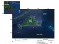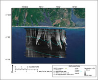
Figure 1. Location map showing the USGS Cruise 07011 survey bounds and the Woods Hole Oceanographic Institute (WHOI) Martha's Vineyard Coastal Observatory (MVCO) locations. Environmental Systems Research Institute (ESRI) USA Prime Imagery is used as background image (I-cubed, 2009). Click on figure for larger image.

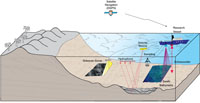Figure 3. Illustration of the geophysical systems used to characterize the seafloor during USGS Cruise 07011. Sidescan-sonar, swath bathymetric, and seismic-reflection systems were used to define the surficial sediment distribution, depth, and underlying geology. Sampling systems were used to collect direct samples of the seafloor sediment. A Differential Global Positioning System (DGPS) was used to navigate the sidescan-sonar and swath bathymetric systems, while a Global Positioning System (GPS) was used to navigate the seismic-reflection system. Click on figure for larger image.

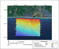Figure 4. Color shaded-relief image of bathymetric data collected by the USGS during Cruise 07011. Depth is in meters and ranges from approximately 6 to 24 meters water depth. No data were collected in the gray regions, where moored instruments and structures were located. The locations of Martha's Vineyard Coastal Observatory (MVCO) (yellow dots) and sound velocity profiles (red dots) collected during USGS Cruise 07011 are also displayed. Environmental Systems Research Institute (ESRI) USA Prime Imagery is used as background image. Click on figure for larger image.

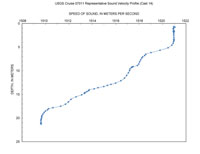Figure 5. Representative sound velocity profile (SVP) displaying the speed of sound in the water column, in meters per second, versus water depth, in meters. These data were collected at SVP location 14 during USGS Cruise 07011. The data reveal the characteristic negative gradient, with presumably warmer surface waters overlying relatively cooler sub-surface waters. Click on figure for larger image.

Figure 6. Sidescan-sonar mosaic collected by the USGS during Cruise 07011. Sidescan-sonar backscatter values (relative strength of return) are displayed as digital numbers (DN), on a relative scale, high-backscatter is represented by light tones within the image and low backscatter is represented by dark tones. The locations of Martha's Vineyard Coastal Observatory (MVCO) (yellow dots) and 5-meter bathymetric contours are also displayed. Environmental Systems Research Institute (ESRI) USA Prime Imagery is used as background image. Click on figure for larger image.

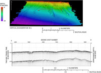Figure 7. TOP: Color-shaded image of swath bathymetric data collected during USGS Cruise 07011. Depth is displayed in meters and ranges from approximately 6 to 24 meters water depth. Vertical exaggeration is 50 times. Sun illumination is from the northeast. Location of seismic-reflection line is displayed. BOTTOM: seismic-reflection data collected during USGS Cruise 07011. See top image for location. Depth is displayed as two-way travel time. Approximate depth is displayed in meters and assumes a speed of sound of 1,500 meters per second. Seismic shot number is displayed across the top of the profile. Several features are visible within the seismic image. At shot 5000, a sub-surface channel is visible within the seismic record, and reflections from shots 7000 to 9000 reveal an unconformity underlying low-relief bedforms. The bedforms are visible within the swath bathymetric image. Click on figure for larger image.

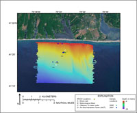Figure 8. Color shaded-relief image of bathymetric data collected by the USGS during Cruise 07011. Depth is in meters and ranges from approximately 6 to 24 meters water depth. No data were collected in the gray regions, where moored instruments and structures were located. The locations of MVCO and beach and seafloor sediment samples collected in 2005 (green dots) and 2007 (blue dots) are also displayed. Environmental Systems Research Institute (ESRI) USA Prime Imagery is used as background image. Click on figure for larger image.

The following sections provide basic descriptions of shipboard acquisition and post-cruise processing of the geophysical and geospatial data contained in this report. Detailed descriptions of acquisition parameters, post-processing steps, and accuracy assessments for each data type are provided within the metadata files for geospatial data layers in the GIS Data Catalog.

Field Program

In August 2007, the USGS WHSC conducted a nearshore geophysical mapping effort off the south coast of Martha's Vineyard in the vicinity of the WHOI MVCO aboard the Megan T. Miller (fig. 1). The study area covers 35 square kilometers (km²) from ~0.2 km to ~5 km offshore and ranges in depth from ~6 to 23 m. The following high-resolution systems were used to map bathymetry (depth), the surficial sediment distribution, and the sub-surface geology: a Systems Engineering and Assessment, Ltd., SWATHplus interferometric (swath) sonar (234 kilohertz (kHz)), a Klein Associates 3000 dual-frequency (100/500 kHz) sidescan sonar, and an EdgeTech 512i chirp subbottom profiler (500 Hz -12 kHz) (fig. 3).

All geophysical systems were run concurrently at shore-parallel line spacing ranging from 40-m spacings in water depths less than 15 m and 70-m line spacing in water depths greater than 15 m. Swath bathymetric and seismic data were also collected along shore-perpendicular lines with a 500-m to 1-km line spacing.

Swath Bathymetry

During USGS Cruise 07011, approximately 660 km of swath bathymetric data were acquired with a SEA Ltd. SWATHplus 234-kHz interferometric bathymetric sonar (Systems Engineering and Assessment, Ltd., 2009) (fig. 4). The SWATHplus transducers and a CodaOctopus F180R Motion Reference Unit (MRU) (CodaOctopus Group, Inc., 2009) were mounted on a rigid vertical pole and positioned on the starboard side of the Megan T. Miller about 2.5 m below the water line. Two Differential Global Positioning System (DGPS) navigation antennas and one Real-Time Kinematic (RTK) navigation antenna were mounted directly above (6.76 m) the transducers and MRU on a rigid horizontal pole as part of the sidemount configuration.

SWATHplus acquisition software was used to acquire the swath bathymetry at a 0.125 second (s) ping rate and digitally log the data at a 2 kilobyte (kB) sample rate. Ship motion (pitch, heave, roll, and heading) and position were acquired with the F180R series MRU and transmitted via network connections to the SWATHplus acquisition software. Fourteen sound velocity profiles (SVP) were collected at various locations throughout the survey area at time intervals ranging from 2 to 12 hours using an Applied Microsystems SV Plus v2 sound velocimeter (Applied Microsystems, 2009). SVP data were incorporated into the SWATHplus acquisition software and used to minimize refraction artifacts due to changes in the sound velocity structure of the water column. SVPs were generally collected at the eastern and western ends of the survey area. This procedure was followed primarily to coordinate collection of SVPs with the beginning or end of tracklines, simplifying SVP data collection and minimizing the need to stop and restart geophysical data collection and maneuver the ship within the middle of the survey area. Ideally, SVPs would be collected continuously throughout the survey area in order to map fine-scale changes in the speed of sound structure of the water column. However, only small variations in the speed of sound and negligible refraction artifacts present in the swath bathymetric data allowed for broad-scale mapping of the speed of sound within the study area. Generally, the shallow-water SVPs displayed a negative gradient, with presumably warmer surface waters, ranging in depth from roughly 2 to 10 m, overlying relatively cooler, deeper waters ranging in depth from roughly 5 to 15 m (fig. 5).

Swath bathymetric data were referenced to a local vertical datum at the WHOI MVCO. MVCO maintains an instrumented node at a depth of 12 m that records a variety of oceanographic data including water level heights above the node (fig. 4). Recorded oscillation of the water level above the node was used to reference the bathymetric data. These data are not tied into any chart datum (that is, Mean Lower Low Water) but, rather, represent a long-term mean water depth directly above the MVCO node (11.68 m, August 2006 - present). This local vertical reference system was chosen as the vertical datum because several datasets, all relative to the MVCO node, will be utilized in oceanographic modeling.

SWATHplus, Computer Aided Resource Information System (CARIS, 2009), and Interactive Visualization Systems (IVS, 2009) processing software packages were used to post-process the swath bathymetric data. Navigation data were edited to remove outliers (that is, poor-quality navigation positions), and raw bathymetric soundings were filtered to remove spurious soundings, rectified for ship motion and changes in the speed of sound within the water column, and referenced to the local vertical datum (MVCO) within SWATHplus. CARIS software was used to grid the processed data at a 2-m cell size by averaging the high-density data and to apply a 5x5 grid cell median filter to the composite grid. The tight line spacing during data acquisition provided complete seafloor coverage, thus limiting the need for interpolation within the gridded data to infill data gaps between survey tracklines. Data gaps exist where the ship had to steer around obstacles, such as the components of the MVCO. IVS software (IVS, 2009) was used to generate Digital Terrain Models (DTM) and export Environmental Systems Research Institute (ESRI) format ASCII raster grids for inclusion in a GIS. All gridded data are projected in Universal Transverse Mercator (UTM), Zone 19 N, meters, referenced to WGS84 horizontal datum.

Sidescan Sonar

Approximately 620 km of shore-parallel sidescan-sonar data were acquired with a Klein System 3000 digital sidescan-sonar (Klein Associates, Inc., 2009) (fig. 6). This dual-frequency sonar acquires data at nominal frequencies of 100 and 500 kHz (actually 132 and 445 kHz). The 100-kHz data were used to generate the composite sidescan-sonar mosaic (fig. 6).

The sidescan sonar was towed from the starboard side of the Megan T. Miller. A DGPS antenna positioned on the starboard aft roof of the USGS mobile acquisition lab was used to acquire positions. A digital cable-out display was used to measure towfish layback. Layback and DGPS input, and their relative offsets, were used by the Klein SonarPro acquisition software to calculate position of the sonar towfish. SonarPro acquired raw data files in eXtended Triton Format (XTF) format at a 0.03-s ping rate yielding a 50-m range (100-m swath).

XSonar/Showimage sonar processing software packages were used to correct for geometric and radiometric distortions inherent in the sonar data (Danforth, 1991; 1997). PCI Geomatica software (Geomatica, 2009) was used to generate georeferenced sidescan-sonar mosaics for the 100-kHz sidescan-sonar data (Paskevich, 1996). Gray-scale TIFF images were produced at a 0.5-m resolution and referenced to the World Geodetic System of 1984 (WGS84), Universal Transverse Mercator (UTM-Zone 19) Coordinate System. A linear stretch was applied to the TIFF image to increase the dynamic range of the data. TIFF images were incorporated into a GIS. Environmental Systems Research Institute (ESRI) world files (*tfw) are associated with each TIFF image and define the upper left coordinates and image resolution.

Chirp Seismic Reflection

Approximately 680 km of seismic-reflection data were collected using an EdgeTech Geo-Star full spectrum sub-bottom (FSSB) system and a SB-0512i towfish with a swept frequency range of 0.5 – 12 kHz (EdgeTech, 2009) (fig. 7). The 512i towfish was mounted on a catamaran and towed approximately 5 m off the stern of the Megan T. Miller and 1.5 m below the sea surface. A GPS navigation receiver was mounted on the seismic catamaran to provide towfish navigation. GPS positions were transmitted to a receiver positioned on the center, aft of the USGS mobile acquisition van and input to the seismic acquisition software. EdgeTech J-Star seismic acquisition software was used to control the Geo-Star topside unit and digitally log trace data in EdgeTech native format (JSF) (Edgetech, 2009). Data were acquired using a 0.25-s shot rate, 5 millisecond (ms) pulse length, and a 0.5-to 8.0-kHz swept frequency. Recorded trace lengths were approximately 250-ms.

The JSF format trace data were converted to SEG-Y format using an in-house C program, jsf2segy. SIOSEIS (SIOSEIS, 2007) and Seismic Unix (Stockwell and Cohen, 2007) were used to post-process the raw chirp seismic-reflection data. Navigation data were inspected and edited to remove outliers, static corrections were applied to correct for towfish depth beneath the sea surface, seafloor reflections were identified by peak amplitude, and sea-surface heave was removed. Final trace data, plotted as JPEG images, and geo-located shot-point trackline files are presented in this report. JPEG images and seismic navigation are also incorporated within a GIS.

Supplemental Data: Sediment Samples

Included within this data release are onshore beach and seafloor sediment samples collected near the MVCO by investigators participating in the ONR-funded OASIS and Ripples (DRI) projects(fig. 8). Beach and seafloor samples were generally collected to locate the boundary between coarse and fine sediment along low-amplitude rippled bedforms prior to deployment and retrieval of instrumented tripods and to document the physical characteristics of the beach (Sherwood and others, 2009). Samples were not collected to ground-truth the geophysical data acquired during USGS Cruise 07011.

The sample data are contained within the GIS catalog and in a Comma Separated Value (CSV) file. All samples were processed for grain-size analyses in the Woods Hole Science Center's sediment lab using sieve and coulter counter techniques (Poppe and others, 2005). Beach samples (top 2 centimeters (cm)) were hand sampled with a Teflon-coated scoop. The majority of seafloor samples were obtained by SCUBA divers with short (~15 to -30-cm long x -4.5-cm diameter) push cores, but a few samples were collected with a modified Van Veen grab sampler and subsampled to obtain representative material from the top 2 cm. Samples were collected in September 2005 and August and October 2007.