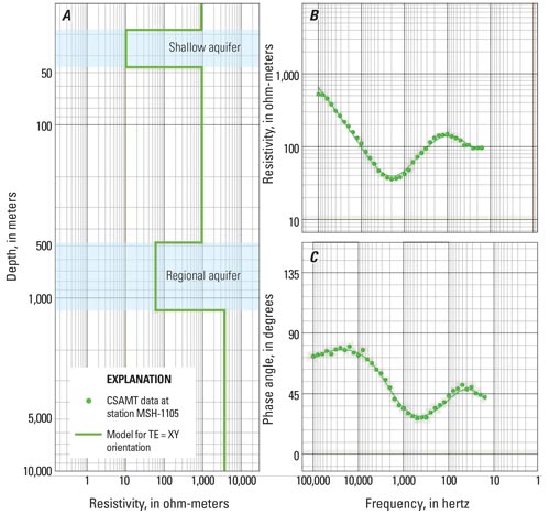
Skip Links

USGS - science for a changing world

Data Series 901


Southerly view into the crater of Mount St. Helens

Mount St. Helens: Controlled-Source Audio-Frequency Magnetotelluric (CSAMT) Data and Inversions


Skip past contents information
Cover
Introduction
Data Acquisition
GPS Data
EDI Data
Data Processing
Occam Inversions
Fischer Inversions
Marquardt Inversions
References
Index page

Marquardt Inversions

A Marquardt inversion is a damped, least-squares ridge-regression algorithm used to obtain conductivity versus depth from electromagnetic sounding data (see fig. 5). It requires a starting model that has equal to or less than the number of layers that can reasonably be observed in a Fischer inversion. The algorithm modifies the resistivities and thicknesses of the specified number of layers until it minimizes the least-squares error between the model response and the observed data. It is very sensitive to the starting (initial) model and commonly will not work if one attempts to invert for more layers than are resolved by the data (Marquardt, 1963; Pujol, 2007).

All Marquardt Inversions were done for the TE = XY orientation. If there was apparent anisotropy, the inversion was also done for TE = YX.

MSH -1002-Marquardt-YX.pdf (= MSH-1001)

MSH -1003-Marquardt-XY.pdf (= MSH-1004)

MSH -1102-Marquardt-XY.pdf

MSH -1103-Marquardt-XY.pdf

MSH -1103-Marquardt-YX.pdf

MSH -1104-Marquardt-XY.pdf

MSH -1105-Marquardt-XY.pdf

MSH -1106-Marquardt-XY.pdf

MSH -1106-Marquardt-YX.pdf

MSH -1107-Marquardt-XY.pdf

MSH -1108-Marquardt-XY.pdf

MSH -1109-Marquardt-XY.pdf

MSH -1109-Marquardt-YX.pdf

MSH -1110-Marquardt-XY.pdf

MSH -1110-Marquardt-YX.pdf

Figure 5. Example of a Marquardt Inversion of the controlled-source audio-frequency magnetotelluric (CSAMT) data. A, The computer inversion of the data into a resistivity versus depth vertical profile for station MSH-1105. In this figure, the separate shallow (glacier-fed) and regional aquifers are shown in light blue. B, The original resistivity data and the inversion model fit for resistivity as a function of measurement frequency. C, The original phase data and the inversion model fit for phase as a function of measurement frequency. The fit shown between data and model in all three frames of this figure was achieved in 10 iterations, with a 0.00165 least-squares error.

Figure 5. Example of a Marquardt Inversion of the controlled-source audio-frequency magnetotelluric (CSAMT) data. A, The computer inversion of the data into a resistivity versus depth vertical profile for station MSH-1105. In this figure, the separate shallow (glacier-fed) and regional aquifers are shown in light blue. B, The original resistivity data and the inversion model fit for resistivity as a function of measurement frequency. C, The original phase data and the inversion model fit for phase as a function of measurement frequency. The fit shown between data and model in all three frames of this figure was achieved in 10 iterations, with a 0.00165 least-squares error.

Accessibility FOIA Privacy Policies and Notices

Take Pride in America logo USA.gov logo U.S. Department of the Interior | U.S. Geological Survey
URL: http://pubsdata.usgs.gov/pubs/ds/0901/marquardt_inversions.html
Page Contact Information: GS Pubs Web Contact
Page Last Modified: Monday, 28-Nov-2016 20:31:49 EST