Image Classification

A hybrid classification approach (fig. 2) was used to minimize misclassification of small interior water bodies and tidal channels with surrounding marsh environments:

1. A 3×3 (pixel) edge enhancement convolution filter was applied to the radiometrically corrected, mosaicked images to enhance small water features;
   
   
2. Unsupervised classification was performed on the edge-enhanced image to identify and extract water areas;
   
   
3. Water areas from (2) were masked from the non edge-enhanced image, and unsupervised classification of the remaining pixels was grouped into seven classes (water, wet marsh, marsh, forested, mixed vegetation, vegetated bare earth, and bare earth);
   
   
4. Results of (2) and (3) were merged to generate a final thematically classified raster dataset; and
   
   
5. Line feature classes representing open-ocean, back-barrier, and estuarine mainland shoreline positions and beach/sand-line positions were generated from (4).

Image classification was performed using Intergraph Corporation ERDAS IMAGINE 2014 software. Thematic raster data were converted to sand- and shoreline feature datasets using Esri ArcGIS version 10.2. ERDAS IMAGINE uses the ISODATA (Iterative Self-Organizing Data Analysis Technique) clustering algorithm to perform unsupervised classification (Intergraph Corporation, 2013). The K-means option with maximum of 25 iterations and 0.95 convergence threshold was used to generate 50 spectral clusters (classes) for each unsupervised analysis in this study. These clusters were subsequently grouped into seven land-cover classes on the basis of visual interpretation of the source imagery: water, wet marsh, marsh, forested, mixed vegetation, vegetated bare earth, and bare earth. False-color RGB (red-green-blue) visual displays using bands 4, 5, 3 and 7, 5, 4 provided the best contrast for discriminating between land-cover classes.

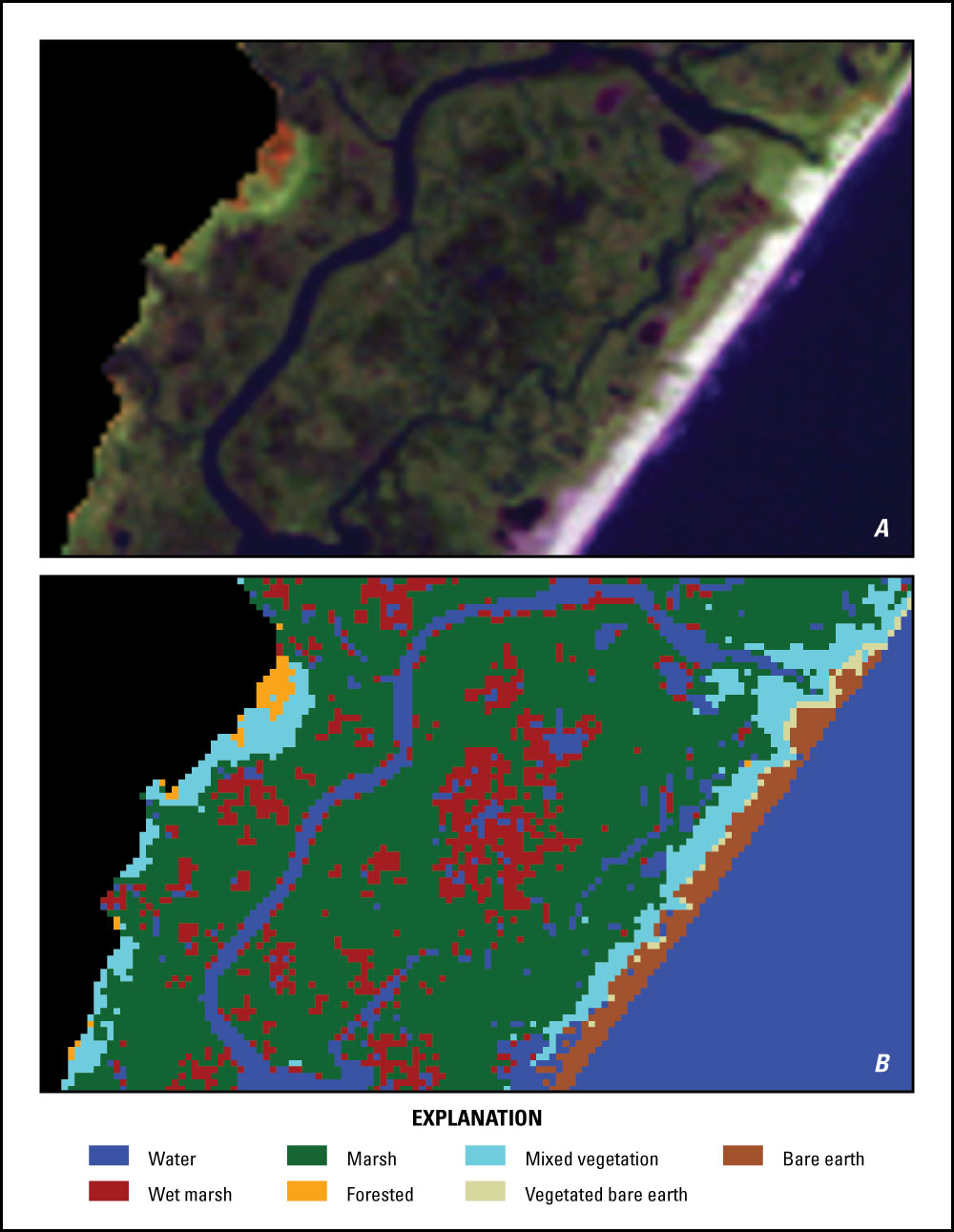
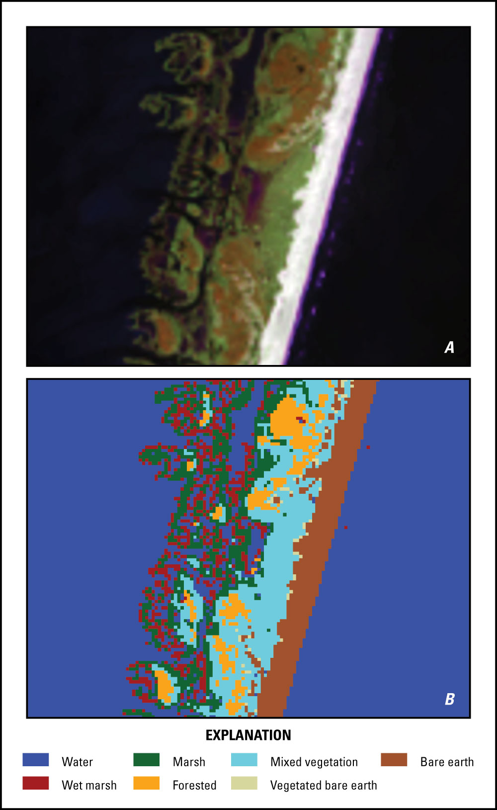
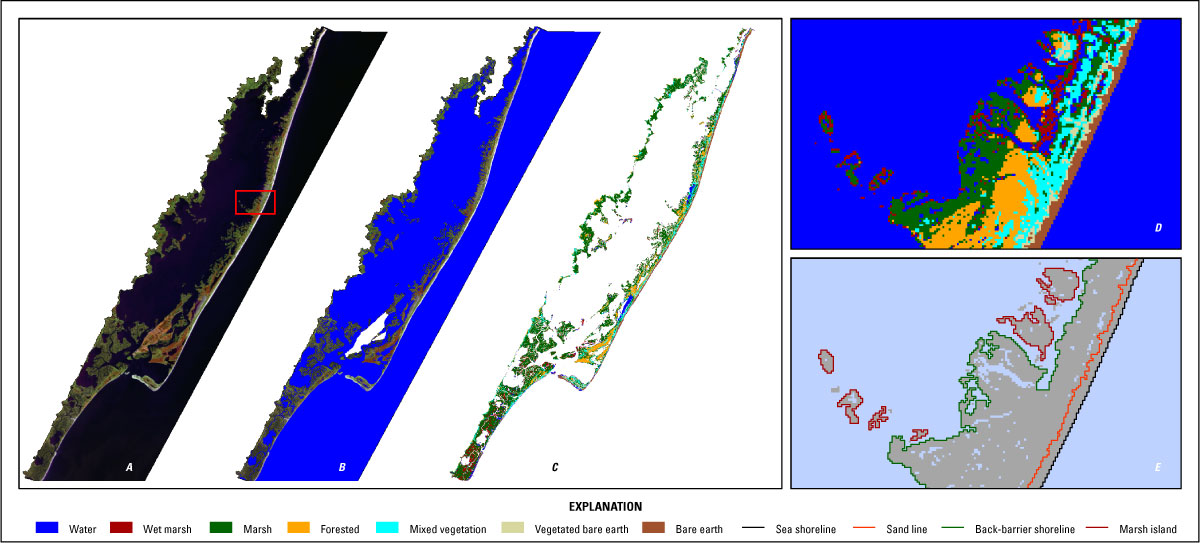Figure 2. Landsat 5 imagery acquired April 28, 1989, illustrates the classification methodology used in this study: (A) Radiometrically corrected, mosaicked image is clipped to study area extent; (B) Unsupervised classification of edge-enhanced image is performed to identify water areas; (C) Water areas from (B) are masked from (A) and unsupervised classification of the remaining pixels are grouped into seven classes (water, wet marsh, marsh, forested, mixed vegetation, vegetated bare earth, and bare earth); (D) Results of (B) and (C) are merged to generate final thematic raster dataset; (E) Line feature classes representing open-ocean, back-barrier, and estuarine mainland shoreline positions and beach/sand-line positions are generated from (D). Red box in (A) indicates extent shown in (D) and (E). [Click image to enlarge]

The “wet marsh” class appears visibly wetter in the Landsat imagery than the surrounding marshes but has a higher spectral reflectance than water areas (fig. 3). In many instances, the marsh surface may be submerged but still be visible due to absorption of the infrared wavelengths. The extent of wet marsh is highly variable and is likely a function of water levels at the time of image acquisition, marsh-surface elevation, and seasonal vegetation changes (Bernier and others, 2006). Persistent extents of wet marsh may indicate areas that will be more susceptible to storm-induced change or submergence by future sea-level rise. The “mixed vegetation” class is a relatively high reflectance class (fig. 4) that likely includes areas of high marsh as well as woody shrub/scrub vegetation. In some areas, land cover noticeably varied between the marsh and mixed vegetation classes depending on image acquisition date. This variability is likely related to seasonal or inter-annual differences in the vegetative growth cycle and density of vegetative type and cover.

Even after using a hybrid classification approach, some areas that were classified as wet marsh in the final thematic raster dataset appeared, upon visual inspection, to include submerged aquatic vegetation and submerged sand flats that would be more appropriately classified as open water. These ambiguities are not consistent through time but most commonly occur in Sinepuxent Bay south of Ocean City Inlet, north of Green Run Bay and Pirate Islands, in impoundments behind Chincoteague Island, and at Chincoteague Inlet. Similarly, in some instances, areas that were classified as water in the final thematic raster dataset were interpreted as wet sand on visual inspection. This most commonly occurs along the narrowest part of Assateague Island south of Ocean COity Inlet, at the Tom’s Cove spit, and along Metompkin Island. Additionally, some near-shore estuarine areas exhibit “speckling” caused by misclassification of isolated higher reflectance pixels within the water body. No manual cleaning of open-water speckling or potentially misclassified pixels was performed.

Sand- and shoreline positions were extracted from the final thematic raster datasets using the Raster to Polygon and Polygon to Line tools in ArcGIS 10.2. The primary sand lines represent the continuous inland extent of sand behind the open-ocean shoreline; lines representing sand extents or vegetation “islands” larger than eleven pixels (about 10,000 square meters [m²]) were also included. Similarly, the primary back-barrier shoreline represents the continuous back-barrier land extent; however, shorelines around back-barrier marsh islands larger than 10,000 m² were also included in the shoreline datasets. Line features were manually edited on the basis of visual comparison with both the original Landsat image and the final thematic raster dataset; for example, classified land areas that were visually interpreted as open water were excluded from the back-barrier shoreline or back-barrier island extents.

Figure 3. Example of wet marsh land-cover class shown on (A) radiometrically corrected Landsat 5 composite image acquired November 26, 2008, and (B) corresponding thematically classified raster dataset. False-color RGB visual display uses bands 4,5,3. [Click image to enlarge]

Figure 4. Example of mixed vegetation land-cover class shown on (A) radiometrically corrected Landsat 8 composite image acquired April 1, 2014, and (B) corresponding thematically classified raster dataset. False-color RGB visual displays use bands 4,5,3. [Click image to enlarge]