Sea-Floor Mapping and Benthic Habitat GIS for the Elwha River Delta Nearshore, Washington

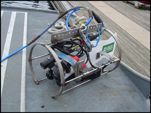
METHODS

Benthic substrate and habitat mapping were conducted with combined interferometric sonar and underwater video-camera system operated from the research vessel R/V Karluk from March 1531, 2005. The cruise reports can be viewed online at http://walrus.wr.usgs.gov/infobank/k/k105ps/html/k-1-05-ps.meta.html and http://walrus.wr.usgs.gov/infobank/k/k204ps/html/k-2-04-ps.meta.html.

Sonar

Sonar data were collected using a 234 kHz SEA Swathplus interferometric sonar. Interferometric sonar imaging provides high-resolution images of the sea floor by recording the intensity of sound reflected off the sea floor (acoustic amplitude). In addition, sea-floor depth data are estimated from the phase difference between seafloor reflections received by spaced receivers. The sonar was mounted on a pole manufactured expressly for use on the R/V Karluk (fig. 2), while the Karluk was navigated on alongshore transects at approximately 4 knots.

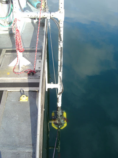
Figure 2. Custom mount for the interferometric sonar on the starboard aft deck of the R/V Karluk.

Sea-Floor Video

Video imagery of the seafloor was obtained on the final 3 days (March 16-18, 2004) of the USGS research cruise aboard the R/V Karluk. The techniques used to characterize the video observations real-time on the boat were consistent with methods described by Anderson et. al. (in press). The objectives of sea-floor video characterization were to: (1) record geologic and biologic characteristics of the sea floor in real-time, (2) ground-truth geophysical data (bathymetry and amplitude) by resolving both common and unique features of the sea floor, and (3) examine regions of transition between different substrate types as suggested in acoustic amplitude data. Video observations were subsequently used to construct maps of substrate type and habitat distribution and to provide a measure of uncertainty in the final products. Thus, video transect locations were selected on the basis of the existence, quality, and complexity of sonar data and on regions of geologic transition and/or biologic significance.

Figure 3. Underwater video sled used to characterize sea-floor features.

An underwater video sled (fig. 3) was towed behind the vessel, at an altitude of 1-3 m above the seafloor. The R/V Karluk was generally drifting during video transects, because the coastal currents were adequate to transport the boat at speeds over 1 knot. Video footage was recorded to digital mini-DV tape and then copied to DVD. Ship position was determined by a CSI Wireless differential geographic positioning system (dGPS). All instrument data were multiplexed through a sub-sea housing and transmitted by the 12-conductor cable to a topside console. Latitude, longitude, height above the seafloor, pitch, roll, water depth, ship speed, ship heading, and Coordinate Universal Time (UTC) were continuously imprinted on the digital video tape while recording. These data were also automatically recorded once per second in a navigational text file. Positional accuracy of the sled relative to the ship's dGPS position varied with water depth, current speed and direction, and conditions. Cable layback was not measured directly but was estimated to be less than or equal to the water depth during the deployments.

Sea-floor characteristics were observed and recorded digitally in real-time at 30 second intervals by a geologist and a biologist watching the towed video. Observations included geomorphology, sediment texture, and biota, and observation codes were entered as "events" in G-Nav navigation software (see acknowledgments) using an "X-Keys" programmable keypad and a Dell Inspiron 8100 laptop computer. Time (UTC), dGPS position, and other ship data for were automatically recorded in the text file each time an observation event was entered. Observations at each event included:

• Primary and secondary substrate type (for example, boulder/cobble, rock/sand, mud/mud).
• Substrate complexity (rugosity).
• Sea-floor slope.
• Benthic biomass (low, medium, or high).
• The presence of benthic organisms and demersal fish.
• Small-scale sea-floor features (for example, ripples, tracks, and burrows).

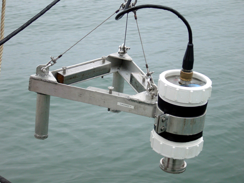
Nearly 9 hours of underwater video were collected and logged real-time in this manner on 18 transects.

Top of Page

Grain-Size Camera

Samples of seafloor grain-size were obtained with an underwater microscope camera (fig. 4) described by Rubin and others (2006) and analyzed by techniques described in Rubin (2004). The camera technique allows for rapid collection of numerous surficial sediment samples and grain-size analysis by autocorrelation spatial statistics on the digital photographs. The camera sampling occurred during the 2004 cruise (K-1-04-PS) during March 21-22, 2004. Eight surficial sediment grab samples were also obtained on these dates for calibration of the images.

Figure 4. Grain-size camera mount used for seafloor sediment sampling.

For each photograph autocorrelation analyses were conducted to measure the average grain size and the distribution of the grain-sizes. The autocorrelation technique was also used to generate a cumulative distribution function of the grain sizes using the Folk and Ward (1957) technique, which was in turn used to compute a number of distribution results, including median, standard deviation, distribution percentiles, sorting, and kurtosis.

Top of Page

Data Processing

The sonar data set covers 19.6 km² and consists of 90 line-files. Sonar bathymetry and amplitude data were processed separately. The bathymetric data were processed using SEA SwathProcessor v2.01. Both the bathymetry and amplitude data output from these software packages were mosaiced into continuous images of the study area using ESRI's ArcGIS v9.1. A horizontal resolution of 1 m was chosen for the bathymetry, and 0.25 m for the amplitude with 8 bit grayscale values proportional to the acoustic amplitude of the sea floor. Processing steps performed on each of these 90 lines were:

Processing backscatter-intensity data

• Imported each raw amplitude line into SonarWiz.MAP 4.
• Used SonarWiz.MAP Sonar File Manager tool to correct the navigation data.
• Manually bottom-tracked each line.
• Applied signal processing functions by setting the Automatic Gain Control, Beam Angle Correction, and projection of sonar data using sensor headings.
• Exported each line as a GeoTiff file.
• Imported GeoTiff file to ArcGIS.
• Converted the GeoTiff files to ESRI GRID format.
• The individual swath grids were mosaiced atop adjacent nearshore swaths sequentially. The nearshore side of each swath was masked to remove far-range and noisy data areas without producing gaps or exposing lower quality data in the adjacent swath when overlain on the mosaic. Where the swaths overlapped the data in the underlying deeper edge of the mosaic were overwritten by the values in the masked swath, values were not averaged where overlap occurred, to preserve data texture.

Processing bathymetry data

• Imported each raw bathymetry file into SEA Swath Processor Real-Time Software System.
• Created a SEA Swath Processor configuration file by inputting motion sensor and GPS adjustment and offset information, such as tides, and sound velocity profiles.
• Altered filter settings at problematic ping numbers.
• Imported the SEA Swath Processor files to SEA Grid Processor software and exported them as ASCII Grid files.
• Converted the ASCII Grid files to ESRI compatible ASCII Grid files using DMagic.
• In ArcGIS, imported lines and converted to ESRI GRID format.
• The individual swath grids were mosaiced atop adjacent nearshore swaths sequentially. The nearshore side of each swath was masked to remove far-range and noisy data areas without producing gaps or exposing lower quality data in the adjacent swath when overlain on the mosaic. Where the swaths overlapped the data in the underlying deeper edge of the mosaic were overwritten by the values in the masked swath, values were not averaged where overlap occurred, to preserve data texture.

Top of Page

Analytical Methods for Sea-Floor Classification

Using the combined video and sonar data, we identified four main sea-floor classes in the study area: hard-rugose (boulder and bedrock reefs), hard-flat (mixed sand to cobble sediment), soft (broad areas of medium sand), and sand waves (patches of coarse sand and shell hash with approximately 1-m wavelength ripples). The area mapped by sonar was classified into seafloor classes using the Supervised Maximum Likelihood Classification tool of the Spatial Analyst extension in ESRI ArcGIS 9.1:

• Seven data layers were coregistered in an ESRI ArcMap Project:

1. Euclidean distance from track line grid

2. Rugosity (derived from mosaiced bathy using the Benthic Terrain Modeling Tool Rugosity Builder (http://www.csc.noaa.gov/products/btm/)

3. Entropy from amplitude at 1-m resolution

4. Homogeneity from amplitude at 1-m resolution

5. Entropy from amplitude at 0.25-m resolution

6. Homogeneity from amplitude at 0.25-m resolution

7. Amplitude at 0.25-m resolution

• Supervisory signatures of covariance for the grids were generated using the above seven layers and ESRI ArcGIS Create signatures tool.
• Four bottom sea-floor classes (soft, mixed, hard, and sand-waves) were output and the output four classes grid was converted to polygons using ArcGIS Grid to Polygons Conversion tool.
• The resulting polygons were further subdivided based on seafloor slope, complexity, and bathymetric depth. The additional Greene and others (1999) attributes Meso/Macrohabitat and Modifier were added based on proximity to video observations. The Greene habitat-code attribute list is outlined below. A detailed description of the process steps can be found in the Habitat_poly Shapefile metadata.
• A Bottom Induration attribute value was assigned to each polygon based on its maximum likelihood class. Sand wave and ripple areas were assigned an induration value of soft, poorly sorted sediment areas were assigned mixed induration value, areas of predominantly boulder and indurated Tertiary glacial deposits were assigned a hard induration value.
• A slope class and bathymetric complexity class were calculated for each polygon by averaging the values of slope and complexity of the cells within each polygon.
• Depth zones were determined by classifying the bathymetry grid to four classes (shown below) and converting it to a polygon shape file. For each habitat polygon, the depth zone assigned was the areal majority bathymetric depth zone value.
• The geologic unit attribute of Tertiary deposits was based on the Washington State Department of Natural Resources, Geologic Map GM-50 (Dragovich and others, 2002).

Top of Page

Interpretation of the processed sonar data and video observations resulted in predictions of benthic habitat distribution in the region. These predictions are distinguished as habitat classification codes that follow the “Deep-Water Marine Benthic Habitat Classification Scheme; Key to Habitat Classification Code for Mapping and use with GIS programs.” (modified after Greene and others, 1999). The Deep-Water Marine Benthic Habitat Classification Scheme is outlined below.

Mega Habitat

Megahabitat Use capital letters (based on depth and general physiographic boundaries; depth ranges approximate and specific to study area).

            A = Aprons, continental rise, deep fans, and bajadas (3,000-5,000 m)

            B = Basin floors, borderland types (floors at 1,000-2,500 m)

            F = Flanks, continental slope, and basin/island-atoll flanks (200-3,000 m)

            I = Inland seas, fiords (0-200 m)

            P = Plains, abyssal (>5,000 m)

            R = Ridges, banks, and seamounts (crests at 200-2,500 m)

            S = Shelf, continental, and island shelves (0-200 m)

sea-floor induration

sea-floor induration - Use lower-case letters (based on substrate hardness).

            h = hard bottom, rock outcrop, relic beach rock or sediment pavement

            m = mixed (hard and soft bottom)

            s =  soft bottom, sediment covered

            Sediment types (for above indurations) - Use parentheses.

                        (b) = boulder

                        (c) = cobble

                        (g) = gravel

                        (h) = halimeda sediment, carbonate

                        (m) = mud, silt, clay

                        (p) = pebble

                        (s) = sand

Meso/Macrohabitats

Meso/Macrohabitat - Use lower-case letters.

            a = atoll

            b = beach, relic     

            c = canyon

            d = deformed, tilted and folded bedrock

            e = exposure, bedrock

            f = flats

            g = gully, channel

            i = ice-formed feature or deposit, moraine, drop-stone depression

            k = karst, solution pit, sink

            l = landslide

            m = mound, depression

            n = enclosed waters, lagoon

            o = overbank deposit (levee)

            p = pinnacle

            r = rill

            s = scarp, cliff, fault or slump

            t = terrace       

            v = depression (flat bassin)

            w = sediment waves

            x = nearshore

            y = delta, fan

            z_# = zooxanthellae hosting structure, carbonate reef

                  1 = barrier reef

                  2 = fringing reef

                  3 = head, bommie

                  4 = patch reef

Top of Page

Modifier

Modifier - Use lower-case subscript letters or underscore for GIS programs (textural and lithologic relationship).

           _a = anthropogenic (artificial reef/breakwall/shipwreck)

           _b = bimodal (conglomeratic, mixed [includes gravel, cobbles and pebbles])

           _c = consolidated sediment (includes claystone, mudstone, siltstone, sandstone, breccia, or conglomerate)

           _d = differentially eroded

           _f= fracture, joints-faulted

           _g = granite

           _h = hummocky, irregular relief

           _i = interface, lithologic contact

           _k = kelp

           _l = limestone or carbonate

           _m = massive

           _p = pavement

           _r = ripples

           _s = scour (current or ice, direction noted)

           _t = heavily bioturbated

           _u = unconsolidated sediment

           _v= volcanic rock

Top of Page

Sea-Floor Slope

Seafloor Slope - Use category numbers.  Calculated for survey area from  x-y-z multibeam data. 

           1          Flat (0-1º)

           2          Sloping (1-30º)

           3          Steeply Sloping (30-60º)

           4          Vertical (60-90º)

           5          Overhang (> 90º)

Top of Page

Sea-Floor Complexity

sea-floor complexity - Use category letters (in caps).  Calculated for survey area from x-y-z multibeam slope data using neighborhood statistics and reported in standard deviation units.

            A         Very Low Complexity (-1 to 0)

            B          Low Complexity (0 to 1)

            C         Moderate Complexity (1 to 2)

            D         High Complexity (2 to 3)

            E          Very High Complexity (3+)

Top of Page

Sea-Floor Depth

Seafloor Depth - Use category numbers enclosed by curly brackets.  Calculated for survey area from  x-y-z multibeam data.

            {1}         Intertidal (<0)

            {2}         Intertidal (<0) – 30m

            {3}         30m 100m

            {4}         100m 200m

            {5}         200m and deeper

Top of Page