Sea-Floor Mapping and Benthic Habitat GIS for the Elwha River Delta Nearshore, Washington

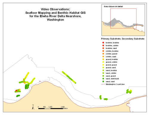
RESULTS

Sea-Floor Features

As described in Sea-Floor Video methods, the presence of benthic organisms and demersal fish were visually observed and digitally recorded in real time. It is important to note that the towed camera is not adept at observing pelagic species, or demersal species that tend to move upward, move quickly, or move away from a location in response to the approach of the camera sled. Ten species of subtidal biota were observed. Of the species of biota that could be successfully recorded, the most common included brown algae, red algae, tube worms, and sponges. Brown algae were mostly found in mixed and sand habitat and seldom in rocky habitat. Red algae were found only in mixed and sand habitat. Sponges and tube worms were found in mixed, sand and sand-waves habitat. The video observation locations and substrate types are shown in Figure 5.

Figure 5. Map of video observations for entire study area. To view a larger version click on the image above.

Top of Page

The majority of the sampled region consisted of relatively uniform sonar amplitude or ripples with crests oriented parallel to the shoreline. Video data was collected in the study area to determine what the substrate type was of this region with both uniform and rippled amplitude. Figure 6 shows the location of the 2 video lines through regions with variable bottom type. Video observations of these lines confirmed that the regions of uniform and rippled amplitude were dominated by sand-gravel grain-sizes, which are shown with light green colors in figure 6. Examples of video imagery in these regions are included in figure 7. Ripples were observed to have wavelengths of approximately 1 to 2 m. For more images of the sea-floor along these video observation lines, please see the hyperlinks in the project available for download included with this report (instructions on viewing hyperlinks in ArcGIS9.x).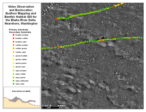

Figure 6. Video observation and amplitude along an area of mixed grain sizes. To view a larger version click on the image above.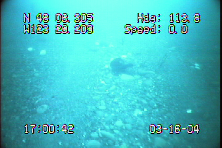

Figure 7. Video observation of sand and gravel sea-floor substrate.

Top of Page

Sonar data also suggested that numerous boulder reefs existed in Freshwater Bay west of the river mouth. Boulders were identified by strong amplitude on the rock front (the rock face toward the sonar sensor) and a region of low amplitude or an amplitude shadow behind the rock. Numerous boulders can be identified in the sonar amplitude image presented in figure 6. Video data was obtained over a few of these boulder reefs, and is shown by the orange and red colors on the two video lines shown on figure 6. An example of the video imagery from a boulder reef is presented in figure 8. For more images of the sea floor along these video observation lines, please see the hyperlinks in the project available for download included with this report (instructions on viewing hyperlinks in ArcGIS9.x).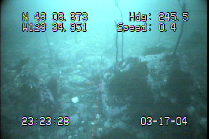

Figure 8. Video observation of boulder sea-floor substrate.

Top of Page

Sonar data also suggested that patches of sand existed in the study area, and that many of these sand waves extended in the across-shore direction. Examples of sand waves are shown in figure 6, and can be identified by the relatively bright patches with widths on the order of 10 to 20 m and lengths from 20 to more than 100 m. Video data obtained over these sand waves revealed that they were entirely sand (dark green in figure 6), in contrast to the mixed sand and gravel that existed in the majority of the survey area. An example of the video imagery from a sand wave is presented in figure 9, which shows a seapen in the sand. For more images of the sea floor along these video observation lines, please see the hyperlinks in the project available for download included with this report (instructions on viewing hyperlinks in ArcGIS9.x).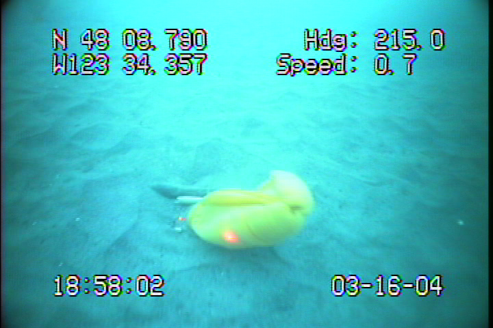

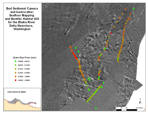
Figure 9. Video observation of sandy sea-floor substrate and seapen.

Top of Page

Immediately to the west of the Elwha River mouth, the sonar data suggested that a broad patch of sand existed approximately 200 to 300 m from the shoreline (fig. 10). This region was sampled using the bed sediment camera, which indicated that grain-sizes were dominated by sand and that grain-size generally coarsened with distance from shoreline (fig. 10).

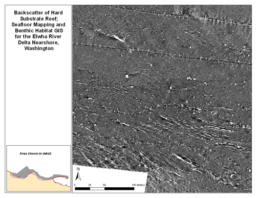
Figure 10. Bed sediment camera and amplitude results from the sand flats near the river mouth. To view a larger version click on the image above.

Top of Page

Sonar data in the center of Freshwater Bay also suggested that a number of hardened or bedrock reefs existed (fig. 11). These features could be identified by parallel structures of alternating high and low amplitude, which suggests geologic bedding features. Unfortunately no video observations were obtained of these features, although geologic mapping suggests that these outcrops may be Pleistocene glacial deposits.

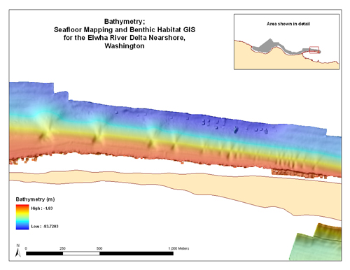
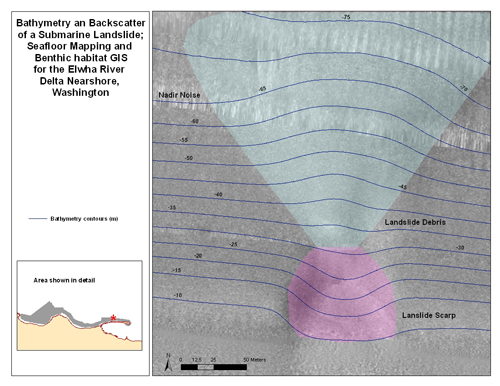
Figure 11. Amplitude of hard substrate reef. To view a larger version click on the image above.

Top of Page

Along the northern side of Ediz Hook a series of submarine landslides were observed. Figure 12 shows the complete set of more than 20 landslides. The slides are largest in the west and decrease in size to the east. For the largest landslides, distinct scarps and debris can be identified in the bathymetric results (fig. 13). The transition from scarp to debris was consistently observed between 30m and 35m water depth.

Figure 12. Bathymetric map along Ediz Hook showing submarine landslides. To view a larger version click on the image above.

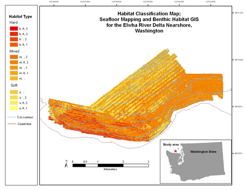
Figure 13. The combines bathymetry and amplitude of the largest observed landslide along Ediz Hook. Pink shading has been placed over the landslide scarp, and blue shading has been placed over the landslide debris. To view a larger version click on the image above.

Top of Page

Habitat Classification

For display of habitat, we produced an image that is colored based on bottom induration, complexity, and slope (fig. 14). Some pixels outside of the bathymetric coverage were classified based solely on acoustic amplitude. These areas are shown in Figure 8 without complexity and slope attributes. Surficial area and percentage of area are shown in table 1. From figure 14 rocky habitat is restricted to the west of the mouth of the Elwha River. Areas of mixed bottom ranging from boulder- to sand-sized sediment predominate in the nearshore out to 20-m water depths. Finer grained sands and possibly mud are more prevalent in deeper water. Though visually complex areas of habitat were noted during video surveying, a standard deviation analysis of the bathymetry data showed that the entire area was within a single Greene and others (1999) complexity class. This is largely a function of the difference in scale between visual observations and the resolution of the sonar bathymetry data. Similarly, the entire study area is within the Shelf megahabitat class of Greene and others, (1999).

Habitat Classification Map

Figure 14. Habitat classification map. To view a larger version click on the image above.

Top of Page

Habitat Class Tabulation

Table 1. Habitation classification. Column one is the Greene and others (1999) Habitat Code. Column two is the definition of the habitat code. Column three is the total area of the habitat type in square meters. Column four is the percent total of the habitat type for the total study area.

Top of Page

Habitat-Classification Accuracy Analysis

• Both sand and sand wave classifications must be accompanied with sand as the primary substrate in the video observations.
• Mixed classification must be accompanied with sand or gravel as either the primary or secondary substrate type, except for when sand was both primary and secondary type.
• Hard classification must be accompanied by cobble or boulder in either the primary or secondary substrate type.

The results of this accuracy assessment are shown in table 2. The accuracy of each of the substrate classes are 62 percent for sand, 67 percent for mixed, 30 percent for hard, and 94 percent for sand waves, with a weighted-average of 64 percent. The uncertainty associated with the classification can be attributed to both poor classification of the sea-floor substrate, and incorrect positioning of the video observations with respect to the sonar data. The latter uncertainty can be attributed to the combined uncertainty in the actual location of the video camera with respect to the research vessel and to the oblique looking angle of the video camera (that is, the camera was not looking straight down at the sea floor). It is difficult to assess the magnitude of each of these elements on the total accuracy assessment of the classification. Including a window of uncertainty for each video observation would produce multiple seafloor classes for each comparison, which would bias the analysis toward success. Thus, the mean accuracy of 64 percent is suggested to be a conservative estimate. The poor accuracy for the hard substrate class (30 percent) is likely due to the small spatial scales of these reefs approximately 10 m (fig. 6) or on the same order of the uncertainty of the video positioning. Hard reefs were often adjacent to sand or sand and gravel, which explains the abundance of these kinds of errors in the uncertainty analysis.

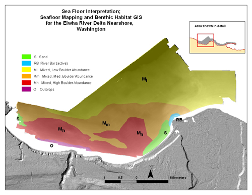
Table 2. The results of the accuracy assessment of the sea-floor substrate classification. Video observation codes are explained in the analytical methods section.

Top of Page

Integration

The results presented above have been integrated into a sea-floor substrate map for the western Elwha River delta presented in figure 15. In general, the entire area that was mapped was observed to have coarse-grained sediment, that is, sand-to-boulders or bedrock outcrops. We defined four substrate classes to characterize the seafloor: sand (S), mixed gravel to boulder (M), bedrock outcrops (O), and river bar (RB); the river bar being the only class without specific sediment grain size information, but rather a specific geomorphic form (a shallow and steep bar). Most of the surveyed region was characterized as having the mixed sediment class (M, figure 15), although there where significant differences in the amount of the largest rocks boulders that are clearly apparent in the sonar backscatter within these mixed areas. Because boulders provide an important substrate for the nearshore habitats, boulder abundances were evaluated by counting individual rocks from the backscatter data in selected regions of mixed sediment class of the survey, resulting in boulder densities of 0 to over 10,000 boulders/km². These differences are represented by three subclasses for the mixed sediment: low, medium and high boulder abundance (M_l, M_m, and M_h, respectively), which are equivalent to average boulder abundances of less than 10 boulders/km², 10-10,000 boulders/km², and greater than 10,000 boulders/km², respectively, as counted from the sonar backscatter data. Although there are clear differences in boulder abundance across the surveyed area, boundaries between subclasses were not always clearly defined, thus the boundaries between the mixed sediment subclasses should be understood as approximate.

The region west of the river mouth generally has many more boulders than the region north and east of the river mouth (fig. 15). This may be due in part to different parent materials for each of these regions, the western portion being derived from sea cliff contributions of glacial till and sedimentary bedrock, and the northern region derived primarily of Elwha River alluvium (Galster and Schwartz, 1990). There is also decreasing boulder abundance with depth, which may be due to boulder burial by sand and gravel with time or differences in parent material.

Two broad regions (>200 m) were dominated by sand, one to the immediate southwest of the river mouth and the other on the far western side of Freshwater Bay (fig. 15). The eastern sand body lies immediately adjacent to the active river mouth bar and offshore of a region in which the littoral sediment has accumulated to a distance greater than 200 m from the sea cliff (as shown by the lidar data; figure 15). Lastly, there is clearly at least 2 km of bedrock outcropping in the central Freshwater Bay within water depths less than 10 m (fig. 15).

Figure 15. Interpreted Sea-floor Substrate map. To view a larger version click on the image above.

Top of Page