U.S. Geological Survey Data Series 675
In general the acquisition hardware for 2008/2009 surveys included four components: a GPS base and GPS rover, a motion sensor (vessel heave, pitch, and roll), and an echosounder. However, some sensors were specific to each vessel based upon hardware configuration. The RV Survey Cat surveyed the areas shoreward of 6 meters (m) water depth while the RV G.K. Gilbert surveyed offshore of 6-m water depth. A portable push buggy with a rigid antenna mount served as the platform to collect shoreline data using a basic kinematic GPS survey.
On the RV Survey Cat, the single-beam transducers are sled mounted and ride on a rail that is attached between the catamaran hulls. During surveying the sled is pulled forward and secured into a position located directly below the GPS antenna (fig. 7). The motion sensor is located along the centerline of the boat in the forward cabin. All hardware component positions on the RV Survey Cat were surveyed using a static total station while the boat was on the trailer and leveled. The base of the transducers served as the reference point. This effort provided millimeter-accuracy for numerical offsets for post-processing.
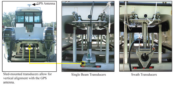
Figure 7. Photographs of the hardware components on the RV Survey Cat. [larger version] |
For the single-beam bathymetry conducted in 2008, depth soundings were recorded at 50-millisecond (ms) intervals using a Marimatech E-SEA-103 echosounder system with dual 208-kHz transducers. Boat motion was also recorded at 50-ms intervals using a TSS DMS-05 sensor. The 2008-2009 swath bathymetry was collected using a SEA SWATHplus-H 468 kHz Interferometric System. Boat motion for the swath came from the CodaOctopus Octopus F190 Precision Attitude and Positioning Systems.
On the RV G.K. Gilbert the transducers were attached to a rigid pole mount with the antennas for both the Ashtech Z-Xtreme receiver and the Octopus F190 located directly above the transducers (fig. 8). For the single-beam bathymetry survey conducted in 2008, the depth soundings were recorded at 20-ms intervals using a Knudsen 320 Bathy Profiler. Boat motion was recorded at 50-ms intervals using a TSS DMS-05 sensor. The 2008-2009 swath bathymetry was collected using SEA SWATHplus-H 468 kHz Interferometric System. Boat motion for the swath came from the Octopus F190 Precision Attitude and Positioning Systems.
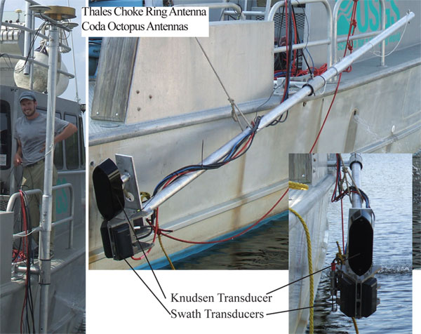
Figure 8. Photographs of the hardware components on the RV G.K. Gilbert. During acquisition the pole is vertical with the Thales choke ring antenna and the Octopus F190 antennas at the top and the transducers at the base with the swath transducers forward and the Knudsen transducer aft. [larger version] |
The single-beam bathymetry on both vessels was acquired using HYPACK MAX version 4.3A (HYPACK, Inc.), a marine surveying, positioning, and navigation software. The data from the GPS receiver, motion sensor, and fathometer were streamed in real time to a laptop computer running HYPACK on a Windows operating system. HYPACK acquisition combines the data streams from the various components into a single raw data file, with each device string referenced by a device identification code and time stamped to the nearest millisecond. The software also manages the planned-transect information, providing real-time navigation, steering, correction, data quality, and instrumentation-status information to the boat operator.
The swath bathymetry on both vessels was collected independently of HYPACK using the acquisition interface of the SEA's SWATHplus software version 3.6 (fig. 9). The position and motion data from the Octopus F190 and the swath transducers were streamed in real time to a dedicated laptop computer.
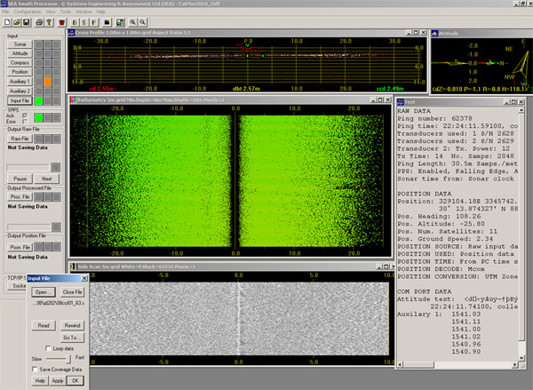
Figure 9. A screen shot of SWATHplus data acquisition and processing interface. [larger version] |
The portable-buggy platform, designed to survey the shoreline, was constructed using simple light-weight, floatable materials and outfitted with beach wheels and a fixed-height antenna mount (fig. 10). A Thales Choke Ring antenna and an Ashtech Z-Xtreme GPS receiver were set to record at 1-s intervals concurrently with that of the local base station. A TSS motion sensor was not used, in anticipation of a gentle sloping shoreface.
Buggy deployment was dictated by availability of staff, weather conditions, travel time, and how well it coincided with the planned bathymetry lines for a respective day. Under optimal conditions the boat would deploy the buggy at the lateral extent of an island. The scientist walking the buggy would survey along the high-water mark (strandline) in order to capture the current outline of the island. This line was then used as a boundary for gridding purposes.
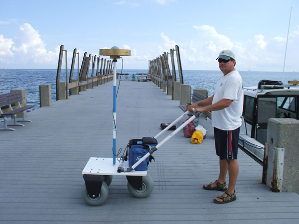
Figure 10. The portable push buggy used to map the island shorelines during the 2008-2009 surveys. The buggy is equipped with a fixed-height antenna mount with a Thales choke ring antenna connected to an Ashtech Z-Xtreme GPS. [larger version] |
The 2008 and 2009 datasets were both processed using differentially corrected external navigation files. However, the point at which the external navigation file was incorporated into the datasets differed between 2008 and 2009. Figure 11 is presented as guidance to facilitate explanation of these detailed processing steps.
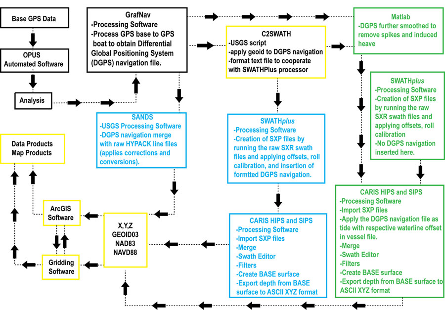
Figure 11. A flowchart indicating steps taken during the post-processing of single beam and swath bathymetry. Blue boxes and green boxes represent 2008 and 2009 processing, respectively. [larger version] |
Establishing the differentially corrected (DGPS) external navigation file began with processing the static GPS data from the primary base station. These data may be processed quickly and accurately through one of the three online submittal services commercially available: (1) Automated GPS-Inferred Positioning System (GIPSY), a service provided by National Aeronautic and Space Administration’s (NASA) Jet Propulsion Laboratory, (2) On-Line Positioning User Service (OPUS), maintained by the National Oceanic and Atmospheric Administration (NOAA) and the National Geodetic Survey (NGS), and (3) Scripps Coordinate Update Tool (SCOUT). The results from these services are put in a spreadsheet for error analysis and averaging. Any sessions that differ from the averaged ellipsoid value by more than 0.05 m are removed. The type of online service used may depend upon the survey logistics, which are defined by the project. For the 2008-2009 bathymetry, the OPUS service results were considered sufficient and produced +/-3.3 cm or less accuracy in the vertical component. These base stations positions, once finalized, were used for processing. The base station position values used for processing are listed on the FACS page under Base Station Logs.
Each base station GPS file was processed to the respective roving vessel or walking buggy GPS file using GrafNav version 8.10, a product of Waypoint Product Group. During this process, steps were taken to ensure that the trajectory produced from the base to the rover was clean and produced fixed positions. This is done through the interpretation and use of graphs, maps, and logs that GrafNav produces for each file. Some simple controls to eliminate poor GPS data at this point included, but were not limited to, excluding data from a satellite flagged by the program as having poor health, eliminating satellite time segments that have had cycle slips, and adjusting the satellite elevation mask angle. From these processes, a single quality-checked, differentially corrected, precise position file at 1-s intervals was created for each vessel or buggy GPS session.
The 2008 single-beam data were processed using the SANDS version 3.92. SANDS uses the time stamp to correlate the external navigation file with the HYPACK line data and performs geometric corrections of the depth values caused by boat motion (pitch and roll). The heave component is not used in SANDS but is more accurately represented by the GPS component (DeWitt and others, 2007; Hansen, 2008; Hansen, USGS, unpub. data, 2009). SANDS also has the option to apply a geoid model and GEOID03 was also applied to the data. The end result was an x,y,z file horizontally and vertically referenced to NAD83 Universal Transverse Mercator (UTM) Zone 16 North (N) and NAVD88 orthometric height.
For processing both the 2008 and the 2009 swath data, the differentially corrected external navigation file (1 position per second) was first reformatted to resemble the SWATHplus position file format and then the GEOID03 correction was applied. This file was then ready for inclusion into the SWATHplus program to create processed swath bathymetry files (SXP). By default SWATHplus uses the navigation string incoming from the positioning and attitude sensor used (the Octopus F190); however, by manually selecting the post-processed differential external navigation file, SWATHplus will substitute the navigation strings accordingly, and the processed files will then be appropriately georeferenced and ready for refinement in other programs.
The 2008 swath data from both survey vessels were processed in SWATHplus version 3.06.04.03. The SWATHplus session files (SXS) for the processing system included the height derivation for the F190, roll calibration offsets, and any sound velocity profile (SVP) casts. The bathymetric filters applied to the data included low amplitude, range, phase configurations, box, quality, along track 1, along track 2, and mean. The SXS files were applied to the acquired data to generate SXP files. The SXP files are horizontally and vertically referenced to NAD83 UTM Zone 16N and NAVD88 orthometric height.
For the 2009 swath data from both survey vessels, the navigation data from the Octopus F190 was included and processed in SWATHplus version 3.06.0. Each swath line included the respective roll calibrations, offsets, and any SVP casts. The filters applied to the data included low amplitude, range, phase configurations, quality, along track 1, along track 2, and mean. The resultant 2009 SXP files were horizontally and vertically referenced to WGS84. At this point the 2009 SXP files do not have the differential external navigation data applied and are only referenced to WGS84. The insertion of the navigation is explained in further detail in the segment Swath Bathymetry Editing.
The files acquired with the shoreline buggy were exported from GrafNav and entered into SANDS, in which they were converted into orthometric heights referenced to GEOID03. The resulting buggy shoreline files contain x,y,z in NAD83 UTM Zone 16N and NAVD88 orthometric height.
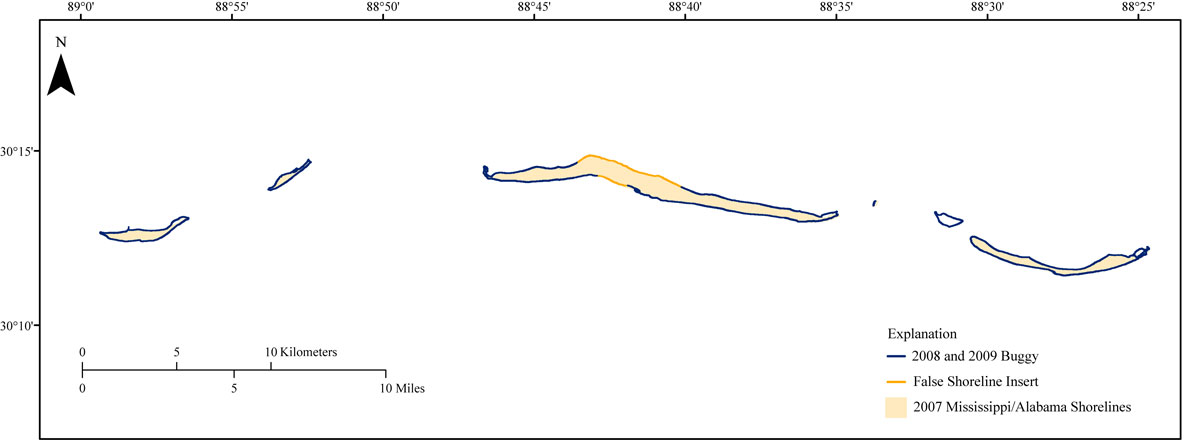
Shoreline buggy data do not exist on Horn Island between the 2008 and 2009 datasets. To fill in this gap a shoreline shapefile was created in ESRI’s ArcMap version 9.3 using the shoreline developed by Morton and Rogers (2009). The Z value for the shoreline file was populated with a static value of +0.50 m. This value was based upon the average of the buggy values at the endpoints of the tracklines (fig. 6). The resulting x,y,z point file was referenced to NAD83 UTM Zone 16N.
The 2008 georeferenced, corrected, and geometrically processed SXP files were imported into CARIS HIPS and SIPS version 7.0 and merged. Each line was edited using Swath Editor to remove stray points and reject any noisy outer beams. When a line displayed some depth consistency along-track, it was possible to use the across-track distance filters to smooth the results. When the files were clean of errant values, a Bathymetry Based on Statistical Error (BASE) surface was created. A BASE surface is a georeferenced image of a weighted-mean surface of the swath data where each node of the surface is based on the uncertainties of the surrounding soundings (CARIS, 2008). A 5-m BASE surface was created and was further reviewed for any questionable data areas that, if found, were edited accordingly and remerged, and a new BASE surface was then recomputed. The depth value from the BASE surface was then exported to American Standard Code for Information Interchange (ASCII) x,y,z format.
The 2009 SXP files for both survey vessels were imported into CARIS HIPS and SIPS version 6.1 with the differentially corrected external navigation files inserted into the 2009 swath bathymetry files. First, the navigation files were smoothed to remove any stray spikes and induced heave, using Matlab version R2007b. Next, the SXP files were imported into CARIS with the heave correction (waterline height) offset in the respective vessel file, and the navigation data were applied as a tide file in CARIS during the merge process. Each line was viewed and cleaned in Swath Editor. The filters applied included depth, beam to beam slopes, across-track distance, and missing neighbors. The files were remerged after any changes occurred during the editing process, a 5-m BASE surface was created, and the x,y,z data were exported in ASCII format for further grid interpretation.
The quality control measures used in SANDS were implemented in swath acquisition and post-processing. Continuous GPS monitoring as described earlier is ongoing throughout the survey. Planned crossing lines are incorporated throughout the survey to validate consistent data acquisition. Crossing lines were surveyed at another time of the day or on a different day from that of the transect lines with the objective to survey across the same area while receiving GPS from different satellite orientations. Also, for the single-beam surveys, bar checks were taken every day to account for any drift in the echosounders. Bar checks test the accuracy of the sonar equipment by placing a metal rod of a know length underneath the transducer and recording the values given by the echosounder. If there is any drift in the values, it is accounted for in SANDS.
In theory, where two bathymetric lines cross, the data values at that point should be equal. If they are not, this could be an indication of inaccurate values or poor data. GPS cycle slips, poor weather conditions, and rough survey conditions may produce poor data. Water-column sound velocity profiles, if collected, were applied to calibrate proper acoustic travel speeds. Using the same base station GPS data to create the differential navigation for both single beam and swath should produce comparable depth measurements at crossing sites independent of the survey type. (that is swath to swath, single beam to single beam, or swath to single-beam lines). If discrepancies were found at the line crossings, the line in error was either statically adjusted or removed. A line in error is considered to have one or more of the following: (1) a segment where several crossings are incomparable, (2) a known equipment problem, (3) known bad GPS data seen in the post-processing steps which may negatively affect the final depth value.
The program used for data editing and gridding was ESRI ArcMap version 9.3 and version 9.3.1. The individual x,y,z data points were plotted in 1-m color coded intervals and overlain over the gridded and contoured surface. Using all three surfaces as guides helps the editor visually scan and find any remaining discrepancies. For example, converging or crossing contour lines indicate problem areas, and deep holes or abnormally shallow zones that appear in questionable areas may indicate false values. Next, the 2008 single beam and swath data were merged into one shapefile. The data were gridded with the ArcMap 3D Analyst Interpolation to Raster using Natural Neighbors at 50-m grid cell size. The data were then contoured using 3D Analyst Surface Analysis at 1-m intervals. The 2009 swath data were gridded and contoured in the same manner and viewed for discrepancies. The 2008 shapefile was merged with the 2009 shapefile to produce one large x,y,z coverage. This coverage was gridded at 50-m cell size and then contoured at 1-m intervals. A raster mask was created to clip the data to the extent of the survey lines.

![]() U.S. Department of the Interior |
U.S. Geological Survey
U.S. Department of the Interior |
U.S. Geological Survey
URL: http://pubsdata.usgs.gov/pubs/ds/675/html/equipment_processing.html
Page Contact Information: GS Pubs Web Contact
Page Last Modified: Monday, 28-Nov-2016 18:39:51 EST
