• Overview
• Installation
• Using CMGTool GUI
• CMGTool Library
• PROSPECT-in-MATLAB
• Acknowledgement
• Reference
• USGS Related Links
• PCMSC Home
• Search PCMSC
• Index

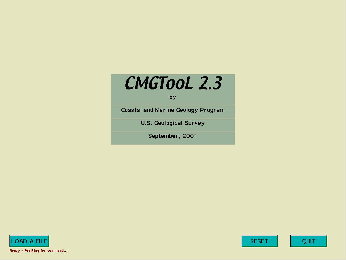
CMGTooL User's Manual

Using CMGTooL GUI

The primary purpose of the CMGTooL GUI is to provide a user-friendly oceanographic data analysis and processing package utilizing MATLAB’s powerful routines for scientists who may only have limited knowledge of MATLAB. CMGTooL GUI is operated almost entirely by mouse-clicks, with keyboard input limited to only few situations. This section describes the main functions of CMGTooL GUI and how these functions are used.

3.1 Starting CMGTooL GUI

The CMGTooL GUI is started by typing cmgtool in the MATLAB Command Window (Figure 1). Notes: all screen-capture images in this document are derived from a MAC. They might look different on either PCs or UNIX computers.

The GUI utilizes both pushbuttons as shown in Figure 2 and a menu bar (not shown) that allows additional functions. The LOAD A FILE button is used to load a NetCDF file. Clicking the RESET button will clear all loaded files from both the GUI window and the MATLAB memory. The QUIT button allows user to quit the program and clear all relevant variables (mainly global variables) from the memory. Two menus, wrapped with square brackets, are added to the built-in MATLAB menu bar. The [Tools] menu allows user to choose between programs that analizing/processing data in theTime Domain (default) or Frequency Domain. After a NetCDF file is loaded, the title of the CMGTooL window will change accordingly depending on user’s selection from the [Tools] menu. The [Help Tips] menu provides brief information for most of the commonly used GUI objects. The help information of the chosen item appears in a textbox at the lower left corner of the window. This textbox disappears when the user clicks anywhere inside the GUI window.

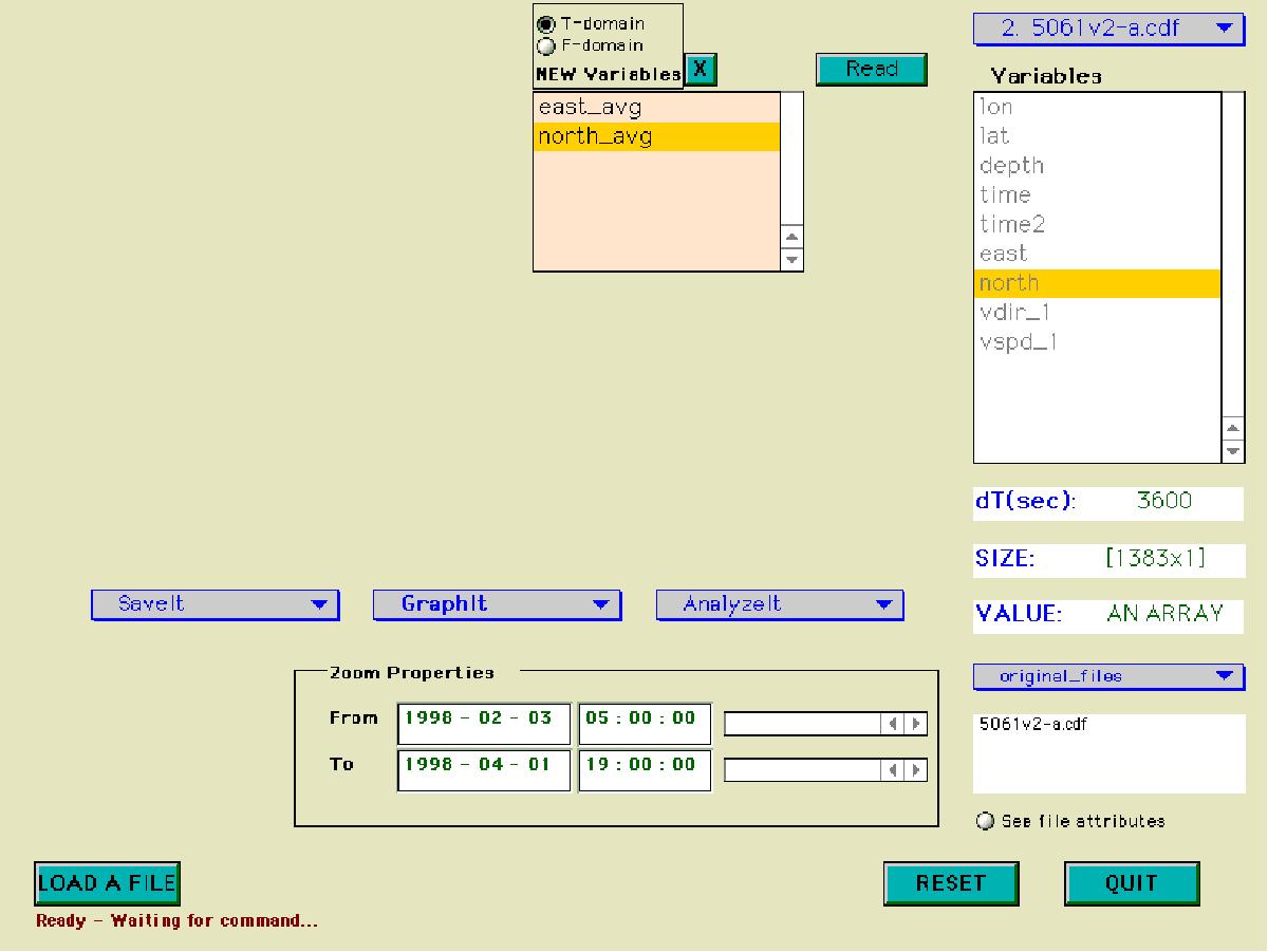
Figure 2. The start-up window of the CMGTooL GUI. If filenames are provided in the typed command, e.g. cmgtool xyz.nc or cmgtool({‘abc.nc’,’xyz.nc’}), this display will not be shown.

Users may also choose to start the CMGTooL GUI with an argument: cmgtool(filename), where filename is a string when there is only one file e.g. ‘5103-a.nc’, or a cellstring when there are multiple files e.g. {‘5103-a.nc’,’5104-a.nc’,’adcp3.cdf’}. The file(s) in the argument will be loaded at the start of CMGTooL. Note: The CMGTooL GUI requires that all NetCDF files must have a time variable named ‘time’ in true Julian days. If the file is EPIC compliant (Soreide, 1997), there should be two time variables (‘time’ in true Julian days and ‘time2’ in milliseconds).

3.2 Loading NetCDF files

Clicking the LOAD A FILE button in Figure 2 will bring in the file selection I/O interface from which users may select a NetCDF file to load. PC and UNIX users may choose to only display files with .cdf (or .nc) suffix. Users will be warned if any error occurrs during file loading. As soon as a file is loaded, The CMGTooL GUI window appears on the screen (Figure 3).

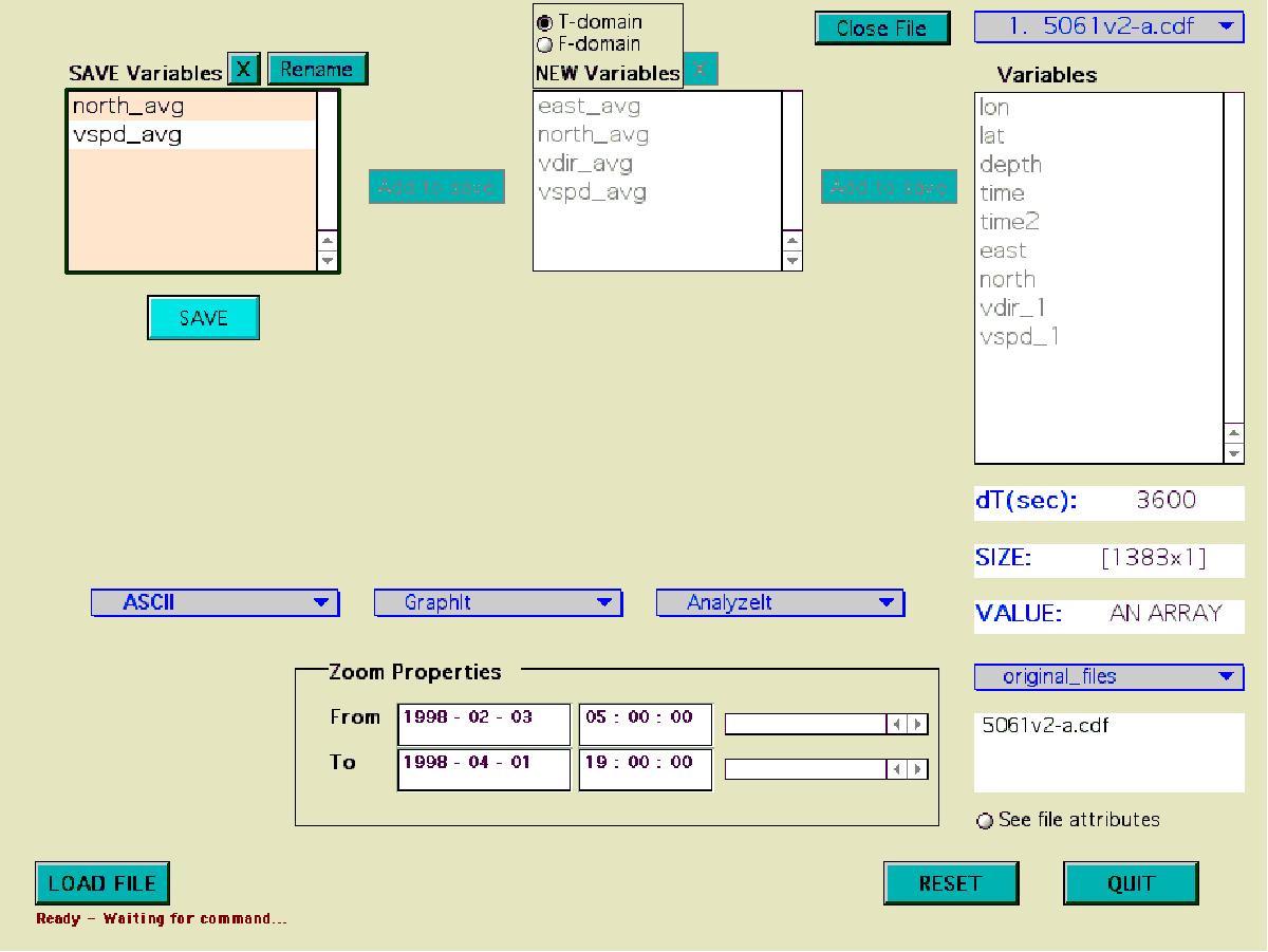
Figure 3. The screen image of a fully-functional CMGTooL GUI.

3.3 The CMGTooL Window

As soon as a file is loaded the CMGTooL becomes fully functional and most GUI objects (pushbuttons, listboxes, popupmenus etc.) are displayed in the CMGTooL window (Figure 3). As many as 9 files can be loaded into one session.

Most GUI objects are self-describing. The popup menu at the upper right corner lists all the loaded files from which users can choose for processing, plotting, or analysis. The Close File push button to the left allows users to close the selected file and remove its variables and attributes from the memory. When a file is chosen, all variables in the file are displayed in the Variables listbox at the right side of the GUI window. The time increment, in seconds, is displayed in the dT textbox below the listbox. The beginning and ending time of the file are displayed in the Zoom Properties frame. The global attributes of the file can now be viewed by selecting from the ATTRIBUTES popup menu. The See file attributes radio button should be in the active state (down position) to view a global attributes. Therefore global attributes can be viewed at any time by pressing the radio button.

When a variable in the listbox is clicked, its size and value are displayed. If the variable is an array, ‘AN ARRAY’ is displayed in the VALUE textbox. The attributes of the selected variable can be viewed by selecting from the ATTRIBUTES popup menu. The data values of a selected variable may be examined by clicking the Read button to the left of this listbox.

The New Variables listbox (Figure 3) is used to store new variables calculated from the analysis methods that will be described later. An X push button is activated when a new variable is clicked and can be used to remove the chosen new variable from the workspace. The time increment, size, and attributes of the new variables are displayed when they are selected. When users click a variable in either listbox, this listbox becomes highlighted with a different background color. The text color in the dT, SIZE, and VALUE textbox also changes when a different listbox is highlighted. The contents of each variable form the New Variables listbox may be examined by clicking the Read button.

The T-domain and F-domain radio buttons above the New Variables listbox allow users to retrieve variables created from either domain without changing to that domain using the [Tools] menu. When T-domain is activated, the New Variables listbox will display the new variables created by the time-domain methods, and vise versa. In another word, users can access the new time-series variables from frequency-domain desktop by activate the T-domain radio button.

The three popup menus in the middle of the window contain the main functions of the CMGTooL GUI. AnalyzeIt allows users to choose from different analyzing methods for processing a variable or variables displayed in both variable listboxes. These variables can be derived from different files. GraphIt allows users to create a variety of plots of the variables. SaveIt allows users to save selected variables into a file that may be one of three formats: NetCDF, ASCII text, and MATLAB binary. The programs listed under the AnalyzeIt and GraphIt change when users switch from Time Domain to Frequency Domain in the [Tools] menu.

3.4 Time-Domain Functions

3.4.1 AnalyzeIt — The time-series analyzing methods

In order to use these methods on time-series data, users are first required to provide input parameters. To input a variable, users can either first choose a variable from either listbox and then click the << Variables button, or directly type the name of the variable in the textbox. The first input method is recommended to avoid typos. After all required input parameters are filled, click the RUN button to execute. Most outputs are new variables that are shown in the New Variables listbox. An attribute of each new variable indicates its origin. Some methods do not create new variables. Instead, the output goes directly to the MATLAB Command Window. So far, the following analyzing/processing methods are implemented in AnalyzeIt.

• Arithmetic: This method allows freehand input of a simple arithmetic formula in the textbox. For example, mylunch = 30*eggs + 2*(chickens./wings), in which eggs, chickens, and wings are variables found in either variable listbox. mylunch is a new variable that will be saved in the New Variables listbox. This method can only deal with variables from a single loaded file plus the new variables. New variables generated from this method carry the ‘_fh’ suffix. (Note — MATLAB syntax (e.g. ‘./’) needs to be used)

• Filter-FILTFILT: This method is mostly used to lowpass time-series data. It call the filtfilt.m from MATLAB’s signal processing toolbox. Sampling frequency and cut-off frequency (both in cycle/day) are required. Users may also choose to resample the filtered time-series by providing a subsample interval (e.g., 6 for every sixth point). Typing all in the input will process all variables in the current file that have the length of the timebase. An error will occur if all variables don’t have the same dimension. New variables generated from this method carry the ‘_filt’ suffix.

• Filter-PL33: This method is used to remove tidal signals from time-series data. Hourly data is required as input. Users may also choose to resample the filtered time-series by providing a subsample interval (e.g., 6 for every sixth point). Typing all in the input will process all variables in the current file that have the length of the timebase. New variables generated from this method carry the ‘_f33’ suffix.

• Rotate: This method is used for vector rotation in a Cartesian coordinate. Counterclockwise angles are positive. New variables generated from this method carry the ‘_r’ suffix.

  Input: U, V

  Output: U_r, V_r

• uv2speed: This method calculates speed and direction from the two orthogonal velocity components (e.g., east and north). Zero degree is true north. New variables generated from this method are spd_EN and dir_EN.

  Input: U, V

  Output: spd_EN, dir_EN

• speed2uv: This method calculate the East and North velocity components from speed and direction. Directions are in degrees (using oceanographic convention, i.e. 0-North, 90-East, 180-South, 270-West). New variables generated from this method are EW_vel and NS_vel.

  Input: spd, dir

  Output: EW_vel, NS_vel

• Average: This method computes the point average of time-series data (e.g. create hourly averaged data from a time-series that is sampled in higher frequency). Typing all in the input will process all variables in the current file that have the length of the timebase. New variables generated from this method carry the ‘_avg’ suffix.

• Subsample: This method is used to subsample time-series data. Typing all in the input will process all variables in the current file that have the length of the timebase. New variables generated from this method carry the ‘_sub’ suffix.

• Merge/Interp: This method carries out two operations: 1) to merge a variable ( or variables) from two or more different files; and 2) to interpolate a variable or variables to a different a different timebase. In the Merge operation, the variables must exist in all files that are being merged. Data gaps or overlaps may be present. The time increments of the files may be different, but the time increment of the merged new variables depends on the time-interval provided by the user. When a variable or file number is entered, the Tstart and Tstop fields are automatically filled. The File numbers and Time interval (sec) are required inputs. Users may also change the Tstart and/or Tstop. In the Interp operation, only the variables from the same file may be interpolated therefore the File numbers field is not needed. Users are required to choose an interpolation method from the popup menu and to provide a new time increment. New variables generated from this method carry the ‘_merg’ suffix.

• Inter-file calc: This method performs arithmetic calculations fo two variables from two different files. At present, only addition and subtraction are implemented. If the time increments of the two files are different, a new timebase with the larger value of the time increments is created for the resultant new variable. New variables generated from this method carry the ‘_f2f’ suffix.

• Principal axis: The method computes the major and minor axis properties from a vector time-series. The principal axes as well as the means are plotted in a figure that also includes the scatter plot and ellipse. There is no new variable output.

• Wind stress: This method calculates wind stress from given wind speed and direction. The program first estimates the wind speed at 10 meter above sealevel using an empirical iteration scheme (Wu, 1980). Then it calculates the East and North components of wind stress. New variables are identified as ‘Wstress.EW’ and ‘Wstress.NS’.

• Bridge: This method fills gaps in a time-series data with linear (for short gaps) or spectral (for long gaps) approach based on user’s instruction. It works extremely well for periodic data (e.g., tide). Typing all in the input will process all variables in the current file that have the length of the timebase. Gap information is printed in the MATLAB Command Window. New variables are identified with a ‘_brdg’ suffix..

• Statistics: This method calculates the error bar of a time-series in addtion to the mean, standard deviation, maximum, and minimum. There is no new variable and all the output is printed in the MATLAB Command Window. Users are required to either provide the Degrees of Freedom (DOF) or to select the value of the autocorrelation scale from a plot, using the mouse pointer. The DOF is length of the record divided by the autocorrelation scale (Emery and Thomson, 1997; Noble and Ramp, 2000). For ADCP data, users are asked to select one bin to be used for DOF estimate. Also, users may choose to run the statistics on a portion of the time-series by setting the start and end times from the sliders or typing in the start and end dates/times in the From and To textbox (Figure 3). Typing all in the variable input textbox will process all variables in the current file that have the length of the timebase. Note: Users may choose to use the subtidal (filtered with Filter-PL33) data to calculate error bars when dealing with hourly data.

• Tidal Analysis: This method employs the T_Tide package (http://www2.ocgy.ubc.ca/~rich) to perform the Forman tidal analysis (Forman, 1978). If there are two entries in the Variables input field, a complex time series (U+iV) is formed and tidal analyses are performed on this complex data. In addition to filling the Variables field, users may also need to fill the Tstart and Latitude fields (using the format given) for node correction. No new variables are produced. All outputs are displayed in the MATLAB Command Window. They include frequency of tidal constituents (cph), constituent major and minor axes, 95% confidence intervals for major and minor axes, ellipse orientations (degrees), 95% confidence intervals for ellipse, constituent phases (degrees relative to Greenwich), and 95% confidence intervals for phase. Users can choose to output the O1, K1, M2, and S2 only. A plot is also displayed to compare the original and predicted values.

3.4.2 GraphIt — Graphic presentation of time-series data

This popup menu contains the functions to make plots or displays. Users are first required to provide input parameters. To input a variable, users can either first choose a variable from either listbox and then click the << Add Var. button (the name of the button might be different for different plots) button, or directly type the name of the variable in the textbox. The first input method is recommended to avoid typos. Using the [Save As] menu that is added to the MATLAB default menu of each plot, the plots or displays may be saved in different graphic formats (e.g. JPEG, POSTSCRIPT, ILLUSTRATOR), or sent directly to a printer. The following plot types have been implemented:

• Time-series plot: Users can plot time-series data into as many as 4 panels (subplots). Each panel may have one or multiple variables that can come from different files (Figure 4). To make a vector (stick) plot, use square brackets around the two velocity components, e.g. [U, V]. For most variables the Title and Ylabel fields are automatically filled, but users may change them if desired. Users have an option of turning the legend on and off. After the initial plot is created, users may change the Ylim (y-axis limits) for each subplot. Users may also zoom in on the plot by adjusting the sliders or typing in the date/times in From and To textboxes inside the Zoom Properties frame. When plotting ADCP variables, users are asked to input the number of bins whose records are to be plotted. Normally a one-panel plot is recommended for an ADCP variable. If users need to plot multiple variables, but in the same bin, then multiple-panels should be used and each variable should be in a separate panel. For burst-type data such as ADVs and Electro-magnetic current meters, users are asked to provide the burst number(s) to be plotted. The starting time of each burst is shown at the lower left corner of each subplot, and the x-axis showe the number of seconds from the start of each burst. In each subplot, users may use the right mouse button (Option + click for Macintosh) to change line colors or line types. An example of time-series plot is shown in Figure 5.

Figure 4 (114K)

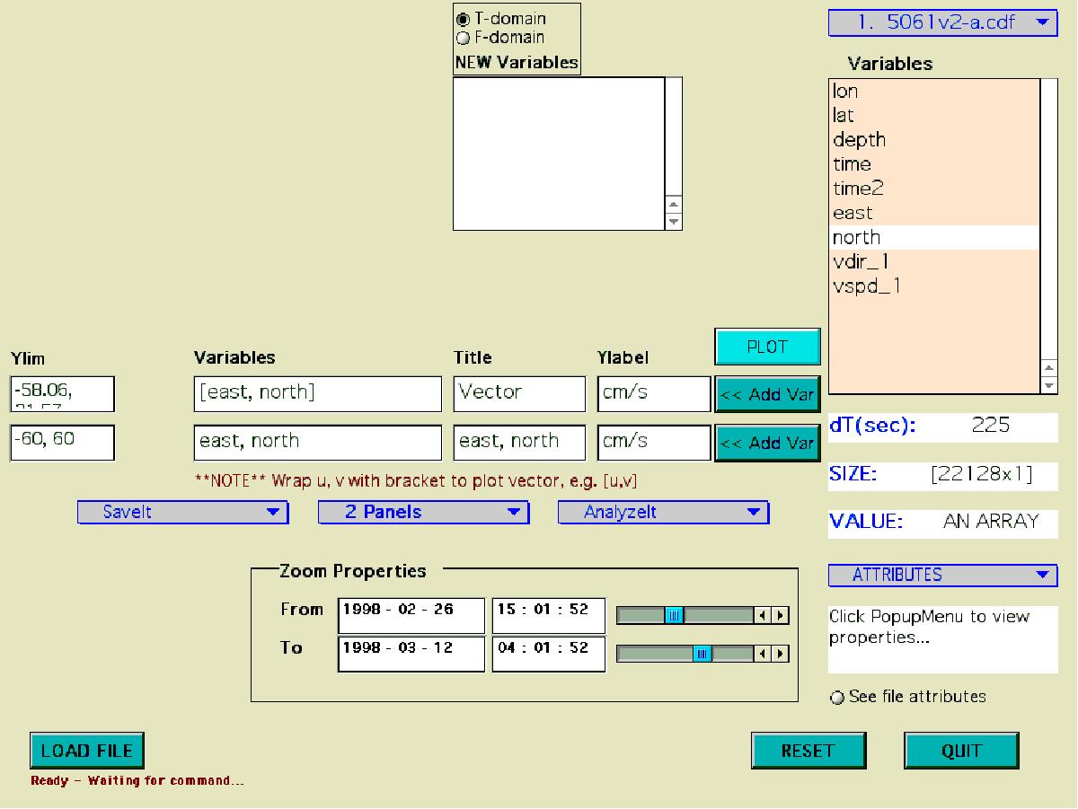
Figure 4. The CMGTooL GUI window that shows the process of plotting a time-series data. The two panels have the same two variables (east and north) from the Variables listbox. But the variables in the top panel are wrapped by square brackets to have a stick plot. Notice that the sliders have been adjusted in order to zoom in the plot.

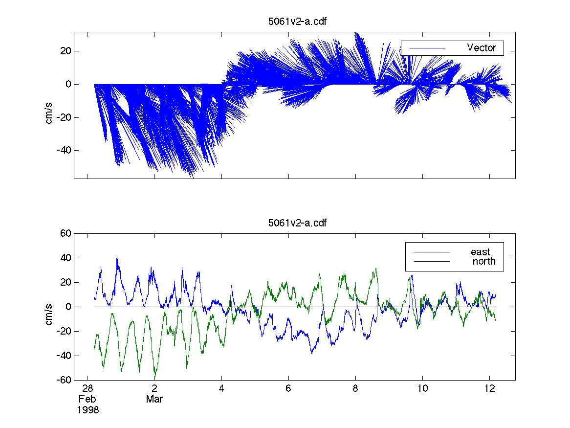
Figure 5. The time-series plot that is created from the settings shown in Figure 3. The lower panel shows the lineplot of the two velocity components. The top panel is the vector (stick) plot of the same time-series.

• Scatter/Progressive Vector plots: Scatter plots are very useful in determining the tidal ellipse and as well as the principal axis of winds or tidal/subtidal currents. Users can choose to plot the ellipse only without the data points. The axes limits can also be changed. The program requires a vector input (East and North components). If the time-series is too long only a portion of the data points are plotted for graphic clarity. The properties of the principal axis are also plotted (Figure 6). The Progressive Vector plots display the history, in a spatial sense, of a time-series vector (Figure 6). Time intervals are also calculated and marked on the plot. It also requires a vector input (e.g. the East and North components).

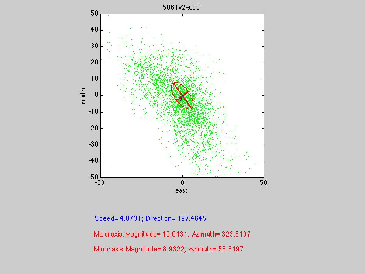
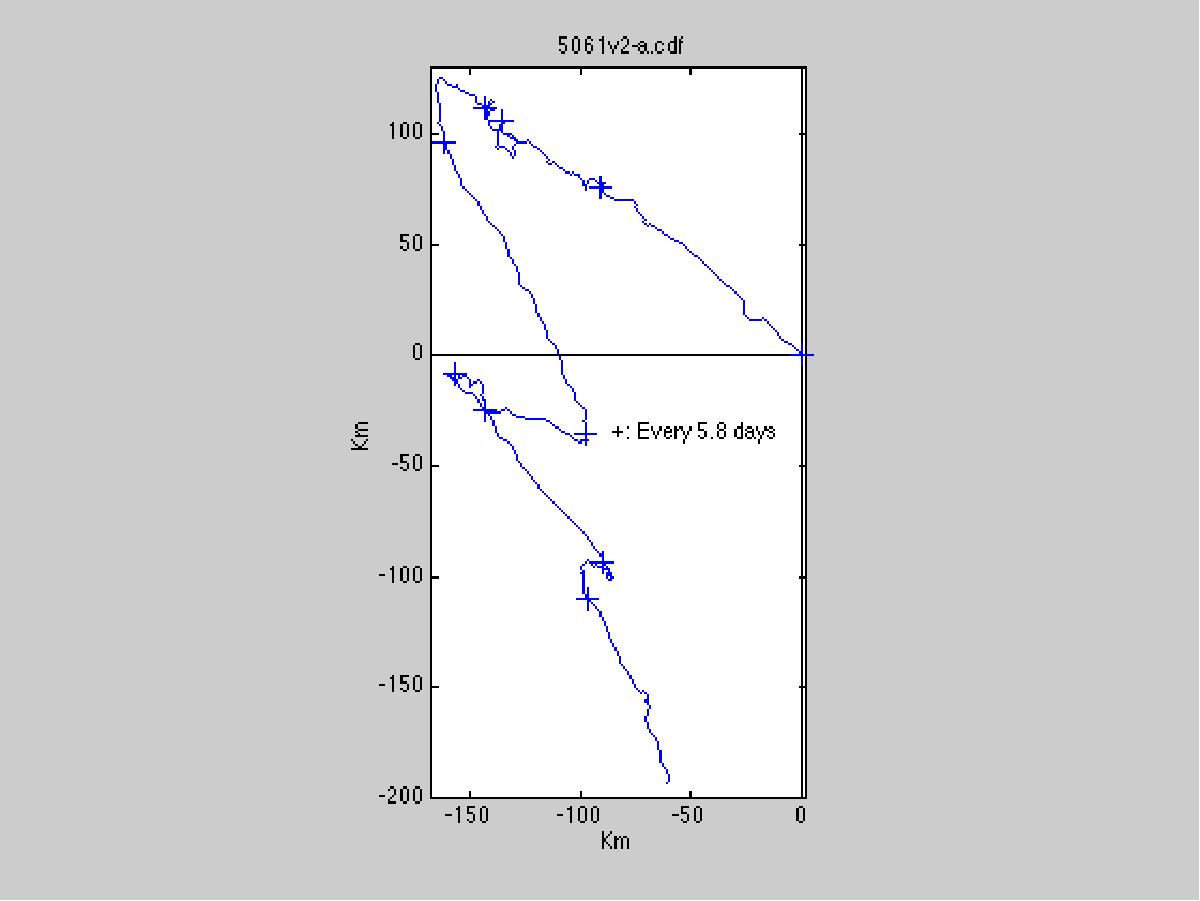
Figure 6. Examples of a scatter plot (left) and a progressive vector plot (right). The principal axis ellipse and its parameters are also shown in the scatter plot. In the progressive vector plot, the ‘+’ symbols are time markers.

• ADCPVIEW: This is a tool to examine ADCP data whose dimension must be [a x b] and b>1 (Figure 7). Required inputs are the two orthogonal, horizontal components of the ADCP measurements. Users may select to display [u,v] or [speed, direction]. From the popmenu a the lower right corner users can set the time span of the display to 1, 3, 7, and 30 days or the whole record. Use the slider to change the time segment of the display. Click anywhere in either image to get vertical profiles of the data at that specific time, these profiles are plotted in the left side of the window. The date, time, and ensemble number are displayed below the profile plots. Use <<Prev. and Next>> buttons to move one ensemble at a time.

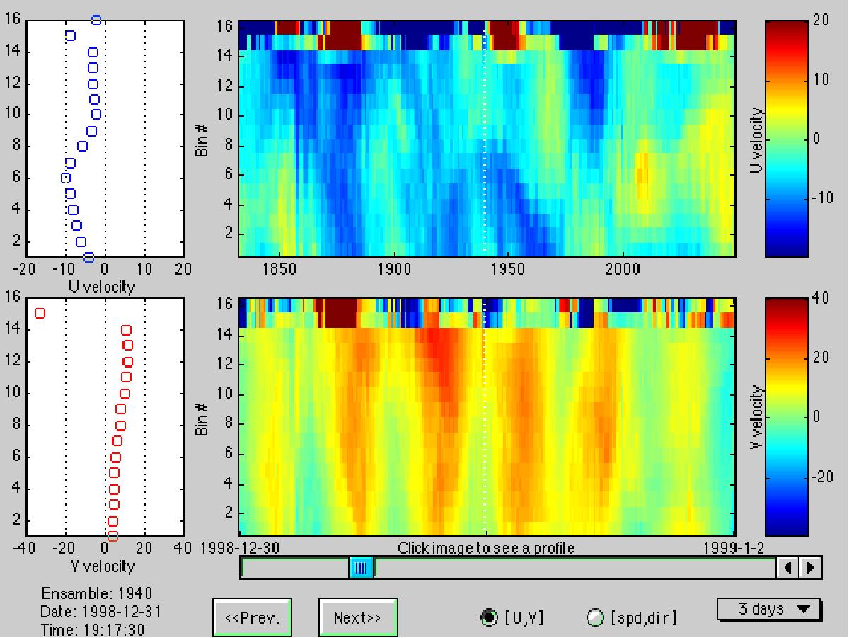
Figure 7. An ADCPVIEW screen shot. The scales of the color images are shown in the two color bars to the right. Note that the top two bins of this particular data are not reliable due to water surface scattering.

• Histogram: This creates a histogram plot of time-series data (Figure 8). Users have options of plotting one or multiple variables at a time. There are 20 bins (default) in the horizontal axis but this can be changed by user. When plotting ADCP or ADV data, only one variable may be plotted at a time, and users are asked to provide the bin/burst number that is to be plotted.

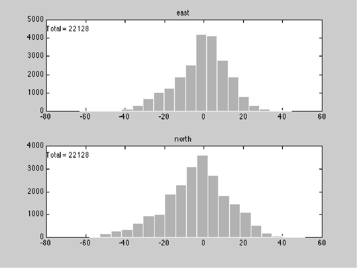
Figure 8. Example of a histogram plot. The total number of point is printed at the upper left corner of each panel.

• Polar: This creates a polar plot (Figure 9). The input data can be: 1) an orthogonal pair (U, V); or 2) the speed and direction of the time-series measurements. The oceanographic convention (North=0, East=90, South=180, West=270) is used.

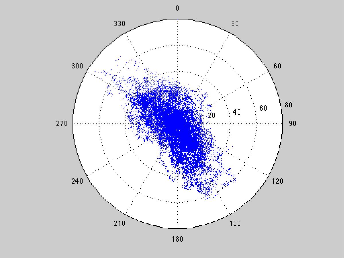
Figure 9. Example of a polar plot of the same data shown in Figure 8.

3.4.3 SaveIt — Saving variables into new files

The SaveIt popup menu provides users with three formats of saved files: ASCII, MATLAB, and NetCDF. A listbox named SAVE Variables is displayed at the upper left corner along with five push buttons that allow user to add variables into the listbox, remove variable from the listbox, rename variables, and save the variables into a file. ASCII allows users to save variables into text files. Some file and variable attributes are saved into the headers of the text file. The first six columns hold the time variable in [yyyy mm dd hh mm ss] format, with the variables saved in subsequent columns. Choosing MATLAB allows users to save variables into a MATLAB binary (*.mat) file, and NetCDF allows users to save variables into a NetCDF file. Variables from different files that have different data lengths or time increments can be saved into a single output file. However, users are asked to form a common timebase using either the largest or smallest time increment; and the variables are interpolated to the common timebase if necessary. Users are also asked if they need to save a certain time range instead of the whole record (default). If the answer is yes then users are lead back to the CMGTooL window to use the sliders to specify the time range. The time variable(s) is always automatically saved. ADCP or ADV variables that are matrices cannot be saved into NetCDF files on Macintosh computers owing to technical difficulties. Figure 10 shows the CMGTooL window when ASCII is chosen.

Figure 10. The screen shot of the GUI when an ASCII file is being saved. Variables from both the Variables and New Bariables listboxes can be saved together into a new file. After the SAVE button is clicked the first time, users can change the time range from the sliders that are now actived.

3.5 Frequency-Domain Functions

CMGTooL always starts in Time Domain. Use the [Tools] menu to switch to Frequency Domain. The title of the CMGTooL GUI window changes to CMGTooL — Spectral after the domain is switched. The new variables that have been saved in the Time Domain will be hidden. The entries under the AnalyzeIt and GraphIt also change accordingly.

3.5.1 AnalyzeIt — Spectral analysis of time-series data

In order to use these methods on time-series data, users are first required to provide input parameters. To input a variable, users can either first choose a variable from either listbox and then click the << Variables button, or directly type the name of the variable in the textbox. The first input method is recommended to avoid typos. After all required input parameters are filled, click the RUN button to execute. The output spectra are saved as new variables in the New Variables listbox. An attribute of each new variable indicates its origin.

Spectrum is the only method in the AnalyzeIt popup menu. This function is used to estimate auto- and cross-spectrum of the variable(s). For cross-spectrum, the two variables must be enclosed in the square brackets, e.g. [var1, var2], in the variable field (Figure 11). In order to run spectra on a new variable that was created in the Time Domain, users need to click the T-domain radio button to have those variables displayed in the New Variables listbox. The four parameter fields on the left are editable textboxes. The Window and Detrending popup menus provide users with different options of windows (e.g. Hanning, Cosine, etc) and detrending methods. Auto-spectrum is identified by the ‘_spec’ suffix in the new variable name and has a dimension of [a x 5]. Cross-spectrum is identified by the ‘_specx’ suffix and has a dimension of [a x 19]. When a spectrum variable is highlighted in the New Variables listbox, users can read the cross-spectral data, including auto-, co-, quad-spectra, transfer function, coherence, etc. by clicking the Read button. Users can read only a specified period range by changing the values in the MinMax Pd textbox. If the Band Average checkbox is on, the displayed spectra is band-averaged based on the default averaging scheme: [1 40; 2 5; 5 6; 10 30; 20 15; 50 6; 100 30; 200 15; 500 6]. That is, the first 40 bands are not averaged, the next 5 bands are 2-point averaged, the next 6 bands are 5-point averaged, etc. After the Read button is clicked, users can also click the Hardcopy button to load the spectra data into MATLAB's default text editor. Users need to change the font size to 7 in order to fit the data into the width of a Letter size paper. The font size can be changed from the Edit menu (Edit > format…) of the text editor. After the font is changed, the data can be sent to the printer.

Auto-spectra can also be estimated from ADCP variables. Its dimension is in a form of [a x 5 x b] where b is the number of bins. Cross-spectrum for ADCP variables are not available, but under development.

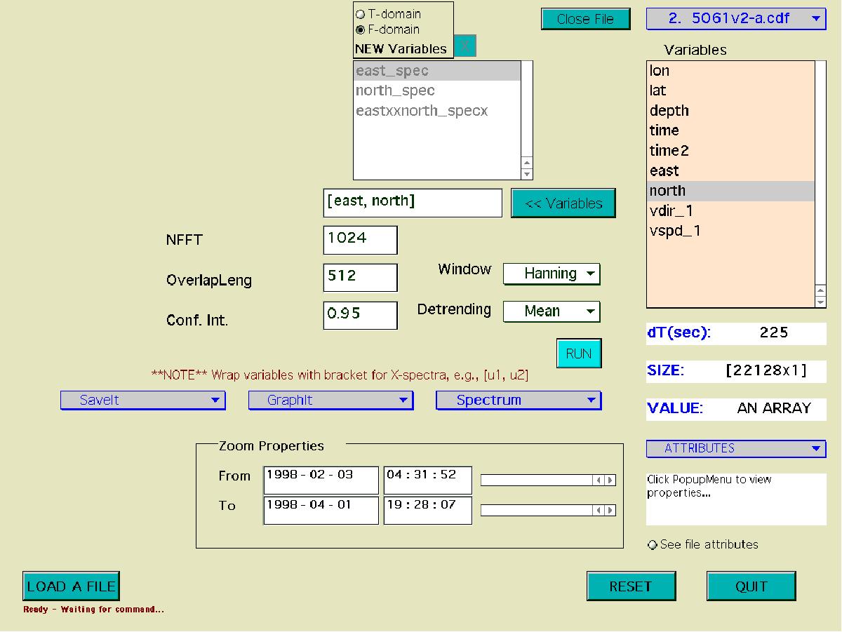
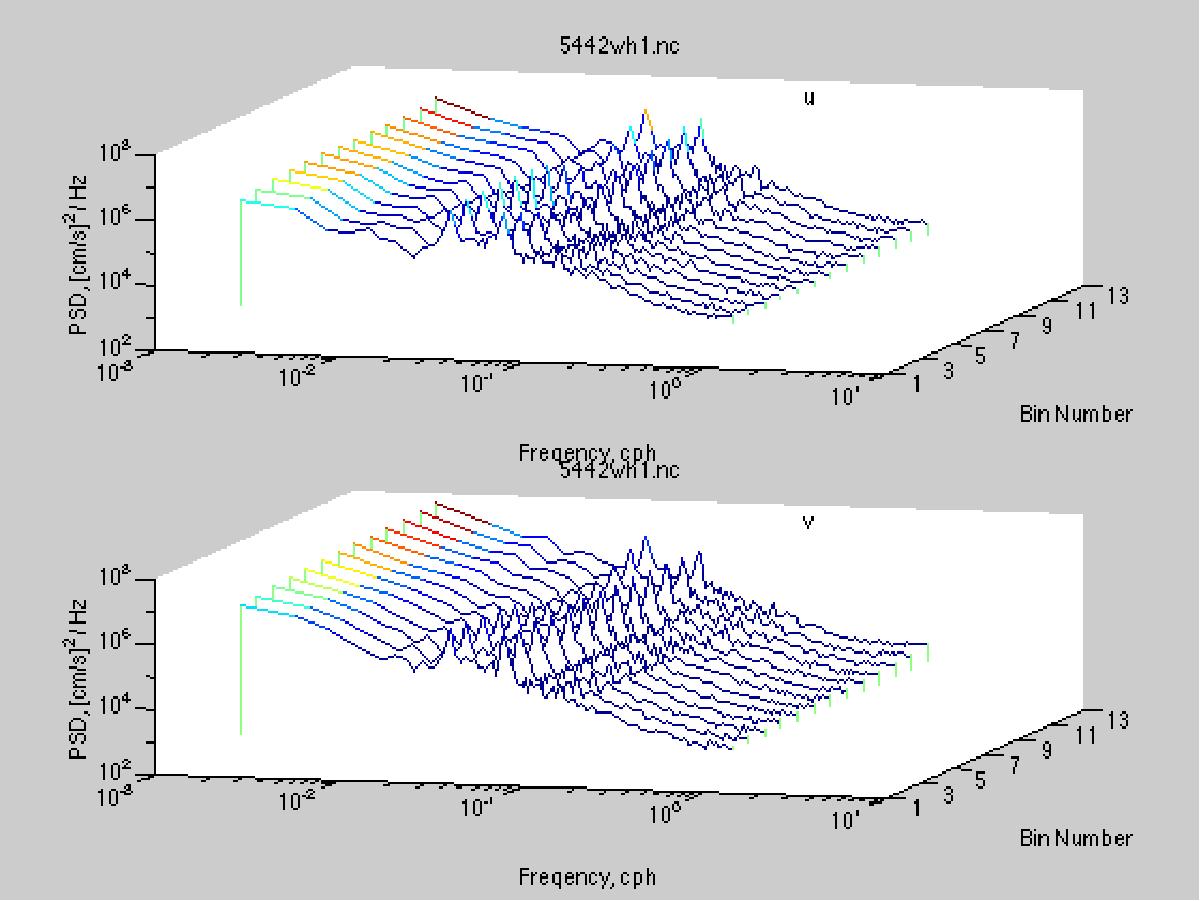
Figure 11. The screen shot of the CMGTooL GUI window in which the cross-spectrum of two variables (east, north) is to be computed when users click the RUN button.

3.5.2 GraphIt — graphic presentation of spectra

GraphIt is used to plot spectral variables. Users may choose from LogLog, SemiLogx, SemiLogy, Linear, or Variance-preserving plots. The last plot type can only be used on auto-spectra only. Users also have the option of plotting band-averaged or unaveraged spectra. The frequency range of the plot may be changed. When plotting a cross-spectra, the auto-spectra, clockwise/anticlockwise spectra, phase, and coherence are plotted in 4 different subplots (Figure 12). When plotting auto-spectra of ADCP data, the spectra are displayed as a 3-D waterfall plot if the spectra are from more than two ADCP bins (Figure 13). Users can choose which bin(s) are to be plotted.

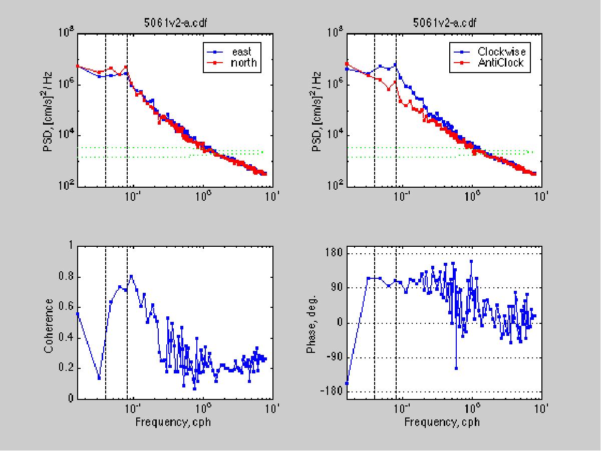
Figure 12. Example plot of a cross-spectrum. The auto spectra, rotary spectra, phase and coherence are plotted in 4 separate subplots.

Figure 13. The waterfall plots of the auto spectra computed from an ADCP time-series data.

3.5.3 SaveIt — Saving variables into new files

Spectral data can only be saved into ASCII or MATLAB format. NetCDF format has not been implemented in the current version. See Figure 10 for instructions of putting variables into the Save Variables listbox.

Any use of trade, product, or firm names is for descriptive purposes only and does not imply endorsement by the U.S. Government.

Suggested citation:

Xu, Jingping, Lightsom, Fran, Noble, Marlene A., Denham, Charles, 2002, CMGTooL user's manual: U.S. Geological Survey Open-File Report 02-19, https://pubs.usgs.gov/of/2002/0019/.

U.S. Department of the Interior
SALLY JEWELL, Secretary

U.S. Geological Survey
Suzette M. Kimball, Acting Director