Open-File Report 02-227
These data were generated from stream-sediment and soil samples collected during the National Uranium Resource Evaluation (NURE) Hydrogeochemical and Stream Sediment Reconnaissance (HSSR) program and reanalyzed during the Winnemucca-Surprise, Malheur-Jordan-Andrews, and Humboldt resource assessments, and from chemical analysis of new samples collected during the Malheur-Jordan-Andrews and Winnemucca-Surprise resource assessments. Samples were collected in all or parts of 17 1° x 2° quadrangles in southeastern Oregon, southwestern Idaho, northeastern California, and, primarily, in northern Nevada.
Samples collected and analyzed under the NURE HSSR program provided incomplete information about the multielement geochemistry of the northern Great Basin. For example, figure 2, below, shows two grids (interpolations) of sample analyses for arsenic from HSSR analyses (left) and from the current data (right).
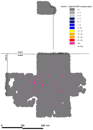
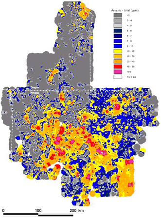
Figure 2.-grid of old NURE arsenic analyses (left), and grid of new arsenic analyses (right).
Lack of a consistent analytical protocol during the NURE HSSR program led to numerous problems for anyone interested in using these data. Sampling and analysis protocols are outlined in data quality. Table 1, below, outlines the labs responsible for samples within our study area.
Table 1.-Summary of labs collecting and chemically analyzing NURE samples within the study area (Acme = Acme Analytical Laboratories Ltd., LLL = Lawrence Livermore National Laboratory, SRL = Savannah River Laboratory, USGS = U.S. Geological Survey, USML = US Mineral Laboratories. Carlson and Lee, in press; Folger, 2000; King and others, 1996; Smith, 2000). (CLICK HERE to download this file (245 KB) in Microsoft Excel format.)
| Quad | Samples Collected By | # Samples Collected | Samples Analyzed By | ||
| Stream-Sediment | Soil | Miscellaneous* | |||
| Adel | SRL | 7 | 814 | 5 | USGS |
| Alturas | USGS | 115 | USGS | ||
| Baker | SRL and USGS | 369 | USGS | ||
| Boise | SRL | 15 | 650 | 41 | USGS |
| Burns | USGS | 125 | USGS | ||
| Canyon City | USGS | 35 | USGS | ||
| Elko | SRL | 155 | 360 | Acme and USML | |
| Ely | SRL | 325 | Acme and USML | ||
| Jordan Valley | SRL | 1 | 603 | 12 | USGS |
| Lovelock | LLL contractor and USGS | 926 | USGS | ||
| McDermitt | LLL and SRL | 85 | 1,237 | 7 | Acme, USGS, and USML |
| Millett | Bendix Field Engineering Corp. (under LLL) | 1,078 | Acme and USML | ||
| Reno | LLL, SRL, and USGS | 156 | 137 | USGS | |
| Tonopah | LLL contractor and USGS | 41 | Acme and USML | ||
| Vya | SRL and USGS | 1,053 | 170 | USGS | |
| Wells | LLL and SRL | 1,082 | Acme and USML | ||
| Winnemucca | LLL contractor and USGS | 473 | 184 | Acme, USGS, and USML | |
Many of the data recently analyzed during the Winnemucca-Surprise, Malheur-Jordan-Andrews, and Humboldt mineral resource assessments are qualified. That is, they are reported as less than a lower limit of determination (LLD), or as not detected. In order to permit the construction of continuous grids and to facilitate interpretation, we made substitutions for these qualified values. This process was complicated by the fact that the lower limit of determination for several elements is different among the data from the three project areas. In general, our goal was to use a substitution value that was between half and two-thirds of the LLD. The substitutions we used are presented in table 2 (below).
Table 2.-Lowest-detectable or minimum-reported values for each element, by study, in the northern Great Basin dataset. (AA = graphite furnace atomic adsorption; ICP-40 = a total analysis method that analyzes 40 elements simultaneously and involves dissolving a sample in a series of acids and analyzing the resultant solution by Inductively Coupled Plasma-Atomic Emission Spectrometry; ICP-Partial = partial dissolution of samples by weaker acid digestions and an organic extraction, allowing for 10 to 15 trace elements to be determined simultaneously; ppm = parts per million. Briggs, 1996; Motooka, 1996; O'Leary and Meier, 1996.) (CLICK HERE to download this file (23 KB) in Microsoft Excel format.)
| Element | Symbol | Method | Lowest-Detectable or Minimum-Reported Values (by study) |
Units | Substituted Value |
# of Qualified Values |
||
| Humboldt | Winnemucca-Surprise | Malheur-Jordan-Andrews | ||||||
| silver | Ag | ICP-40 | 0.5 | 2 | 2 | ppm | 1 | 10,142 |
| silver | Ag | ICP-Partial | 0.012 | 0.067 | 0.067 | ppm | 0.04 | 5,844 |
| aluminum | Al | ICP-40 | 0.82 | 0.69 | 1.9 | percent | none | - |
| arsenic | As | ICP-40 | 5 | 10 | 10 | ppm | 3 | 5,149 |
| arsenic | As | ICP-Partial | 0.86 | 0.67 and 1 | 0.67 | ppm | 0.5 | 586 |
| gold | Au | AA | 0.00001 | 0.002 | 0.002 | ppm | 0.001 | 7,722 |
| barium | Ba | ICP-40 | 92 | 26 | 35 | ppm | none | - |
| beryllium | Be | ICP-40 | 1 | 1 | 1 | ppm | 0.5 | 1,040 |
| bismuth | Bi | ICP-Partial | 0.019 | 1 | 0.67 | ppm | 0.5 | 9,760 |
| calcium | Ca | ICP-40 | 0.13 | 0.2 | 0.7 | percent | 0.01 | 1 |
| cadmium | Cd | ICP-40 | 0.4 | 2 | 2 | ppm | 1 | 9,404 |
| cadmium | Cd | ICP-Partial | 0.019 | 0.5 | 0.05 | ppm | 0.2 | 3,893 |
| cerium | Ce | ICP-40 | 10 | 4 | 11 | ppm | none | - |
| cobalt | Co | ICP-40 | 2 | 2 | 3 | ppm | 1 | 22 |
| chromium | Cr | ICP-40 | 6 | 1 | 6 | ppm | 0.5 | 4 |
| copper | Cu | ICP-40 | 2 | 3 | 5 | ppm | 1 | 1 |
| copper | Cu | ICP-Partial | 1.28 | 1 | 4.1 | ppm | 0.01 | 1 |
| iron | Fe | ICP-40 | 0.38 | 0.21 | 1.1 | percent | none | - |
| gallium | Ga | ICP-40 | 1 | 4 | 8 | ppm | 2 | 2 |
| potassium | K | ICP-40 | 0.34 | 0.17 | 0.33 | percent | none | - |
| lanthanum | La | ICP-40 | 5 | 4 | 7 | ppm | none | - |
| lithium | Li | ICP-40 | 5 | 6 | 7 | ppm | none | - |
| magnesium | Mg | ICP-40 | 0.03 | 0.12 | 0.24 | percent | none | - |
| manganese | Mn | ICP-40 | 82 | 130 | 220 | ppm | none | - |
| molybdenum | Mo | ICP-40 | 2 | 2 | 2 | ppm | 1 | 7,014 |
| molybdenum | Mo | ICP-Partial | 0.204 | 0.08 | 0.12 | ppm | 0.05 | 21 |
| sodium | Na | ICP-40 | 0.07 | 0.1 | 0.3 | percent | 0.01 | 1 |
| niobium | Nb | ICP-40 | 2 | 4 | 4 | ppm | 2 | 35 |
| nickel | Ni | ICP-40 | 2 | 2 | 4 | ppm | 1 | 10 |
| phosphorous | P | ICP-40 | 0.012 | 0.008 | 0.01 | percent | none | - |
| lead | Pb | ICP-40 | 5 | 4 | 4 | ppm | 3 | 255 |
| lead | Pb | ICP-Partial | 3.11 | 1.1 | 2.2 | ppm | 0.5 | 4 |
| antimony | Sb | ICP-Partial | 0.095 | 0.67 and 1 | 0.67 | ppm | 0.5 | 4,750 |
| scandium | Sc | ICP-40 | 1 | 2 | 3 | ppm | 1 | 5 |
| tin | Sn | ICP-40 | 2 | 5 | 5 | ppm | 2 | 7,851 |
| strontium | Sr | ICP-40 | 33 | 29 | 70 | ppm | none | - |
| thorium | Th | ICP-40 | 2 | 4 | 4 | ppm | 2 | 429 |
| titanium | Ti | ICP-40 | 0.04 | 0.03 | 0.13 | percent | 0.01 | 1 |
| vanadium | V | ICP-40 | 4 | 6 | 14 | ppm | none | - |
| yttrium | Y | ICP-40 | 4 | 4 | 6 | ppm | 1 | 1 |
| zinc | Zn | ICP-40 | 18 | 5 | 30 | ppm | none | - |
| zinc | Zn | ICP-Partial | 10 | 1.7 | 16 | ppm | 0.05 | 1 |
Some years passed between the earliest analyses (Winnemucca-Surprise and Malheur-Jordan-Andrews areas) and the final ones (Humboldt area); during this time there were advances in chemical-analysis techniques. These advances resulted in several cases in which the Humboldt dataset contained determinations at a distinctly lower concentration (for Ag(tot), Ag(part), Au, Bi(part), Cd(tot), Cd(part), and Ga) than those in the other two areas. In these cases, a substitution was made at a higher level than some of the lowest-concentration Humboldt data to permit making consistent grids, albeit at the cost of some detail in areas of the Humboldt study area characterized by very low levels of the element in question. We believe this results in the same grids that would have been obtained if higher detection limits had been used. Those interested in the data lost by substitution should refer to the original data release by Folger (2000). In many cases, there were no qualified data in any of the three datasets (examples are Ba and Ce), so no substitutions were necessary.
In ngb.xls, substituted values are in red, bold italics. In ngb.csv, substituted values
are denoted with an asterisk (*) in the column immediately to the right of the substitution. CLICK HERE to view the metadata.
ngb.xls (Microsoft Excel, 4.24 MB)
ngb.csv (comma-separated value, 2.22 MB)
Each of 35 elements from the reanalysis have been gridded (interpolated) in a geographic
information system.
CLICK HERE to view grids created from these data.

![]() U.S. Department of the Interior |
U.S. Geological Survey
U.S. Department of the Interior |
U.S. Geological Survey
URL: http://pubsdata.usgs.gov/pubs/of/2002/0227/data.html
Page Contact Information: GS Pubs Web Contact
Page Last Modified: Wednesday, 07-Dec-2016 19:26:42 EST
