Remotely sensed lineaments seen on the surface of the Earth on various scales of high- and low-altitude air photographs and satellite imagery potentially are related to structural features in bedrock and high-yielding bedrock (Mabee and others, 1994; Moore and others, 1998). This report describes how analysis of fracture measurements, in conjunction with buffer analysis and domain analysis, were used to identify fracture-correlated lineaments.
Fracture data were collected using mapping techniques described by Walsh and Clark (2000). Isolated fractures and fracture sets were selected by inspecting each outcrop in a process that is referred to as "subjective" by Spencer and Kozak (1976). A representative sample of measurements covering the range of fracture orientations was recorded. Orientations (strike and dip) of (1) isolated fractures, and (2) fracture sets (regularly spaced, parallel fracture planes) were measured and values recorded using the "right-hand rule." The orientation measured when looking down-strike, with the down-dip direction to the right, is the "right-hand-rule." One representative orientation was measured for each fracture set at an outcrop. Fracture spacing, the perpendicular distance between parallel and subparallel joints (Segall and Pollard, 1983), was measured for all fracture sets. Thirty-five fractures were noted to be open or vug filled.
Bedrock outcrops around the perimeter of the bay were located and plotted on 1:24,000-scale topographic maps. Bedrock-fracture data were measured from Newington Station, near the Piscataqua River along the shore of Great Bay, to Durham Point on the Oyster River (plate 1(1.6 MB, pdf)). Forty-four percent of the bedrock outcrops identified along the shoreline were examined. Over the study area, 287 fracture orientations, and other bedrock characteristics (bedding, and foliation), were measured at 49 separate outcrops. Two hundred and one of the orientations represented fracture sets with a spacing of 2 m or less, 86 of the measurements were individual fractures. Inland mapping along roads and traverses of fields and woodlands were made at 5 additional bedrock outcrops and provided 25 fracture measurements.
Coincident and confirmed lineaments identified by Ferguson and others (1997), from independent stereo observations of high- and low-altitude black-and-white air photographs, side-looking airborne radar, and satellite-imagery platforms, were included in the lineament analysis. Criteria used to define the lineament data set is published in Clark and others (1996) and includes straight-line patterns on the land surface formed from gaps in ridges, streams, valleys, tonal variations in soil, and anomalous vegetation patterns.
Additional lineaments from three independent stereo observations of 1:58,000-scale color-infrared (CIR), 1:20,000-scale low-altitude, and 1:80,000-scale high-altitude black-and-white stereo photographs were added by this study. The criteria for the CIR lineaments, in addition to published criteria, included swales and tonal differences on the bay floor that were visible beneath the water surface in shallow water (less than 5 m deep). The previously published, and newly acquired lineaments form the data set from which fracture-correlated lineaments were extracted.
Three types of analysis that allow for fracture correlation by orientation were used to analyze lineament and fracture data. The buffer analysis correlates fractures observed in bedrock outcrops with individual lineaments (Walsh, 2000). Domain analysis, including discrete-measurement and spacing-normalized analyses presented in this section, identifies statistical fracture trends in a given region, or domain (Burton and others, 2000) and correlates lineaments if they match the statistical trends (Moore and others, in press). Fractures with dips of 45° or greater were selected for the analysis because straight-line lineaments are assumed to be formed by steeply dipping features.
The buffer analysis (Walsh, 2000) is a technique by which a lineament is fracture correlated if fractures in bedrock outcrops have strikes similar to the trend of an individual lineament within a specified "buffer" zone, 305 m around each lineament. Those lineaments whose buffers contain at least one steeply dipping fracture (greater than 45°) and have a trend within ± 5° of the strike of the fracture (Mabee and others, 1994) are classified as fracture correlated. Lineaments in plutons, observed from color infrared, high-altitude black-and-white air photography, and Landsat platforms that are fracture correlated by the buffer analysis, have been correlated with high well yields greater than or equal to 151 L/min (40 gal/min) in fractured-bedrock aquifers (Moore and others, in press). Lineaments correlated with fractures by the buffer analysis have a closer spatial correlation to fractures in outcrops than those selected by domain analysis. The number of mapped outcrops, and their distance to lineaments, can limit the effectiveness of buffer analysis because a lineament needs to be within 305 m of an outcrop to be included in the analysis.
|
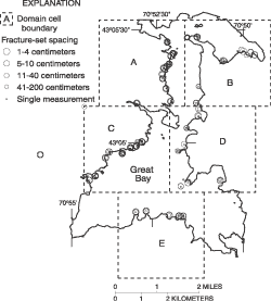
| Figure 2. Location of domain cells and the distribution of fracture-set spacing in relation to the shoreline of Great Bay, N.H. |
The Great Bay area was divided into five regions, or domain cells, of equal size. These domain cells are square regions (3,300 m on a side) drawn in such a way as to contain a nearly equal distribution of outcrops (fig. 2). Two techniques of domain analysis were used. Discrete-measurement analysis gives an equal weight to each fracture orientation at an outcrop. The second technique, spacing-normalized analysis, multiplies a fracture-set observation by a spacing factor, if an outcrop has regularly spaced parallel fractures. This technique gives fracture-set orientation more representation in the analysis.
Both techniques described in the previous paragraph are based on the statistical identification of fracture families. Fracture families (principal trends of fractures) were defined for each domain by plotting normalized azimuth-frequency (rose) diagrams using software (DAISY) by Salvini (2000). A Gaussian curve-fitting routine is used in DAISY for determining peaks in directional data (Salvini and others, 1999) that first was described for lineament analysis by Wise and others (1985). Peaks and the standard deviation for each peak were calculated with DAISY. Peaks with normalized heights greater than 50 percent of the highest peak were considered in this study to be principal trends (Walsh and Clark, 2000). Lineaments in the domain are classified as fracture correlated by domain analysis if their trend is within one standard deviation of a family peak trend (Moore and others, in press).
In discrete-measurement analysis, fracture orientations are weighted equally without considering fracture spacing, or number of fractures at an outcrop. Each fracture orientation measured at any given outcrop is represented as one observation in the analysis. Fractures that are not part of a fracture set are weighted equally in the discrete-measurement analysis. If a given fracture orientation is observed throughout the domain cell, it may contribute to the development of a fracture family because it is observed at numerous outcrops.
Closely spaced fractures potentially may provide a greater number of flow paths for water per unit cross-sectional area of a bedrock aquifer than more widely spaced fractures (Mabee and Hardcastle, 1997). A single measurement of fracture orientation can underrepresent a closely spaced fracture set when plotting rose diagrams that summarize fracture orientations observed in a given region, because a fracture-set orientation represents many fractures. The occurrence of regular and closely spaced fracture sets throughout all five domains (A-E) provides justification for the number of fractures counted using the spacing-normalized analysis (fig. 2).
Spacing-normalized analysis requires a unit cross-sectional length, which is equal to the largest spacing observed among all fracture sets. The unit cross-sectional length divided by the fracture spacing determines fracture frequency. To normalize the number of fractures for spacing, the number of fracture orientations analyzed with DAISY for a given region was multiplied by the calculated fracture frequency. For example, the greatest spacing observed in any fracture set was 2 m. One representative measurement was used for this orientation in the data analysis. In contrast, a fracture measurement from a set with a 20-cm spacing would have 10 orientations included in the spacing-normalized technique.
Next: Bedrock and Fractures
Previous: Introduction
Table of Contents
| AccessibilityFOIAPrivacyPolicies and Notices | |
 |
|