|
||||
| Publications—Open-File Report 2006-1159 |
Velocity, Bathymetry, and Transverse Mixing Characteristics of the Ohio River Upstream from Cincinnati, Ohio, October 2004—March 2006
In cooperation with the Greater Cincinnati Waterworks, Northern Kentucky Water District, and the Awwa Research Foundation
Abstract
Velocity, bathymetry, and transverse (cross-channel) mixing characteristics were studied in a 34-mile study reach of the Ohio River extending from the lower pool of the Captain Anthony Meldahl Lock and Dam, near Willow Grove, Ky, to just downstream from the confluence of the Licking and Ohio Rivers, near Newport, Ky. Information gathered in this study ultimately will be used to parameterize hydrodynamic and water-quality models that are being developed for the study reach.
Velocity data were measured at an average cross-section spacing of about 2,200 feet by means of boat-mounted acoustic Doppler current profilers (ADCPs). ADCP data were postprocessed to create text files describing the three-dimensional velocity characteristics in each transect.
Bathymetry data were measured at an average transect spacing of about 800 feet by means of a boat-mounted single-beam echosounder. Depth information obtained from the echosounder were postprocessed with water-surface slope and elevation information collected during the surveys to compute stream-bed elevations. The bathymetry data were written to text files formatted as a series of space-delimited x-, y-, and z-coordinates.
Two separate dye-tracer studies were done on different days in overlapping stream segments in an 18.3-mile section of the study reach to assess transverse mixing characteristics in the Ohio River. Rhodamine WT dye was injected into the river at a constant rate, and concentrations were measured in downstream cross sections, generally spaced 1 to 2 miles apart. The dye was injected near the Kentucky shoreline during the first study and near the Ohio shoreline during the second study. Dye concentrations were measured along transects in the river by means of calibrated fluorometers equipped with flow-through chambers, automatic temperature compensation, and internal data loggers. The use of flow-through chambers permitted water to be pumped continuously out of the river from selected depths and through the fluorometer for measurement as the boat traversed the river. Time-tagged concentration readings were joined with horizontal coordinate data simultaneously captured from a differentially corrected Global Positioning System (GPS) device to create a plain-text, comma-separated variable file containing spatially tagged dye-concentration data.
Plots showing the transverse variation in relative dye concentration indicate that, within the stream segments sampled, complete transverse mixing of the dye did not occur. In addition, the highest concentrations of dye tended to be nearest the side of the river from which the dye was injected.
Velocity, bathymetry, and dye-concentration data collected during this study are available for Internet download by means of hyperlinks in this report. Data contained in this report were collected between October 2004 and March 2006.
Introduction
The Greater Cincinnati Water Works and the Northern Kentucky Water District provide a total of about 200 Mgal/d of treated water to the Cincinnati metropolitan area and communities in northern Kentucky. A large proportion of the water supplied has its source in the Ohio River.
Contaminants can enter the Ohio River through a variety of routes. Should a harmful contaminant enter the river upstream from water-supply intakes, it is critically important that information be available to assess its mixing and transport characteristics so that the water utilities can take appropriate actions to protect their facilities and their consumers.
The Greater Cincinnati Water Works, Northern Kentucky Water District, and Awwa (American Water Works Association) Research Foundation, along with the U.S. Geological Survey (USGS), cooperated in an effort to characterize the velocity, bathymetry, and transverse mixing characteristics of the Ohio River in a 34 mile study reach extending from the lower pool of the Captain Anthony Meldahl Lock and Dam, near Willow Grove, Ky, to just downstream from the confluence of the Licking River and the Ohio River, near Newport, Ky (fig. 1). The study was conducted between October 2004 and March 2006. Information gathered in this study ultimately will be used to parameterize hydrodynamic and water-quality models that are being developed for the study reach. These models may be used by water-resources managers to help satisfy source-water assessment requirements specified in the 1996 amendments to the Safe Drinking Water Act of 1974 (U.S. Environmental Protection Agency, 1996).
Description of the Study Area
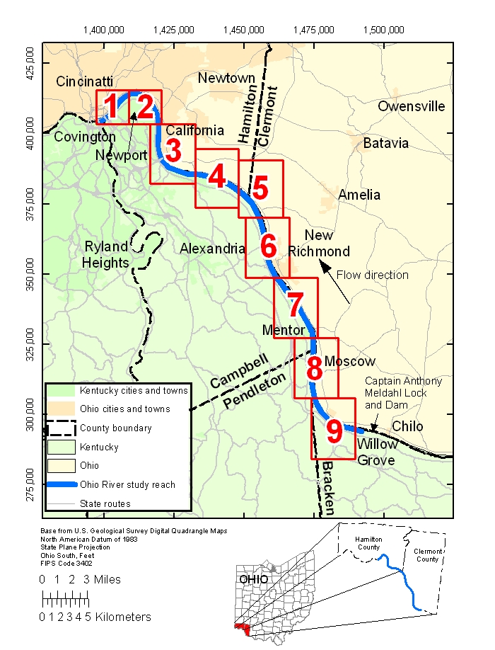
The study area consists of a reach of the Ohio River extending from the lower pool of the Captain Anthony Meldahl Lock and Dam, near Willow Grove, Ky, to just downstream from the confluence of the Licking and Ohio Rivers, near Newport, Ky (fig. 1). The study reach passes through parts of Hamilton and Clermont Counties, Ohio, and parts of Campbell, Pendelton, and Bracken Counties, Ky. The Ohio-Kentucky Stateline follows the Ohio River in the study reach with the Stateline generally located much closer to the Ohio shoreline than to the Kentucky shoreline.
The Ohio River drains an area of about 70,800 mi2 at the upstream end of the reach, increasing to about 76,580 mi2 at the downstream end. Two large streams are tributary to the Ohio River within the study reach. The Licking River, which flows through Kentucky from the south, has a drainage area of about 3,700 mi2. The Little Miami River, which flows through Ohio from the north, has a drainage area of 1,757 mi2. All other tributary streams in the study reach have drainage areas less than 50 mi2.
Water levels in the study reach are controlled in part by the U.S. Army Corps of Engineers' (USACE) operation of the Captain Anthony Meldahl and Markland Locks and Dams. The USACE attempts to maintain a normal pool elevation of about 455 ft (National Geodetic Vertical Datum of 1929). At normal pool elevations, the Ohio River within the study reach ranges in width from about 1,200 to 2,200 ft.
Purpose and Scope
The purpose of this report is to describe the methods and results of a study to determine velocity, bathymetry, and transverse mixing characteristics of the Ohio River in a study reach that extends from the lower pool of the Captain Anthony Meldahl Lock and Dam to just downstream from the confluence of the Licking and Ohio Rivers. Pertinent data gathered for this study are available for download through the Internet by means of hyperlinks contained in this report. Transverse mixing characteristics described in this report may not be representative of characteristics that would be observed for contaminants that are immiscible in water and(or) have specific gravities that are much greater or much less than that of water.
Velocity
Acoustic Doppler Current Profiler (ADCP) Measurements
Boat-mounted broadband acoustic Doppler current profilers (ADCPs) were used to measure velocities and streamflows. The ADCPs used in this study measure velocity by emitting fixed-frequency acoustic signals from four strategically angled transducers and measuring the phase of return signals (echoes) reflected from particles suspended in, and moving with, the water. The phase shift of the reflected signals is used to compute the distance to the suspended particles and to determine the Doppler frequency shift associated with the movement of reflecting particles relative to the ADCP. The return signals are processed (range gated) so that velocities can be determined at a number of depth intervals throughout the water column. The collection of velocities measured by the ADCP over a group of measurement cycles (called pings) is usually averaged to reduce measurement uncertainty and is referred to as an "ensemble". A separate acoustic signal is used to track the river bottom, which permits compensation of velocities for boat movement and determination of the horizontal and vertical components of the water-velocity vectors.
ADCPs measure velocities over most of a typical river cross section; however, small areas near the surface, the bed, and at the edges of the cross section cannot be measured (fig. 2). A small portion of the surface layer is not measured because the transducers must be positioned below the water surface. Another small portion of the surface layer, called the blanking distance, is not measured because residual ringing of the transducers prevents making accurate measurement of near-surface return signals. The blanking distance in this study was 0.25 m (about 0.82 ft). Measurement of velocities near the riverbed (a distance of about 6 to 10 percent of the total depth above the bed) is not possible because the signal reflected from the bed is so strong that it makes it difficult to discriminate between return signals from the main lobe (which travels approximately perpendicular to the transducer face) and side lobes (which travel at angles relative to the main lobe) of the acoustic signal, thereby preventing accurate determination of velocities. Measurement of velocities near the edges of rivers typically is hindered by insufficient depth to overcome measurement limitations associated with transducer ringing and/or side lobe suppression, or due to insufficient physical access. In spite of the inability to directly measure velocities over the entire cross section, extrapolation techniques used when processing the ADCP data have been shown to result in computed streamflows that are within 5 percent of streamflows determined from conventional Price AA-based measurements (Mueller, 2003). For more information on ADCPs and their usage, see http://il.water.usgs.gov/adcp/reports/.
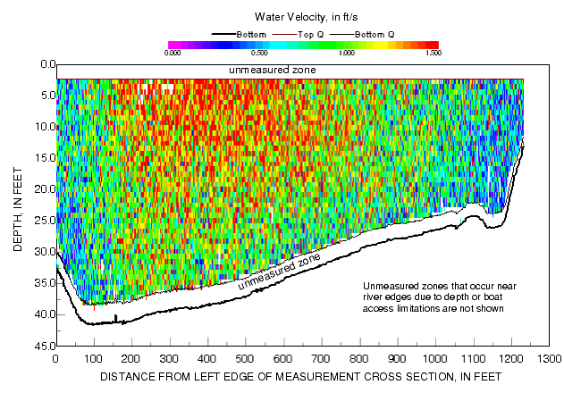
Figure 2. Variation of velocity magnitude between the top (Top Q) and bottom (Bottom Q) of the measured zone along an Ohio River transect. (ft/s, feet per second)
ADCP surveys were done at 80 cross sections in the study reach, and at 2 cross sections on the Little Miami River near its mouth by means of 600-kilohertz (kHz) RD Instruments acoustic Doppler current profilers. The dates and river-mile boundaries of the ADCP surveys are listed in table 1.
The average distance between ADCP cross sections was about 2,200 ft. One transect was done at most cross sections, and at least four transects (two traverses in each direction) were done at cross sections where high-quality streamflow measurements were desired. All transect locations were geolocated by means of onboard differentially corrected Global Positioning System (GPS) units. The locations of all ADCP transect data contained in this report are referenced to the North American Datum of 1983 (NAD 83), Ohio State Plane (Ohio South) coordinates, U.S. Survey Feet.
Postprocessing of ADCP Data
ADCP data were postprocessed to correct errors in position and velocity information and to determine geographic coordinates associated with each ADCP ensemble. Position errors can be due to local anomalies in magnetic north, which are not accounted for in the ADCP configuration files, and to difficulties associated with tracking the streambed from a moving boat by means of acoustic signals. In addition, errors in the distances determined from bottom track measurements can occur if the streambed is moving. Thus, east and north distances indicated by bottom track measurements are not necessarily equal to those that would be obtained with precise GPS measurements.
Differences between GPS and bottom-track-derived coordinates of the first and last ensembles measured in each cross section were used to scale and rotate bottom-track measurements of position and to adjust the azimuths of horizontal velocities. The following paragraphs detail the mathematics of those adjustments originally described by Holtschalg and Koschick (2003). The GPS data are thought to provide a more accurate indication of the absolute position of the profiles than positions based on the bottom-track measurements. The relative positions of the profiles and the horizontal rotation of the velocity vectors, however, are more appropriately based on the bottom-track information. In addition to coordinate adjustments, postprocessing served to reformat the ADCP data to facilitate its subsequent use.
Let Easting1 and EastingN represent the easting coordinates in Ohio State Plane (Ohio South) coordinates (U.S. Survey Feet) derived from GPS coordinates of the beginning and ending ensembles, and let Northing1 and NorthingN be the corresponding northing coordinates. Also, let ΔEasting = EastingN - Easting1 and ΔNorthing = NorthingN - Northing1 be the change in eastings and northings, respectively, as indicated by GPS. Then, the distance between the endpoints of the transect is calculated as
Similarly, for EastBT1 = NorthBT1 = 0 representing the easting and northing of the first ensemble on the transect indicated by the bottom track (BT), and EastBTN and NorthBTN representing the easting and northing of the last ensemble on the transect, the corresponding distance between end points indicated by the BT is
A scale factor, which represents the ratio of the length between the first and last ensembles measured by the GPS and ADCP bottom track respectively, is computed as
This ratio is multiplied by distances indicated by the bottom track to obtain distances consistent with GPS measurements.
The azimuth of the transect, as defined by the endpoints of the transect from GPS measurements is
where the azimuth is the angle computed by the arctangent (atan) function from the specified changes in northing and easting. Here, the results of the arctangent function are positive when measured clockwise from zero degrees north (along the positive y-axis); 2π (360 degrees) was added to negative values of the AzmGPS so that all reported azimuths would be positive. Similarly, the azimuth of the transect defined by BT measurements is
Application of the scale and angle adjustments to positional data is described in the following paragraphs. For each velocity profile indexed by n, for n = 2, 3, . . ., N - 1, the adjusted easting and northing was computed as
where sin and cos are the sine and cosine functions, respectively. The adjusted easting and northing velocity components, VelEastAdj and VelNrthAdj, were computed from the measured velocity magnitudes and azimuths, VelMag and VelAzmMea, as
Bathymetry
Bathymetry data were collected within the study reach between October 2004 and March 2006 by means of a boat-mounted NaviSound 210 single-beam echosounder with an 8-degree transducer and an operating frequency of 190-225 kHz. NaviSound's barcheck calibration utility was used to calculate the correct local speed of sound during calibration of the echosounder. The echosounder was calibrated in shallow water where the speed of sound is expected to be constant with depth.
Transect spacing for the bathymetric survey averaged about 800 ft. Geographic coordinates associated with each depth measurement were determined by means of differentially corrected GPS and referenced to the same coordinate system as the ADCP transects. Postprocessing of the bathymetric survey data was done with the HYPACK hydrographic survey program (HYPACK, Inc., 2006).
Differentially corrected survey-grade GPS units were used in advance of the bathymetric survey to set elevation reference marks along the study reach. The elevation reference marks were used to determine water-surface elevations in the mornings and late afternoons during bathymetric data collection. Water-surface elevation data determined from the elevation reference marks, along with water-surface elevation data measured by means of sensors in the lower pool of the Captain Anthony Meldahl Lock and Dam and at the USGS gaging station in Cincinnati, were used to help define the slope of the water surface. Information on water-surface slope ultimately permitted the determination of streambed elevations from depths.
Geographic coordinates for bathymetry data contained in this report are referenced to the North American Datum of 1983 (NAD 83), Ohio State Plane (Ohio South) coordinates, U.S. Survey Feet. Streambed elevations are reported in feet relative to the North American Vertical Datum of 1988 (NAVD 88).
Transverse Mixing Characteristics
Injection and Measurement of Dye
Rhodamine WT, a red dye that fluoresces when exposed to light in a specific range of wavelengths, was used as a tracer to study mixing characteristics in the Ohio River. Rhodamine WT dye has been used extensively as a tracer in water studies because, at concentrations normally used, (a) it is nontoxic, (b) it is fairly conservative (non-decaying), (c) it fluoresces at a magnitude proportional to its concentration, and (d) it is measurable at very low concentrations (parts per trillion) (Smart and Laidlaw, 1977). The 20 percent aqueous solution of rhodamine WT dye used in this study has a specific gravity of approximately 1.15 at 20ºC, an active ingredient concentration of 230,000 mg/L, and it disperses well in water. As such, rhodamine WT dye is a good analog of a conservative dissolved contaminant.
Rhodamine WT dye was injected at a constant rate by means of a precision piston pump. In advance of the field study, injection rates were determined for a wide range of pump piston-displacement settings by sequentially increasing the piston-displacement setting and, for each setting, measuring the volume of fluid pumped in a fixed amount of time.
Injection of dye was begun more than 18 hours in advance of taking measurements and samples in an attempt to achieve near steady-state dye conditions within each cross section during sampling. True steady-state dye conditions could not be achieved because streamflows were not constant throughout the injection and sampling periods. Dye-injection rates were chosen to obtain a fully mixed dye concentration of about 1 µg/L, based on simple dilution calculations using an estimated average streamflow.
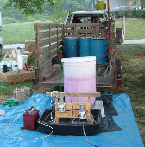
The dye was pumped out of a distribution container (fig. 3) to the river through 3/8-in. inside diameter (ID) polyvinyl chloride (PVC) tubing. A separate pump was used to pump dye from the shipping containers to the distribution container so that there would be no interruption of the injection due to changing dye containers. The discharge end of the injection tubing was held in place in the river at a depth of about 0.5 to 1 ft below the surface by means of a weight and float system.
Fluorescence was measured in the field by means of Turner Designs model 10-AU fluorometers equipped with flowthrough chambers, automatic temperature compensation, and internal data loggers. The use of flowthrough chambers permitted water to be pumped continuously out of the river from selected depths and through the fluorometer for measurement as the boat traversed the river. All traverses were made as nearly perpendicular to the shore as possible. ADCP measurements were made simultaneously during the first traverse in each cross section.
Fluorometers were calibrated according to the manufacturer's instructions on the medium scale with a deionized water blank and a dye standard1 at 10 µg/L. The calibration was checked by analyzing dye standards at 1 and 10 µg/L. A calibration log sheet was completed for each fluorometer on each sampling day.
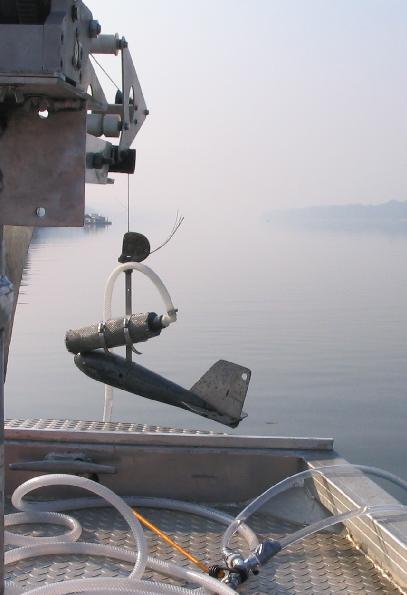
Water was pumped from the river to the fluorometer through translucent 5/8 in. ID reinforced PVC tubing. The ends of the tubing entering and leaving each fluorometer's flowthrough chamber were masked with opaque tape for a length of at least 3 ft to prevent light from being piped into the chamber. The river end of the fluorometer intake tubing was attached to the hanger bar of a crane-suspended streamline weight so that it could be positioned at precise depths below the surface. The intake tubing was screened to prevent clogging of the tubing or pump (fig. 4). An impeller pump, capable of pumping more than 6 gallons per minute, was positioned on the exhaust side of each fluorometer so that water could be drawn through the fluorometer without introducing bubbles into the flowthrough chamber.
Fluorometers were programmed to log time, concentration, and temperature at 10-second intervals and to correct fluorescence readings to a reference temperature of 21°C. Fluorometer clocks were set to Coordinated Universal Time (UTC) at the beginning of each sampling day so that geographic coordinates associated with each data value could be determined by time-matching with GPS data time coordinates that were recorded simultaneously at intervals of 1 second or less. Times associated with fluorometer readings were offset by -30 seconds prior to geographic coordinate lookup to account for the residence time of water in the intake tubing. Residence times were determined by pumping water through the tubing and fluorometer for several minutes and then raising the intake above the water surface and measuring the time required to purge the water contained in the tubing.
The horizontal coordinates of fluorometer and depth measurements collected in association with a given cross section were altered mathematically by projecting the coordinates onto a single vertical plane oriented perpendicular to the river banks. This was done to (a) eliminate horizontal distortion in the transverse direction that would result from a nonlinear ship track or drift of the boats upstream or downstream relative to the ideal cross section, (b) facilitate comparison of concentrations between depths (where multidepth samples were obtained), and (c) to permit visualization of the vertical and transverse variation of dye concentration as a function of cross-section geometry. Projection of the data was necessary because the action of wind, waves, and the river's velocity make it impossible for an untethered boat to traverse the river in a perfectly straight line or to follow identical ship tracks when making multiple traverses.
The projected horizontal coordinates of a given sample were determined by finding the perpendicular to the line representing the ideal cross section (one that is perpendicular to the riverbanks) that passes through the true horizontal coordinates of the sample. The projected horizontal coordinates were set to the coordinates of the intersection of that perpendicular with the line representing the ideal cross section (fig. 5). Horizontal stationing for each sample value was determined by calculating the distance from the starting point of the ideal cross section to the sample value's projected coordinates. The left edge of water (looking downstream) was used as the starting point for each cross section.
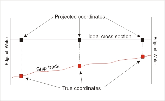
Figure 5. Schematic representation of method used to project ship-track coordinates onto an ideal cross section.
Manual Reference Samples
At least three river-water samples were collected manually per cross section. Samples were collected in clean 30 mL (or larger) glass bottles. Each bottle was filled with water pumped through the fluorometer and then emptied and filled again to obtain the sample. As each bottle was filled, the fluorometer reading and time were read and recorded. Concentrations of dye in manual reference samples were determined later in a laboratory by means of a Turner Designs Model 10 analog fluorometer and then compared to concentrations measured on the river with the flowthrough fluorometers.
Concentrations measured in manual samples may differ from concentrations indicated by the flowthrough fluorometers because the waters on which flowthrough fluorometer measurements are made are, by necessity, different. Because the traveltime from the fluorometer's flowthrough chamber to the discharge point (where manual samples were collected) is short, it is anticipated that differences in concentration will be small, except possibly where the local transverse concentration gradient in the cross section is large.
Testing for Vertically Well Mixed Conditions
Dye concentrations were measured in transects at four depths until vertically well mixed conditions could be reasonably confirmed. Once vertically well mixed conditions were confirmed, dye concentrations were measured at a single depth. Field confirmation of vertically well mixed conditions can be challenging because of difficulty discriminating concentration changes that result from transverse drift of the boat from those that result from true vertical variation. This is particularly true at cross sections where there are large transverse gradients in concentration.
For the purposes of this study, a vertical was considered well mixed if the concentration of dye varied by no more than 5 percent in the vertical. Assessment of vertical mixing was done by dividing the cross section width into four approximately equal-length subsections. Then, beginning approximately at the center of the first subsection closest to the bank from which the dye was injected, the fluorometer intake was lowered to near the bed and then raised back to the surface and the maximum and minimum concentrations observed. If the maximum concentration was less than or equal to 1.05 times the minimum concentration, then that vertical (and subsection) was considered to be well mixed. If the vertical was well mixed in the first subsection, the procedure was repeated in the adjacent subsection. If the second vertical also was well mixed, the entire cross section was considered to be vertically well mixed and subsequent sampling at that cross section was done in a single, approximately mid-depth traverse. All cross sections downstream from that point were also considered to be vertically well mixed. Cross sections were sampled at about 1-mi increments downstream from the first vertically well mixed cross section.
If either the first or the second vertical was not vertically well mixed, the cross section was sampled at four depths. Sample depths were chosen to provide good spatial information on dye concentration both in the vertical and transverse directions. Cross sections were sampled at approximately 2-mi increments until vertically well mixed conditions were observed.
Dye-Tracer Studies
Between August 1 and August 4, 2005, dye and/or ADCP data were collected in an 18.3 mi section of the Ohio River (fig. 6) at a total of 17 cross sections whose positions were determined before the field study. The cross sections are labeled sequentially starting with cross section OH 0 at the upstream end of the dye-study reach (just downstream from the mouth of Big Indian Creek, near river mile 445) and ending with cross section OH 16 at the downstream end of the dye-study reach (downstream from the mouth of Little Miami River, near river mile 464). ADCP data were collected at all 17 cross sections; however, dye data were collected only at cross sections OH 1-16.
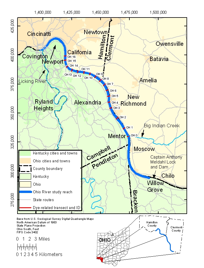
Two separate dye injections were done on different days in overlapping stream segments. The first dye injection on August 1-2, 2005, was used to examine mixing in a downstream stream segment extending from cross section OH 4 to OH 16. The second dye injection on August 3-4, 2005, was used to examine mixing in an upstream stream segment extending from cross section OH 0 to OH 9.
Downstream Study
Starting at 1706 UTC on August 1, 2005, dye was injected about 125 ft off the Kentucky shoreline at cross section OH 4 (approximately 1,180 ft downstream from the mouth of Twelvemile Creek). Dye was injected at a rate of 200 mL/min until 1800 UTC on August 2, 2005. Before beginning fluorometric measurements and sampling on August 2 and August 4, river-water samples were collected upstream from the dye-injection points so that background fluorescence (fluorescence from substances in the water other than dye) could be assessed. Background fluorescence in river-water samples collected on both August 2 and August 4, 2005, measured the equivalent of 0.02 µg/L of dye.
On August 2, 2005, dye and ADCP measurements were started at cross section OH 6 at about 1357 UTC and measurements were made throughout the day ending at cross section OH 16 at about 1854 UTC. Vertically well mixed conditions could not be confirmed at cross sections OH 6 and OH 8, so dye concentrations were measured at four depths. Vertically well mixed conditions were observed at cross section OH 10, so measurements were made at approximately mid-depth at cross sections OH 10-16.
To facilitate comparisons between cross sections, the concentration axis of dye-concentration profiles shown in this report (figs. 7-15 and figs. 18-28) was scaled by dividing each concentration by the maximum concentration observed in that cross section on the day of sampling. The resulting scaled values are referred to as relative concentrations because they are scaled relative to the maximum concentration in the cross section. If more than one traverse was made at a cross section on a given day, then the maximum concentration for all traverses was used to scale the plot. Maximum concentrations used to scale the plots are listed on each plot. Also, a plot of the maximum concentration observed in each cross section on 8/2/2005 as a function of distance from the dye injection point is shown in figure 17.
The dye cloud spread gradually out from the injection (left) bank as it progressed downstream (figs. 7 to 15), possibly reaching the right bank somewhere between cross sections OH 13 and OH 14 (about 9 to 10 mi downstream from the injection point). Each figure shows a plot of the relative dye-concentration profile with an adjacent plot of the cross-section-depth profile (as determined from the ADCP measurement). The appearance of the concentration profile changed appreciably between cross sections OH 13 and OH 14. Whereas concentrations at cross section OH 13 (and upstream cross sections) tended to decrease gradually from the left bank to the right (fig. 12), concentrations at cross section OH 14 were observed to be highest about 700 to 800 ft from the left bank (fig. 13). The reason for the change in appearance is not known with certainty; however, it may be due in part to the influence of Fourmile Creek, which enters the Ohio River from the left (Kentucky) bank, about 0.6 mi upstream from cross section OH 14 (fig. 16). Dye-free water entering the Ohio River from Fourmile Creek, which has a drainage area of about 17.6 mi2, may have diluted dye concentrations in a portion of the cross section or otherwise acted to alter the transverse trend in dye concentration. Because streamflow in Fourmile Creek was decreasing during the period from July 30,2005, to August 5, 2005, any effects that it might have had on the Ohio River should also have decreased over that period. The Little Miami River discharges to the Ohio River between cross sections OH 15 and OH 16. It is probable that the transverse variation in dye concentration at cross section OH 16 also was affected to some degree by the Little Miami River's discharge.
To help assess the relative state of mixing at the cross sections, a coefficient of variation of dye concentrations was computed for each cross section and traverse where vertically mixed conditions were observed (table 2). The coefficient of variation was computed as
If all concentrations measured during a traverse were equal (indicating fully mixed conditions), the coefficient of variation would be zero. As the transverse variation in concentrations becomes more variable, Cv increases. Table 2 shows that Cv decreased monitonically in the downstream direction during the downstream study. Cv values at cross section OH16 were less than one-fifth of that determined for cross section OH 10; however, the standard deviations of concentration values still were greater than 20 percent of the mean concentrations in the traverses. Also shown in table 2 are streamflows, average velocities, and dye concentrations calculated by assuming that the mass rate of dye injected at the injection point is fully mixed in a streamflow equal to that measured at the cross section. The fully-mixed dye concentrations reported in table 2 have not been corrected for changes in concentration that can arise from the effects of longitudinal dispersion or physical and chemical process that can result in loss of dye mass.
section
ID
Velocitya(ft/s)
dye
concentration(%)
bFully mixed dye concentrations were calculated by assuming that the mass rate of dye injected at the injection point is fully mixed in a strreamflow equal to that measured at the cross section. No corrections were made to account for changes in concentration that can arise from the effects of longitudinal dispersion or physical and chemical process that can result in loss of dye mass.
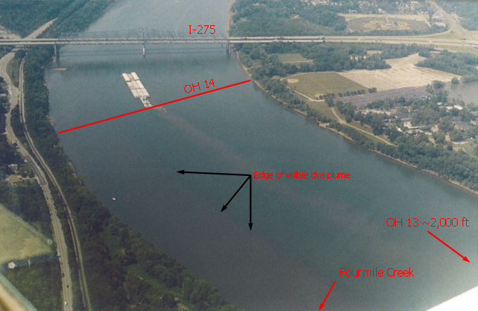
Figure 16. Photograph of the Ohio River near California, Ohio, taken 08/02/05 at approximately 1900 UTC (photograph supplied by the Greater Cincinnati Water Works, reproduced with permission).
On August 2, 2005, traverses were repeated at cross sections OH 15 and OH 16 to assess how concentrations changed over time. Two traverses were made at cross section OH 15 beginning about 48 minutes apart; and at cross section OH 16, three traverses were made, the second traverse beginning about 10 minutes after the first and the third traverse beginning about 43 minutes after the second. The two traverses at cross section OH 15 resulted in very similar concentration patterns over most of the section (fig. 14); however, concentrations near the right bank were appreciably higher on the second traverse. The first two traverses (measured about 10 minutes apart) at cross section OH 16 exhibited concentration patterns that were similar to one another (fig. 15). In both of these traverses, the concentrations tended to be higher along the left (Kentucky) bank than along the right (Ohio) bank. Also, both traverses showed two distinctive depressions (one 500-700 ft from the left bank and the other 900-1,000 ft from the left bank) in their concentration traces. By comparison, the third traverse, measured more than 40 minutes later, still exhibited considerable similarity to the first two traverses with concentrations again higher near the left bank; however, the two depressions observed earlier were less pronounced, and concentrations at distances greater than 1,000 ft from the left bank were only about 65 percent of those observed in the first two traverses.
When the planned dye injection was completed at 1800 UTC on August 2, 2005, the intake side of the injection tubing was removed from the dye distribution container and placed into a container of water, then the pumping rate was increased to purge the volume of dye resident in the injection tubing (about 0.3 ft3). This was done so that the tubing could be stowed for transit to the August 3 injection site without danger of dye spillage. Purging the tubing in that manner did not affect any of the sample results on August 2 because sampling crews were working about 11 mi downstream from the injection point at that time; however, it did cause concern the next day (August 3, 2005) when dye samples collected by a downstream water utility showed an unexpected increase in dye concentration. Although not part of the original sampling plan, the concentration spike associated with purging the dye resident in the injection tubing offered an opportunity to examine mixing characteristics associated with a relatively short-duration pulse of dye yielding higher instream concentrations than from the continuous injection.
USGS crews were working on the river on August 3 to prepare for the second dye injection and the August 4th sampling; however, fluorometers had been removed from the sampling boats at the completion of sampling on August 2 so that they could be checked and recalibrated. Because all other equipment was present on one sampling boat, it was dispatched to the downstream end of the reach where samples were collected manually from cross sections OH 15 and OH 16, along with simultaneous ADCP and GPS measurements. Manual samples on August 3 were collected the same way as manual samples collected on other dates with the exception that the fluorometer that normally would have been in line was replaced by a simple coupling.
The spatial trends in dye concentrations measured on August 3 at cross sections OH 15 and OH 16 were similar to those observed on August 2; however, maximum concentrations at cross sections OH 15 and OH 16 on August 3 were greater than on August 2, presumably in response to the short-duration pulse of dye introduced when the injection tubing was purged. On both August 2 and 3, cross sections OH 15 and OH 16 exhibited concentrations that tended to decrease with distance from the left bank until they reached a local minima near mid-channel, then they increased once again followed by another decrease in concentration near the right bank (figs. 18 and 19). Concentrations were highest near the left bank at cross sections OH 15 and OH 16 on both days.
Upstream Study
Starting at 1836 UTC on August 3, 2005, dye was injected about 60 ft off the Ohio shoreline at cross section OH 0 (about 400 ft downstream from the mouth of Big Indian Creek (fig. 6)). Dye was injected at a rate of 200 mL/min until 1800 UTC on August 4, 2005, when the injection was stopped. Dye and ADCP measurements were started at cross section OH 1 at about 1310 UTC on August 4, 2005, and measurements were made throughout the day, ending at cross section OH 9 at about 1918 UTC.
Vertically well mixed conditions could not be confirmed at cross sections OH 1 and OH 2, so dye concentrations were measured at four depths. Vertically well mixed conditions were observed at cross section OH 3, so measurements were made at approximately mid-depth at cross sections OH 3-9.
The dye cloud spread out from the injection (right) bank as it progressed downstream (figs. 20 to 28), most likely reaching the left bank somewhere between cross sections OH 1 and OH 2 (about 1.5 to 2.5 mi downstream from the injection point). The highest concentration portion of the dye plume appears to have separated from the right bank at cross section OH 4 and remained approximately 300 to 600 ft offshore throughout the remainder of the reach. Concentrations in all cross sections tended to be lower near the left bank than near the right bank, indicating incomplete transverse mixing in the reach. Maximum concentrations used to scale the plots are listed on each plot.
Tests were done at cross section OH 9 on August 4, 2005, to assess the comparability of data collected by the two sampling boats. Both sampling boats traversed the river at the same time, one boat passing about 150 ft upstream from the other. As shown in figure 28, with the exception of a few anomalous readings near the right bank, data collected by the two boats were very similar. A plot of the maximum concentration observed in each cross section on 8/4/2005 as a function of distance from the dye injection point is shown in figure 29.
As was done for the downstream dye study, coefficients of variation of dye concentrations were computed for traverses at each vertically mixed cross section in the upstream dye study (table 2). Table 2 shows that Cv decreased monitonically from cross section OH 3 to cross section OH 7 and then increased some at cross sections OH 8 and OH 9. Cv values at cross section OH 9 were less than one-half of that determined for cross section OH 3; however, the standard deviations of concentration values still were greater than 30 percent of the mean concentrations in the traverses.
Manual Dye Sample Results
All concentration plots derived from fluorometer measurements also show manual-sample results. In general, concentrations determined from manual samples agreed fairly well with observations of concentration readings from the field fluorometers. The average absolute difference between concentrations observed in the field and concentrations measured in the laboratory was 0.12 µg/L.
Hydrology and Streamflow Measurements During the Dye Studies
The hydrology of the study reach is very complex. streamflows are regulated by the Captain Anthony Meldahl Lock and Dam, located about 8.9 mi upstream from cross section OH 0 and by the Markland Lock and Dam located about 67.9 mi downstream from cross section OH 16. In addition to the influence of regulation on mixing characteristics, barges that use the river are another potentially significant source of mixing that is variable and difficult to quantify, further complicating the measurement and interpretation of mixing characteristics.
ADCP streamflow measurements were made during the dye tracer study at the locations listed in table 3. Streamflow measurements were made according to procedures described by Simpson (2001) and according to USGS policy (U.S. Geological Survey, 2002). Although streamflows are computed during single ADCP traverses (as was done in association with transverse measurements of dye), the accuracy and precision of those measurements are unknown due to lack of corroboration by repeated measurements.
study
studySummary information for streamflow measurements made during the dye-tracer studies is shown in table 4. Measured streamflows ranged from 27,800 to 28,600 cfs in the reach sampled on August 2, 2005, and from 20,900 to 21,500 cfs in the reach sampled on August 4, 2005. Daily streamflow data (other than modeled data) have not been collected on the Ohio River near the study area in recent years. However, historical streamflow data for the Ohio River at Cincinnati, Ohio (station number 03255000), collected by the USGS from 1939 to 1975, indicate that streamflows measured during the dye studies were lower than about 55 to 65 percent of the daily mean streamflows that occurred historically during the first four days in August.
The time series of stage data recorded during the dye-tracer studies for the lower pool of the Captain Anthony Meldahl Lock and Dam (data provided by the U.S. Army Corps of Engineers) and at USGS gaging station 03255000, Ohio River at Cincinnati, Ohio, were converted to water-surface elevations (fig. 30). It is apparent from the streamflow data (table 4) and figure 30 that hydraulic conditions were not completely steady during the dye studies.
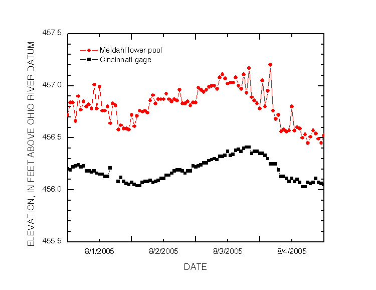
Figure 30. Water-surface elevations at the Captain Anthony Meldahl Dam lower pool and Cincinnati gaging station (03255000) during August 1-4, 2005.
Retrieval of Data
ADCP data that were not collected in association with the dye studies were compiled into seven compressed (zipped) archive files with data grouped by block, as shown in figure 1. The ADCP data are contained in files beginning with the name of the ADCP transect and ending with the extension ".3d." The format of the ADCP files is described in appendix 1. The archive file for each block can be obtained over the Internet by clicking on the appropriate block number from the following list:1, 2, 3, 4, 5, 6, 7, 8, or 9. Once an archive file has been downloaded, individual files contained in the archive can be extracted by means of compression utilities (such as WinZip or 7-zip) that can handle the zip file format.
Bathymetric data collected in 2004-2006 were compiled into a compressed archive file called bathymetry.zip. The bathymetry data are reported as a series of tab-delimited x-, y-, and z-coordinates with x- and y-values in U.S. Survey Feet referenced to the North American Datum (NAD83) of 1983, Ohio State Plane (Ohio South) coordinates, and z-coordinates reported in feet relative to the North American Vertical Datum of 1988 (NAVD 88).
Files containing dye concentration data, cross-section profile data, and associated ADCP data were assembled into a single compressed archive file called dye_data.zip. All dye concentration data measured in the field are in a single comma-separated variable (CSV) file named fluor_data.csv; its format is described in appendix 2. Cross-section profile data are in a single comma-separated variable (CSV) file named xsec_profile.csv whose format is described in appendix 3. Dye concentration data from manual samples are in a single comma-separated variable (CSV) file named manual_sample.csv; its format is described in appendix 4. The ADCP data collected along with the dye data are contained in files that begin with the name of the dye cross section, followed by the date of collection, a boat identifier, a time stamp (only if more than one traverse was made at the transect by a single boat on the same day), and finally with the extension ".3d." The format of the ADCP files is described in appendix 1.
Summary
The U.S. Geological Survey, in cooperation with the Greater Cincinnati Water Works, Northern Kentucky Water District, and the Awwa Research Foundation, collected data to characterize the velocity and bathymetry in a 34 mi reach of the Ohio River extending from the lower pool of the Captain Anthony Meldahl Lock and Dam to just downstream from the confluence of the Licking and Ohio Rivers. Data also were collected to characterize the transverse mixing characteristics of a dye tracer injected into the Ohio River in an 18.5 mi section of that reach. Pertinent data gathered for this study are available for download through the Internet by means of hyperlinks contained in this report.
Two separate dye-tracer studies were done on different days in overlapping stream segments. Rhodamine WT dye was injected into the Ohio River at a constant rate and resulting concentrations were measured in downstream cross sections, generally spaced 1 to 2 mi apart. The dye was injected about 125 ft off the Kentucky shoreline during the first study and about 60 ft off the Ohio shoreline during the second study. Plots showing the transverse variation in relative dye concentration (determined by dividing measured dye concentrations by the maximum concentration observed in the cross section) indicate that, within the stream segments sampled, complete transverse mixing of the dye did not occur. In addition, the highest concentrations of dye tended to be nearest the side of the river from which the dye was injected.
Acknowledgments
The authors thank Mr. Ramesh Kashinkunti, Supervising Engineer with the Greater Cincinnati Water Works, and Messrs. William Yost and David Holtschlag, hydrologists with the USGS, for their assistance and support on this project. In addition, we wish to acknowledge the field and communications support personnel, without whose efforts this study would not have been possible, and the Awwa Research Foundation Project Advisory Committee for their support and insights.
References Cited
Holtschlag, D.J., and Koschik, J.A., 2003, An acoustic Doppler current profiler survey of flow velocities in St. Clair River, a connecting channel of the Great Lakes: U.S. Geological Survey Open-File Report 03-119, accessed September 5, 2005, at http://mi.water.usgs.gov/pubs/OF/OF03-119/index.php
HYPACK, Inc., 2006, HYPACK user's manual: Middletown, Conn, accessed June 6, 2006, at http://www.hypack.com/documentation.asp
Mueller, D.S., 2003, Field evaluation of boat-mounted acoustic Doppler instruments used to measure streamflow: Presented at IEEE Current Measurement Technology Conference, March 2003, accessed April 21, 2006, at http://il.water.usgs.gov/adcp/policy/CMTC_Paper_David_S_Mueller.pdf
Simpson, M., 2001, Discharge measurements using a broad-band acoustic Doppler current profiler: U.S. Geological Survey Open-File Report 01-01, 123 p.
Smart, P.L., and Laidlaw, I.M.S., 1977, An evaluation of some fluorescent dyes for water tracing: Water Resources Research, v. 13, no. 1, p. 15-33.
U.S. Environmental Protection Agency, 1996, 1996 Amendments to the Safe Drinking Water Act - Public Law 104-182: 104th Congress, accessed April 18, 2006, at http://www.epa.gov/safewater/sdwa/text.html
U.S. Geological Survey, 2002, Policy and technical guidance on discharge measurements using acoustic Doppler current profilers: U.S. Geological Survey Technical Memorandum No. 2002.02, accessed September 10, 2005, at http://il.water.usgs.gov/adcp/policy/OSW2002-02.pdf
APPENDIXES
1. Description of data fields in the acoustic Doppler current profiler files
2. Description of data fields in the fluorometric data file
3. Description of data fields in the cross-section profile file
4. Description of data fields in the manual sample file
Appendix 1. Description of data fields in the acoustic Doppler current profiler files.
Appendix 2. Description of the data fields in the fluorometric data file (fluor_data.csv).
Appendix 3. Description of data fields in the cross-section profile file (xsec_profile.csv).
Appendix 4. Description of data fields in the manual sample file (manual_sample.csv)
1Dye standards were prepared by making dilutions with deionized water. Deionized water was used to prepare standards instead of river water because of the potential that background fluorescence and suspended-sediment concentrations in the river could change appreciably between the time that the standards were prepared and the time fluorometric readings were obtained, and therefore would not necessarily result in more accurate dye concentration measurements during the field study.