

StreamStats—A Quarter Century of Delivering Web-Based Geospatial and Hydrologic Information to the Public, and Lessons Learned
Links
- Document: Report (7.67 MB pdf) , HTML , XML
- NGMDB Index Page: National Geologic Map Database Index Page (html)
- Download citation as: RIS | Dublin Core
Acknowledgments
The authors wish to thank the many people who have been involved in the funding and development of StreamStats over the years. This includes all the people from State agencies who have contributed enthusiasm and funding, as well as all of the U.S. Geological Survey (USGS) water science center personnel who have worked to provide data and coordinated with the StreamStats national development team over the years to implement StreamStats for individual States.
Thanks to what was then the Massachusetts Department of Environmental Management (MDEM), now part of the Massachusetts Department of Conservation and Recreation, and to the Massachusetts Department of Environmental Protection (MDEP), for their courage and vision to invest in the initial development of the then-unproven technology that became Massachusetts StreamStats. Thanks, in particular, to Peter Phippen, who led the effort for the MDEM, and to Arthur Screpetis, who led the effort for the MDEP. In addition, thanks to the Massachusetts Bureau of Geographic Information (MassGIS), especially Christian Jacqz, Aleda Freeman, and Philip John, for their contribution of geographic information system data and programming expertise that made Massachusetts StreamStats possible. Also, thanks to Raj Singh, then of Syncline, Inc., for assistance with web programming for Massachusetts StreamStats.
The authors also wish to thank past and present members of the StreamStats national development team for their dedicated work through the years, including Alan Rea, Jacqueline Fahsholtz, David Stewart, John Guthrie, David Litke, Jeremy Newson, Tana Haluska, Ryan Thompson, Katharine Kolb, Martyn Smith, Hans Vraga, Katrin Jacobsen, Tara Gross, Harper Wavra, Andrea Medenblik, Theodore Barnhart, and Timur Sabitov. In addition, thanks to Steven Tessler and Greg Granato for substantial assistance with database design and programming support. Thanks to Mark Bonito, Jonas Casey-Williams, Sara Marcus, and Susan Meacham, all of the USGS, for helping prepare this circular for publication.
The consultants Esri and RESPEC played key roles in the development of StreamStats nationally, and StreamStats would not have been possible without their assistance. In particular, the authors would like to express their appreciation to Dean Djokic, Christine Dartiguenave, and Zichuan Ye, of Esri, and to Paul Hummel, Paul Duda, Robert Dusenberry, and Mark Gray, of RESPEC.
Abstract
StreamStats is a U.S. Geological Survey (USGS) web application that provides streamflow statistics, such as the 1-percent annual exceedance probability peak flow, the mean flow, and the 7-day, 10-year low flow, to the public through a map-based user interface. These statistics are used in many ways, such as in the design of roads, bridges, and other structures; in delineation of floodplains for land-use zoning and setting of insurance rates; for regulatory purposes, such as the permitting of wastewater discharges; and for hydrologic and climate change studies. StreamStats was first developed for Massachusetts and released in 2001. The application provided users with the ability to obtain streamflow statistics computed from data collected at USGS streamgages and to obtain estimates of streamflow statistics for user-selected ungaged sites. Massachusetts StreamStats used geographic information system software and digital mapping to compute drainage-basin characteristics, which were then used in statistical models to estimate streamflow statistics for the user-selected sites. The statistical models were in the form of equations that were developed through a process known as regression analysis. StreamStats was the first known web application with the ability to do interactive geoprocessing.
The utility of Massachusetts StreamStats was instantly apparent, leading the USGS to develop a version of StreamStats that could be implemented nationally. USGS State offices normally were required to develop custom regression equations and prepare local digital mapping data needed for implementing StreamStats for their States. Funding needed to complete this work usually was provided through cooperative agreements between the USGS and State agencies. In 2004, Idaho became the first to be released in the national version of StreamStats. By 2023, 44 States were fully implemented and six were undergoing implementation.
StreamStats has undergone many modifications over the years to keep up with changes to the underlying software and to add functionality. Customized functionality and separate linked StreamStats applications were developed for several States. Meeting the high demand for additions and improvements to StreamStats while also adhering to budgetary constraints has, at times, been challenging. The StreamStats development team has identified numerous additional improvements that could be made to provide better performance and more functionality. The lessons learned from the experience of building and operating StreamStats for nearly 25 years could be relevant to others interested in pursuing efforts of a similar scale.
Introduction
For nearly a quarter century, the StreamStats web application of the U.S. Geological Survey (USGS) has been a source of information used by Federal, State, and local governments, private companies, and others to make decisions about how streamflow may affect the safety and well-being of the public (fig. 1). USGS agency web page usage data indicate that StreamStats is one of the most popular USGS web pages, and as of 2023, the most popular USGS web page used for interactive analyses (fig. 1). The main purpose of StreamStats is to provide estimates of streamflow statistics for user-selected sites on streams, although StreamStats also has several other capabilities for providing information about streams and their drainage basins. Streamflow statistics are indicators of the magnitude, frequency, and duration of streamflow. Some of the most commonly computed statistics are the 1-percent annual exceedance probability peak flow, the mean flow, the median flow, and the 7-day, 10-year low flow. Statistics can be computed from data collected at USGS streamgages or estimated by use of statistical or physical models at locations where data are not available. A complete list of statistics that can be provided by StreamStats for at least some streamgages is provided at https://streamstats.usgs.gov/information-portal/.
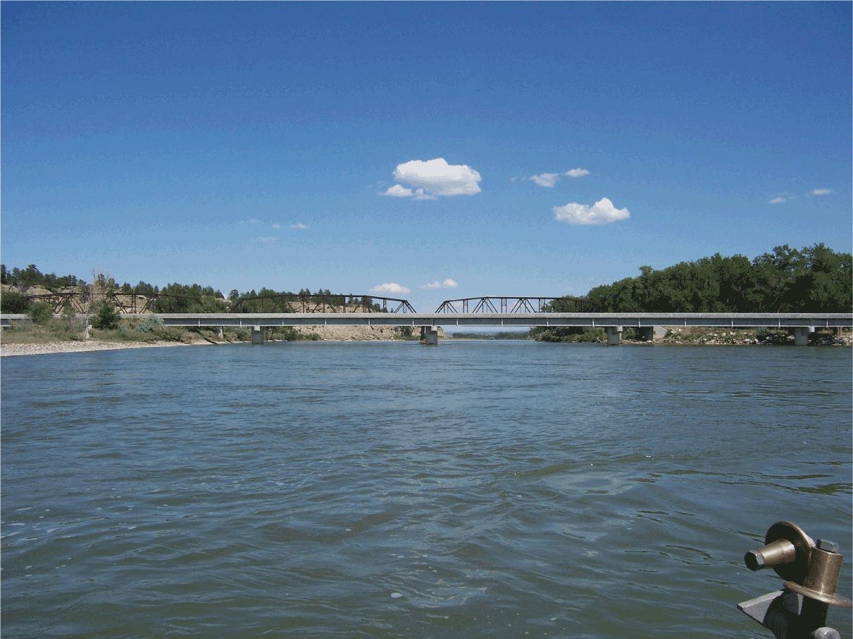
Old (background) and new (foreground) Bundy Road bridges crossing the Yellowstone River near Pompeys Pillar, Montana. Peak streamflow statistics obtained from U.S. Geological Survey statistical models were used to design the new bridge. Photograph by Peter McCarthy, U.S. Geological Survey.
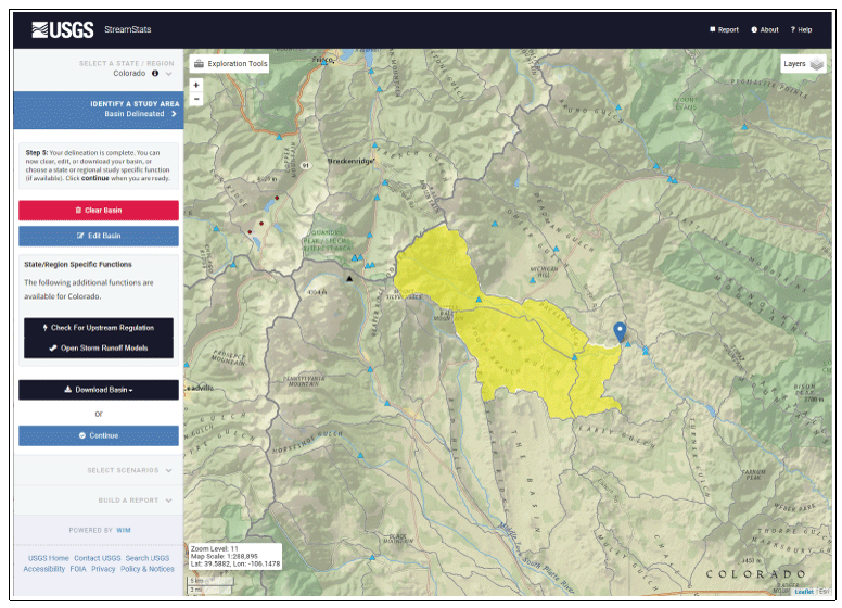
A screen capture of the StreamStats version 4 user interface, with a drainage-basin delineation (in yellow) imposed on a topographic map background. The blue pointer indicates the selected point on the stream for the delineation. Blue triangles are locations of U.S. Geological Survey streamgages for which basin characteristics and streamflow statistics can be obtained. The sidebar to the left allows for selecting an area or a location on which to focus the map initially, such as a town name, and presents a series of buttons that allow users to control the types of information they can obtain.
Streamflow statistics are used by agencies at all levels of government, as well as by private industries, for planning, design, regulation, and permitting of activities in and around rivers and by other users for informational purposes. For example, estimates of the 1-percent annual exceedance probability (equivalent to the 100-year recurrence interval) annual maximum flood are needed for mapping flood-prone areas for land-use zoning, setting insurance rates, and designing bridges, roads, and other structures so that they are not inundated when such events occur. Low-flow statistics, such as the 7-day, 10-year low flow, are used to regulate minimum allowable flows from reservoirs, determine maximum allowable concentrations of contaminants discharged from factories and wastewater-treatment plants, and design culverts with minimum depths needed for fish passage. Statistics, such as the mean and median annual and monthly flows, as well as percentages of time that given flows are exceeded (flow-duration statistics), are used to design and operate reservoirs, water supplies, and industrial facilities.
The USGS began collecting information on the amount of flow in the Nation’s rivers and streams in 1889 (Olson and Norris, 2005). Throughout the years, the USGS has collected at least one full year of continuous streamflow data at more than 24,000 streamgages, more than 10,800 of which are currently active (U.S. Geological Survey, 2022b). The USGS also has collected noncontinuous streamflow data at tens of thousands of other locations. More than 600 types of streamflow statistics have been computed from data collected at these locations and made available to the public through StreamStats.
Streamgage locations represent a very small portion of the possible locations for which there may be a need for streamflow statistics. Consequently, the USGS has used regression analysis to develop equations for estimating streamflow statistics at ungaged sites since at least the early 1960s (Dalrymple, 1960). Development of these equations involves computing the streamflow statistics for a carefully selected group of streamgages and then using a regression analysis that statistically relates the computed streamflow statistics (dependent variables) to physical characteristics of the drainage basins (explanatory variables), such as drainage area, stream slope, and mean basin elevation (Farmer and others, 2019). Estimates of the streamflow statistics for ungaged sites are then calculated by inserting the computed values of the basin characteristics used as explanatory variables into the regression equations.
Regression Equations
The USGS has developed equations to estimate peak-flow frequency statistics for all States, and equations to estimate other types of streamflow statistics for many States. As an example, the equation for estimating the 1-percent probability flood for ungaged sites in hydrologic region 1 of Oklahoma is
whereQ1%
is the estimated peak flow with a 1-percent chance of occurrence in any year and occurs, on average, once in 100 years, in cubic feet per second;
CONTDA
is the contributing drainage area, in square miles; and
PRECIP
is the mean annual precipitation, in inches, as determined by StreamStats.
Lewis, J.M., Hunter, S.L., and Labriola, L.G., 2019, Methods for estimating the magnitude and frequency of peak streamflows for unregulated streams in Oklahoma developed by using streamflow data through 2017: U.S. Geological Survey Scientific Investigations Report 2019–5143, 39 p., accessed March 6, 2023, at https://doi.org/10.3133/sir20195143.
Early applications of regression analysis were mostly for estimating peak-flow statistics for streams, such as the 100-year (1-percent annual exceedance probability) flood (Ries, 2007). These early models were developed before computer technology was generally available, so all of the streamflow statistics and basin characteristics used in these early studies were determined by time-consuming manual processes. By the 1970s, computer technology became available, allowing more efficient computation of the streamflow statistics, but manual methods were still needed to compute the basin characteristics. Determining basin characteristics required precisely drawing (delineating) the basin boundary by hand on topographic maps, computing the drainage area by using a planimeter or digitizing tablet (fig. 2), and then manually transferring the basin boundary to other maps from which the remaining basin characteristics could be computed. The process could take several hours for a basin of a few square miles or several days for a large basin. Also, this process was not entirely reproducible because determining basin boundaries required judgement, and professionals sometimes disagreed about the placement of the boundaries on the topographic maps.
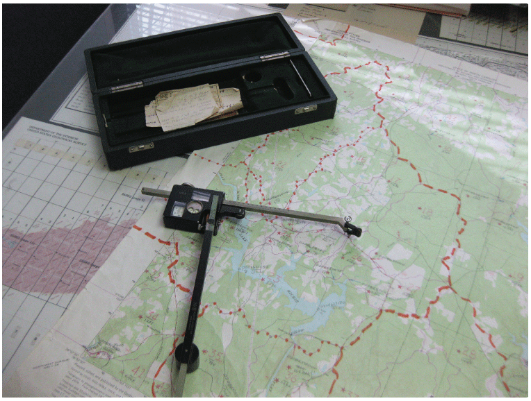
Photograph of a planimeter used to compute drainage areas by following manually drawn drainage boundaries on a topographic map before the advent of geographic information system technology. Photograph courtesy of J. Curtis Weaver, U.S. Geological Survey.
StreamStats automates the processes of delineating drainage basins, computing basin characteristics, and solving the regression equations to obtain estimates of streamflow statistics for ungaged sites. StreamStats users do not need expertise in hydrology or mapping to obtain statistical streamflow estimates, and the results are entirely reproducible. Also, the time required to obtain the estimates is reduced to only a few minutes, which results in substantial cost savings for StreamStats users. For example, the State of Colorado has had StreamStats implemented since 2010. The Colorado Department of Transportation (CDOT) primarily uses StreamStats to estimate peak flows for the design of bridges. CDOT designs hundreds of bridges each year, and in 2016, they estimated a cost savings of $400 per bridge analysis by the use of StreamStats (A. Mommandi, CDOT, written commun., 2016).
StreamStats programmers have used cutting-edge methods to provide information to the public since an initial version, named Massachusetts StreamStats, was developed for the Commonwealth of Massachusetts in 1998. In 2001, demand for this type of information led to the beginning of an effort to develop a new version of StreamStats that could be implemented nationally. Figure 3 presents a timeline of significant StreamStats accomplishments. As of 2023, streamflow statistics are available from StreamStats for streamgages nationally, estimates of streamflow statistics from regression models are available for 44 States and Puerto Rico, and work is ongoing to make regression models available for the six remaining States. Custom functionality for several States also has been developed and implemented. In addition, most of StreamStats functionality is available as web services that can be incorporated into other applications, including a batch process to obtain information automatically for multiple locations.
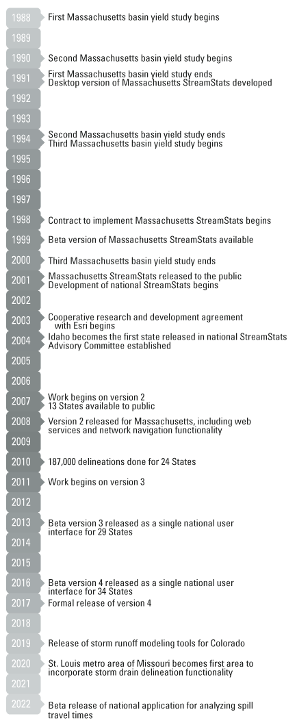
Timeline of significant StreamStats accomplishments.
Continual operation of StreamStats for more than a quarter century, as well as expansion of its geographical and functional capabilities, has required adapting to constant changes in technology, flexibility to accommodate user needs, and close coordination with employees in USGS offices throughout the Nation and with local cooperating agencies. This report describes the initial concept for StreamStats, its development over time, the vision for the future of StreamStats, and lessons learned along the way that may be useful to others interested in pursuing efforts of this scale. The StreamStats home page can be accessed at https://streamstats.usgs.gov, and it provides links to the application, web services, a batch process, and user documentation. Much of the StreamStats programming code is posted at https://code.usgs.gov/StreamStats. This report does not attempt to describe how to use StreamStats. Please refer to the user documentation that can be accessed from the home page for that information.
Initial Concept
The initial concept of Massachusetts StreamStats resulted from a series of three studies, termed “basin yield studies,” done by the USGS in cooperation with what was then the Massachusetts Department of Environmental Management (MDEM), many of the functions of which are now a part of the Massachusetts Department of Conservation and Recreation. The studies provided information that assisted the MDEM in developing water-resource management plans for each of the 27 river basins in Massachusetts (Ries, 1994a, b; Ries and Friesz, 2000). As part of the planning process, the MDEM needed to set minimum streamflow thresholds to meet public demands for water supply while maintaining fisheries and wildlife habitat, recreation, wetlands, and agriculture. The primary aim of the basin yield studies was to develop physically based regional regression models for estimating the 95-, 98-, and 99-percent duration streamflows for locations on Massachusetts streams where no data were available from which to determine the estimates. These low-flow statistics were used by the MDEM as indicators of water availability in the basins.
When the first basin yield study began in 1988, the streamgage data available for developing the regression models were limited, so the accuracy of the resulting models would be less than the MDEM desired. As a result, the first study included establishing a substantial network of streamflow data-collection sites to allow estimation of low-flow statistics at the sites. The second basin yield study then added data collected for the sites from the first study to a new regression analysis to produce more refined models for low-flow statistics. The second study also collected data at additional locations for use in the third and final basin yield study. Ries (1999) described the design and operation of the data-collection network for the basin yield studies and provided the basin characteristics and estimated streamflow statistics for the sites in the network.
In each basin yield study, a group of streamgages were identified in areas with minimally altered flow conditions in and around Massachusetts where data at the streamgages would allow accurate computation of the 95-, 98-, and 99-percent duration streamflows to use as the dependent variables for the regression analyses. Although the regression methods differed among the three basin yield studies (Ries, 1994a, b; Ries and Friesz, 2000), each study required various physical and climate characteristics of the drainage basins (basin characteristics) to be computed for the streamgages. These basin characteristics were tested for use as potential explanatory variables in the regression analyses.
Efforts in the USGS to use geographic information system (GIS) technology to delineate basins and compute individual basin characteristics needed for regression analyses began in the late 1980s. This approach required a skilled GIS specialist and a large investment in GIS software, hardware, and geospatial data, and each basin characteristic for an individual site had to be computed separately. The GIS process was faster and more reproducible than the manual process, but the GIS process was still slow and expensive, and few potential users had the resources to do this kind of processing.
Previous approaches to determining drainage divides from a GIS relied entirely on using an evenly spaced grid (a raster) of elevation points, known as a digital elevation model (DEM). The DEM-based approach involved generating two grids from the DEM data: a flow-direction and a flow-accumulation grid. The flow-direction grid was generated by determining for each grid cell the direction of flow between the cell of interest and the surrounding cell with the largest difference in elevation. For each cell, the flow-accumulation grid was generated by determining the number of cells flowing into it according to the flow-direction grid. Synthetic streams were then created by first setting a minimum threshold value from the flow-accumulation grid as the upstream ends for streams and then following the directions from the flow-direction grid to form the rest of the synthetic stream network downstream (Jenson and Domingue, 1988). The basin area for any specified point on the stream grid could then be determined as the collection of grid cells that flowed to the selected point and had no other cells draining into them. Because of the often-limited accuracy of the available DEMs, a major disadvantage to using this approach was that frequently, the synthetic streams did not agree closely with streams shown on digital versions of topographic maps, and the generated basin boundaries did not agree closely with manual delineations.
At the beginning of the first basin yield study, it was decided that a GIS would be used to determine the basin boundaries and compute the basin characteristics for the streamgages to be used in the regression analyses. For efficiency, computer programming processes were developed to automate this work. The automated basin-delineation process relied on the availability of three principal datasets derived from 1:24,000-scale USGS topographic maps: a raster-based DEM dataset, a digital line graph (DLG) vector-based hydrography dataset, and a vector-based dataset of basin boundaries. The DEM and DLG data were obtained from the USGS Earth Resources Observation and Science (EROS) Data Center for each topographic map with drainage area that drained into Massachusetts. Streams and elevations often did not align between adjacent topographic maps. As a result, it was necessary to process the elevation and hydrography data so that the streams and elevations aligned along the edges of the maps to form seamless datasets. Flow-direction and flow-accumulation grids were then generated from the seamless DEM data. The DLG data required manual editing to align streams that connected across map edges to generate the seamless stream network. The previously delineated basins were constructed by digitizing boundaries for USGS streamgages and other USGS data-collection sites that had been drawn manually on paper topographic maps and rigorously reviewed by trained USGS hydrologists. Previously delineated basins were available for all of Massachusetts, with polygons representing an average drainage-area size of 4 square miles. Digitization and processing into a seamless basin boundary dataset were done in cooperation with MassGIS, the State GIS agency (https://www.mass.gov/orgs/massgis-bureau-of-geographic-information).
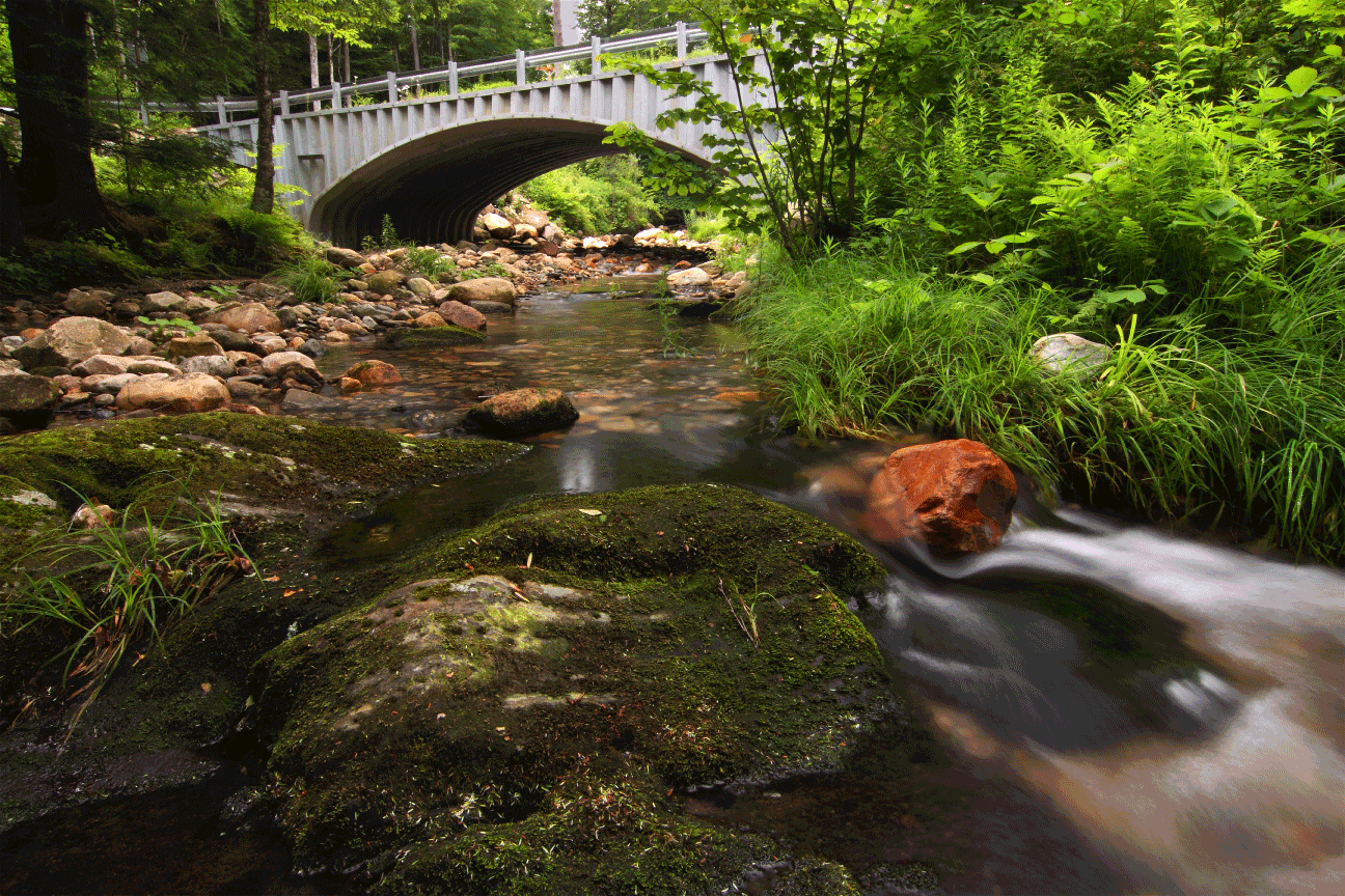
Bronson Brook at Dingle Road in Worthington, Massachusetts, after a stream crossing replacement in 2008. Photograph by Paul Nguyen; used with permission.
The GIS program that was developed for delineating basin boundaries was initially named “ONEBASIN.” In its initial incarnation, ONEBASIN used the vector DLG hydrography as a visual guide to select the location of interest on the raster synthetic stream network for automated basin delineation. The DLG streams were used as the visual guide because those streams were considered more accurate than streams derived from the DEM. Next, ONEBASIN used the DEM raster to derive the drainage divide from the selected point to the intersections with the existing digitized basin-boundary polygons on both sides of the stream. ONEBASIN then accumulated all the upstream polygons of previously delineated basins and dissolved the internal segments of the upstream polygons to produce a single outside boundary for the user-specified site. Figures 4 through 11 provide a visual example of the ONEBASIN delineation process. Subsequent programming steps in the GIS would automatically overlay the basin boundary for a selected streamgage on other digital datasets in a successive manner to calculate the basin characteristics needed for the regression analyses.
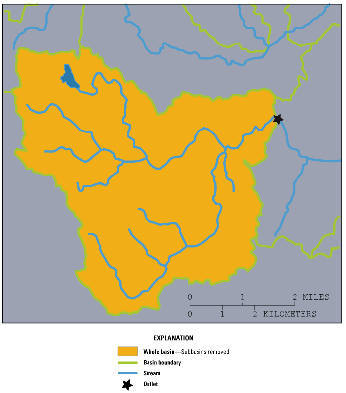
Figures 4 through 11 provide a step-by-step visual example of the ONEBASIN delineation process. Figure 4 is a map of the digital subbasin boundaries and the streamflow network in the Massachusetts part of the Deerfield River Basin, with a user-selected outlet point where a drainage-area delineation is desired. Figure 5 is a screen capture showing a close-up view of selected point on the digital stream network as it appeared originally in the geographic information system program in 1991. Figures 6 through 11 also were taken from 1991 screen captures, but they have been modified for clarity.
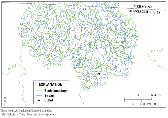
Previously digitized subbasin boundaries and the streamflow network in the Massachusetts part of the Deerfield River Basin, with a user-selected outlet point where a drainage-area delineation is desired.
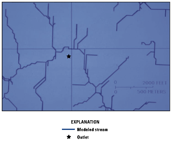
Small scale map of the area around the user-selected point for the basin outlet from figure 4, with blue crosshairs indicating the corresponding point on the digital stream network selected by ONEBASIN.
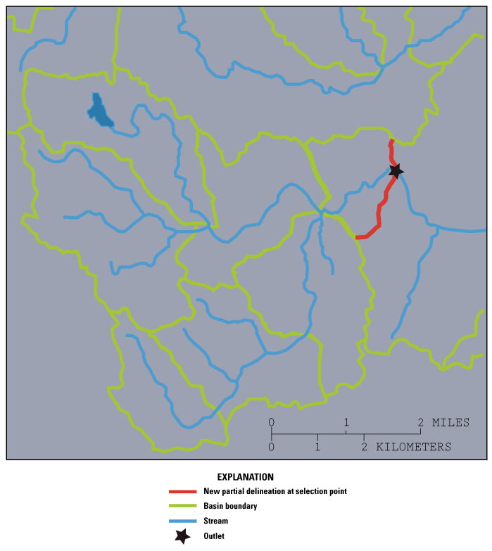
Delineation of the new basin boundary (red) determined from raster elevation data between the selected outlet point and where the new boundary intersects with the existing subbasin boundaries.
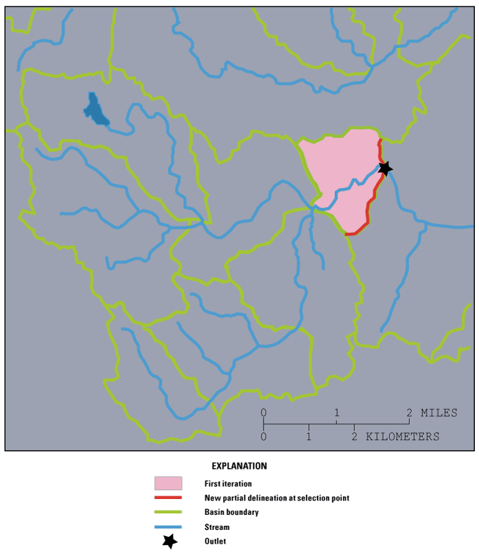
Drainage area (pink) is added between the selected point and the next upstream subbasin.
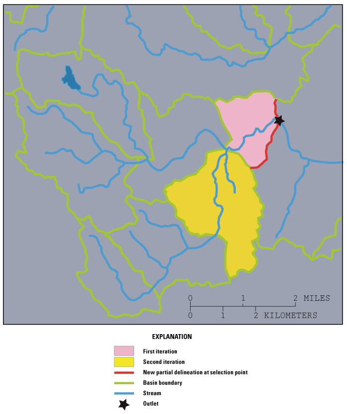
The next upstream subbasin (dark yellow) is captured.
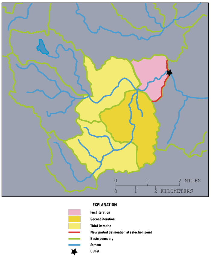
The next two upstream watersheds (light yellow) are captured.
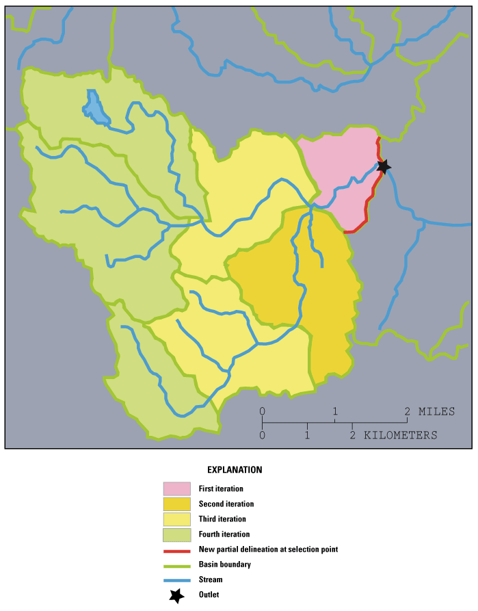
The three most upstream subbasins (light green) are captured.
The internal subbasin boundaries are dissolved to form a single newly delineated watershed (orange).
The initial ONEBASIN approach accomplished many firsts, including the first times that (1) a GIS was automated for use in a USGS regression study, (2) basins were delineated interactively at such an accurate scale, and (3) the more accurate vector hydrography and vector basin boundaries were used as the basis for defining basin boundaries, minimizing the reliance on the less accurate DEM for the delineations. The primary benefit of the ONEBASIN process, in comparison to the purely DEM-based method, was that because the three principal topographic datasets needed for delineations were synchronized, the accuracy of the delineations was substantially improved. An additional benefit of the ONEBASIN approach was speed. The previous, purely DEM-based approach required computations using every grid cell in the raster to determine the basin boundaries, whereas grid-cell computations now were only needed to define the boundary up to the points at which the boundary for a new site intersected with the previously digitized boundaries.
The ONEBASIN process was used in the first basin yield study to determine the basin boundaries and drainage areas for all the streamgages used in the regression analyses to develop equations for estimating the 99-, 98-, and 95-percent duration streamflows. An additional process was developed that would automatically overlay the basin boundary for a selected streamgage from ONEBASIN onto other digital datasets in a successive manner to determine the basin characteristics needed for the regression analyses. After the regression equations became available, this process was modified so it could sequentially run ONEBASIN to delineate the drainage boundary for a specified ungaged site, determine the drainage area and other needed basin characteristics, and then compute the low-flow statistics for the site (Ries and Steeves, 1991).
ONEBASIN also was used to delineate drainage boundaries and compute basin characteristics for the additional streamgages used in the second (Ries, 1994a) and third (Ries and Friesz, 2000) basin yield studies, and then it was modified to incorporate the new regression equations from those studies. The availability of ONEBASIN substantially reduced the cost for computing the basin characteristics needed for the streamgages used in the second and third basin yield studies.
ONEBASIN was improved for the second basin yield study, which began in 1990, first by incorporating an algorithm called ANUDEM (Hutchinson, 1989, 2011) that removes spurious sinks (low points) from the raster DEM and uses the vector hydrography as a guide to modify the elevation data so that the raster streams align more closely with the hydrography. ONEBASIN was also improved by incorporating another algorithm, called AGREE (Hellweger, 1997), which modifies the DEM, in a process known as trenching, to precisely align the DEM with the vector hydrography before deriving the flow-direction and flow-accumulation grids. The AGREE process involves three components that can be adjusted depending on the precision of the data used and the desired result. The first component is the sharp drop distance, which subtracts a large constant negative value from all grid cells that align with the vector hydrography. The second component is a buffer distance, consisting of a number of grid cells from the stream, within which the grid cell elevations will be modified to provide a smooth transition between the original (unmodified) data and the stream. The third component is the smooth drop distance, which is the maximum change in elevation that will be imposed within the transition area. Figure 12 illustrates the characteristic funnel-shaped appearance of a cross section of a modified DEM after the AGREE trenching process was run. This illustration (not drawn to scale) uses a sharp drop of −10,000 meters (m), a buffer width of 60 m (six grid cells), and a smooth drop of −5 m. The component values can be changed depending on the resolution of the available data for a State or region and the desired precision of the derivative data. Running ANUDEM before running AGREE lessens the differences between the raster and vector streams, allowing narrower buffer distances than would be necessary if running AGREE alone and preserving more of the original elevation data (fig. 13). The resulting derivative grids were used only for delineating drainage-basin boundaries, not for computing other basin characteristics.
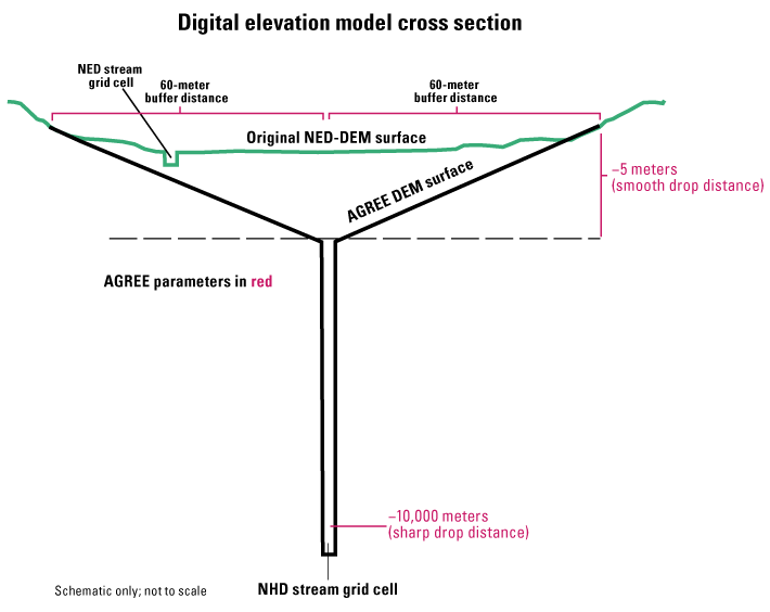
Schematic diagram (not to scale) of a digital elevation model (DEM) cross section showing how the AGREE process makes a stream network derived from a National Elevation Dataset (NED) DEM agree positionally with a stream network taken from the National Hydrography Dataset (NHD). The green line is the original land as defined from the DEM. The solid black line is new surface generated by running the AGREE process with a smooth drop distance of −5 meters depth, a buffer distance of 60 meters horizontally on either side of the grid cell that coincides with the location of the vector stream from the NHD, and a sharp drop distance of −10,000 meters. (Modified from McKay and others, 2012.)
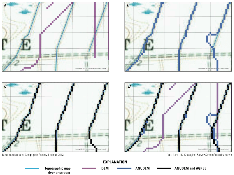
A series of four maps taken from screen captures showing the effects of the ANUDEM and AGREE algorithms included in the ONEBASIN process on the definition of vector streams from raster elevation data. In A, the vector streams derived from a topographic map are shown in light blue imposed on a digital topographic map (blurry because of high magnification), and streams derived from raster digital elevation model (DEM) data are shown in purple. In B, the raster produced by ANUDEM is shown in blue and mostly agrees with the vector stream network. In C, the raster produced by first running ANUDEM and then running AGREE is shown in black, and agreement between the vector and raster streams is exact. In D, the purple grid from the original DEM, the blue grid produced from just the ANUDEM process, and the black grid produced by running ANUDEM and AGREE in sequence are shown together to make it easier to see differences among the grids.
Most DEM data available from the USGS EROS Data Center at the time of the second basin yield study were at 30-m resolution. The DEM data were resampled where necessary across the State and in upstream contributing areas in neighboring States to obtain data with a consistent 10-m resolution. This resampling helped minimize changes to the DEM that were imposed in the AGREE process and helped to better align the DEM with the vector hydrography. Use of a three-cell buffer distance reduced the width of the buffer from 90 m with 30-m grid cells to 30 m with 10-m grid cells, resulting in preservation of more of the original elevation data. The vector hydrography was also improved in additional preprocessing steps by removing braids (sections of stream with multiple channels), resolving discrepancies with the basin boundaries, and connecting disconnected networks through culverts and wetlands. The finished hydrography product resulting from the ANUDEM and AGREE processes, which became known as burning, was a dendritic stream network. The resampling approach used for Massachusetts StreamStats was adopted more than 10 years later by the EROS Data Center in a national program to generate more detailed DEMs for inclusion in the USGS National Elevation Dataset (NED). The approach was also used in the National Hydrography Dataset Watershed Tool (Steeves, 2002).
The programming developed for the basin yield studies in Massachusetts was a major advance in efficiency for delineating basins, obtaining the basin characteristics needed for regression analyses, and creating estimates of flow statistics for ungaged sites. However, obtaining accurate, unbiased estimates of streamflow statistics from regression equations requires use of the same data and methods to compute the basin characteristics for an ungaged site as those that were used to compute the basin characteristics for the streamgages that were used to develop the equations. Although the MDEM had skilled GIS specialists and the GIS software, hardware, and geospatial data that were needed to use the regression equations developed for the basin yield studies, few other potential users did, thus limiting the utility of the regression equations.
The third basin yield study began in 1994. By this time, computer processing speeds and internet technology had advanced to the point where one of the goals of this study was to create a web-based GIS application to provide online users with the ability to obtain estimates of low-flow statistics at ungaged sites and to allow users to get previously published estimates of streamflow statistics for streamgages. The USGS worked closely with MassGIS to accomplish this task. The web application, which was named Massachusetts StreamStats (Ries and others, 2000), consisted of four main components: (1) a user interface that allowed users to navigate on displayed maps, add and subtract map layers, select sites of interest, and display results; (2) a database of previously published streamflow statistics and descriptive information for USGS streamgages in Massachusetts; (3) a database of the GIS data needed to locate sites of interest on the web-based map, compute basin boundaries and basin characteristics, and display additional reference data; and (4) an automated procedure that would delineate the drainage basin boundary for a user-selected site, determine the drainage area and other basin characteristics for the chosen site, and insert them into the regression equations to estimate the streamflow statistics for the site.
The first step in creating the web application was to convert ONEBASIN, originally created by using the ARC Macro Language (AML) programming language of the ARC/INFO GIS software (Esri, 1990, p. 1–2), into an Avenue script (Esri, 1996b) that ran in the program ArcView (Esri, 1996a). The MassGIS office, with guidance from the original ONEBASIN programmer, did most of this conversion, which was necessary because it was not possible to link an AML script to the web at that time. After the conversion, a subroutine was added to insert the computed basin characteristics into the regression equations to estimate the streamflow statistics for a user-selected site and present the results in an output report.
A database of streamflow statistics and descriptive information needed to be created to provide access to information from 725 USGS streamgages in Massachusetts through the web application. This information had been published in 28 separate reports. Many of the reports were out of print, so public access to these data was very limited. Linking of this newly created database to the web application would provide users with a single point of access for streamflow statistics in Massachusetts.
MassGIS provided most of the GIS data for Massachusetts StreamStats. Included in these data were data layers of digital topographic maps, State and town boundaries, streams, and roads needed for detailed site selection; data layers for delineating drainage-basin boundaries and computing the basin characteristics needed to solve the regression equations; and many additional reference data layers. Users could access about 140 different GIS data layers through the user interface. The data layers needed for basin delineations were derived from 1:25,000-scale topographic maps and included networked, centerlined, and reach-coded hydrography; unaltered and drainage-enforced DEMs at 10-m grid spacing; and subbasin boundaries. The hydrography data had a number (reach code) and a direction of flow assigned to each stream segment between confluences (reaches). In addition, lines were added through the centers of wetlands and waterbodies and connected to the stream reaches to form a continuous stream network.
The user interface for the application was developed by Syncline, Inc. (no longer in operation), of Cambridge, Massachusetts, under contract to the USGS. The user interface was built as a Java applet, and a custom connector was built to the ArcView Internet Map Server (ArcIMS; Esri, 1997) software extension to ArcView (Esri, 1996a) to deliver interactive maps to users.
Massachusetts StreamStats was first made available to the MDEM as an internal-only web application in 1998. After thorough testing and publication of the associated reports (Ries and Friesz, 2000; Ries and others, 2000), Massachusetts StreamStats was made available to the public in 2000. This was the first application that allowed for GIS processing over the web in real time; all previous web-based GIS applications served only static information.
In the late 1990s, USGS scientists in New Hampshire (Johnston and others, 2009) developed a desktop process similar to ONEBASIN, called the New England SPARROW (Spatially Referenced Regressions on Watershed Attributes) Method. The chief difference between the two methods was that the New England SPARROW Method used a preprocessing step that formed so-called “walls” in the DEM where it coincided with the previously defined vector basin boundaries. Delineations for new sites were then created by using fully raster-based processing, whereas ONEBASIN used the vector boundaries to the extent possible. A slight compromise in delineation accuracy was accepted with the New England SPARROW Method for the sake of speed, particularly for relatively large basins. This process was used with medium-resolution data (1:100,000/30-m resolution DEM) for development of the New England SPARROW model (Moore and others, 2004). The walling enhancement was adopted for use by StreamStats, with adjustments made for compatibility with the 1:24,000/10-m resolution data being used by StreamStats at the time. The unified approach of burning and walling became known as the New England Method. As of 2022, the New England Method remains the approach used for regional and national USGS programs such as StreamStats, SPARROW, and the National Hydrography Dataset Plus (NHDPlus) (U.S. Environmental Protection Agency, 2020). Although it is preferable to use digital data from the same source scale with this approach, it is possible to use data from differing scales.
Going National
“Streamstats is mission critical for us, we could not function without it at this point.”
—David Knipe, Indiana Department of Natural Resources
Word about Massachusetts StreamStats spread quickly. The principal developers were soon contacted by numerous people within and outside of the USGS who wanted to know how Massachusetts StreamStats worked and how they could get a similar web-based application built for their State. Project personnel also were invited to give presentations to many groups interested in StreamStats, including a presentation at USGS headquarters to senior USGS management.
In 1999, the project chief was tasked with the responsibility for developing a national version of StreamStats that could be implemented for any State. Initial funding for the effort was provided in 2001, and a development team was established to begin implementing StreamStats nationally. The team initially consisted of a hydrologist, two GIS specialists, and an information technology specialist, all of whom worked only part time on StreamStats. The makeup of the team has changed over the years, but it has always included a combination of hydrologists, GIS specialists, computer programmers, and information technology specialists to provide the range of expertise needed for StreamStats to be successful.
Initial Approach to the National Application
In determining an initial approach to building a national application, five considerations were apparent from the start:
-
1. USGS funding would be insufficient to pay for implementing and maintaining StreamStats for all States;
-
2. the ArcView/ArcViewIMS approach that was used for Massachusetts was not scalable, so a new approach was needed for national implementation;
-
3. flexibility was needed for the sources and scales of data used for delineating basin boundaries and computing basin characteristics because data availability varied substantially among individual States;
-
4. the USGS did not have the in-house programming expertise to build a national version of StreamStats, so outside assistance was needed; and
-
5. the national development team was too small to assemble all the geospatial data for implementation of each State, so personnel in the USGS State offices or elsewhere would need to be trained to provide GIS data-preparation assistance.
The USGS operates offices in most States, and the State offices (or the regional centers encompassing those offices) often form cooperative agreements with other Federal, State, and local agencies to share costs for USGS scientists to perform work of mutual interest. In these cooperative agreements, the USGS can provide no more than half of the cost for the work, and often the USGS contribution to costs is substantially less. From the start of the national StreamStats effort, it was determined that federally allocated funding would be used to support the national development team and that USGS State offices would need to form cooperative agreements with other agencies to fund the work needed to implement StreamStats for individual States. Cooperative funding would allow USGS scientists in the State offices to prepare the large GIS datasets required for implementing StreamStats and to work with the national development team on implementation. This approach lessened the cost to the USGS, assured the interest of the State cooperating agencies, and allowed for innovative customization to meet the unique needs of a cooperator. A drawback with the State-based shared-cost approach is that work to implement StreamStats for a given State generally could not begin until a cooperator could be found to help pay for the cost of implementation (as of 2023, only one State did not have a StreamStats application or a cooperator agreement in place with a water science center to develop an application). Another drawback with the State-based approach is that water does not recognize State boundaries. Implementation of StreamStats using a watershed-based approach would have made more sense hydrologically, but taking that approach would have required the difficult task of getting agencies from multiple States to cooperate in order to implement StreamStats for a watershed. Also, existing regression equations for estimating streamflow statistics were almost all developed on a statewide basis, so implementing StreamStats on a watershed basis would have required resolving how to provide estimates for user-selected sites when the drainage areas for those sites fell within multiple States or developing new watershed-based regression equations.
The national version of StreamStats was designed to have a single user interface (front end), with each State set up as a separate application running in the background (back end). This approach eliminated the need to design a separate front end for each State and allowed users to have a single point of access nationally. A watershed approach was used in a few cases where there were specific needs for such an application, as described in the “River Basin Applications and Custom Functionality” section.
Source Data for Delineations and Computing Basin Characteristics
Delineations of basins in StreamStats rely on the horizontal synchronicity of three source datasets: a DEM grid, a vector stream network, and a vector watershed boundary dataset. The accuracy of the basin delineations is highly dependent on the resolution and precision of these datasets, which generally have steadily increased over time (fig. 14). Over the years, the StreamStats development team has coordinated closely with the teams that developed the national core datasets described in the following paragraphs to assure that the timing of data delivery and the structure and quality of the data meet the needs of StreamStats and other interested parties.
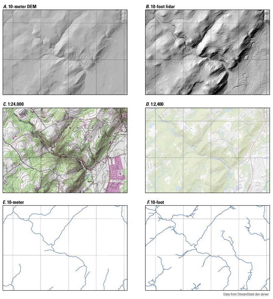
Maps showing the value of higher resolution elevation and stream network data for use in StreamStats. Top left (A) is a portion of the land surface taken from a 10-meter digital elevation model (DEM). Top right (B) is the same area from a 10-foot light detection and ranging (lidar)-derived DEM. The middle left (C) and right (D) are the corresponding 1:24,000-scale and 1:2,400-scale topographic maps for the area. The bottom left (E) and right (F) are the stream networks for the same area, derived from the 10-meter and 10-foot DEMs, respectively. In each case, there is much more detail in the figures on the right than on the left.
Elevation data.—The NED was available nationally at the start of the national StreamStats effort at a 30-m grid-cell spacing, with some areas available at a higher resolution. Most States initially were implemented by using the 30-m data from the NED. For many of these States, the 30-m NED data were resampled to 10-m resolution during the data preparation process. A few States were implemented by using locally available data at a resolution that was higher than the NED.
The elevation data currently used to implement and update StreamStats generally are taken from the USGS 3D Elevation Program (3DEP; U.S. Geological Survey, 2020a), which is the successor to the NED. The scales and sources of elevation data available from the 3DEP vary geographically. Much of the data now available from 3DEP were derived from light detection and ranging (lidar) and are much more precise than the older data from the NED. StreamStats now uses data at 10-m resolution for most implementations. Beginning with North Carolina in 2007, some States have chosen to implement or update StreamStats using higher resolution data, and that trend is expected to continue. StreamStats for 17 counties in western North Carolina was implemented using stream vector data at 1:4,800 scale and DEM data at 20-foot scale generated from lidar (Weaver and others, 2012). Since then, the St. Louis area in Missouri (Southard and others, 2020) was implemented and updates to South Carolina (Feaster and others, 2018) and New Jersey (Watson, 2022) were done using high resolution lidar-based data. The lidar-derived elevation data provide improved accuracy of delineations in relatively flat terrain and for small basins and allow for the potential development of tools for determining channel properties and providing base-level engineering mapping.
Hydrography.— The National Hydrography Dataset (NHD) provides a seamless digital representation of the surface water of the United States (Simley, 2018; U.S. Geological Survey, 2020b). This dataset contains a vector stream network that allows a user to digitally navigate to track water upstream or downstream from any point on the network, a process that is also referred to as tracing. The NHD also allows linking of features such as rivers, streams, water bodies, canals, streamgages, dams, water withdrawals, and point discharges as “events” on the network, with associated attributes. The combination of user-tracing capability and linked events in the database helps with the analysis of cause-and-effect relations, such as whether (and how far) a streamgage is upstream or downstream from a dam that affects the flow of water in a stream, or whether there are any industrial or municipal wastewater discharges upstream from a water-supply intake. This user-tracing capability also allows tracking of an actual or potential contaminant spill through the stream network to help users understand the timing of the movement of the spill and what downstream activities may be affected by it.
The NHD is available nationally as medium-resolution and high-resolution products. The medium-resolution NHD was available at 1:100,000 scale when the national StreamStats effort began. This dataset was developed through a collaboration between the USGS and the U.S. Environmental Protection Agency (EPA) beginning in the late 1990s. A high-resolution, 1:24,000-scale version of the NHD, built in cooperation with the USGS, EPA, and many additional Federal, State, and local agencies, was released nationally in 2007 and, since then, has been the primary hydrography dataset used by StreamStats. The high-resolution NHD is essentially a compilation and sophistication of the original DLG. More recently, NHD with scales of at least 1:5,000 (termed “local-scale NHD”) has been or is being developed in many areas, and some of these local-scale data have been used to implement or update StreamStats.
A large part of the effort needed to implement StreamStats for a State involves quality assurance, editing, and cleanup of the NHD. This work includes making sure that NHD stream reaches have flow directions pointing in the correct direction, removing isolated streams that are not part of the network, and removing braids and canals to create a dendritic network so that flow through the network is confined to a single path (fig. 15). In addition, streamlines are broken at locations of headwater wetlands with multiple streams flowing out of them so that flow from the wetlands would be in only one direction. The final, cleaned-up version of the NHD resulting from this process generally was used in the burning process of the New England Method to generate elevation datasets that were synchronized with the NHD.
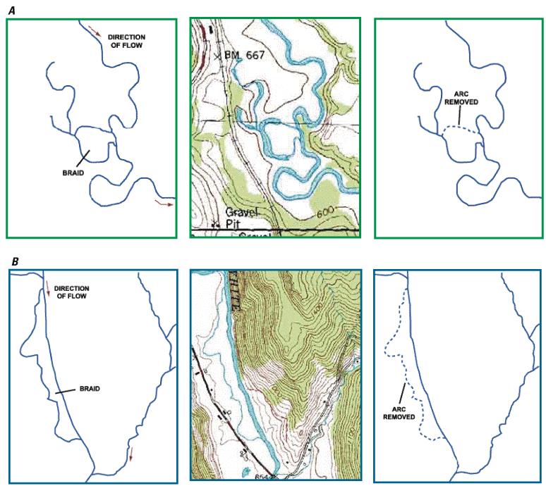
Two diagrams showing examples of editing the National Hydrography Dataset streamlines to remove braids, resulting in a dendritic stream network. On the top (A) and bottom (B) left are sections of streamlines showing the direction of flow and a braid. In the center are topographic maps for the same areas, on which the major streams are shown as double blue lines with blue shading in between, and smaller streams are shown as single blue lines. On the right, the dashed lines indicate where sections were removed to form the dendritic stream networks.
Watershed boundaries.—A nationally available digital dataset of watershed boundaries also was not available at an appropriate scale when the national StreamStats effort began. For States whose applications were implemented early, a digital dataset of previously delineated basin boundaries, usually based on streamgage locations, was provided by the local USGS offices or their partner State agencies, then used in the New England Method walling process to prepare the StreamStats data.
The Watershed Boundary Dataset (WBD) is a hierarchical system of watershed boundaries that were mapped based on surface features at a scale of 1:24,000, by using nationally consistent standards (U.S. Geological Survey and U.S. Department of Agriculture, Natural Resources Conservation Service, 2013), except a scale of 1:25,000 was used in the Caribbean and much of Massachusetts and a scale of 1:63,360 was used in Alaska. The WBD was developed by the National Resources Conservation Service (NRCS) of the U.S. Department of Agriculture and by the USGS, under the coordination of the Advisory Committee on Water Information’s Subcommittee on Spatial Water Data. The WBD divides the Nation into 22 regions that are each assigned a name and 2-digit code. Within each region are as many as seven additional nested levels of subdivision, each with its own assigned name and 2-digit code. Drainage-area sizes at a particular level within the hierarchy vary according to the dictates of the hydrology. The WBD is complete nationally at the 12-digit, subwatershed level. The subwatersheds typically range in drainage-area size from about 15 to 60 square miles (mi2), with an average area of 36 mi2.
The WBD began to be available for individual States in the early 2000s and was typically used in the walling process for StreamStats for States where it was available at the time of implementation. The WBD included basin boundaries for most streamgages with long-term continuous data, but it often did not include basin boundaries for streamgages with shorter records. Consequently, the WBD boundaries were sometimes augmented with boundaries for short-term streamgages that were developed by the individual USGS State offices.
NHDPlus.—The NHDPlus is a set of integrated vector and raster geospatial datasets that provide a national model of how water flows across the landscape. NHDPlus was developed by the EPA, with assistance from the USGS. NHDPlus integrates snapshots (copies of datasets taken at a specific point in time) of the 1 arc-second (approximately 30 m) NED, 1:100,000-scale NHD, and the 1:24,000-scale WBD, and it includes several derivative datasets and value-added attributes that help with hydrologic analysis (U.S. Environmental Protection Agency, 2020). The NHDPlus dataset provides all the data (hydrography, elevation, watershed boundaries, and derivatives) needed to implement drainage-basin delineations in StreamStats. NHDPlus Version 1 was released in 2006 and used to implement StreamStats for California, Idaho, Oregon, Washington, and Wisconsin (Idaho was updated in 2009 using high-resolution data). NHDPlus version 2 was released in 2012 and included substantial improvements over version 1, including improved base datasets, improved processing procedures, and additional attributes. Version 2 was used to implement StreamStats for Kentucky, Montana, and South Carolina.
In 2016, the USGS began an effort to develop a new, high-resolution version of NHDPlus, named NHDPlus HR, and released an initial version in 2022 (U.S. Geological Survey, 2023a). NHDPlus HR was built by using 1/3 arc-second (10-m ground spacing) elevation data from the 3DEP program, along with 1:24,000-scale or better NHD data and 1:24,000-scale WBD data, and it includes many new attributes to provide enhanced functionality. The StreamStats application for Maine was implemented in 2015 using an initial version of NHDPlus HR data and has been the only State to use this dataset. The Maine application was updated in 2023 to use watershed boundaries derived from high-resolution lidar DEMs.
Basin characteristics.—Approximately 275 unique basin characteristics appear in USGS regression equations. The basin characteristics and the source data used to compute them vary widely among the States for which StreamStats has been implemented. Typically, the basin characteristics—such as drainage area, stream slope, and mean basin elevation—that can be computed for a State include all of those used as explanatory variables in the regression equations developed for the State; often, other basin characteristics can be computed, adding value to the application and extending the usefulness to many other scientific or management questions. StreamStats provides a web page at https://streamstats.usgs.gov/information-portal/ that contains links to lists of streamflow statistics, basin characteristics, report citations, and descriptions and metadata of the geospatial data used to implement the application for each State. The individual State pages can be accessed by selecting the State name from that web page.
In 2022, the USGS began implementation of the 3D National Hydrography Program, (3DHP), which is planned to generate new hydrography data for the Nation over 9 years to provide better support for hydrologic modeling and accounting (U.S. Geological Survey, 2023b). The hydrography is being derived from 3DEP DEMs extracted from 1-m lidar, except for Alaska, which is using 5-m DEMs from interferometric synthetic aperture radar. The 3DHP inherits key attributes of the NHD, WBD, and NHDPlus HR and is much more closely integrated with topography derived from 3DEP than those legacy datasets, which the 3DHP will replace. It is anticipated that the new 3DHP data will be used in StreamStats as they become available.
Database Programming Assistance
When Massachusetts StreamStats was implemented, the regression equations used for estimating the streamflow statistics produced by the application were hard coded within the computer programming. A new, national StreamStats application would require a database of the information needed to solve the regression equations for estimating streamflow statistics for each State. Also, the database that held all the previously published statistics for streamgages in Massachusetts would need to be modified and expanded to hold similar information for streamgages nationally.
In 1994, the USGS began distributing a desktop program, named the National Flood Frequency (NFF) program, that solved regression equations for estimating peak-streamflow statistics for ungaged sites. NFF users needed to download and install the program and an associated database before running the program. NFF users would then need to specify (1) a State, (2) a region within the State, and (3) the values of the basin characteristics used as explanatory variables in the regression equations to receive estimates of the streamflow statistics for a site of interest. The NFF program was modified in 2004 to allow estimating other types of streamflow statistics besides those for peak flow, and it was renamed the National Streamflow Statistics (NSS) program (Ries, 2007; U.S. Geological Survey 2019). The NSS program does not include a means for determining the values of the basin characteristics for a site, so users need to determine them by other means. The national StreamStats application took this NSS functionality and incorporated it into a map-based user interface to fully automate the process of selecting a site, computing the basin characteristics, and solving the regression equations.
The NSS program was written in Microsoft Visual Basic, and the database was developed in Microsoft Access by Aqua Terra (now a part of RESPEC) under contract to the USGS. Rather than the StreamStats team attempting to develop its own databases, it was decided that it would be more efficient to have the contractor modify the NSS program and database so the NSS program could be run as a background process by StreamStats. Aqua Terra then modified the NSS program so that it could solve all types of regression equations, such as equations for mean flows and low flows—thus the name change from NFF to NSS. Aqua Terra also combined their Access database for solving regression equations with an Access database that contained previously published streamflow statistics for Massachusetts and made further modifications needed for use in the national StreamStats program. As of 2023, this combined database contained the data needed to solve nearly 7,600 regression equations nationally, and about 2.35 million streamflow statistics for nearly 36,500 USGS streamgages.
The NSS program has many additional capabilities besides solving regression equations to obtain estimates of streamflow statistics for sites of interest, such as estimating weighted streamflow statistics for streamgages and ungaged sites and providing flood frequency and flood hydrograph plots (U.S. Geological Survey, 2019). The USGS has developed a web-based version of NSS that is available at https://streamstats.usgs.gov/nss/. The current (2023) web-based version provides only the functionality for estimating streamflow statistics for ungaged sites because functionality for estimating weighted streamflow statistics for streamgages and ungaged sites is undergoing testing.
“StreamStats is the most efficient hydrological method to delineate drainage basins. It delineates drainage basins in 5–10 minutes compared to 3–4 hours; sometimes 8 hours for large basins, [resulting in] estimated cost savings of about $400 per bridge analysis.”
—Amanullah Mommandi, Colorado Department of Transportation, in presentation from 2016 American Water Resources Summer Specialty Conference: GIS and Water Resources IX, July 11, 2016
GIS Programming Assistance
The StreamStats development team initially contracted in 2002 with a consulting firm to help build a new, web-based user interface that could be implemented nationally. However, this initial contracting effort was not successful, and another approach was needed. Thus, the development team entered into a cooperative research and development agreement (CRADA) with Esri (formerly Environmental Systems Research Institute or ESRI) in 2003 to determine a programming approach for the new national application. At about this same time, Esri was working with the University of Texas at Austin to develop the ArcHydro data model and toolset (Esri Water Resources Team, 2014). The ArcHydro toolset is a no-cost add-on to Esri’s ArcMap software and is used to process DEMs, define streams and catchments, delineate watersheds, and perform other hydrologic analyses. The StreamStats team and Esri decided to take advantage of some of the tools that were already built into the ArcHydro toolset, and linking ArcMap to ArcIMS to enable web functionality was more efficient than developing new programming from scratch. The New England Method of basin delineation, which minimized reliance on the raw DEM for basin delineations, was already included in ArcHydro. Adoption of the use of the ArcHydro toolset and ArcIMS for implementing StreamStats minimized the need for command-line programming for data preparation, making it easier and more efficient for the GIS specialists in local USGS offices to participate in the StreamStats implementation process and gain expertise that would be applicable to many other projects. Additionally, the knowledge gained from using ArcIMS through the CRADA with Esri enabled the StreamStats team to provide support for personnel from local USGS offices who were learning the then-emerging technology for web-enabled mapping applications. Under the CRADA, several new tools were added to ArcHydro for use in StreamStats, and those tools eventually were released in the public version of ArcHydro (current and previous versions and documentation are available at https://www.esri.com/en-us/industries/water-resources/arc-hydro).
The needs for increased stability and speed of delineations were major issues that had to be resolved before StreamStats could be made available nationally. The Massachusetts application had to be closely monitored and reset often to remain online. This level of monitoring would not be possible with a national application including many States; thus, stability was a critical need. The delineation speed of the Massachusetts application was acceptable for that State, but implementation for most other States would require processing much larger GIS datasets than those for Massachusetts. As a result, a more efficient means of on-demand processing of the data was needed to deliver results to users in a timely manner. As GIS datasets have gotten more detailed over time, this need for increased processing speed continues to be a challenge.
The Esri ArcHydro team determined an approach for increasing the basin delineation speed that involved splitting the geospatial data for each area to be included in StreamStats (usually States) by 8-digit hydrologic unit codes (HUCs) (U.S. Geological Survey, 2021) that average about 1,540 mi2 nationally. Any delineation that required a drainage area larger than an 8-digit HUC used a two-tiered functionality designed by Esri: the 8-digit HUC that contained the user-selected site of interest was designated the “local” unit, and upstream HUCs were designated “global” units (fig. 16). Processing needed to define the basin boundary within the local unit for the user-selected site was done interactively. Each local HUC has an associated upstream global HUC except for headwaters HUCs. Drainage areas and other basin attributes for the upstream global HUCs were precomputed so that the total drainage area and other basin characteristics for the site could be determined quickly through mathematical operations (such as summing and averaging) on the values from the local and global units.
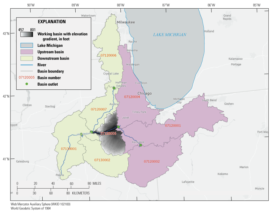
An example of local and global 8-digit hydrologic unit code (HUC) units, where the local HUC in which a point was selected for basin delineation is shown with a gray elevation gradient, the downstream HUCs are shown in green, and the upstream global HUCs are shown in purple. The 8-digit numbers in red are the identifying numbers for the HUCs. Data stored in StreamStats for each local HUC includes all data needed for interactive drainage-area delineation and computation of basin characteristics. Drainage areas and other basin attributes for the upstream global HUCs are precomputed to facilitate quick computations.
Since the earliest days of national implementation, the three base datasets (elevation, hydrography, and basin boundaries) were preprocessed to generate the derivative layers needed for basin delineations. As was done for Massachusetts StreamStats, preprocessing began by imposing the vector streams on the raster elevation data to generate flow-direction and flow-accumulation grids, in which the resulting elevation data were forced to agree with the original vector streams. An optimal threshold number of cells to indicate the upstream end of flowing streams was determined experimentally from the flow-accumulation grid, and the resulting threshold was used to generate a stream-definition grid. From these generated grids, vector stream reach and catchment layers were developed, in which stream reaches generally are lengths of stream between confluences and catchments are the drainage areas that contribute to individual stream reaches. The reach layer was given several attributes to allow determination of properties such as length, slope, and flow direction. The catchments also were given attributes to allow determination of such properties as area and flow direction. This synchronization of the raster and vector datasets for delineations enhanced the capabilities of both datasets, which later led to the development of virtual stream network navigation capabilities for users in StreamStats.
With the geospatial data preprocessed, StreamStats was able to interactively determine the drainage boundary for a new user-selected site within a catchment up to the points at which the new boundary intersected with the existing catchment boundary. StreamStats could then use the catchment attributes to identify any upstream catchments and determine the total basin area for the site. This approach limited the most intensive computer processing to the definition of the new boundary within the initial catchment. However, additional processing of the upstream catchments was still required to determine any needed basin characteristics for the selected site.
The Esri ArcHydro team devised a major innovation by designing an additional derivative-vector layer, called the adjoint catchment layer, that allowed optimization of processing speed within the local HUCs. Preprocessing to generate the adjoint catchment layer used a nesting technique such as the one used to determine global HUCs at the 8-digit HUC level. The adjoint catchment for the catchment of a user-selected site is a single polygon that includes all catchments that are upstream from the initial catchment and has the basin characteristics precomputed as attributes. The addition of this layer substantially reduced the amount of drainage area that needed to be computed on the fly. All six derivative layers (three raster and three vector) work behind the scenes in StreamStats.
Esri also implemented methods to compute a handful of complex basin characteristics, the most important of which was stream slope, which is used in many USGS regression equations. The basin characteristics used in the regression equations varied widely among the States, so the programming needed to compute the characteristics was customized for each implementation of StreamStats by the State offices using ArcHydro XML, an extensible markup language that is customized for use in ArcHydro. More information on ArcHydro, including documentation and installation instructions, can be found at https://www.esri.com/en-us/industries/water-resources/arc-hydro.
The final result of the CRADA with Esri came in January 2005, when the first State, Idaho, was released in national StreamStats, version 1. The new application allowed for a separate map projection for each State and variation of scales in the GIS data used for implementation. These features were important because State cooperators generally wanted to see their States presented in the StreamStats user interface in the projection that they were accustomed to, and the scales of the GIS data needed to implement StreamStats varied widely among the States at that time. The CRADA also resulted in the ability for users to edit basin boundaries and download boundaries, basin characteristics, and flow estimates in shapefiles. Esri also was contracted to assist with resolving many other issues with StreamStats after the initial CRADA expired.
Other Geospatial Considerations
Implementation of StreamStats for each State has required developing map layers for hydrologic regions that correspond to areas within that State where the regression equations for estimating flow statistics for ungaged sites are applicable. Most States have multiple hydrologic regions within the State for a given type of flow statistic, such as peak flows, and many States have regression equations for multiple types of flow statistics, each of which requires a separate map layer of the hydrologic regions for that type of flow statistic. Hydrologic regions within a State usually are defined based on differences in physiography, climate, or both. In most cases, external boundaries of the hydrologic regions correspond with the State borders so that StreamStats users are unable to get estimates of streamflow statistics using the equations for one State when a selected site is outside of that State. In some cases, however, the hydrologic regions extend into adjacent States, such as the Yellowstone River Basin in northwestern Wyoming, where basin delineations, basin characteristics, and flow estimates can be obtained using the Montana application, and the District of Columbia, which has no separate regression equations and has been incorporated into the Maryland application.
Map layers that were termed “hard” and “soft” exclusion zones were set up for many States. When StreamStats was implemented for a particular State, it was necessary to process geospatial data from parts of adjacent States with drainage areas that drained into the State of implementation. Hard exclusion zones were used to disallow delineations for selected sites in the adjacent States when using StreamStats for the State of implementation. Hard exclusion zones also were often established along lengths of major rivers to disallow estimation of flow statistics if the drainage areas for sites along the excluded reaches were much larger than the maximum drainage area for the streamgages used to develop the applicable regression equations, or if flows along those reaches were manipulated to the extent that estimates from regression equations would not reflect actual conditions. Soft exclusion zones were established in some areas where regression equations do not apply, such as southeastern Massachusetts (including Cape Cod), where, because of sandy soils, drainage divides defined by surface topography do not agree with divides determined from mapping of groundwater levels. Users can receive the typical results in soft exclusion zones, but with warning messages.
The approach of using flow-accumulation and flow-direction grids as the basis for determining basin boundaries tended to be inaccurate in flat areas, where elevations in the non-lidar-derived source DEM were nearly all the same. Other types of terrain also presented unique challenges, including along coastlines, in areas with closed drainage and areas with karst topography that formed sinks, in some urban areas, and in inland wetlands and water bodies. Special data-processing steps that had to be taken for these areas are explained in the following paragraphs.
Coastlines.—Delineations of basin boundaries at or near the land/sea interface often were incorrect because of the flat terrain along many coastlines. In most States with this issue, the land/sea interface was addressed by (1) redefining the geographic extent of the local HUC to include an adjacent chunk of offshore area; (2) extracting the coastline features from the NHD and using these features to manipulate the DEM data so that all elevation values on the land side of the coastline with values of 0 or less were assigned a small positive value (in most cases, 1 centimeter) and all sea-side values were assigned 0; and (3) extending the dendritic network out and through the sea portion of the redefined HUC. After these adjustments, the standard ANUDEM and AGREE tools could be used for defining basin boundaries.
Sinks.—Types of terrain that were treated uniformly as sinks included karst areas, prairie potholes (mostly in the upper Midwest), alluvial fans where flows from upstream are absorbed into the sediments, and closed basins in much of the West. Points were manually placed at sink locations during the data preprocessing, rasterized, and assigned a special value in the flow-direction grids. These values were then treated as outlet pour points so that upstream flow would be considered as being from within the sink's watershed. Delineations at a sink point will result in a sink watershed. When it is known where the flow eventually ends up downstream (for example, flow reemerging to the surface through karst or storm drains), these areas can be included in the larger stream network.
Urban storm-drain networks.—Mapped streamlines in urban areas often are discontinuous, with breaks in the streamlines occurring when the streams are diverted into underground channels to become part of the storm-drain network. As a result, drainage-area delineations in urban areas often are erroneous. Recently, the approach described above for sinks was applied to some urban storm-drain networks where the storm drains were treated as sinks, and delineations at storm drain locations captured the drainage areas that contributed to flow into them through open channels and storm-grate catchments. This approach was first applied to the St. Louis metropolitan area of Missouri (Southard and others, 2020), where storm sewer pipes 8 inches or greater in diameter were digitized and connected in a GIS to the storm drains and surface stream networks to help with accurate computation of drainage areas anywhere along the storm sewer and stream networks (fig. 17). This approach of treating storm drains like sinks, which was developed with assistance from Esri, has since been applied to watersheds within Washington, D.C., and in the Mystic River Basin in Massachusetts. High-quality elevation data, such as lidar, and a comprehensive geodatabase of the storm sewer system are needed for this type of processing.
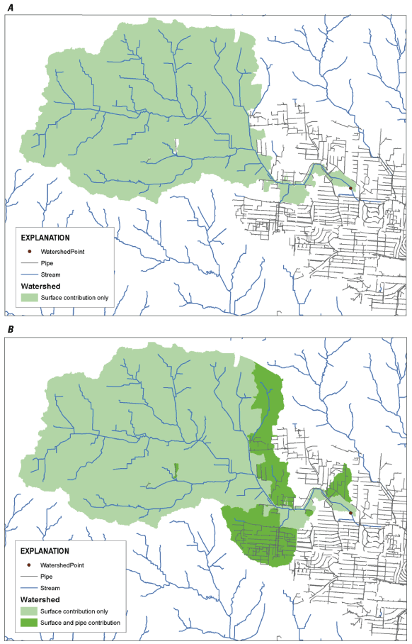
An example of a drainage-area delineation for a point on a storm sewer in St. Louis, Missouri with and without stormwater drainage. In A, the contributing drainage area corresponding to a user-selected watershed point is shown in light green. In B, the contributing drainage area for the same selected point includes contributions from the sewer pipe network, shown in dark green. Gray lines indicate storm sewers and blue lines indicate the surface stream network in both illustrations.
Inland water bodies and wetlands.—Because inland water bodies and wetlands are flat areas on the landscape, a banding effect often can be seen in stream grids generated from the DEM. A bathymetric-gradient process was applied to overcome this banding effect by using the vector stream network to define more realistic stream grids within the water bodies and wetlands. This process creates slopes in the DEM from the edges of the water bodies and wetlands inward toward the elevation grid cells that correspond with the enclosed vector streams (fig. 18). The effect is to create a concave bowl within the water body or wetland, with the stream at the center of the bowl. The process then generates the elevation derivatives from the modified DEM. This process also has the added effect of enforcing delineations at the outlets of water bodies to honor the shoreline rather than cutting though a portion of it.
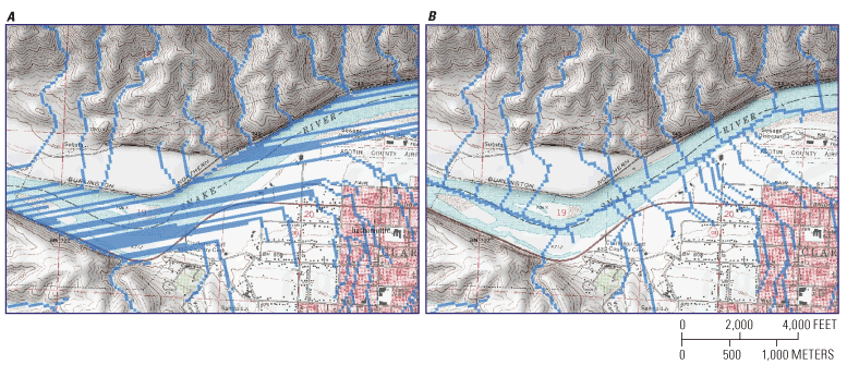
Example of the process used to define the synthetic stream channel through a water body. A is a view of the digital elevation model (DEM)-derived stream grid through a water body, and B is the same location showing the result on the stream grid after the bathymetric gradient process was applied.
Coordination of Activities
The StreamStats development team interacts with scientists in the USGS State offices throughout the process of implementing StreamStats for individual States. This process starts with either the USGS State office approaching State agencies or other potential cooperators about the possibility of cooperating on a project to implement StreamStats, or the USGS being approached by other agencies to implement StreamStats. In either case, scientists from the USGS State offices develop a project proposal describing the purpose and scope of the proposed project, the approach to be taken, the costs, the personnel to work on the project, and the timeline for the work to be done. StreamStats implementation proposals often include the development of new regression equations for estimating streamflow statistics in addition to implementing StreamStats. The project proposal is then presented to the potential cooperating agencies. Projects typically cannot begin until one or more agencies sign an agreement to fund at least half of the cost of the project. In projects that have been completed already, cooperators usually have paid substantially more than half of the cost, with the USGS funding the remainder.
Costs for StreamStats projects have varied widely among the States, depending on the size of the State, which dictates the amount of GIS data to be processed; types and numbers of regression equations to be implemented and basin characteristics used in the equations; whether new equations were developed as part of the project; and whether new functionality or other work was included in the projects. Scientists in State USGS offices are required to consult the StreamStats development team in the process of developing proposals to assure that project costs and proposed timing will be adequate to meet objectives. The StreamStats development team is required to provide reviews of all completed proposals before any agreements can be signed, which also assures that the team is aware of the scope of the work to be done and the timeline for when it is needed.
StreamStats development team GIS experts usually trained GIS specialists in the USGS State offices to generate the geospatial datasets needed to implement StreamStats for their States, including (1) DEM derivative grids, (2) updated and edited NHD streams, (3) datasets needed to compute basin characteristics, (4) hydrologic region boundaries, (5) any special display map layers, (6) streamgage locations, and (7) exclusion areas. Knowledge gained through StreamStats data preparation has often led to other program-development opportunities in the USGS offices. In some cases, a USGS State office did not have a GIS specialist with the needed skills, and the work had to be given to a GIS specialist from another USGS office or a specialist on the national development team. Completion of the data-preparation tasks required very close communication between the State and development team GIS specialists, and, in a few cases, personnel from cooperating agencies and other organizations assisted with the GIS data preparation.
Quality assurance of the basin-boundary and stream-network datasets usually was a large component of the data-preparation process. Typically, a GIS specialist from a USGS State office prepared sample data for a part of the area for which StreamStats was to be implemented and provided it to the development team GIS specialists for review before proceeding with data development for the rest of the area. The State GIS specialists often forwarded corrections to the NHD and WBD data for incorporation into those datasets. A combination of DEMs with 10-m grid spacing, 1:24,000-scale streams, and 1:24,000 basin boundaries was used to develop the derivative grids for most States. Some States used different combinations of data scales, depending on data availability and financial resources at the time of implementation. StreamStats was initially implemented for California, Oregon, Washington, and Idaho by using NHDPlus version 1 data, developed from 30-m DEMs, 1:100,000-scale streams, and 1:24,000-scale basin boundaries (U.S. Environmental Protection Agency, 2020). Idaho was updated in 2009 to use the typical combination of higher resolution data.
After the GIS specialists in State USGS offices delivered their complete data to the national development team, the team would set up a test StreamStats website to enable testing of basin delineations, computation of the basin characteristics, and determining estimates of streamflow statistics for user-selected sites. The locations of a group of streamgages that had been used to develop the regression equations would be submitted in a batch process to the test site. The output from the batch process would be compared to the previously published basin characteristics and flow statistics for the streamgages, and the accuracy of the StreamStats results would be evaluated and documented.
Problems with StreamStats test results were often found during the initial testing. Efforts required to fix the problems varied widely among the States for which StreamStats was implemented. These efforts ranged from fixing a typographic error in a regression equation to having to develop entirely new GIS datasets or regression equations from scratch. In a few cases where the regression equations were developed by using basin characteristics that had not been computed with a GIS, the basin characteristics could not be reproduced adequately, so the equations could not be implemented. After all the obvious problems were eliminated, the cooperating agencies were invited to thoroughly test their individual State applications. Applications were released to the public when the USGS and the cooperating agencies agreed that StreamStats was providing accurate information. The StreamStats development team, scientists from the USGS State offices, and cooperating agencies worked together to write an application information page that is provided for each State in StreamStats.
The StreamStats development team has met regularly for several years with other USGS internal and external entities to coordinate activities and exchange information. Regular meetings are held with the
-
1. USGS 3DHP working group (formerly NHD advisory committee);
-
2. USGS 3DHP technical working group;
-
3. USGS National Geospatial Program (NGP) regional and national liaisons;
-
4. Canadian government and International Joint Commission on transboundary data harmonization;
-
5. WBD dataset technical exchange committee;
-
6. Federal Advisory Committee on Water Information (ACWI), National Hydrography Infrastructure Working Group (currently [2023] not active);
-
7. USGS Lidar User Group;
-
8. Community for Data Integration, Metadata Reviewers Community of Practice;
-
9. USGS Fire Science Community of Practice;
-
10. USGS National Hydrologic Geospatial Fabric (NHGF), NGP, and StreamStats coordination group; and
-
11. ACWI Subcommittee on Spatial Water Data.
River Basin Applications and Custom Functionality
A map showing the status of where StreamStats has been implemented or is undergoing implementation, including the locations of the river basin applications, can be found by clicking on the About button at the top right of the StreamStats user interface. StreamStats applications have been set up for the Connecticut River Basin (in parts of Connecticut, Massachusetts, New Hampshire, and Vermont), Delaware River Basin (in parts of Delaware, Maryland, New Jersey, New York, and Pennsylvania), and the Lake of the Woods–Rainy River Basin (in parts of Minnesota and the Canadian Provinces of Manitoba and Ontario). The river basin applications were set up to address needs that were specific to those areas:
-
• The Connecticut River Basin application was set up to allow basin delineations and computation of basin characteristics needed as input to the Connecticut River Unimpacted Streamflow Estimation (CRUISE) tool. CRUISE is a spreadsheet program that estimates daily streamflow from October 1, 1960, through September 30, 2004, for user-selected ungaged sites on the Connecticut River (Archfield and Steeves, 2012; Archfield and others, 2013).
-
• The Delaware River Basin (DRB) application was set up to delineate drainage areas, to compute the basin characteristics, and to provide water-use summaries that are needed as input for the DRB Streamflow Estimation Tool (DRB–SET; Stuckey and Ulrich, 2016; U.S. Geological Survey, 2016). The DRB-SET tool can estimate daily mean streamflows under baseline (natural flow) and altered (affected by water use) conditions from 1960 to 2010 for user-selected sites on ungaged streams in the DRB. These estimates aid water-resource managers in determining water allocations for maintaining ecological and human-health needs.
-
• The application for the Lake of the Woods–Rainy River Basin, which straddles the boundary between Minnesota and Ontario, Canada, was implemented as part of a larger effort funded by the International Joint Commission (https://www.ijc.org/en) that also included harmonizing hydrography across the United States-Canadian border and developing regression equations for estimating peak-flow statistics at ungaged sites in the basin (Sanocki and others, 2019). This was the first StreamStats application implemented at least partly outside of the United States and helped the development team understand the challenges to be faced if additional international applications were to be considered.
Cooperating agencies for several States requested that custom functionality be included as part of implementing StreamStats. In addition, implementation of StreamStats for a State sometimes spawned separate applications that relied on StreamStats web services for some functionality. Custom functionality developed for some States has occasionally been adopted for use by other States. States with unique functionality include the following:
-
• Colorado and Montana have a “Check for Upstream Regulation” tool that, when used, shades the area(s) within a delineated basin that are regulated by dams in orange and provides the percentage of the total basin area that is regulated. This functionality was first implemented for Colorado and later adopted for Montana.
-
• Colorado’s application also includes functionality for estimating peak storm-event runoff for very small drainage basins in urban areas using the TR–55 model (U.S. Department of Agriculture, Soil Conservation Service, 1986) and the rational method (Dhakal, 2012). These methods are most useful for locations with drainage-area sizes that are near to or less than the lower limit of applicability of 1 square mile of drainage area that is given for the Colorado peak-flow regression equations. This functionality was developed by using a scalable architecture that can help with expansion of this feature to other regions.
-
• Indiana has a StreamStats application that provides flood-frequency estimates for many stream reaches with values that have been coordinated (agreed upon) by the Indiana Department of Natural Resources, the NRCS, the U.S. Army Corps of Engineers, and the USGS for use in water-resources investigations and planning activities. StreamStats users who select points along the coordinated stream reaches will be provided with the coordinated streamflows instead of flow estimates obtained from regression equations.
-
• Maryland has functionality to provide summaries of water use, which was first made available for northeastern Maryland in 2010. Since then, similar water-use functionality has been added to the applications for the Delaware River Basin, Pennsylvania, Connecticut, Massachusetts, and northeastern Ohio. The functionality varies somewhat among the applications depending on local needs and data availability.
-
• Idaho, Oregon, and Washington State have a tool to display Probability of Streamflow Permanence (PROSPER) model outputs developed by the USGS. These PROSPER outputs are in the form of 30-m spatial resolution grids showing colored pixels that indicate the annual (2004–16) probability of a stream channel having year-round flow (streamflow permanence probabilities) and streamflow permanence classes (categorical wet/dry with associated confidence levels) (Jaeger and others, 2019). This information is used for assessments of aquatic and terrestrial species vulnerability and for land and water-quality management.
-
• Missouri has a separate application set up specifically for the metropolitan area of St. Louis that is accessible from the StreamStats user interface (Southard and others, 2020). Drainage-area delineations obtained by using StreamStats for selected sites within this area incorporate drainage through storm drains and thus are more accurate than drainage areas that do not account for storm drains. This functionality was developed by using new tools developed by the Esri ArcHydro Team, lidar-derived DEMs, and locally mapped storm-drain vectors that were processed to enforce drainage through storm drains that are 8 inches and larger in diameter. However, flow estimates from the regression equations should be used with caution because the drainage areas for streamgages used to develop the regression equations did not account for drainage though storm drains (Southard, 2010). Depending on the location selected, a delineation may include only the streamflow network, only the storm-drain network, or a combination of both. Delineated drainage areas for storm drains may appear discontinuous (fig. 17). Regression equations for estimating peak-flow statistics in this area assume that urban land-use characteristics are present (Southard, 2010). Based on the technology developed for metropolitan St. Louis, similar applications were developed for the Mystic River Basin in Massachusetts and for Washington, D.C.
-
• Massachusetts, Connecticut, Pennsylvania, and Iowa have had tools developed that are similar to the separate flow-estimation programs mentioned previously that rely on output from the Connecticut and Delaware River Basin StreamStats applications. The functionality of the programs varies somewhat. Most of them estimate daily-flow time series for a specified period for a selected site and adjust the estimated daily flows for water use. A similar tool for estimating daily time series at ungaged locations has been incorporated into StreamStats for Iowa and can be expanded to other States.
Many other States have also requested the ability to compute unique basin characteristics, or to compute certain basin characteristics that are computed for other States, but in a way that is unique for their State. For brevity, these customizations are not listed above. Information about custom functionality or a separate application for a State can be found, along with links to additional information, by clicking on the About button on the StreamStats user interface after first selecting the State or region of interest.
Advisory Committee
The size and scope of the StreamStats effort required decisions on technical and policy issues that had to be accepted throughout many USGS offices and by the cooperating agencies. As a result, the StreamStats Advisory Committee (SSAC) was formed in 2004 to evaluate these technical and policy issues and to recommend technical approaches, development priorities, and policies needed to successfully implement StreamStats nationally to the development team and USGS management. Initially, the SSAC included 10 members who were selected because of their understanding, interest, and knowledge of statistical hydrology, mapping, and computer applications, and their ability and willingness to communicate with their colleagues. Members typically served staggered 3-year terms, so a third of the SSAC membership changed annually.
The SSAC developed an initial 5-year national implementation plan for StreamStats in 2005 and has updated it several times over the years. The initial plan recommended solutions for several technical issues, such as server and software strategies and approaches to functionality. The SSAC also produced several policy recommendations for implementation USGS-wide, including (1) assessing local USGS offices to recover part of the development team costs to support implementing StreamStats for the States, (2) encouraging development of applications with geographic boundaries that conformed to river basins rather than to State boundaries, (3) standardizing the names of streamflow statistics and basin characteristics across State lines, (4) mandating reviews of proposals produced by the local USGS offices for implementing StreamStats by the StreamStats development team, and (5) handling of multiple values of the same statistics in StreamStats outputs for streamgages. The SSAC also released an internal report in 2013 that provided a comprehensive approach for how StreamStats implementation could be completed for States where State agencies were unable to provide cooperative funding to support implementation costs. The SSAC has been idle since 2017.
“Over the next ten years, South Carolina Department of Transportation (SCDOT) anticipates a savings of $20,300,000 (20.3 million dollars) in engineering costs. Further, the research led SCDOT to modify the Requirement for Hydraulic Design Studies and designated StreamStats as the recommended method for delineating watersheds and obtaining discharges.”
—Abstract submitted to the American Association of State Highway and Transportation Officials, Research Advisory Committee's Value of Research Task Force (written communication to Jimmy Clark, USGS, May 21, 2020)
Keeping Up With Technology and User Needs
A constant goal for the StreamStats development team has been to improve the speed and utility of StreamStats. Keeping up with the latest technology, such as new versions of GIS software, computer hardware and software, cloud computing, web services, and lidar-derived geospatial datasets, as well as demands for custom functionality and updates of geospatial data and regression equations that are required each year for about a quarter of the individual States, has always been a challenge. Peters (2015) provides a brief overview of how Esri software has changed over the years. Each major Esri software change has required a substantial reworking of the StreamStats code.
Not long after StreamStats version 1 was released, Esri released ArcGIS Server version 9.2, which brought many benefits but required extensive rewriting of the StreamStats code. StreamStats version 2 was released in October 2008, initially for Massachusetts and Utah, and in the following months was adopted for all other States for which version 1 had been implemented. Version 2 featured a new user interface with additional zoom functions and included new, innovative tools for obtaining information by using virtual stream-network navigation on the high-resolution NHD and the medium-resolution NHDPlus, flow estimates for ungaged sites based on the flow per unit of drainage area for a nearby streamgage, and editing of computed basin characteristics to obtain revised regression-equation-based flow estimates. In addition, a batch process and some web services were introduced.
Programming on StreamStats version 3 began in 2012 and was based on ArcGIS Server 9.3. However, when Esri released ArcGIS Server 10.1, it offered many new benefits, and the development team decided to scrap work on the existing code and rewrite it using the new Esri software. Before the version 3 coding was completed, however, the team was notified that the computer servers running version 2 had to be shut down by July 2015 because the operating system was no longer compliant with U.S. Department of Interior security requirements. As a result, after extensive quality-assurance testing, all 19 States included at that time were transitioned to version 3 in beta form in time to meet the imposed deadline, and version 2 was shut down.
Beta version 3 was released in July 2015 and introduced a new, national, single-user interface, whereas before each State had its own user interface. This new interface allowed users to move from one State to another without needing to access separate user interfaces. In addition, all functionality was developed as web services that could be accessed remotely for use by other applications. The move to web services also effectively separated the user interface from the underlying functionality, reducing the need to update all of the code every time Esri released a new software version. However, because version 3 had to be rushed out in beta format, it was only capable of delineating drainage basins, computing basin characteristics, and estimating flow statistics for ungaged sites using regression equations.
Beta version 4 was released in March 2016. The version 4 user interface differs dramatically from that of previous StreamStats versions, with the biggest difference being that version 4 guides users through the process of obtaining information for ungaged sites with a series of side-bar menus, dropdowns, and selection options. The version 4 user interface was built by using the Leaflet open-source JavaScript library for mobile-friendly interactive maps (Agafonkin, 2022). Individual StreamStats tools were implemented as web services based partly on the ArcHydro Data Model and Tools, as implemented by using ArcGIS Enterprise technology, and partly on Python scripts. Version 4 restored the abilities that were available in version 2 to (1) edit a delineated basin, (2) modify the computed basin characteristics and re-solve the regression equations to obtain revised estimates of streamflow statistics, (3) measure distances between user-selected points on the map, and (4) obtain distances and elevation profiles between user-selected points along the stream channel on the map. Version 4 outputs for user-selected sites also were enhanced to include text boxes for naming the output and adding comments and an option for exporting a map of the delineated basin. Network navigation tools were re-released in February 2018 for (1) tracing the path downgradient from a point on the land surface to the nearest stream channel, and then further downstream to the ocean; (2) tracing the path along the stream network between user-selected points (fig. 19); and (3) finding stream network-linked data such as streamgages, water-quality sites, bridges, or flowlines upstream or downstream from a user-selected point.
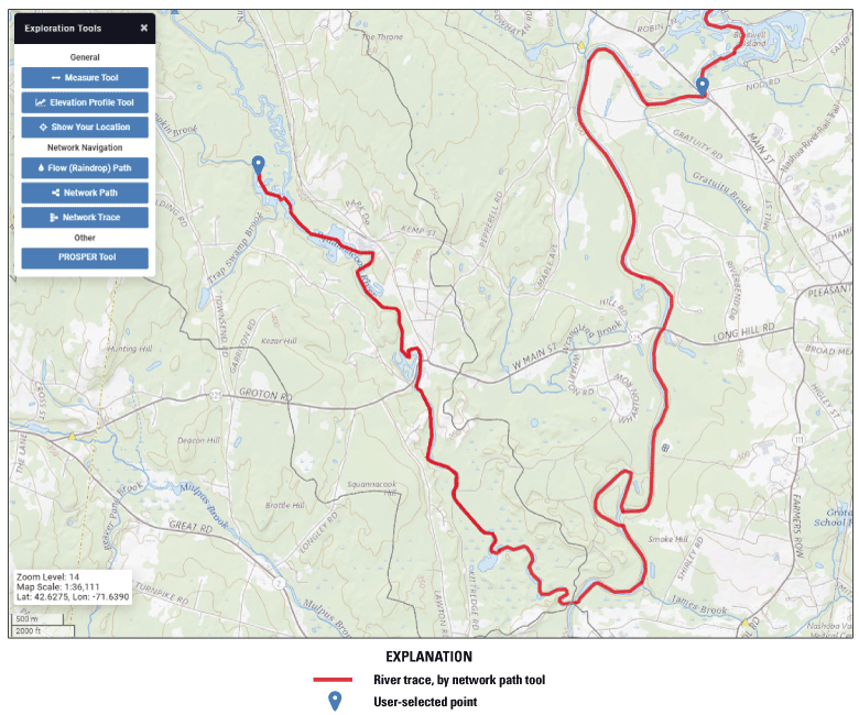
A screen capture of the StreamStats version 4 map frame with the results from use of the Network Path tool to highlight the path between two user-selected points on the stream network, indicated as blue pointers on the map. The latitude and longitude in the box in the lower left are coordinates for the center of the map frame.
Since the beginning of the development of StreamStats, the computer hardware and software needed to keep StreamStats operational have had to be continually evaluated. New hardware purchases were made when existing equipment broke or became obsolete and when additional capacity was required because more States were being added. StreamStats version 1 was initially implemented by using three servers in the Idaho USGS office—one for ArcIMS, one for ArcMap, and a data server running ArcSDE—that were linked together. As more States were added, the number of servers increased, and their processing and storage capacities also increased. The servers were moved from Idaho to the USGS National Geospatial Operations Center in Denver, Colorado, in 2006 when seven servers were in operation to take advantage of the greater internet data capacity that was available. By 2015, 18 servers were needed to operate StreamStats. With the transition to version 4 in 2016, StreamStats was fully migrated to commercial cloud services. The move to cloud services allowed computer resources to be available on demand and managed by the provider, reduced StreamStats team maintenance costs, and boosted reliability.
The StreamStats team has migrated its infrastructure from a single application with multiple web services behind it to an ecosystem of services, including multiple services and client applications (fig. 20). This architecture allows for faster and more efficient programming and enables StreamStats functionality to be used as web services in other applications without having to tap into the full StreamStats user interface. In turn, this approach facilitates fast and efficient development of additional tools and applications.
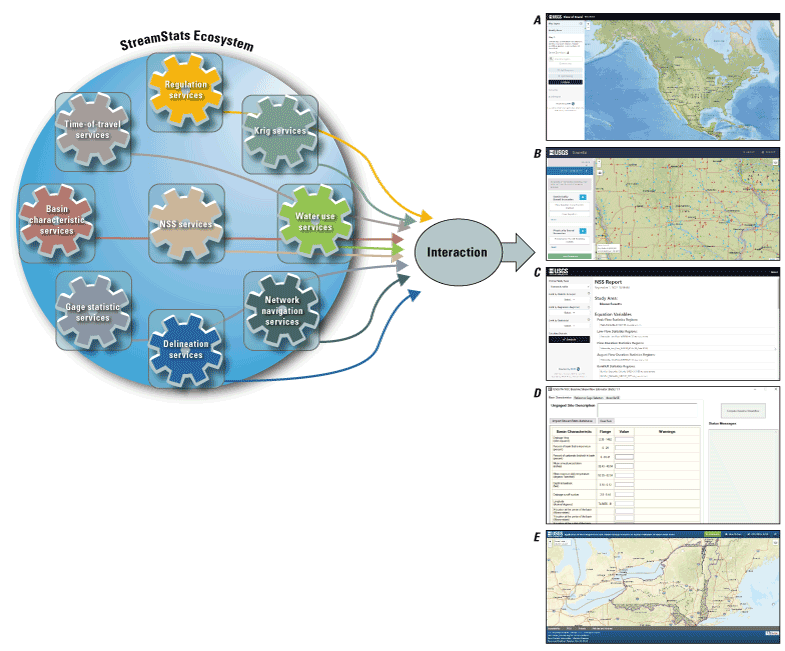
Diagram and screen captures showing the updated StreamStats computing architecture as an ecosystem of web services (left, only some services shown) that can be accessed for use in other applications (represented by screen captures on right) instead of in the StreamStats user interface.
Accommodating States that want to use lidar-based geospatial data also has been a challenge, both in providing guidance on data-preparation methods and in handling datasets that are approximately 10 times more dense than standard datasets while maintaining adequate user response times. Applications with lidar-based data are available for South Carolina, metropolitan St. Louis, Missouri, and western North Carolina and are in preparation for other States.
Further StreamStats Enhancements
StreamStats has evolved in response to the needs of internal and external users and changes in technology. Some enhancements have been developed and are available for testing in beta format. Several additional enhancements could be implemented to improve efficiency and add or improve functionality for users.
Existing Efforts
A beta version of a time-of-travel client application (https://www.usgs.gov/tools/time-travel-beta-application) for the conterminous United States, based on StreamStats web services, can calculate the travel times between stream locations of real or hypothetical hazardous waste spills and downstream locations of concern based on the equations of Jobson (1996). This application provides maximum probable and most probable travel-time predictions through a pair of tools: the Spill Planning tool and the Spill Response tool.
The Spill Planning tool was designed to help emergency response personnel plan for a potential spill. The tool traces (searches along the stream channel) a specified distance upstream from a user-selected point, often a water-supply intake of interest. After the trace is completed, the user is asked to input a streamflow value, which is then used as input for the Jobson equations, and then the results are presented as a colorized display of accumulated travel times for each stream reach in relation to the selected point.
The Spill Response tool was designed for use in the event of an actual spill. This tool traces a line a specified distance downstream from a user-selected point, which is the location of the spill either on land or on a water feature, to an intake or streamgage of interest. After the line is traced, the user is asked to input a spill mass, recovery ratio (optional), and discharge. Travel times and a peak concentration are then computed for each reach, and the travel times are accumulated in the downstream direction. This tool also offers a line chart depicting travel times for the leading edge, peak, and trailing edge for each reach in the selected area. For large areas, a user may select a stream-reach group to reduce the number of reaches shown in the chart for better visibility.
Output from the time-of-travel application is made available to the user in a final, printable report, with options to include a map of the study area, tables with accumulated maximum probable and most probable travel times, a line chart, a custom title, optional notes, and the citation for Jobson’s (1996) report. Within the output report, the user also has the options to export table content to a CSV file or download spatial data as a GeoJSON file.
For internal modeling uses, the USGS needs StreamStats to have the ability to deliver results based on nationally consistent data, but StreamStats generally was built by using the best available data at the time when it was implemented for each State. A national application has been released in beta format by the USGS at https://streamstats.usgs.gov/national-beta/ that can delineate drainage basin boundaries and compute a small set of basin characteristics (drainage area, percent forest, and January minimum and maximum temperatures) anywhere in the conterminous United States using NHDPlus version 2 datasets and StreamStats toolsets.
The national StreamStats application incorporates a Fire Hydrology tool that provides information needed to assess changes in hydrology after wildfires. Two main effects of wildfires on hydrology are increased runoff and decreased water quality. In the burned area after a wildfire, there is greater potential for flooding, erosion, and stream habitat degradation (Neary and others, 2011). Transportation of sediment, along with increased nutrient and metal concentrations to public water supplies, can lead to higher water-treatment costs and has the potential to affect water availability. The Fire Hydrology tool integrates watershed delineation capabilities with fire perimeter and burn severity layers to calculate postburn peak flows and provides stream tracing to identify affected streams and streamgages. The Fire Hydrology tool can provide actionable intelligence to stakeholders in the wildland fire, local government, and science communities in a streamlined fashion.
A substantially improved replacement has been developed for the Estimate Flows Based on Similar Streamgaging Stations tool from version 2, but it has not yet been released. The version 2 tool provided flow estimates for ungaged sites based on the flow per unit of drainage area for a nearby streamgage, and it worked only when there was a streamgage with a drainage area that is between 0.5 and 1.5 times the drainage area for a selected ungaged site. The new tool removes this limitation and provides indicators of the errors associated with the flow estimates, which generally are lower than the errors provided by the version 2 tool.
Efforts to bridge the gap between hydrology and hydraulics are underway in Massachusetts and South Carolina. Massachusetts has a pilot study to modify StreamStats to deliver peak-flow (unit) hydrographs and then use those hydrographs to solve equations to compute peak flows through culverts at user-selected locations within a major river basin in Massachusetts (U.S. Geological Survey, 2022a). The resulting outputs would include graphical representations and tables of potential dimensions for a culvert at the user-selected location. The South Carolina effort would also deliver unit hydrographs and use the results to compute peak flows using the time-of-concentration method (U.S. Department of Agriculture, Natural Resources Conservation Service, 2021). Other ongoing efforts to enhance StreamStats include development of
-
• a client application to calculate sediment transport in Minnesota rivers based on an artificial intelligence/machine learning model;
-
• support for providing flow estimates from models other than regression equations, such as models developed by using machine learning or hierarchical modeling, and for weighting estimates from multiple types of models to provide final estimates with minimal error variance;
-
• development of indices to describe the effects of dams, stock ponds, and diversions, which could be used in regression analysis or other hydrologic modeling to improve the understanding of these alterations of streamflow in Wyoming;
-
• improving estimation of streamflow in the urban environment of the District of Columbia by incorporating high-resolution spatial datasets of storm drains, lidar-based elevations and streams, and locally provided impervious areas; and
-
• use of groundwater models in Massachusetts to generate explanatory variables for use in improving regression equations for estimating low-flow statistics.
Potential Further Improvements
Several enhancements could improve the availability of information from StreamStats and the speed of its delivery. Modifying the StreamStats infrastructure to further optimize the use of cloud technology could deliver better products faster. New capabilities could allow users to get flow-statistic estimates for anywhere within a delineated basin or a specified area rather than just where there are streams, obtain drainage areas for a line across the landscape, such as the edge of a field, or download the underlying data used for a computation.
Further developing the national StreamStats application that provides basin delineations and basin characteristics for user-selected sites using GIS data at a consistent scale nationally will rely on a strong partnership between the StreamStats development team and the USGS National Geospatial Program (NGP), which has a long-term goal of providing a national, seamless, integrated, geospatial framework for hydrologic analysis. With the creation of the 3DHP effort by the NGP, further efforts at developing the NHD and NHDPlus HR have ceased. Expansion of the capabilities of the national application will now rely on use of the 3DEP and 3DHP datasets as they are completed. These datasets will likely be used eventually to replace those used for State applications.
The USGS is developing the National Hydrologic Geospatial Fabric (NHGF) to provide a web-accessible system including a network of connected representations of rivers, lakes, and catchments, derived physical characteristics, analysis tools, and a community of practice for users. The NHGF is being built by using the best available geospatial data, much of it from the NGP. A provisional version of the NHGF system (Blodgett and Johnson, 2022) has been released. It is expected that the NHGF could develop web services through which users could access StreamStats, and the web services developed by the NHGF could be accessed by StreamStats to provide additional functionality.
Improvements to the underlying datasets used for StreamStats State applications would also have many benefits. These improvements would come from increases in the resolution and precision of elevation data derived from lidar and improved methods for hydro-enforcing stream locations through methods such as (1) using selective burning rather than full-stream burning, such as burning only at stream-road crossings; (2) use of precipitation-intensity values to compute volumes of water generated by specified precipitation events, and imposing those volumes on the digital land surface to determine when low areas are likely to contribute surface water (fill-spill volumes); and (3) enforcing surveyed (known) culvert locations. These kinds of improvements to the underlying StreamStats State datasets could likely be achieved through the combined efforts of the StreamStats team, GIS specialists in USGS water science centers, and NGP staff.
The scope and applicability of methods to get flow statistics anywhere could be broadened, particularly with an emphasis on small basins. Currently (2023), more than 50 percent of delineations requested through the StreamStats interface are for basins of less than 2.5 square miles. Because the USGS operates relatively few streamgages with basin areas of this size, regression equations for estimating flow statistics have limited applicability for these small basins. Broadening the use of alternative methods for computing peak flows for small basins, such as the TR–55, the rational, and the time-of-concentration methods, would be helpful to many StreamStats users.
Further efforts to bridge the gap between hydrology and hydraulics could be made, including (1) developing the ability to use multiple resolutions of elevation data, such that higher resolution data could be used near stream channels for hydraulics computations and lower resolution data used elsewhere within a delineated basin; (2) enhancing tools for computing channel cross sections and profiles; (3) adding a tool for computing channel roughness; (4) linking to databases of hydraulic structures; (5) linking to flood-inundation models; (6) linking to NHGF river corridors and geomorphology data; (7) linking to fill-spill tools for determining volumes needed to spill over roadways; and (8) expanding linkage of basin hydrograph computations with culvert-flow computations.
Additional enhancements could include incorporating flow networks through karst areas and the development of additional transboundary and international applications. Implementation for the Lake of the Woods–Rainy River Basin showcases efforts at harmonization of geospatial data between two nations. Work that has already been completed to harmonize basin boundaries and stream networks for other river basins along the United States-Canadian border, including the Souris River Basin, Milk River Basin, and Kootenai River Basin (all in the western border region), and St. John River Basin (along the Maine border with Quebec and New Brunswick), could be leveraged to implement StreamStats for those basins. Existing methods and infrastructure also could be used to implement StreamStats for other nations.
SMARTStats
The USGS Water Mission Area prepared an internal plan in 2020 to develop an operational process for creating, publishing, and visualizing streamflow statistics that would be computed and released in a nationally consistent manner and on a much more frequent basis compared to past practices, where peak-flow statistics often were computed on average only about once in 10 years and low-flow statistics often were computed even less frequently. The plan would (1) establish a process for computing and routinely updating 60 interpretive and noninterpretive streamflow statistics that are representative of the full range of flows; (2) develop a national streamflow statistics database for the estimated flows and serve these data to the public; (3) use machine learning and hierarchical modeling to regionalize flow statistics; (4) provide estimates of flow statistics for each NHDPlus stream reach in the conterminous United States; and (5) develop a system for publishing relevant visualization products, such as tables and interactive maps, to allow spatial comprehension and analysis of the streamflow statistics. This planned system was named SMARTStats.
The SMARTStats plan would address weaknesses in the StreamStats approach that limit the usefulness of StreamStats-provided information for large, regional analyses. StreamStats relies on a cooperative model for computing streamflow statistics and generating estimates at ungaged sites through use of regression analysis. Consequently, the statistics available through StreamStats are inconsistent in type and currency among the States. Also, over the decades when they have been used by the USGS, the methods of performing regression analyses have improved, so newer machine learning and hierarchical modeling techniques hold promise for delivering superior estimates. Although SMARTStats would address these weaknesses of StreamStats, StreamStats provides substantial additional functionality and custom processes developed for several States that SMARTStats would not address.
A team was established in 2021 to review the SMARTStats plan and identify potential effects of its implementation on internal and external stakeholders, recommend revisions to the plan, and provide an implementation strategy. The review team released 13 findings after evaluating feedback from numerous stakeholder meetings, including that (1) SMARTStats should become part of the ecosystem of services in the planned StreamStats platform architecture, (2) StreamStats should be reconfigured to allow seamless access to both the SMARTStats nationally consistent statistics and those produced by the State offices, and (3) the SSAC should be reconstituted to provide guidance to the team. These recommendations and several others from the review team, as well as the SMARTStats plan itself, will likely have a major effect on how StreamStats operates in the future. The SMARTStats plan did not foresee the development of the 3DHP or the NHGF, and so the plan will likely need to be modified to accommodate the data that will be generated by these programs.
Lessons Learned
The development, implementation, and nearly a quarter century of operation of StreamStats have provided major lessons, which may be useful to others who consider undertaking efforts of similar complexity:
-
1. Finding allies among potential internal and external stakeholders was essential to gaining support for initiating the project.
-
2. Teamwork is essential when undertaking complex projects such as StreamStats. Team members bring a mix of expertise and experience that no one person can have and lead to better outcomes. Cross-training of team members is important to prevent a sudden loss of expertise if a team member leaves or is temporarily unable to contribute.
-
3. Extensive planning, budgeting, and oversight are needed to assure that projects are completed on time and within budget, but expect to adaptively manage and change plans along the way in response to possible delays or unanticipated additional costs.
-
4. Constantly communicate with potential internal and external stakeholders to assure them of the benefits of the product, to get ideas for improvement, and to keep them informed of progress. Use outreach to inform potential new users of your product. Also, communicate with other relevant internal and external organizations to coordinate activities and exchange ideas.
-
5. The cooperative funding model used for implementing StreamStats substantially lowered the overall cost to the USGS by requiring other agencies to provide funding and assured that the product was relevant to local users, but the funding model increased the time needed for full implementation by several years.
-
6. The StreamStats design model allowed flexibility in the scales of the GIS data used for implementation, the map projections, and the supporting map layers. This flexible approach made it easier to satisfy the wants and needs of local cooperators, allowed use of the best data available for a given area, and allowed for the addition of custom functionality. A standard implementation approach was not possible when the national StreamStats effort began because of a lack of relevant national GIS datasets. If standardized datasets had been available, implementation would have required less effort and resulted in greater consistency in appearance across State lines. However, the flexible approach allowed higher resolution data to be used in places where they were available and probably resulted in greater innovation than would have occurred with a standardized approach.
-
7. Getting GIS specialists in the local USGS offices involved in generating the geospatial datasets needed to implement StreamStats benefitted the local offices by increasing the expertise of their GIS specialists, often allowing those specialists to take on more complex and innovative follow-on work. StreamStats team GIS specialists also benefitted from innovations introduced by the local GIS specialists.
-
8. The StreamStats development team often was asked to provide improvements on existing functionality and add new functionality, and usually, a strong case could be made for doing so. However, sometimes it was not possible to accomplish the requested work within available time and funding constraints, and it was necessary to say that either the work could not be done, or it would have to wait until more resources were available.
-
9. Use internal expertise whenever possible to avoid contracting delays and maintain optimal control of the work.
-
10. Events beyond your control will cause delays and reprioritization of work, but these events also can lead to product improvements. For example, a higher resolution stream network became available for a State after much of the needed data for it had already been processed by using a lower resolution stream network. In consultation with the State cooperator, the team decided to start again using the higher resolution stream network so that the final product would be more accurate. Incorporating a margin for error in budgets and timelines for unplanned contingencies is advisable.
-
11. StreamStats provides a prime example of innovation begetting innovation. Many functionalities were added over time because of users who could see the utility of StreamStats but wanted it to do more, and these users were willing to work with the development team to make it happen.
Summary
Estimates of streamflow statistics, such as the 1-percent annual exceedance probability peak flow, the mean flow, and the 7-day, 10-year low flow, have been used for many decades in a variety of studies and applications. Some uses of streamflow statistics include the design of structures over, on, or near water, such as roads, bridges, water supplies, wastewater-treatment plants, power-generation stations, and factories; delineation of floodplains for land-use zoning and setting of insurance rates; and hydrologic and climate change studies. Streamflow statistics can be determined at streamgage locations from available data, but streamgage locations represent only a very small proportion of the possible locations where streamflow statistics could be needed.
The U.S. Geological Survey (USGS) has been using regression analysis since at least the early 1960s to generate equations that can be used to estimate streamflow statistics at ungaged sites. These equations are developed by statistically relating computed streamflow statistics to selected physical and climatic characteristics of the drainage basins for a group of streamgages. Streamflow statistics for an ungaged site can be estimated by first computing the basin characteristics and then inserting them into the equations. For many years, an impediment to the use of regression equations for estimating streamflow statistics at ungaged sites was the need for users to determine the basin characteristics used as explanatory variables in the equations. The same source data and methods must be used to compute the basin characteristics, or the resulting estimates of streamflow statistics may be biased or have reduced accuracy. Many potential users did not have the source maps, equipment, or expertise needed to determine the basin characteristics accurately, and the time required to determine the basin characteristics was cost prohibitive.
Three basin yield studies were done by the USGS in Massachusetts in the 1990s to develop regression equations for estimating low-flow statistics. These studies took advantage of the then-emerging field of GIS technology to determine basin characteristics needed for the streamgages used in the studies. A computer program named ONEBASIN was written to automate the process of computing the basin characteristics for all the streamgages. This automation of the GIS process allowed for a major advance in the efficiency of computing basin characteristics and made the computed values more reproducible. However, a problem with this approach was that few potential users of the resulting regression equations had the GIS capabilities required to duplicate the methods needed to compute the basin characteristics appropriately.
By the time the final basin yield study began in 1998, computer processing speeds and internet technology had advanced to the point that allowed the study to include an effort to create a web-based geographic information system (GIS) application so online users could obtain estimates of low-flow statistics at user-selected ungaged sites, and to allow users to get previously published estimates of streamflow statistics for streamgages. The ONEBASIN desktop program was modified to work on the web within a custom-built, map-based user interface that allowed users to move around the map to identify a location of interest, initiate the process of delineating the basin boundary, compute basin characteristics, and solve the regression equations to generate estimates of the streamflow statistics for the selected site. This application, named Massachusetts StreamStats, was formally released in 2001 and was the first known web-based application with interactive geoprocessing.
The release of Massachusetts StreamStats led to strong interest in the availability of similar products for other States and, as a result, the USGS began an effort in 2001 to develop a StreamStats application that could be implemented nationally. The USGS created a team to develop the new application, to develop GIS data-preparation standards, and to train and assist USGS State office personnel with data preparation. The ONEBASIN-based process and data-preparation methods became the national model for StreamStats and also were adopted to develop other national datasets, such as the National Hydrography Dataset Plus (NHDPlus).
In 2005, Idaho became the first State available in the national version of StreamStats. The addition of individual States has relied on cooperative funding agreements with other Federal or State agencies to provide at least half of the data-preparation cost, so StreamStats still has not been implemented for a few States.
A major challenge in operating StreamStats for nearly a quarter century has been the need to continually keep up with changes in computer, web, and GIS technology. New versions of the software on which StreamStats is reliant have resulted in multiple instances of the need to replace or make major modifications to the StreamStats code. These changes have been costly and time consuming but have resulted in improvements to StreamStats over time. Additional modifications to the StreamStats code made over the years, usually at the request of cooperating agencies, have added functionality that is available nationally or regionally. Cooperating agencies from several States also have requested custom functionality that has been implemented in StreamStats or in separate applications that are linked to StreamStats.
The StreamStats development team has made several enhancements available publicly as beta applications and has identified several additional enhancements to further improve performance and add functionality, including development of a national application that uses consistent-scale data (NHDPlus version 2) to provide consistent results for anywhere in the conterminous United States. A new USGS initiative, named SMARTStats, will likely lead to major changes in the way StreamStats works. Lessons learned through the operation of StreamStats could be of benefit to others who consider undertaking efforts of similar scope.
“StreamStats in Pennsylvania is relied upon for water withdrawal and wastewater discharge permit applications and infrastructure design calculations. Pennsylvania Department of Environmental Protection (PADEP) staff and consultants preparing applications use StreamStats on a regular basis to delineate watersheds and to determine flow statistics and basin characteristics for that specific delineated watershed. PADEP has developed an internal process to access information and data from StreamStats [StreamStats services]. In addition, PADEP uses StreamStats for Statewide water planning activities for managing water resources.”
—Pennsylvania Department of Environmental Protection (written communication to Marla Stuckey, USGS, February 17, 2021)
References Cited
Agafonkin, V., 2022, Leaflet—an open-source JavaScript library for mobile-friendly interactive maps, version 1.0: Leaflet web page, accessed April 10, 2023, at https://leafletjs.com/.
Archfield, S.A., and Steeves, P.A., 2012, User manual for the Connecticut River UnImpacted Streamflow Estimation (CRUISE) tool, version 1.3 (last updated July 2013): U.S. Geological Survey user manual, accessed April 10, 2023, at https://www.usgs.gov/media/files/usersmanualcruise.
Archfield, S.A., Steeves, P.A., Guthrie, J.D., and Ries, K.G., III, 2013, Towards a publicly available, map-based regional software tool to estimate unregulated daily streamflow at ungauged rivers: Geoscientific Model Development, v. 6, no. 1, p. 101–115, accessed April 10, 2023, at https://doi.org/10.5194/gmd-6-101-2013.
Blodgett, D., and Johnson, M., 2022, Progress toward a reference hydrologic geospatial fabric for the United States: U.S. Geological Survey Water Data For the Nation blog, first posted December 12, 2022; accessed March 28, 2023, at https://waterdata.usgs.gov/blog/hydrofabric/.
Dalrymple, T., 1960, Flood-frequency analyses, manual of hydrology—Part 3: U.S. Geological Survey Water-Supply Paper 1543–A, 80 p. [Also available at https://doi.org/10.3133/wsp1543A.]
Dhakal, N., 2012, Development of guidance for runoff coefficient selection and modified rational unit hydrograph method for hydrologic design: Auburn, Ala., Auburn University, Ph.D. dissertation, 161 p., accessed April 10, 2023, at https://etd.auburn.edu/xmlui/handle/10415/3105.
Esri Water Resources Team, 2014, Arc Hydro 10.2—Overview document #1: Redlands, Calif., Esri, 26 p., accessed March 15, 2023, at https://community.esri.com/t5/water-resources-documents/arc-hydro-10-2-overview-document-1/ta-p/910485?attachment-id=50086.
Farmer, W.H., Kiang, J.E., Feaster, T.D., and Eng, K., 2019, Regionalization of surface-water statistics using multiple linear regression: U.S. Geological Survey Techniques and Methods, book 4, chap. A12, 40 p., accessed March 15, 2023, at https://doi.org/10.3133/tm4A12.
Feaster, T.D., Clark, J.M., and Kolb, K.R., 2018, StreamStats for South Carolina—A multipurpose water-resources web application: U.S. Geological Survey Fact Sheet 2018–3070, 4 p., accessed March 15, 2023, at https://doi.org/10.3133/fs20183070.
Hellweger, F., 1997, AGREE–DEM surface reconditioning system: Austin, Tex., The University of Texas at Austin, Civil, Architectural, and Environmental Engineering, Center for Water and the Environment web page, accessed April 10, 2023, at https://www.ce.utexas.edu/prof/maidment/gishydro/ferdi/research/agree/agree.html.
Hutchinson, M.F., 1989, A new procedure for gridding elevation and stream line data with automatic removal of spurious pits: Journal of Hydrology, v. 106, no. 3–4, p. 211–232. [Also available at https://doi.org/10.1016/0022-1694(89)90073-5.]
Hutchinson, M.F., 2011, ANUDEM version 5.3 user guide: Canberra, Australia, The Australian National University Fenner School of Environment and Society, 26 p., accessed April 10, 2023, at https://fennerschool.anu.edu.au/files/usedem53_pdf_16552.pdf.
Jaeger, K.L., Sando, T.R., McShane, R.R., Dunham, J.B., Hockman-Wert, David, Kaiser, K.E., Hafen, Konrad, Risley, John, and Blasch, Kyle, 2019, Probability of Streamflow Permanence Model (PROSPER)—A spatially continuous model of annual streamflow permanence throughout the Pacific Northwest: Journal of Hydrology, v. 2, article 100005, 19 p., accessed April 10, 2023, at https://doi.org/10.1016/j.hydroa.2018.100005.
Jobson, H.E., 1996, Prediction of traveltime and longitudinal dispersion in rivers and streams: U.S. Geological Survey Water-Resources Investigations Report 96–4013, 69 p. [Also available at https://doi.org/10.3133/wri964013.]
Johnston, C.M., Dewald, T.G., Bondelid, T.R., Worstell, B.B., McKay, L.D., Rea, A., Moore, R.B., and Goodall, J.L., 2009, Evaluation of catchment delineation methods for the medium-resolution National Hydrography Dataset: U.S. Geological Survey Scientific Investigations Report 2009–5233, 88 p. [Also available at https://doi.org/10.3133/sir20095233.]
McKay, L., Bondelid, T., Dewald, T., Johnston, J., Moore, R., and Rea, A., 2012, NHDPlus Version 2—User guide (March 13, 2019, version; data model version 2.1): U.S. Environmental Protection Agency, 182 p., accessed January 9, 2024, at https://www.epa.gov/system/files/documents/2023-04/NHDPlusV2_User_Guide.pdf.
Moore, R.B., Johnston, C.M., Robinson, K.W., and Deacon, J.R., 2004, Estimation of total nitrogen and phosphorus in New England streams using spatially referenced regression models: U.S. Geological Survey Scientific Investigations Report 2004–5012, 50 p. [Also available at https://doi.org/10.3133/sir20045012.]
Neary, D.G., Koestner, K.A., and Youberg, A., 2011, Hydrologic impacts of high severity wildfire—Learning from the past and preparing for the future, in 24th Annual Symposium of the Arizona Hydrological Society, Watersheds near and far—Response to changes in climate and landscape, September 18–20, 2010, Flagstaff, Ariz.: Arizona Hydrological Society, 8 p. [Also available at https://www.fs.usda.gov/rm/pubs_other/rmrs_2011_neary_d003.pdf.]
Olson, S.A., and Norris, J.M., 2005, U.S. Geological Survey streamgaging from the National Streamflow Information Program: U.S. Geological Survey Fact Sheet 2005–3131, 4 p. [Also available at https://doi.org/10.3133/fs20053131.]
Peters, D., 2015, The evolution of GIS software: Redlands, Calif., Esri Press, 2 p., accessed April 9, 2023, at https://www.esri.com/about/newsroom/wp-content/uploads/2018/10/the-evolution-of-gis-software.pdf.
Ries, K.G., III, 1994a, Development and application of generalized-least-squares regression models to estimate low-flow duration discharges in Massachusetts: U.S. Geological Survey Water Resources Investigations Report 94–4155, 33 p. [Also available at https://doi.org/10.3133/wri944155.]
Ries, K.G., III, 1994b, Estimation of low-flow duration discharges in Massachusetts: U.S. Geological Survey Water-Supply Paper 2418, 50 p. [Also available at https://doi.org/10.3133/wsp2418. Supersedes USGS Open-File Report 93–38.]
Ries, K.G., III, 1999, Streamflow measurements, basin characteristics, and streamflow statistics for low-flow partial-record stations operated in Massachusetts from 1989 through 1996: U.S. Geological Survey Water Resources Investigations Report 99–4006, 162 p. [Also available at https://doi.org/10.3133/wri994006.]
Ries, K.G., III, 2007, The national streamflow statistics program—A computer program for estimating streamflow statistics for ungaged sites: U.S. Geological Survey Techniques and Methods 4–A6, 37 p. [Also available at https://doi.org/10.3133/tm4A6.]
Ries, K.G., III, and Friesz, P.J., 2000, Methods for estimating low-flow statistics for Massachusetts streams: U.S. Geological Survey Water Resources Investigations Report 00–4135, 81 p. [Also available at https://doi.org/10.3133/wri004135.]
Ries, K.G., III, and Steeves, P.A., 1991, A geographic information system program for estimating low-streamflow statistics in Massachusetts, in 27th Annual Conference, “Water management of river systems,” and symposium, “Resource development of the lower Mississippi River,” New Orleans, La., September 8–13, 1991: American Water Resources Association, p. 287–289.
Ries, K.G., III, Steeves, P.A., Freeman, A., and Singh, R., 2000, Obtaining streamflow statistics for Massachusetts streams on the World Wide Web: U.S. Geological Survey Fact Sheet 104–00, 4 p. [Also available at https://doi.org/10.3133/fs10400.]
Sanocki, C.A., Williams-Sether, T., Steeves, P.A., and Christensen, V.G., 2019, Techniques for estimating the magnitude and frequency of peak flows on small streams in the binational U.S. and Canadian Lake of the Woods–Rainy River Basin upstream from Kenora, Ontario, Canada, based on data through water year 2013: U.S. Geological Survey Scientific Investigations Report 2019–5012, 17 p., accessed April 9, 2023, at https://doi.org/10.3133/sir20195012.
Southard, R.E., 2010, Estimating the magnitude and frequency of floods in urban basins in Missouri: U.S. Geological Survey Scientific Investigations Report 2010–5073, 27 p. [Also available at https://doi.org/10.3133/sir20105073.]
Southard, R.E., Haluska, T., Richards, J.M., Ellis, J.T., Dartiguenave, C., and Djokic, D., 2020, Missouri StreamStats—St. Louis County and the City of St. Louis urban application: U.S. Geological Survey Scientific Investigations Report 2020–5040, 27 p., 1 app., accessed April 9, 2023, at https://doi.org/10.3133/sir20205040.
Steeves, P.A., 2002, NHD Watershed tool—Instructions for preprocessing supporting data layers: U.S. Geological Survey National Hydrography web page, accessed April 9, 2023, at https://nhd.usgs.gov/watershed/watershed_tool_inst_TOC.html#Toc474479741.
Stuckey, M.H., and Ulrich, J.E., 2016, User’s guide for the Delaware River Basin streamflow estimator tool (DRB–SET): U.S. Geological Survey Open-File Report 2015–1192, 6 p., accessed April 9, 2023, at https://doi.org/10.3133/ofr20151192.
U.S. Department of Agriculture, Natural Resources Conservation Service, 2021, Estimating runoff volume and peak discharge, chap. 2 of Part 650—engineering field handbook: U.S. Department of Agriculture, Natural Resources Conservation Service, National Engineering Handbook, p. 650–2.19—650–2.22, accessed March 15, 2023, at https://directives.sc.egov.usda.gov/OpenNonWebContent.aspx?content=46253.wba.
U.S. Department of Agriculture, Soil Conservation Service, 1986, Urban hydrology for small watersheds: U.S. Department of Agriculture, Soil Conservation Service, Technical Release 55, 164 p., accessed March 15, 2023, at https://openlibrary.org/books/OL25931549M/Urban_hydrology_for_small_watersheds.
U.S. Environmental Protection Agency, 2020, NHDPlus (National Hydrography Dataset Plus): U.S. Environmental Protection Agency web page, accessed March 15, 2023, at https://www.epa.gov/waterdata/nhdplus-national-hydrography-dataset-plus.
U.S. Geological Survey, 2016, The Delaware River Basin Streamflow Estimator Tool (DRB–SET): U.S. Geological Survey Software Releases web page, accessed March 15, 2023, at https://www.usgs.gov/software/delaware-river-basin-streamflow-estimator-tool-drb-set.
U.S. Geological Survey, 2019, National Streamflow Statistics Program (NSS): U.S. Geological Survey Software Releases web page, accessed March 16, 2023, at https://www.usgs.gov/software/national-streamflow-statistics-program-nss.
U.S. Geological Survey, 2020a, 3D Elevation Program: U.S. Geological Survey web page, accessed March 15, 2023, at https://www.usgs.gov/core-science-systems/ngp/3dep.
U.S. Geological Survey, 2020b, National Hydrography Dataset: U.S. Geological Survey National Hydrography web page, accessed March 15, 2023, at https://www.usgs.gov/national-hydrography/national-hydrography-dataset.
U.S. Geological Survey, 2021, Hydrologic unit codes (HUCs) explained: U.S. Geological Survey Nonindigenous Aquatic Species web page, accessed March 15, 2023, at https://nas.er.usgs.gov/hucs.aspx.
U.S. Geological Survey, 2022a, A statewide hydraulic modeling tool for stream crossing projects in Massachusetts: U.S. Geological Survey web page, accessed April 8, 2023, at https://www.usgs.gov/centers/new-england-water-science-center/science/a-statewide-hydraulic-modeling-tool-stream.
U.S. Geological Survey, 2022b, USGS surface-water data for the Nation: U.S. Geological Survey National Water Information System database, accessed March 15, 2023, at https://doi.org/10.5066/F7P55KJN. [Surface-water data available at https://waterdata.usgs.gov/nwis/sw.]
U.S. Geological Survey, 2023a, NHDPlus High Resolution: U.S. Geological Survey web page, accessed March 15, 2023, at https://www.usgs.gov/core-science-systems/ngp/national-hydrography/nhdplus-high-resolution.
U.S. Geological Survey, 2023b, The 3D National Topography Model call for action—Part 1—The 3D Hydrography Program: U.S. Geological Survey web page, accessed March 24, 2023, at https://www.usgs.gov/national-hydrography/3d-national-topography-model-call-action-part-1-3d-hydrography-program.
U.S. Geological Survey and U.S. Department of Agriculture, Natural Resources Conservation Service, 2013, Federal standards and procedures for the national Watershed Boundary Dataset (WBD) (4th ed.): U.S. Geological Survey Techniques and Methods, book 11, chap. A3, 63 p., accessed April 9, 2023, at https://doi.org/10.3133/tm11A34.
Watson, K.M., 2022, New Jersey StreamStats digital elevation, flow direction, and flow accumulation GIS data 2022: U.S. Geological Survey data release, accessed March 15, 2023, at https://doi.org/10.5066/P98KJAH9.
Weaver, J.C., Terziotti, S., Kolb, K.R., and Wagner, C.R., 2012, StreamStats in North Carolina—A water-resources web application: U.S. Geological Survey Fact Sheet 2012–3137, 4 p., accessed March 15, 2023, at https://doi.org/10.3133/fs20123137.
Abbreviations
3DEP
3D Elevation Program
3DHP
3D Hydrography Program
ACWI
Advisory Committee on Water Information
AML
ARC Macro Language
ArcIMS
ArcView Internet Map Server
CDOT
Colorado Department of Transportation
CRADA
cooperative research and development agreement
CRUISE
Connecticut River UnImpacted Streamflow Estimation tool
DEM
digital elevation model
DLG
digital line graph
DRB
Delaware River Basin
DRB–SET
Delaware River Basin Streamflow Estimation Tool
EPA
U.S. Environmental Protection Agency
EROS
Earth Resources Observation and Science [U.S. Geological Survey data center]
GIS
geographic information system
HUC
hydrologic unit code
lidar
light detection and ranging
MassGIS
Commonwealth of Massachusetts Bureau of Geographic Information
MDEM
Commonwealth of Massachusetts Department of Environmental Management
NED
National Elevation Dataset
NFF
National Flood Frequency [program]
NGP
National Geospatial Program
NHD
National Hydrography Dataset
NHDPlus
National Hydrography Dataset Plus
NHDPlus HR
high-resolution version of NHDPlus
NHGF
National Hydrologic Geospatial Fabric
NRCS
National Resources Conservation Service
NSS
National Streamflow Statistics [program]
PROSPER
Probability of Streamflow Permanence [model]
SPARROW
Spatially Referenced Regressions on Watershed Attributes [model]
SSAC
StreamStats Advisory Committee
USGS
U.S. Geological Survey
WBD
Watershed Boundary Dataset
For more information about this report, contact
National StreamStats Coordinator
U.S. Geological Survey
1728 Lampman Drive, Suite D
Billings, MT 59102
406-475-4585
Disclaimers
Any use of trade, firm, or product names is for descriptive purposes only and does not imply endorsement by the U.S. Government.
Although this information product, for the most part, is in the public domain, it also may contain copyrighted materials as noted in the text. Permission to reproduce copyrighted items must be secured from the copyright owner.
Suggested Citation
Ries, K.G., III, Steeves, P.A., and McCarthy, P., 2024, StreamStats—A quarter century of delivering web-based geospatial and hydrologic information to the public, and lessons learned: U.S. Geological Survey Circular 1514, 40 p., https://doi.org/10.3133/cir1514.
ISSN: 2330-5703 (online)
ISSN: 1067-084X (print)
| Publication type | Report |
|---|---|
| Publication Subtype | USGS Numbered Series |
| Title | StreamStats—A quarter century of delivering web-based geospatial and hydrologic information to the public, and lessons learned |
| Series title | Circular |
| Series number | 1514 |
| DOI | 10.3133/cir1514 |
| Publication Date | March 13, 2024 |
| Year Published | 2024 |
| Language | English |
| Publisher | U.S. Geological Survey |
| Publisher location | Reston, VA |
| Contributing office(s) | WMA - Integrated Modeling and Prediction Division |
| Description | viii, 40 p. |
| Online Only (Y/N) | N |
| Additional Online Files (Y/N) | N |