

Calibrating Optical Turbidity Measurements with Suspended-Sediment Concentrations from the Herring River in Wellfleet, Massachusetts, from November 2018 to November 2019
Links
- Document: Report (4.57 MB pdf) , HTML , XML
- Data Releases:
- USGS data release - Suspended-sediment concentrations and loss-on-ignition from water samples collected in the Herring River during 2018-19 in Wellfleet, MA (ver 1.1, March 2023)
- USGS data release - Time-series measurements of oceanographic and water quality data collected in the Herring River, Wellfleet, Massachusetts, USA, November 2018 to November 2019
- USGS data release - Water quality data from a multiparameter sonde collected in the Herring River during November 2018 to November 2019 in Wellfleet, MA
- NGMDB Index Page: National Geologic Map Database Index Page (html)
- Download citation as: RIS | Dublin Core
Acknowledgments
This study was supported by the U.S. Geological Survey (USGS) through the Coastal and Marine Hazards and Resources Program and the USGS and National Park Service through the Natural Resources Preservation Program.
Special thanks are given to USGS personnel, Jonathan Borden and Marinna Martini, for their participation in field work and sample collection, and Brian Buczkowski, manager of the Woods Hole Coastal and Marine Science Center Sediment Analysis Laboratory in Woods Hole, Massachusetts, for determining suspended-sediment concentrations.
Abstract
The sediment budget in the tidally restricted Herring River in Wellfleet, Massachusetts, must be quantified so restoration options for the river can be evaluated. Platforms equipped with optical turbidity sensors were deployed seaward and landward of the Herring River restriction to measure a time series of turbidity, from which a time series of suspended-sediment concentrations (SSCs) can be estimated. Water samples were collected periodically from the Herring River from November 2018 to November 2019 and analyzed for SSC to derive a relationship to turbidity measurements given in nephelometric turbidity units. This report presents the data-collection methods used and the linear calibration model generated by repeated median regression to convert turbidity measurements to SSC.
Introduction
The Herring River estuary system, composed of several tributary streams and basins, encompasses 1,100 acres along the Cape Cod National Seashore. The estuary system has experienced ecological degradation because of the construction of a dike at Chequessett Neck Road at the mouth of the Herring River in 1909 (Smith and others, 2020). The dike restricts tidal exchange, thus reducing sediment supply to the area upstream from the dike. This lack of sediment supply may lead to marsh loss because a steady import of sediment is necessary for accretion and lateral expansion of the marsh.
Smith and others (2020) have worked with the Herring River Restoration Committee to develop a decision framework for restoration that will represent the varied interests of multiple stakeholders, including scientists, aquaculture managers, and the adjacent residents. Ultimately, restoration managers seek to restore the natural hydrology and ecological function of the estuary by building a new tide-control system that will incrementally adjust the tidal range, while minimizing the socioeconomic effects that such construction might cause. Obtaining sediment flux baseline data before restoration is important to allow future changes stemming from the restoration to be evaluated. The objective of this report is to present the calibration model (generated by repeated median regression) used to convert turbidity measurements into estimates of suspended-sediment concentrations (SSC). The resulting time series of SSC can be used to calculate sediment transport flux within the system.
Sensor Deployment and Water Sample Collection
Two WET Labs ECO-NTU sensors (Sea-Bird Scientific, Bellevue, Washington), which had been calibrated in an eight-point Formazin dilution series from 0 to 500 nephelometric turbidity units (NTU), and two multiparameter YSI EXO2 sensors (Xylem, Inc., Yellow Springs, Ohio) which were factory-calibrated, were checked before deployment with a two-point calibration in the laboratory at 0 NTU (de-ionized water) and 126 NTU (YSI 6073G turbidity standard). The sensors were mounted on platforms between 0.15 and 0.40 meter above the sediment bed from November 12–15, 2018, at three sites seaward and one site landward of the Herring River restriction (fig. 1 and table 1). Continuous turbidity measurements were taken by these sensors at 15-minute intervals for approximately 1 year until November 19, 2019, except for when the ECO-NTU sensors at the flank shallow (FS) and flank deep (FD) sites were removed from January 16, 2019, to March 27, 2019, due to ice concerns at these intertidal locations. The sensors contain integrated wipers that wiped the optical lens before sampling to prevent biofouling. During the year, the sensors were recovered three times to replace the batteries and then re-deployed. Water samples to be analyzed for SSC were collected periodically during the deployment using a Van Dorn sampler: a 1-liter horizontal point sampler that collects a sample at a specific depth (Buchanan and others, 1996). The water samples were refrigerated in the dark after collection and filtered within 1 month. Turbidity readings were taken concurrently with the water samples using a YSI EXO2 sensor with a handheld display (EXOHH).
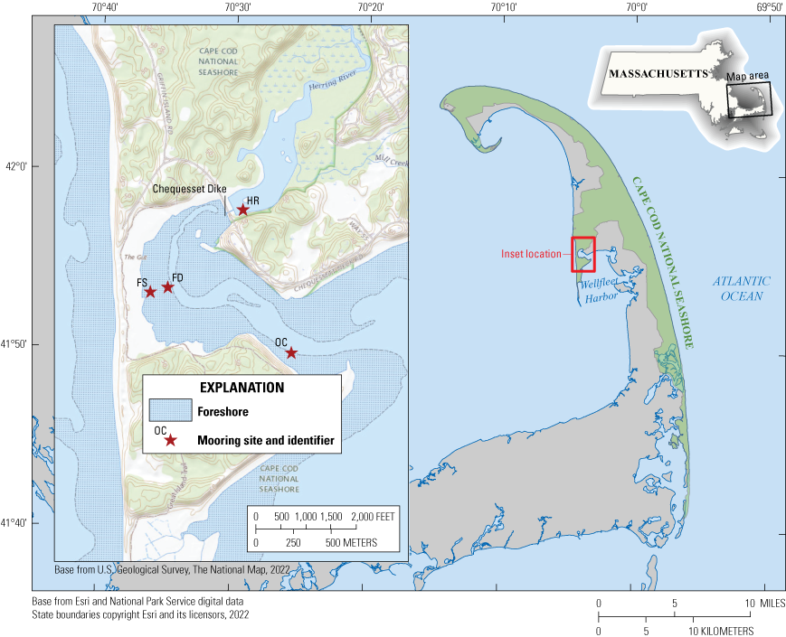
Map showing the Herring River turbidity sensor deployment sites.
Laboratory Determination of Suspended-Sediment Concentration
Water samples were filtered at the U.S. Geological Survey Woods Hole Coastal and Marine Science Center Sediment Analysis Laboratory in Woods Hole, Massachusetts. Glass-fiber filters (47-millimeter diameter with 1.5-micron pore sizes) were weighed and volatilized before filtering. The full volume of each water sample was filtered to avoid subsampling errors. If the solids load from a sample was too large to be filtered by a single filter, two or more filters were used. The filtrate was rinsed with de-ionized water to wash out dissolved salts, dried at 105 °C, and weighed (Ohaus AX224 micro-balance; Ohaus Corporation, Parsippany, New Jersey)—all steps following the methods in Fishman and Friedman (1989).
Calibration of the Optical Turbidity Sensor
Turbidity sensor values were downloaded from the EXOHH, and the times of the NTU readings were matched to the time the SSC water samples were collected. Values from a 10-second burst of the EXOHH were averaged to yield a single turbidity value. If no reading was taken with the EXOHH, the value from the deployed turbidity sensor reading within 10 minutes of the sample collection time was used. Table 2 shows the paired SSC and turbidity values for each sample collected. The “Date” and “Time (UTC)” columns refer to when the water sample was collected in Coordinated Universal Time (UTC), and the “SSC” column contains the laboratory-determined suspended-sediment concentration of the water sample. The “Sensor Turbidity (NTU)” column contains the turbidity measurement. The “Sensor” column shows whether the EXOHH or the deployed turbidity sensor was used to collect the turbidity measurement. The “Flag” column indicates whether data from the EXOHH were good (flag = 0), the reason the deployed sensor was used instead of the EXOHH, or why values were excluded from the calibration. Turbidity sensor values from the deployed sensor were used if no EXOHH values were collected (flag = 1) or if the EXOHH values failed to meet quality control criteria as follows: turbidity values from the EXOHH burst were eliminated if they were greater than 100 percent of the burst median turbidity value and less than 5 readings remained (flag = 2) or the standard deviation of the turbidity value divided by the mean turbidity value was greater than 0.5 (flag = 3). In some cases, no deployed sensor values were available, for instance when sampling stopped due to battery depletion (flag = 4). Deployed sensor values were excluded from the calibration if the standard deviation of the turbidity value divided by the mean turbidity value was greater than 0.5 (flag = 5). One water sample (July 25, 2019, 19:15 UTC) was eliminated from the calibration because the water sampler hit the riverbed (flag = 6) when the sample was captured and thus was not representative of the suspended sediment in the water column.
Table 2.
Suspended-sediment concentration and sensor turbidity for each water sample.[Data from De Meo and others (2023). Dates are shown as month–day–year. Time (UTC) is given in hour:minute:second. Flag values are defined as follows: 0 equals (=) good EXOHH data, 1 = deployed sensor values used (no EXOHH data), 2 = EXOHH values eliminated if greater than 100 percent of the burst median turbidity value and less than five readings remained, 3 = EXOHH values eliminated if the standard deviation of the turbidity value divided by the mean turbidity value was greater than 0.5, 4 = no deployed sensor values available, 5 = deployed sensor values excluded from calibration if the standard deviation of the turbidity value divided by the mean turbidity value was greater than 0.5, and 6 = water sample was eliminated from the calibration because the water sampler hit the riverbed. UTC, coordinated universal time; m, meter; SSC, suspended-sediment concentration; mg/L, milligrams per liter; NTU, nephelometric turbidity unit; OC, Outer Channel; HR, Herring River; EXOHH, YSI EXO2 sensor with a handheld display; FD, flank deep; FS, flank shallow; NaN, not a number; NA, not applicable]
Linear regression using a robust, nonparametric repeated median method (Siegel, 1982) was used to estimate SSC from turbidity. Repeated median estimates are less sensitive to the effects of outliers, so they were used as the regression method for the data in this study. The repeated median method calculates the slope of SSC versus sensor turbidity by determining the medians of all possible point-to-point slopes and then taking the median of those median slopes. The intercept was calculated as the median of all possible intercepts using the final slope calculation.
The nonparametric prediction interval (PInp), calculated as in Helsel and others (2020), is an error band containing one standard deviation (68 percent) of the calibration dataset. The PInp is not symmetric because it results from the distribution of the dataset. The PInp is calculated based on the residuals for each point, sorted from least to greatest. The 95-percent confidence interval of the slope was calculated as in Helsel and others (2020) by sorting all point-to-point slopes in ascending order. The ranks of the upper and lower intervals were then calculated and rounded to the nearest integer, and the slope associated with each rank was identified. See Buchanan and Lionberger (2007) for more detailed information about the PInp and confidence interval calculations that were used in this study.
Figure 2 displays the results of the repeated median regression, the nonparametric prediction interval, and the confidence interval. The calibration equation is
whereEighty data points were used to generate the equation. The nonparametric prediction interval ranged from +17 to −7, and the 95-percent confidence bounds on the slope calculation were 2.183 to 2.890. This equation will be used to derive a time series of SSC from the time series of deployed turbidity sensor data from Suttles and others (2023) to calculate sediment transport to or from marshes in the Herring River.
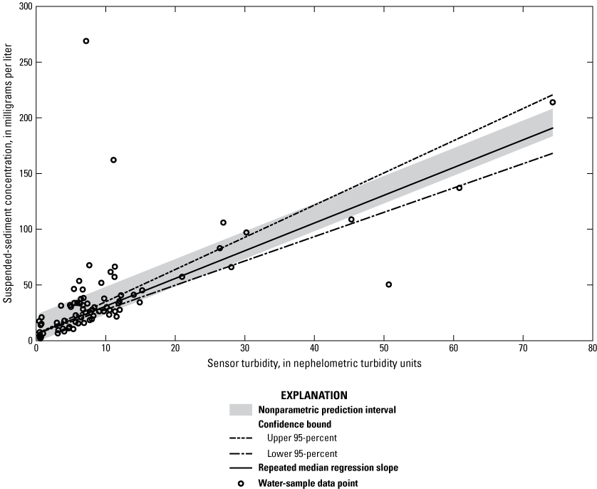
Graph showing the repeated median regression of suspended-sediment concentration versus sensor turbidity.
Summary
Two types of optical turbidity sensors were deployed at three sites seaward and one site landward of the Herring River restriction to monitor suspended sediment and characterize pre-restoration conditions in the river. Water samples were collected to determine suspended-sediment concentrations (SSCs) to calibrate the output of the sensors using robust, nonparameteric repeated median regression. The SSC data from the water samples and the measurements from the YSI EXO2 sensor with a handheld display are in De Meo and others (2022) and De Meo and others (2023), respectively. The resulting calibration model will be used with a time-series of deployed turbidity sensor data collected and reported by Suttles and others (2023) to derive a time series for SSC to input into sediment-flux calculations.
References Cited
Buchanan, P.A., and Lionberger, M.A., 2007, Summary of suspended-sediment concentration data, San Francisco Bay, California, water year 2005: U.S. Geological Survey Data Series 282, 46 p. [Also available at https://doi.org/10.3133/ds282.]
Buchanan, P.A, Schoellhamer, D.H., and Sheipline, R.C., 1996, Summary of suspended-solids concentration data, San Francisco Bay, California, water year 1994: U.S. Geological Survey Open-File Report 95–776, 48 p. [Also available at https://doi.org/10.3133/ofr95776.]
De Meo, O.A., Suttles, S.E., Ganju, N.K., and Marsjanik, E.D., 2022, Suspended-sediment concentrations and loss-on-ignition from water samples collected in the Herring River during 2018–19 in Wellfleet, MA (ver 1.1, March 2023): U.S. Geological Survey data release, accessed April 2023 at https://doi.org/10.5066/P9ZL2IPN.
De Meo, O.A., Suttles, S.E., Ganju, N.K., and Marsjanik, E.D., 2023, Water quality data from a multiparameter sonde collected in the Herring River during November 2018 to November 2019 in Wellfleet, MA: U.S. Geological Survey data release, accessed April 2023 at https://doi.org/10.5066/P9K3SCKY.
Fishman, M.J., and Friedman, L.C., 1989, Methods for determination of inorganic substances in water and fluvial sediments: U.S. Geological Survey Techniques of Water-Resources Investigations, book 5, chap. A1, 545 p. [Also available at https://doi.org/10.3133/twri05A1.]
Helsel, D.R., Hirsch, R.M., Ryberg, K.R., Archfield, S.A., and Gilroy, E.J., 2020, Statistical methods in water resources: U.S. Geological Survey Techniques and Methods, book 4, chap. A3, 458 p., accessed April 2023 at https://doi.org/10.3133/tm4A3.
Siegel, A.R., 1982, Robust regression using repeated medians: Biometrika, v. 69, no. 1, p. 242–244. [Also available at https://doi.org/10.1093/biomet/69.1.242.]
Smith, D.R., Eaton, M.J., Gannon, J.J., Smith, T.P., Derleth, E.L., Katz, J., Bosma, K.F., and Leduc, E., 2020, A decision framework to analyze tide-gate options for restoration of the Herring River Estuary, Massachusetts: U.S. Geological Survey Open-File Report 2019–1115, 42 p., accessed April 2023 at https://doi.org/10.3133/ofr20191115.
Suttles, S.E., De Meo, O.A., Ganju, N.K., Bales, R.D., and Marsjanik, E.D., 2023, Time-series measurements of oceanographic and water quality data collected in the Herring River, Wellfleet, Massachusetts, USA, November 2018 to November 2019: U.S. Geological Survey data release, accessed April 2023 at https://doi.org/10.5066/P95AE74D.
Datum
Horizontal coordinate information is referenced to the North American Datum of 1983 (NAD83).
Depth is referenced to the sea surface at time of sampling.
Supplemental Information
The data in this report were collected as part of a larger study, funded by the U.S. Geological Survey and National Park Service’s Natural Resources Preservation Program. This study encompasses four sites within the Northeast Coastal and Barrier Network: Cape Cod National Seashore, Fire Island National Seashore, Gateway National Recreation Area, and Assateague Island National Seashore. The overarching goals of this study are to identify the dominant sources of sediment, determine how sediment transport varies over time, and analyze sediment availability to marshes at the four sites to inform management efforts.
Concentrations of suspended sediment are given in milligrams per liter (mg/L).
For more information about this report, contact:
Director, Woods Hole Coastal and Marine Science Center
U.S. Geological Survey
384 Woods Hole Road
Quissett Campus
Woods Hole, MA 02543-1598
(508) 548–8700 or (508) 457–2200
WHSC_science_director@usgs.gov
or visit our website at
https://www.usgs.gov/centers/whcmsc
Publishing support provided by the
Pembroke and Baltimore Publishing Service Centers
Disclaimers
Any use of trade, firm, or product names is for descriptive purposes only and does not imply endorsement by the U.S. Government.
Although this information product, for the most part, is in the public domain, it also may contain copyrighted materials as noted in the text. Permission to reproduce copyrighted items must be secured from the copyright owner.
Suggested Citation
De Meo, O.A., Ganju, N.K., Bales, R.D., Marsjanik, E.D., and Suttles, S.E., 2023, Calibrating optical turbidity measurements with suspended-sediment concentrations from the Herring River in Wellfleet, Massachusetts, from November 2018 to November 2019: U.S. Geological Survey Data Report 1180, 8 p., https://doi.org/10.3133/dr1180.
ISSN: 2771-9448 (online)
Study Area
| Publication type | Report |
|---|---|
| Publication Subtype | USGS Numbered Series |
| Title | Calibrating optical turbidity measurements with suspended-sediment concentrations from the Herring River in Wellfleet, Massachusetts, from November 2018 to November 2019 |
| Series title | Data Report |
| Series number | 1180 |
| DOI | 10.3133/dr1180 |
| Publication Date | August 22, 2023 |
| Year Published | 2023 |
| Language | English |
| Publisher | U.S. Geological Survey |
| Publisher location | Reston, VA |
| Contributing office(s) | Woods Hole Coastal and Marine Science Center |
| Description | Report: vi, 8 p.; 3 Data Releases |
| Country | United States |
| State | Massachusetts |
| City | Wellfleet |
| Online Only (Y/N) | Y |
| Additional Online Files (Y/N) | N |