

A Synthesis Engine for Constructing Geologic Maps of the United States
Links
- Document: Report (9.42 MB pdf) , HTML , XML
- Table: Data Dictionary (52.0 KB csv)
- Data Releases:
- USGS data release - Cooperative National Geologic Map—Quaternary geology
- USGS data release - Cooperative National Geologic Map—Earth’s surface geology
- USGS data release - Cooperative National Geologic Map—Pre-Quaternary geology
- USGS data release - Cooperative National Geologic Map—Precambrian geology
- USGS data release - Geospatial database for the cooperative national geologic maps
- NGMDB Index Page: National Geologic Map Database Index Page (html)
- Download citation as: RIS | Dublin Core
Acknowledgments
This project was funded by the U.S. Geological Survey (USGS) National Cooperative Geologic Mapping Program. This work was made possible by the work of countless geologists in State Geological Surveys and the USGS to produce geologic maps and develop strategies and ideals for storing and compiling geologic map data. Andy Cyr, Dan Doctor, Ralph Haugerud, Kyle House, Jamey Jones, and Daven Quinn substantially improved this product through their thorough and thoughtful reviews of this text and associated derivatives. This report, and the products that come from it, would not have been possible without the unwavering devotion and drive of Jenna Shelton. From the beginning, Jenna has supported this work through her belief, energy, actions, and reasoning, all of which have shaped these products into maps of more magnitude and applicability. We thank Kat Sauer, Emily Martin, Sally Almeria, and Jeffrey Corbett for their diligent work on the text and visuals of this report, which have greatly aided its presentation.
Abstract
The geologic history of the United States is cataloged in thousands of geologic maps produced during many decades. However, the disparate nature of these individual maps makes it challenging to assess resources, research geologic histories, or characterize natural hazards holistically across the Nation. The U.S. House of Representatives 2020 appropriations bill for the U.S. Department of the Interior (H.R. 116-100) requires the U.S. Geological Survey to “bring together detailed national and continental-resolution [two-dimensional] and [three-dimensional] information produced throughout the Survey and by [F]ederal and [S]tate partners.” In response to this directive, this report presents a compilation and synthesis of geologic maps across the United States in the form of a relational database. The synthesis database includes thematic maps that synthesize the Nation’s geology, and retains the original input maps as well as linkages to standardized vocabularies to aid the discoverability of geologic information. Specifically, the synthesis database is targeted toward producing four National-resolution maps for the conterminous United States: Quaternary geology, the geology at the Earth’s surface, pre-Quaternary geology, and Precambrian geology. In addition, the synthesis database includes the infrastructure necessary to expand to additional resolutions in the future.
Introduction
The U.S. Geological Survey (USGS) National Cooperative Geologic Mapping Program (NCGMP) set forth the goal “* * * to create a variable-scale, National, integrated 2D [two-dimensional] and 3D [three-dimensional] geologic-framework model that enables the seamless construction of geologic maps * * * by the year 2030” (Brock and others, 2021, p. 6). The National Geologic Mapping Act of 1992 and subsequent reauthorizations (Public Law 102-285, as amended by Public Law 117-58) requires the USGS to “* * * expedite the production of a geologic-map database for the Nation, to be located within the United States Geological Survey” (U.S. Congress, 1992, 106 Stat. 167). House Report 116-100 directs the NCGMP to “* * * launch Phase Three of the National Geologic Map Database that will bring together detailed national and continental resolution 2D and 3D information produced throughout the Survey and by Federal and State partners” (U.S. Congress, House Appropriations Committee, 2020, p. 48–49; Shelton and others, 2022). Together, these directives require the USGS to create and maintain (1) a digital database, catalog, and archive of all geologic maps covering the United States (the National Geologic Map Database); and (2) a 2D and 3D geologic map of the Nation.
In service of the second of these directives, we designed a process and database structure for creating a new digital geologic map of the Nation that consists of a synthesis database containing many unmodified source maps, from which multiple map layers can be derived that portray different aspects of the Nation’s geology (Johnstone and others, 2025). The synthesis database is designed to rapidly “bring together” geologic maps in the Geologic Map Schema (GeMS) format (NCGMP, 2020). The original source data of each map is preserved, standardized using the Federal Geographic Data Committee (FGDC) cartographic standard (USGS, 2006), and integrated by assigning controlled, searchable vocabularies to map units.
From the synthesis database, source map data from many maps are composited into a set of visually and thematically consistent map layers, such as Quaternary geology in one layer, all units exposed at the Earth’s surface in another, and so on. Because the source data are unmodified, mismatches remain between source maps; that is, the layers are not geologically “seamless.” However, this approach facilitates very rapid assimilation of new maps and delivery of updates, unlike previous national maps that could only be updated by drafting new maps.
This report summarizes the programmatic goals and practical considerations that shaped the design of this new national synthesis map. We present the structure of the map synthesis database and the process for populating the synthesis database. We then demonstrate how integrated geologic map layers are derived from source maps in the synthesis database. Appendix 1 showcases potential uses of the synthesis database.
Goals and Background
Based on the legislative directives and programmatic goals described in the “Introduction” section, this national geologic map database must meet the following criteria:
-
• It is complete, covering the Nation, by the year 2030;
-
• It brings together maps produced by both the USGS and State geological surveys;
-
• It accommodates GeMS data as input and delivers GeMS data as output;
-
• It is capable of hosting multiple “resolutions,” herein interpreted as map scales or ranges of scales; and
-
• It is easily updated with new maps as they are published.
In the following sections, we discuss existing geologic maps of the United States that do not meet the above requirements but provide useful lessons on different compilation strategies and the utility of different products.
National Geologic Maps
The Reed and others (2005) Geologic Map of North America provides complete, seamless coverage of the conterminous United States and Alaska at a scale of 1:5,000,000. King and others (1974) provide more detailed, albeit more dated, coverage of the conterminous United States at a scale of 1:2,500,000. Both of these are traditional maps compiled by hand with attention to the final cartographic presentation and remain popular as visual depictions of the Nation’s geology (for example, Vigil and others, 2000; Barton and others, 2003). To present nationwide geology in a single map, both maps exclude Quaternary deposits from the Central and Northeastern United States but include them elsewhere, following a tradition of USGS national geologic maps going back to McGee (1884). Both maps took about two decades from start to publication; the King and others (1974) map was conceived in the 1950s (King and Beikman, 1974), and the 2005 Geologic Map of North America was instigated as part of the Decade of North American Geology in the early 1980s (Reed and others, 2005).
Map Compilation Databases
Colman-Sadd and others (1996) described the Reed and others (2005) and King and others (1974) maps as “compilations,” or the redrafting and interpretation of a typically reduced scale but internally consistent map, as distinct from “composition,” or the procedural assembly and aggregation of units at native scale. Colman-Sadd and others (1996) noted that composition maps accomplish many of the same goals as compilation maps except for the preservation of discontinuities in unit boundaries at the perimeters of some composited maps. The most recent digital “composition” of the conterminous United States is the State Geologic Map Compilation (SGMC) produced by the USGS Mineral Resources Program (Horton and others, 2017). It brings together 48 State geologic maps (one for each of the conterminous States) in a single database with minimal changes to their original content, which leaves mismatches across State borders but adds searchable lithologic attributes to make the data more accessible to queries. Like earlier paper maps, the SGMC does not include Quaternary geology in the Central and Northeastern parts of the United States. Nevertheless, as of 2024, it is widely distributed and used directly from the USGS and through third-party services. Although it now serves as a de facto national geologic map, the SGMC was created as input for mineral resource assessments and does not resemble a traditional map with an integrated set of map units that are differentiated by color and (or) patterns that can be visually read to understand the nation’s geologic history.
The Macrostrat platform expands further on the “composition” strategy by providing map data (including the SGMC) at multiple scales (Peters and others, 2018; Quinn and others, 2024). In addition to providing searchable attributes like the SGMC, Macrostrat further relates map units to one another through a network of stratigraphic columns, initially populated from the Correlation of Stratigraphic Units of North America (Childs, 1985). This approach allows Macrostrat to place source map units into a more unified stratigraphic framework and within integrated age model(s) in a platform built to evolve through time as a “living” integrator of geologic data (Quinn and others, 2024).
The Geologic Map of Alaska (Wilson and others, 2015) represents another innovation in map composition databases. As with the SGMC and Macrostrat, it preserves source map unit descriptions and assigns standardized, searchable attributes to source maps. However, it also takes care to preserve the core topology of the map (for example, the spatial relationships between map unit polygons, contacts, and faults) and the authors of the Geologic Map of Alaska use the database to relate all source map units to a common statewide stratigraphy, enabling a consistent statewide presentation legible as a traditional geologic map.
National Geologic Synthesis Map Design Philosophy
Although national maps compiled by traditional methods have nominally been superseded by more recent and information-rich digital compilations, they continue to demonstrate great value. These maps are frequently used in classrooms as teaching tools and in informational documents that communicate geology to the public. Since the publication of the SGMC in 2017, “traditional” national geologic maps, digital reproductions, and cartographic derivatives have been cited more than 175 times in formal publications as of November 1, 2024 (King and others, 1974; Schruben and others, 1994; Vigil and others, 2000; Barton and others, 2003; Reed and others, 2005; Garrity and Soller, 2009). From this use of traditional maps, we take the following lessons:
-
• Bringing together many maps without reinterpreting their original content—that is, making a composition—can yield a very useful product, even if interpretive mismatches remain between source maps;
-
• To make such a map efficient to update with new or revised maps, a standardized, automated procedure is necessary to avoid data integration becoming the rate-limiting factor in updates; and
-
• There is value in clear visual presentations of geologic map data, consistent with decades of precedent codified in USGS guides for geologic map color and symbology (USGS, 2005, 200635).
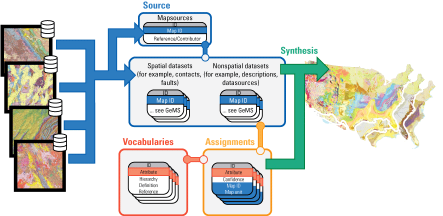
Figure 1 shows the general workflow created in response to these lessons. First, relevant maps produced in the GeMS format are ingested into the synthesis database without changing their interpretive content (fig. 1, step 1). Second, within the synthesis database, a process associates standardized attributes with original map units to facilitate analysis and discovery of geologic data, such as standardized age information (fig. 1, step 2). Third, maps are composited together as necessary to fill out the area of the synthesis (fig. 1, step 3). In some cases, this involves clipping out portions of maps before inserting others, but the full map is still preserved in the synthesis database; in other cases, this involves simply appending neighboring maps (for example, neighboring State geologic maps). These steps are comparable to the strategy undertaken to develop previous composite maps, both to produce a point-in-time product such as the SGMC (Horton and others, 2017) or to continually grow a “living” database as with Macrostrat (Peters and others, 2018; Quinn and others, 2024). Fourth, these previous approaches are extended by also offering a holistic synthesis of geology (fig. 1, step 4) that can be visually read as a single geologic map, with legends that resemble that of the Geologic Map of the United States and the Geologic Map of North America (King and others, 1974; Reed and others, 2005). This approach preserves both the original content of individual source publications and a generalized depiction of the geology that is consistent across input publications, similar to the strategy employed for the Geologic Map of Alaska (Wilson and others, 2015).
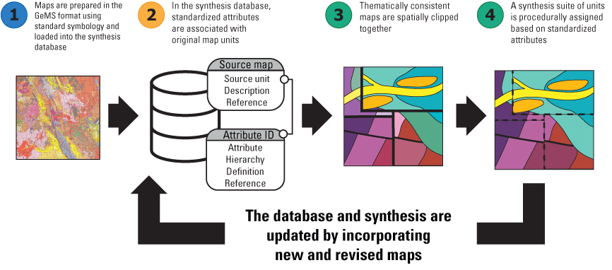
Schematic of the workflow used to populate and update the National Geologic Map Synthesis database. In step 1, maps are prepared and loaded into the database. Relationships in step 2 are exemplary, actual table and attribute names are more thoroughly described in figures 6–9. In step 3, thick lines represent the borders between different component maps. Step 4 illustrates the synthesis of geology through the application of a standard color palette across input maps. Coloring of numbers corresponds to that used to illustrate the structure of the synthesis database shown in figures 5–9. GeMS, Geologic Map Schema; ID, identification.
To apply this synthesis routine in an efficient, reproducible way, we introduce a flexible system that parses source units into a generalized framework based on standardized attributes of source maps units. This system uses a hierarchical system of queries, inspired by semantic triples, that are documented in a table that describes the map units. For example, querying for the terms “age,” “inherits from,” and “Mesozoic” will select all units with an age of Mesozoic or within the Mesozoic and pass this selection to any descendants of this record. This enables the production of many potential derivative maps that “read” like traditional maps, allows synthesized units to be easily adjusted as necessary, and allows for near-instantaneous incorporation of new maps into the existing synthesis.
The procedural intake of maps and application of synthesized map units allows the map synthesis process to be separated from the laborious work of interpreting new geology, forgoing a traditional seamless compilation map in exchange for rapid delivery and ease of updating. This approach places units into a new overarching geologic framework based on the content of the source maps while preserving the original interpretations of the source map authors, giving contributors control over how their regions are portrayed. Rather than being reinterpreted by the compiler, map boundaries can be harmonized by groups of experts working out the relevant issues and incorporating results into new or revised geologic maps that can easily be brought into the synthesis database.
Because the GeMS standard is now mandatory for all NCGMP geologic maps, the synthesis database is built on GeMS as an input, output, and internal format. As GeMS allows for some variability in how the same map content can be encoded, we apply additional standardization to input GeMS geodatabases prior to bringing those maps into the synthesis database. This process is described fully in the “Preparing Component GeMS Databases” section but primarily involves the application of a consistent glossary and symbology.
The synthesis database is built to host multiple scales of maps per the call for “detailed national and continental-resolution” information (U.S. Congress, House Appropriations Committee, 2020, p. 48–49). As these terms were not defined in the original authorizing language, we consider “continental” resolution to be small-scale maps such as the Reed and others (2005) and King and others (1974) maps; “national” resolution to be the scale of existing State geologic maps, ranging from 1:100,000 to 1:1,000,000 (most commonly 1:500,000); and “detailed” resolution to be maps in the 1,24:000 to 1:100,000 scale range. For this report, we first focus on bringing together State geologic maps and regional USGS maps in the “national” scale range (that is, approximately 1:500,000 scale), but the database and processes described here have been built to accommodate higher- or lower-resolution maps in the future.
Motivations for Multiple Layers
A national compilation that “brings together” geologic maps produced throughout the United States must reconcile fundamental differences in geologic mapping across the United States (fig. 2). In the glaciated regions of the Central and Northeastern United States, a profound unconformity separates pre-Quaternary (mostly Mesozoic and older) bedrock from overlying Quaternary glacial deposits (fig. 3A). This unconformity has long motivated the production of separate surficial and bedrock geologic maps (fig. 2). In contrast, the Western and Southeastern United States feature much more variable Quaternary geology that is often volcanic and (or) involved in active deformation and may be continuous from the Tertiary to Quaternary (fig. 3B); this typically results in “Earth’s surface” geologic maps portraying everything from Archean to Holocene rocks in a single map (fig. 2). In parts of the Central United States, the geology of the buried Precambrian basement has also been mapped or inferred separately using limited bedrock outcrops and borehole and geophysical data (fig. 3C).
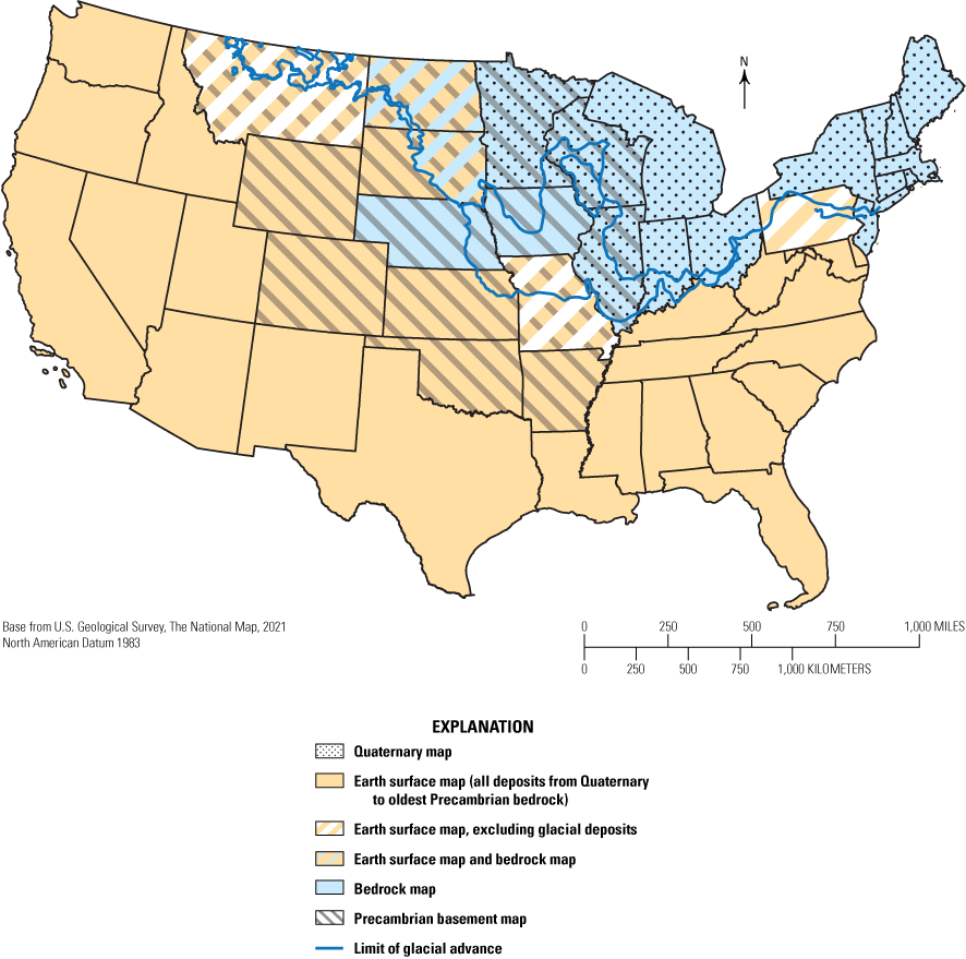
Map compiled from different geologic maps of the United States showing the different styles of geologic mapping produced at statewide and regional scales. Inventory of map styles is derived from maps present and referenced in the map synthesis database. The term “Quaternary map” refers to the primary geology depicted, but, in some cases, the maps are termed “surficial maps” and may contain some non-Quaternary units. The limit of the Laurentide ice sheet from Reed and others (2005) is shown for reference.
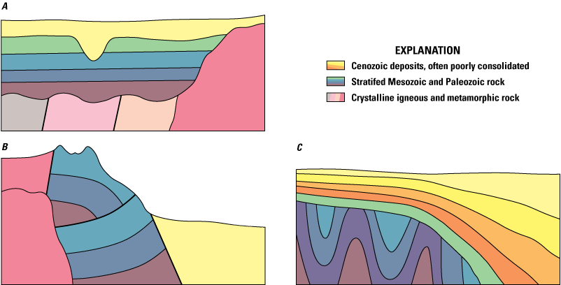
Schematics of regional cross sections of areas in the United States highlighting the relationship between geologic structure and styles of geologic mapping. A, Schematic representing glaciated regions of the United States where major regional unconformities separate Precambrian crystalline basement from Mesozoic and Paleozoic bedrock and Quaternary glacial deposits, all frequently within reach of outcrop and boreholes and amenable to mapping separately. B, Schematic representing tectonic and volcanically active areas in the Western and Southeastern United States with extreme lateral variability in rock types, crystalline rocks at the surface, and thick Cenozoic basin fill with no subsurface constraints, which are usually mapped as a single layer or only as surficial deposits. C, Schematic representing the coastal plains of the Atlantic and Gulf Coasts where the Quaternary is continuous into the Neogene and thickens toward the coast, and underlying basement rocks are known only from borehole intercepts and not mapped separately on geologic maps.
Previous national geologic maps have addressed differences in regional geology and associated mapping styles with purposefully inconsistent depictions of U.S. geology, most easily visualized through the different extents of Quaternary geology shown on previous national maps (fig. 4). The Geologic Map of the United States (fig. 4A, King and others, 1974) and The Geologic Map of North America (fig. 4B, Reed and others, 2005) both chose to emphasize the longer pre-Quaternary geologic record, omitting the extensive Quaternary deposits resulting from continental glaciations with only a line depicting the glacial extent. Similarly, The SGMC (Horton and others, 2017) compiled available bedrock maps, but, because those maps do not cover the entire conterminous United States, the compiled map has abrupt truncations of Quaternary geology along State lines or, in the case of South Dakota, within a State (fig. 4C). The acknowledgment that “Pleistocene deposits can be sacrificed without regret, even though [glacial deposits] attain thicknesses of many hundreds of feet” (King and Beikman, 1974, p. 34) reflects the reality that a single interpretive map is subject to the preferences of the compilers and may deviate from regional priorities because, as King put it, “in the end, the compiler is KING [sic]” (Reed, 2005, p. 7).
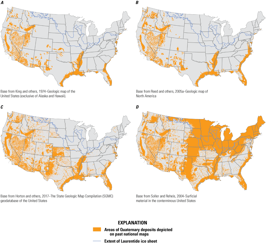
Maps highlighting depictions of Quaternary geology in recent geologic maps of national scope. A, “The Geologic Map of the United States” by King and others (1974). B, “The Geological Map of North America” by Reed and others (2005). C, “The State Geologic Map” by Horton and others (2017). D, “The Surficial Materials in the Conterminous U.S. Map” by Soller and Reheis (2004). Digital datasets provided by A, Schruben and other (1994); B and D, by Soller and others (2009); and C, by Horton and others (2017).The King and others (1974), Reed and others (2005), and Soller and Reheis (2004) geologic maps depict glacial limits, but figure 4 uses the limits of the Laurentide ice sheet from Reed and others (2005) and Garrity and Soller (2009) as a comparable reference in each map. Unlike the other, more general geologic maps in panels A–C, the map in panel D emphasizes Quaternary unconsolidated deposits and residual materials.
Given the goal to bring together geologic data produced by Federal and State partners, we embrace these contrasting styles of geologic mapping to produce four thematic synthesis map layers:
-
1. A Quaternary geologic map layer—The Quaternary map layer emphasizes geologic units that were deposited during the Quaternary, inclusive of units spanning the Neogene–Quaternary (Barrette and others, 2025). Although the base of the Quaternary was recently revised to be significantly older, absolute chronologies directly tied to map units that conflict with original age interpretations are rare1 . Geology in the Quaternary map is derived from dedicated Quaternary geologic maps where they exist and from Earth’s surface style maps elsewhere. Where present, units older than Quaternary are characterized with a few simple attributes based on lithology.
-
2. An Earth’s surface geologic map layer—This map depicts all geology exposed at Earth’s surface, ignoring soil or minor colluvial deposits (Colgan and others, 2025). The Western and Southeastern United States is already mapped this way (fig. 2), but Quaternary and pre-Quaternary (bedrock) geology is shown on separate maps in glaciated lands in the Central and Northeastern United States. These maps are merged into a single layer by using Quaternary geology to mask and crop underlying pre-Quaternary geology, then the result is appended to remaining Earth surface maps. For consistency with single-layer Earth surface maps, we replace bedrock, residuum, and colluvium shown on Quaternary maps with bedrock geology from dedicated bedrock maps during this process.
-
3. A pre-Quaternary geologic map layer—The pre-Quaternary map layer emphasizes geology older than Quaternary, similar to previous national geologic maps and the SGMC (Platt and others, 2025). The layer is assembled from both pre-Quaternary bedrock maps in the glaciated regions of the midcontinent and northeast, and from Earth’s surface maps elsewhere. The pre-Quaternary layer includes Precambrian geology, but not where it is buried by younger rocks and exclusively depicted on dedicated Precambrian geologic maps. Where present, Quaternary cover is categorized as a generic cover unit. This map corresponds to either the Earth’s surface where no Quaternary geology is present or the subsurface base of Quaternary deposits.
-
4. A Precambrian geologic map layer—The Precambrian map layer emphasizes Precambrian geology at both the Earth’s surface and at the buried top of Precambrian surface, generally, though not entirely, corresponding to what is termed “basement” in the Central United States (Hirtz and others, 2025). This layer is composited from Precambrian outcrops on all types of maps, inclusive of deposits that may range into the Paleozoic.
When working with vintage maps, we ensure map unit ages are not in conflict with any reported dates in the map unit descriptions. Of around 10,000 descriptions in the first version of the synthesis database, about 500 contained text of numbers followed by age signifiers (for example, Ma or Myr for one million years, ka or Kyr for one thousand years), only about one-half of which were from the Phanerozoic and only 9 of these reported ages were between the previous and revised lower boundary of the base of the Quaternary. Fewer unit descriptions conflicted with the reported age. Of the 36 unit descriptions that included text of ages and had a maximum reported age of Quaternary, none required revision. However, 3 of the 19 unit descriptions that included text of ages and had minimum ages of Paleogene required revision.
In addition to maintaining consistency with regional geologic mapping styles, this multilayered geologic map approach provides two distinct benefits. First, in contrast to some previous national maps (for example, fig. 4), this mapping approach explicitly indicates the geology that is depicted in each map layer and reveals important subsurface relationships. Second, these layers are defined by 2D surfaces of geologic significance (for example, the present Earth surface or the top of pre-Quaternary units) that facilitate integration with 3D models (Shelton and others, 2022).
The synthesis database provides four geologic map layers, and the primary maps and associated unit descriptions of this geology are housed within the same database and described with the same vocabularies. The four geologic map layers are assembled from different subsets of the source map data to produce a topologically consistent product that functions like a traditional digital GeMS geologic map, as described in the “Data Structure” section. Moreover, the definition and identification of these layers within the synthesis database are not hard coded; map data for each layer are identified through relationships to a table that names and defines each layer. If the need for different map layers is identified by community input or new mapping efforts, the different map layers can be accommodated without changing the underlying data structure.
Data Structure
This report makes repeated reference to the USGS GeMS. Readers who are unfamiliar with the GeMS format should refer to the defining publication published by NCGMP (2020) for more detail, as this report only provides an abbreviated summary. GeMS organizes the content of a digital geologic map produced for use in a geographic information system into a set of spatial and nonspatial tables. The primary nonspatial tables in the GeMS format are (1) a “DescriptionOfMapUnits” table that provides names and descriptions of the units used in the map, (2) a “GeoMaterialDict” that provides a list of standard geologic materials associated with the map unit, (3) a “DataSources” table that provides references used by the map, and (4) a “Glossary” table that defines terms used throughout the data. Spatial tables parse different thematic aspects of the maps based on the types of geologic content and the type of vector data needed to represent that geologic content (for example, points, lines, or polygons). Spatial tables include things such as: (1) “MapUnitPolygons” table of polygons that stores the extent of map units, (2) “ContactsAndFaults” that define the nature of boundaries between “MapUnitPolygons,” (3) “GeologicLines” that store linear features describing a map unit, (4) “OrientationPoints” that describe point measurements of planar or linear orientations of geologic features (for example, bedding planes, paleocurrents, foliations, or lineations), and many more. In general, the standard is defined by explicit, verbose table and field names to capture all the content of a traditional map publication.
The GeMS standard is designed with some principles from relational database management; for example, a “MapUnit” column relates spatial data that identify the location of geologic units to the descriptions in the “DescriptionOfMapUnits” table. Similarly, all records throughout the data package are related to a record in the “DataSources” table. To package all tables together, maps produced for the GeMS standard are typically stored in Esri file geodatabases (extension .gdb) or the Geopackage (extension .gpkg) format.
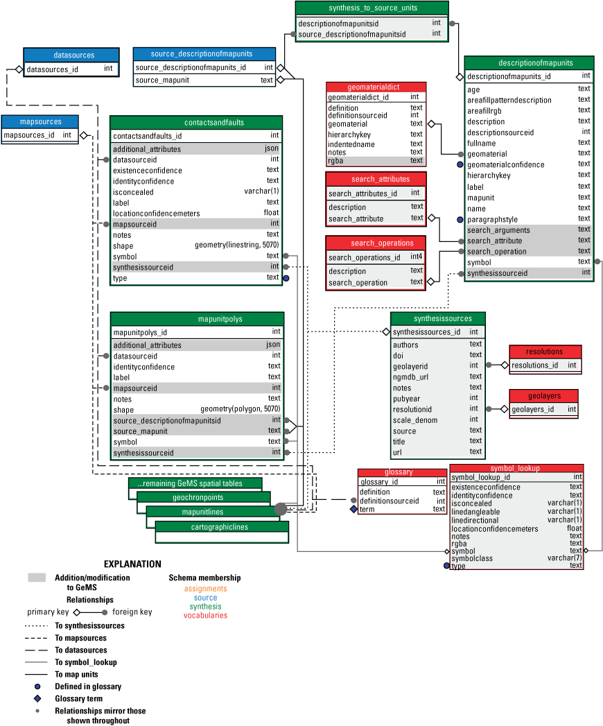
The geologic map synthesis database is structured around four core elements, and the data are organized as collections of tables referred to as “schema” (an organizing framework available in some relational database platforms). Our goal is to present a database that can be read and viewed like a traditional map, but which also preserves the original source map content. We have therefore designed a relational database that allows users to navigate the synthesis map as they would any other GeMS map while retaining the ability to view and query the original interpretations. In describing database elements, we present schemas in bold and italicized text, tables in bold text, and fields in italicized text. Lowercase names are used throughout for database cross-compatibility. The four core elements, illustrated in figure 5, are:
-
1. The synthesis schema houses synthesized map content containing the layers that resemble a traditional national geologic map.
-
2. The source schema is the primary destination for GeMS maps ingested into the synthesis database and preserves the totality of source geologic map data. It serves as an archive of the original maps used in the synthesis as its tables are not altered after they are initially populated.
-
3. The vocabularies schema houses relatively static standard vocabularies used for characterizing map attributes.
-
4. The assignments schema houses tables that link properties from the vocabularies schema to map units in source. As the name suggests, tables in this schema are populated only after the tables are first populated in source.
Flow chart showing a generalized summary of data flow and entity relationship diagram for the synthesis database, with symbolic lines depicting the process of extraction of individual maps and synthesis into derived maps. Tables are colored based on their participation in the four primary schemas of the geologic synthesis database. GeMS, Geologic Map Schema; ID, identification.
Where possible, we seek to mirror conventions outlined in GeMS. For example, providing explicit and verbose names for tables and referencing primary keys as <table name>_id and foreign keys as <table name>id, respectively. Here, <table name> is a placeholder for the name of any table. New tables mimic the structure of existing GeMS tables when possible, as shown in the subset of fields shown in table 1 (for a full list of tables and fields in the synthesis database, refer to the CSV file at https://doi.org/10.3133/dr1210). For example, a vocabularysources table provides references for terms defined in the vocabularies schema and is modeled after the GeMS datasources table. Standard lists of structured scientific terms are given the suffix “dict” and are modeled after the GeMS geomaterialdict. We describe each schema in more detail in the “Source,” “Vocabularies,” “Assignments,” and “Synthesis” sections.
In the description that follows, the term “database” is used to describe three different things: (1) a general concept, (2) the data format of geologic maps contributed to the synthesis database, and (3) the synthesis database described in this report (Johnstone and others, 2025). We attempt to distinguish these by referring to the published geologic maps that populate this product as “input geodatabases” or “input GeMS geodatabases,” where the prefix “geo” just denotes a database with spatial content. In contrast, we describe the product described by this publication as “the synthesis database.” When discussing field names in the GeMS schema and equivalent field names in this synthesis database, we describe GeMS fields in their native mixed case (for example, MapUnit), whereas we use exclusively lowercase fields for the equivalent field names in this synthesis database (for example, mapunit). We further illustrate some of the database functionality with some example queries provided in appendix 1.
Table 1.
Example of database definitions for a subset of tables and fields emblematic of the broader database structure.[The "agedict" and "age" tables are extended from the Geologic Map Schema (GeMS) standard and are isolated from contributed data in different database schemas. For full table definitions, refer to https://doi.org/10.3133/dr1210. --, not applicable]
Source
The source schema contains all the original data from the published maps that were used to build the output map layers. This schema is structured according to the GeMS standard with some minor additions and changes to enable functionality when cataloging many maps. We standardize the GeMS glossary and geomaterialdict tables and relocate them to the vocabularies schema, as described in the “Vocabularies” section of this report. We also add a mapsources table that defines the references for each ingested map. All other tables within source are extended with an integer mapsourceid field that is a foreign key to mapsources. This mapsourceid foreign key enables easy selection of records derived from a particular map, including viewing the map in its entirety. It also enables a “cascade delete” in structured query language that removes a mapsource record and all referential records prior to inserting an updated map. The mapsources table mimics the datasources table, with additional fields that parse the reference (fig. 6).
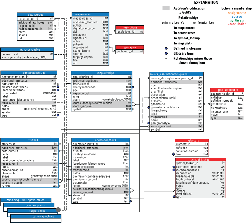
Entity relationship diagram for the source schema that shows tables, relationships between tables, field names, and field types. As the source schema largely mimics Geologic Map Schema (GeMS), we specifically highlight those fields and tables that extend that standard here. Tables are colored based on their participation in the four primary schemas of the geologic synthesis database, as shown in figure 5. For readability, we do not include all the spatial tables from the source schema but show common tables that depict the general structure, which are schematically identical to the GeMS standard except for the additions depicted here. Important relationships to tables outside of the source schema are also shown, but the full detail of those related tables is shown in the respective diagrams for those figures (figs. 7, 8, 9). Similarly, we only show a subset of tables defined by the GeMS standard, which are all extended in the same way as those depicted here.
In GeMS, the MapUnit field functions as the primary and foreign keys between spatial data and the table describing geologic map units. To preserve this relationship in the synthesized maps while explicitly referencing source interpretations, we recast the GeMS “DescriptionOfMapUnits” table as the source_descriptionofmapunits table and rename the “MapUnit” primary/foreign key fields to source_mapunit. We retain the usage of mapunit fields in the synthesis schema, but only for the synthesized map units that are intended to be the legible cartographic representation of the map as a whole, as described in the “Synthesis” section of this report. Individual input GeMS geodatabases have unique “MapUnit” keys, but these keys are not unique among multiple input GeMS geodatabases. We adopt a similar strategy to the SGMC (Horton and others, 2017). That is, each source_mapunit record is made unique by prepending the primary key defined by that record’s entry in the mapsources table. For example, map unit “ T v” from mapsourceid 31 is assigned a source_mapunit of “31 | T v.” This provides a human-readable primary/foreign key in the spirit of the GeMS MapUnit field. In addition, we maintain an integer primary/foreign key to the source_descriptionofmapunits table by using a source_descriptionofmapunits_id primary key in that table and a source_descriptionofmapunitsid foreign key in all GeMS tables that natively contain a GeMS MapUnit field. This additional integer primary/foreign key, despite being functionally redundant with source_mapunit, may be more efficient for some database operations and complements the <tablename>_id structure used elsewhere. Moreover, we expect that users of geologic maps expect map unit conventions when working with and reading geologic maps, but database practitioners will be more familiar with the <tablename>_id syntax.
All tables in this schema are also given an additional_attributes field that is a JavaScript Object Notation (JSON) data type. The additional_attributes field accommodates any feature-level content in source maps that is not defined in the GeMS standard. This field allows for the preservation of content from source datasets without having to prescribe what the field names defining that content must be. This field is populated as part of loading an input map; any fields in an input map table that do not have a corresponding field in the equivalent tables of the synthesis database are stripped from the core table and placed into the additional_attributes field. Each record then has a key, which is the value pair for the field name and field value of that record. For example, a map that created an additional field in its GeMS database to track Quaternary faulting might have a record in the additional_attributes table of “{“AgeOfRecentFaulting”: “latest Pleistocene”}.” The exception to the additional_attributes field is the mapsources table, which instead gets an additional_features JSON field to summarize additional spatial and nonspatial tables present in the source database that are not specified by the GeMS standard. The JSON record for these rows will have keys that are the names of additional tables (spatial or nonspatial) not specified by the GeMS standard and a value that is a list of the columns within those tables. This is used to track any emerging trends in additional GeMS content being produced and to summarize for users what other information may be present in the source map.
Finally, the datasources table is given an additional multidatasourceids field that is an array of self-referencing integer keys that point to other records in the datasources table. This table is used to capture entries from input GeMS geodatabases that utilize delimited data sources (for example, Turner and others, 2022) while maintaining referential integrity between the datasources table and records throughout the synthesis database.
Vocabularies
Tables under vocabularies define terms used throughout the synthesis database (fig. 7). This includes the standard GeMS glossary table for unstructured terms and definitions and the structured geomaterialdict vocabulary specified by GeMS. The vocabularies schema contains a vocabularysources table for references made throughout all other tables in the schema, related through integer primary and foreign keys vocabularysources_id and vocabularysourcesid, respectively. This schema also provides a reference for symbol fields used for the symbolization of vector data throughout the synthesis database, symbol_lookup, for which we rely on the FGDC standard (USGS, 2006). This schema contains other tables defining scientific vocabularies that inherit, and in places extend, the structure of the GeMS geomaterialdict table used to assign source map units to searchable attributes. We draw these vocabularies primarily from the Commission for Geoscience Information (CGI) vocabularies register (CGI, 2020). Currently there are vocabularies that describe the confidence with which standard attributes are assigned to source map units (confidencedict), the International Commission on Stratigraphy timescale (agedict; Cohen and others, 2024), the lithology table from the SGMC (lithologydict, Horton and others, 2017), and a table describing the prevalence of an attribute within a unit derived largely from CGI’s “proportion term” (proportiondict). Future versions of this product may extend this collection of vocabularies based on demand for a particular vocabulary and the ability to relate terms in that vocabulary to source map descriptions without requiring interpretation and manual assignment on a unit-by-unit basis.
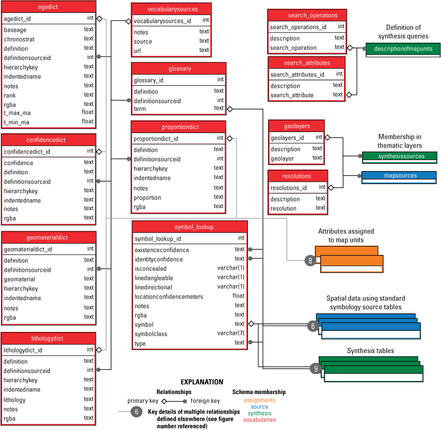
Entity relationship diagram for the vocabularies schema showing tables, relationships between tables, and data types. Tables are colored based on their participation in the four primary schemas of the geologic synthesis database, as shown in figure 5. Important relationships to tables outside of the vocabularies schema are also shown, but full detail of related tables is shown in figures 6, 8, and 9.
Structured vocabularies stored in <vocabularyname>dict tables share a common base structure inherited from the GeMS geomaterialdict table. Here <vocabularyname> references one of the standard vocabularies previously described, such as the “confidence” vocabulary in the confidencedict table. These tables all have <vocabularyname>dict_id primary keys, a hierarchykey field to define the taxonomy of that vocabulary, a definition field that defines that record, a vocabularysourceid foreign key to the vocabularysources table, the term itself listed in the <vocabularyname> field, and an indentedname field derived from <vocabularyname> that provides a more human-readable representation of the hierarchy key and name. An rgba field defines the comma-separated red, green, blue, and alpha values defining a unique color for each record that can help users visualize attributes. Additional fields are added to tables as needed; for example, a rank and t_min_ma field is added to the agedict table to describe the formal stratigraphic rank and minimum age of a chronostratigraphic interval.
Aggregation of source map units into a subset of synthesis map units is done procedurally with a series of queries. In adherence with FAIR principles (findability, accessibility, interoperability, and reusability; Wilkinson and others, 2016), the synthesis needs to be reproducible, so we define and store the queries used for synthesis in the synthesis database. These queries are based on the searched attributes of source maps and what constitutes a match between a source map and an attribute of interest. The names of the searchable attributes and the search operations are defined by the search_attributes and search_operations tables in the vocabularies schema. Each table contains three fields: an integer primary key (<tablename>_id), a text definition (description), and the name of the attribute or operation (search_attribute or search_operation). A value being searched for also guides each query, but those search values are defined by the corresponding vocabularies.
We envision opportunities to extend these vocabularies and the assigned connections to map units, described in the “Assignments” section, in subsequent versions of this synthesis database. Possible inclusions include other concepts defined within GeoSciML and the CGI vocabularies (CGI, 2020), standard geologic names referenced to the National Geologic Map Database Geologic Names Lexicon (“Geolex”; Stamm and others, 2000; https://ngmdb.usgs.gov/Geolex/), references to a unified stratigraphy akin to the approach of Macrostrat (Peters and others, 2018; Quinn and others, 2024), and the geologic provinces concept of the SigMa-GeMS extension (Turner and others, 2022).
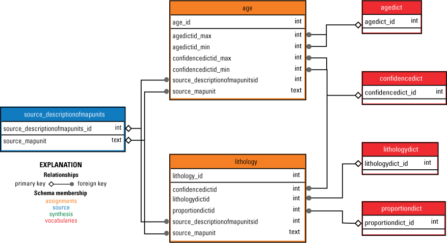
Assignments
The assignments schema contains tables that link the source.source_descriptionofmapunits table to standard vocabularies. Each table in this schema is merely a set of pointers in two directions containing source_mapunit and source_descriptionofmapunitsid foreign key values to the source_descriptionofmapunits table and additional foreign key references to entities in the vocabularies schema. Rather than extending the tables within GeMS with additional pointers to vocabularies, independent tables for linking searchable terms separate source data and the classifications made during synthesis and enable more flexibility in how these attributes are related to source data. This flexibility, illustrated in figure 8, includes associating as many attributes from a particular vocabulary as may be necessary to describe the contents of a source_mapunit (for example, associating a map unit with more than one lithology).
Entity relationship diagram for the assignments schema. Tables are colored based on their participation in the four primary schemas of the geologic synthesis database, as shown in figure 5. Important relationships to tables outside of the assignments schema are also shown, but full detail of related tables is shown in figures 6, 7, and 9.
The age table has a one-to-one relationship with the source.source_descriptionofmapunits table. This table allows for standardized assignments of bounding ages described by the source.source_descriptionofmapunits table’s age field based on chronostratigraphic ages. Minimum and maximum chronostratigraphic age bounds are defined by foreign keys to the vocabularies.agedict table. Confidence values are related to each assignment of a chronostratigraphic age by a foreign key to the vocabularies.confidencedict table. This table is populated by automated parsing of the values of the age field in the source.source_descriptionofmapunits table, as described more completely in the “Populating Assigned Map Attributes” section of this report.
The lithology table has a many-to-one relationship with the source.source_descriptionofmapunits table because one map unit may contain multiple lithologies. Each record in this table has a reference to the vocabularies.lithologydict table, a proportion qualifier referencing the vocabularies.proportiondict table, and a confidence value referencing the vocabularies.confidencedict table. This table is populated by automated parsing of the content of the name and description fields in the source.source_descriptionofmapunits table, as described more completely in the “Populating Assigned Map Attributes” section of this report.
Synthesis
The synthesis schema mimics the structure of the source schema; however, each synthesis schema table also contains a reference to a synthesissources table (fig. 9). The synthesissources table mimics the structure of source.mapsources but instead defines the reference for the current version of the synthesis map layers. The synthesissources table includes geolayerid and resolutionid foreign keys to the geolayers and resolutions tables of the vocabularies schema. Within the synthesis database, all synthesis map layers are stored in the same tables, and these two foreign keys relate each record to its corresponding resolution (for example “national” and “continental” from the motivating language of House Report 116-100 [U.S. Congress, House Appropriations Committee, 2020]) and thematic layer (for example, “Quaternary,” “Earth’s surface”) through reference to the resolutions and geolayers tables in the vocabularies schema. As with tables in the source schema, this creates database tables that violate GeMS compliance because of the topologic errors inherent with multiple overlapping maps. However, layers with valid topology can easily be derived with simple queries to select records matching a single thematic map layer and resolution. With this strategy, the underlying database schema does not need to change to accommodate changes in the resolutions or thematic layers present. Each GeMS-like table in the synthesis schema also includes a source_<tablename>id foreign key that is a reference to the corresponding table in the source schema. Additionally, we export stand-alone GeMS geodatabases with a subset of the full database content for each synthesis map layer for users wanting to work with a single-layer geologic map in the expected format.
Entity relationship diagram for a subset of the synthesis schema and key relationships to other schemas. Tables are colored based on their participation in the four primary schemas of the geologic synthesis database, as shown in figure 5. As the synthesis schema largely mimics Geologic Map Schema (GeMS), we specifically highlight those fields and tables that extend that standard here. For readability, we do not include all the spatial tables from the synthesis schema but instead show only common tables that depict the general structure, which are schematically like those in source and defined by the GeMS standard. Important relationships to tables outside of the synthesis schema are also shown, but full detail of related tables is shown in figures 6, 7, and 8.
The similarity between the synthesis and source schemas ends with the table that describes map units. As this is the starting point for interacting with and reading the synthesized map layers, the descriptions of map units for the synthesis schema are stored in a conventionally named descriptionofmapunits table with a mapunit field; however, there is no table for source map unit descriptions because that information is already stored in the source schema. This descriptionofmapunits table contains three additional fields that dictate how source map units are aggregated into synthesis map units: search_attribute, search_operation, and search_argument. These three fields, inspired by the subject, object, and predicate structure of “Resource Description Format” or “semantic” triples (World Wide Web Consortium, 2004), guide queries that are used to select source map units (source_mapunit) and assign them to synthesis map units (mapunit). We describe this algorithm more in the “Assigning Synthesis Map Units” section of this report. The search_attribute field contains the name of one of the standard attributes associated with source map units (for example, geomaterial for the geomaterialdict, or chronostrat for the agedict) and is a foreign key to the search_attributes table of the vocabularies schema, which also provides a definition. The search_operation term is a foreign key to the search_operations table of the vocabularies schema. These search operations define how source map unit attributes are related to a particular term. For example, a term can exactly match the attribute, or it could be a descendent of another term in that vocabulary’s taxonomy as specified by the hierarchy key as the term “Holocene” is descended from the term “Quaternary.” The search_argument field contains the argument that is used to drive the query. In general, this will be a term, or set of terms separated by semicolons, from the vocabulary specified by the search_attribute field. For example, to identify glacial sediment based on a geomaterial value in search_attribute the term might be “Glacial till.”
Finally, a synthesis_to_source_units table defines the many-to-many relationship between source map units and the synthesis units of the descriptionofmapunits table. This table has two foreign key columns, descriptionofmapunitsid and source_descriptionofmapunits_id, and is populated procedurally based on the search_ fields in the descriptionofmapunits table. Populating this linking table, rather than assigning a synthesis map unit to all appropriate records in the synthesis schema, allows maintenance of relational integrity, simple and quick updates to the assignment of synthesis units, individual source_mapunits to be used in multiple synthesis layers, and repeated values of mapunit in descriptionofmapunits across different synthesis layers. However, to maintain compliance in synthesis map layer GeMS outputs, the MapUnit foreign key fields of spatial data are populated with the synthesis unit.
Format of Exported Geologic Map Schema-Compliant Derivative Map Layers
From the synthesis database, we export isolated derivative map layers as stand-alone GeMS-compliant map datasets. These do not capture the full database content but are instead designed to function like a traditional GeMS geologic map dataset with minimal additional tables and fields upon the expected GeMS standard. The naming conventions in our exported GeMS geodatabases deviate slightly from GeMS conventions and the synthesis database to avoid conflicts with GeMS compliance tests. In addition to standard GeMS fields and tables, spatial tables with a MapUnit foreign key field (which in these exports relates to the MapUnit primary key in the DescriptionOfMapUnits table) also carry a Source_MapUnit field that contains the original map unit from the published source map. The Source_MapUnit field is a foreign key to the equivalent field in the Source_DescriptionOfMapUnits table, which contains all original map unit descriptions. All spatial tables also get a MapSourceID field, which serves as a foreign key to the existing GeMS DataSources table to preserve original record-level data sources and make querying the contributions of individual publications straightforward. We add a Symbol_Lookup table as a reference for geologic symbols stored in foreign key Symbol fields found in spatial tables, Source_DescriptionOfMapUnits and DescriptionOfMapUnits. Finally, we add a synthesis_to_source_units table that relates source and synthesis map units by using two foreign key fields: Source_DescriptionOfMapUnitsID and DescriptionOfMapUnitsID, as well as fields Source_MapUnit and MapUnit.
Populating the Synthesis Database
The synthesis database is populated by preparing input map geodatabases in the GeMS format, ingesting those into the synthesis database, assigning additional standard attributes, subsetting and compositing source maps into the synthesis map layers, and, finally, assigning compilation map units to the composited data. This process requires many of the vocabulary tables to be populated first; however, some of these tables may be appended iteratively if needed, for example, if new maps introduce new types of symbols.
Populating Vocabulary Tables
We populate tables in the vocabularies schema as needed to capture content in input GeMS geodatabases. Dictionary tables (for example, geomaterialdict) are populated in their totality from published scientific vocabularies, such as those provided by CGI (2020), NCGMP (2020), and Cohen and others (2024), that are expected to be complete depictions of some topical area. Although dictionaries may be amended, these tables are intended to remain stable except for minor necessary changes. The glossary and symbol_lookup tables will be amended as new maps are added that require terms or features not yet defined in the synthesis database. The symbol_lookup table is populated based on published USGS standards (USGS, 2006), with substitutions made where those standards do not include a feature. In the glossary, we attempt to use published definitions from widely recognized sources wherever possible, but the definitions may need to be revised in some cases to be specific to geologic mapping contexts. The vocabularysources table will be amended as new references are needed to define terms used throughout the vocabularies schema.
Preparing Component Geologic Map Schema Databases
Source map contributions to the synthesis database are prepared as GeMS level-3 compliant geodatabases as described in NCGMP (2020). In addition to standard GeMS compliance, we enforce a few minor additional requirements to ensure consistency between source maps.
First, to enable visual presentation consistent with longstanding traditions for printed geologic maps, we apply one main transformation to input data by assigning geologic map line and color symbology as codified in FGDC published standards and recommendations (USGS, 2005, 200635). We do not force USGS-preferred color palettes based on age and rock type on source maps, but instead choose the closest match between the 1,000 standard colors and original colors in the published source maps (USGS, 2006). In practice, many modern maps already utilize the FGDC standard, so enforcing this standard symbology suite on source maps largely amounts to minor semantic changes. Making these changes (1) ensures some consistency in basic content and visual presentation and (2) makes many types of mapped geologic features more discoverable through the structure of FGDC symbol codes (for example, all line and point features describing glacial geology have symbol codes that start with the prefix “13”). This same symbology standard is used on derivative synthesis maps. We achieve additional consistency by ensuring symbol values dictate the values in companion fields like type, existenceconfidence, identityconfidence, and isconcealed as specified in the vocabularies.symbol_lookup table and as implied by the FGDC standard. We deviate from the FGDC symbols standard if an appropriate symbol set does not exist.
Second, to facilitate readability, all geodatabases must match a common glossary. For example, “contact” and “Contact” are not tolerated because of differences in capitalization, and both “internal contact” and “contact (internal)” are standardized as “internal contact.” This issue is generally reconciled through the assignment of standard symbology.
Third, all foreign key references to the datasources table must not be null and are preferably not delimited. This contrasts with GeMS, which allows null descriptionsourceid values for records describing headers that are not map units in the descriptionofmapunits table.
Fourth, all hierarchy keys are checked to be sure they are well-formed using equivalent delimiters. Here, “well-formed” means ensuring that hierarchy keys are not only ordered but increase incrementally within each delimited portion. We believe that a well-structured taxonomy for the map units from individual maps facilitates the comparison of map units between maps; therefore, we encourage as much structure as necessary in the descriptionofmapunits table to create a hierarchy key that robustly reflects the ordering and taxonomy of the source material.
Finally, we prescribe additional consistency on the storage of spatial data. Where appropriate, we enforce a common set of map borders (for example, State or county borders) to ensure adjacent maps do not have overlaps or gaps. Bezier curves and multipart geometries are not allowed, and all content is projected into a standard coordinate reference system (currently North American Datum [NAD] 1983 Contiguous USA Albers, EPSG:5070, however, changes to the coordinate system will not impact the overall process or database structure described in this report). We then update how the content in the GeMS table “ContactsAndFaults” is stored, merging contiguous segments of lines with equivalent attributes into a single line and splitting lines at intersections using a process that is sometimes called “planarizing.” This process does not move any vertices or change any attributes other than the “ID” column; instead, it simply ensures that each line in “ContactsAndFaults” is as long as possible and separates two polygons at most.
Extract, Transform, and Load Procedures for Component Map Databases
New input maps are loaded into the source schema from GeMS level-3 compliant geodatabases using an automated extract, transform, and load (ETL) process. Many of the additional consistency checks described in the “Preparing Component GeMS Databases” section of this report, as well as those that are part of the GeMS standard (NCGMP, 2020), are formally implemented as database constraints. For example, a failure to match the synthesis database glossary, which can be updated as needed, will result in a constraint error during load, the result of attempting to add data that have no matching value in the glossary table. Prior to ingesting a source geodatabase, a record is created in the mapsources table to define the mapsources_id primary key that will be assigned to all elements. The ETL routine tracks errors as it loads database content. If any errors are detected, a summary error report is generated, and all records referencing that map are then removed from the synthesis database so that the issue can be reconciled prior to attempting the ETL process again.
Merging an input geodatabase into the source archive requires updating the primary/foreign keys in the input geodatabase to keys from the synthesis database. For example, the GeMS standard suggests keys of DAS1, DAS2, DAS3, and so on for references listed in the DataSources table. Although these keys are unique within each input GeMS geodatabase, they may be duplicated between input geodatabases. Maintaining referential integrity among keys requires ingesting the GeMS geodatabase contents in a certain order dictated by database dependencies viewed as a graph. The first item in the graph does not reference any other tables, the second does not reference any tables other than the first, and so on. In our input geodatabases, this “topologic ordering” ensures the ETL process accesses tables defining primary keys before tables defining foreign keys.
Ignoring the glossary, which in the synthesis database is shared for legibility across source maps, and the GeoMaterialDict, which is already standardized, the topologic order of a GeMS geodatabase is DataSources, DescriptionOfMapUnits, StationPoints, then all other content in any order. We ingest tables in this order, one record at a time. Except for source_mapunit, which is calculated based on mapsourceid and MapUnit values, we do not insert primary key records because they are autogenerated integers. Instead, we keep a record of the primary key values of the source and what those become in the source archive. For example, a GeMS “DataSources_ID” key value of DAS017 may become datasources_id primary key 137 in source.datasources. When ingesting any subsequent GeMS rows with a foreign key reference to that value, the original value is replaced with its updated equivalent.
GeMS compliance has been expanded to accommodate delimited entries in foreign key datasourceid fields (refer to the discussion in Turner and others, 2022). This allows creators of GeMS databases to cite multiple records in the datasources table for a single feature. For example, a DataSourceID value of “DAS01|DAS02” assigned to a contact signifies that two references were used to create that contact. Although this is human-readable and facilitates some data creation, it breaks the relational integrity that aids database maintenance. To maintain relational integrity and preserve the intent of these maps, we adopt the following approach:
-
• Concatenated values are identified and transformed into the minimum number of unique permutations (for example, “DAS01|DAS02” and “DAS02|DAS01” are treated as equivalent);
-
• Each unique combination of references is assigned a new record in the datasources table;
-
• The new composite record is populated with the text “Combination of multiple data sources” and a list of the corresponding values for the component data sources; and
-
• Finally, the multidatasourceids field is populated as a list of the primary keys to the primary entries in the datasources table.
This strategy is similar to that of Turner and others (2022) in that the multidatasourceids field can be used to relate individual records back to their primary citations. However, we have opted to prioritize the relational integrity to the data sources table over human readability because we assume users will more often follow data to their citation than from citations to data.
Populating Assigned Map Attributes
After a map has been ingested into the synthesis database, it can be assigned standard attributes using tables within the assignments schema. Our goal is to parse source maps into standard attributes that can be easily searched, not to reinterpret or otherwise modify the published map unit descriptions. Full source descriptions of map units are retained for any follow-up studies, and it is our goal to ensure those descriptions are correctly discoverable and to not attempt any revisions. As such, we use automated “language processing” to assign standard attributes despite potential limitations in recognizing nuances and equivalence in terminology relative to a trained geologist. However, our processes are reproducible, consistent, scalable, reasonably accurate, time-saving, and can be improved upon and reapplied in the future as needed. In particular, advancements in natural language processing, including large language models, likely present opportunities to advance our attribute characterization by identifying and extracting key attributes of interest (Qiu and others, 2019) or extracting more nuanced semantic associations or predictions from narrative descriptions (Lawley and others, 2022, 202316).
In the following subsections, we describe specific routines used to populate standard attributes. As natural language processing advances, we anticipate opportunities to improve on the approaches described in the “Assigned Ages” and “Assigned Lithologies” sections.
Assigned Ages
The assignments.age table relates source_mapunit values in the source.source_descriptionofmapunits table to minimum and maximum timescale terms and respective confidence values for each. Refer to the “Data Structure” section of this report for more details. The goal of the assignments.age table is to capture and standardize the bounding chronostratigraphic ranges described narratively in the GeMS age field. For each age field, we first apply a suite of substitute terms to a copy of the string that brings ages into alignment with the International Commission on Stratigraphy timescale. These substitutions take two forms: (1) simple word substitutions such as “upper” being changed to “late”; and (2) crosswalks between North American stage names and the International Commission on Stratigraphy timescale, for example, “Late Miocene” becomes “Messinian to Tortonian.” A full list of substitutions is provided in table 1.1. We then tokenize components of the age field by splitting this string into a list of “tokens” separated by common stop words and characters “,,” “and/or,” “or,” “and,” “-,” “to,” and “through.” For example, “Holocene and upper Pleistocene” becomes the strings “Holocene” and “late Pleistocene.” For each age “token,” we find the closest case-insensitive match to the chronostratigraphic periods listed in the vocabularies.agedict table’s age field, allowing for fuzzy matching. Fuzzy matches are identified with the Python difflib module and allowed up to a similarity score of 0.85 (values may be between 0 and 1). This is a normalized measure of the proportion of matching characters relative to the total number of characters based on the Ratcliff-Obershelp algorithm (Ratcliff and Metzener, 1988). In this matching, we ignore parts of the token bounded by parentheses, assuming these are more local or general terms. We then sort matched tokens by the hierarchy key for the chronostratigraphic period defined in the vocabularies.agedict table and take the first and last tokens as the minimum and maximum or, in the case of a single token, take this as both the minimum and maximum. Tokens containing a question mark receive a confidence value of “questionable;” otherwise, tokens are given a confidence value of “certain.” Confidence values are identified by foreign key relationships to the vocabularies.confidencedict table.
Assigned Lithologies
For each source_mapunit in source.source_descriptionofmapunits, there are potentially many relevant standard lithologies. Using assignments.lithology, we assign one or more lithologies to each original source_mapunit by matching the name and description fields to terms in our vocabularies.lithologydict table. Each lithology assignment is further associated with a confidence and relative proportion through relationships to the vocabularies.proportiondict and vocabularies.confidencedict tables. Refer to the “Data Structure” section of this report for more details. For each row in the source.source_descriptionofmapunits table, we tokenize contents from the name and description fields using the Python Natural Language Toolkit module (Bird and others, 2009). Each token is then evaluated for matches to lithologies in the vocabularies.lithologydict table using regular expression searches that seek exact matches. Proportions are assigned based on the field a match occurs in and its relative order in that field. Matches to the name field are related to the “most abundant” entry of the vocabularies.proportiondict table. Matches to the description field are related to the “present” entry unless four or more matches have been identified earlier in the field, in which case “minor” is given as the related proportion. All lithology matches are assigned a confidence of “high” as they represent direct matches to words.
Assembly of Synthesis Map Layers
Much of the value of this compilation will come from the ability to readily query integrated content across source maps to generate derivative products. However, providing a visual synthesis of the geology remains useful for reading the map compilation. Here we discuss the process for building the synthesis map layers, which consists of first assembling and compositing the relevant spatial data, then aggregating relevant source map units to a set of synthesis map units. Each of these processes is designed to make the output maps as readable as traditional geologic maps. Compositing spatial data is a way to produce new topologically consistent spatial geometries from existing maps, whereas synthesizing map units aggregates one or more source_mapunit values with a legible number of synthesis mapunit values. Both compositing and synthesizing must be performed with an end product in mind; that is, a map synthesis theme. However, because many source maps already follow some geologic themes, there are scenarios where the compositing step is equivalent to simple copying. This may occur, for example, when the spatial data being ingested into the synthesis database are already topologically consistent according to a desired geologic theme, such as State geologic maps of the geology at Earth’s surface.
Assembling Spatial Data for Synthesis Map Layers
When building the spatial depiction of the synthesis map layers, we do not manually create any new lines but instead rely directly on the unmodified vector content from source maps in the source schema (fig. 10). Because relevant map datasets may have overlapping extents, this requires cropping out portions of some maps in favor of data from others. For example, map 4 in figure 10 cuts out underlying data, as depicted in figure 10H and 10I. Data from source maps are copied from the source schema into the corresponding synthesis map layers, which are cropped prior to insertion to enforce contiguity. When maps already share a boundary and there is no overlapping data (for example, fig. 10D and 10F), no cropping occurs, but the general approach can be described in the following operation:
-
1. Sort all maps of interest in order of increasing priority.
-
2. For each map in sorted order complete the following steps:
-
a. Create a mask by dissolving the polygons of the source map,
-
b. Clip and remove data from the synthesis map layer that overlaps the mask,
-
c. Clip and preserve the relevant spatial data from the source map using the mask created in step (a), and
-
d. Append the data from step (c) to the synthesis map layer.
-
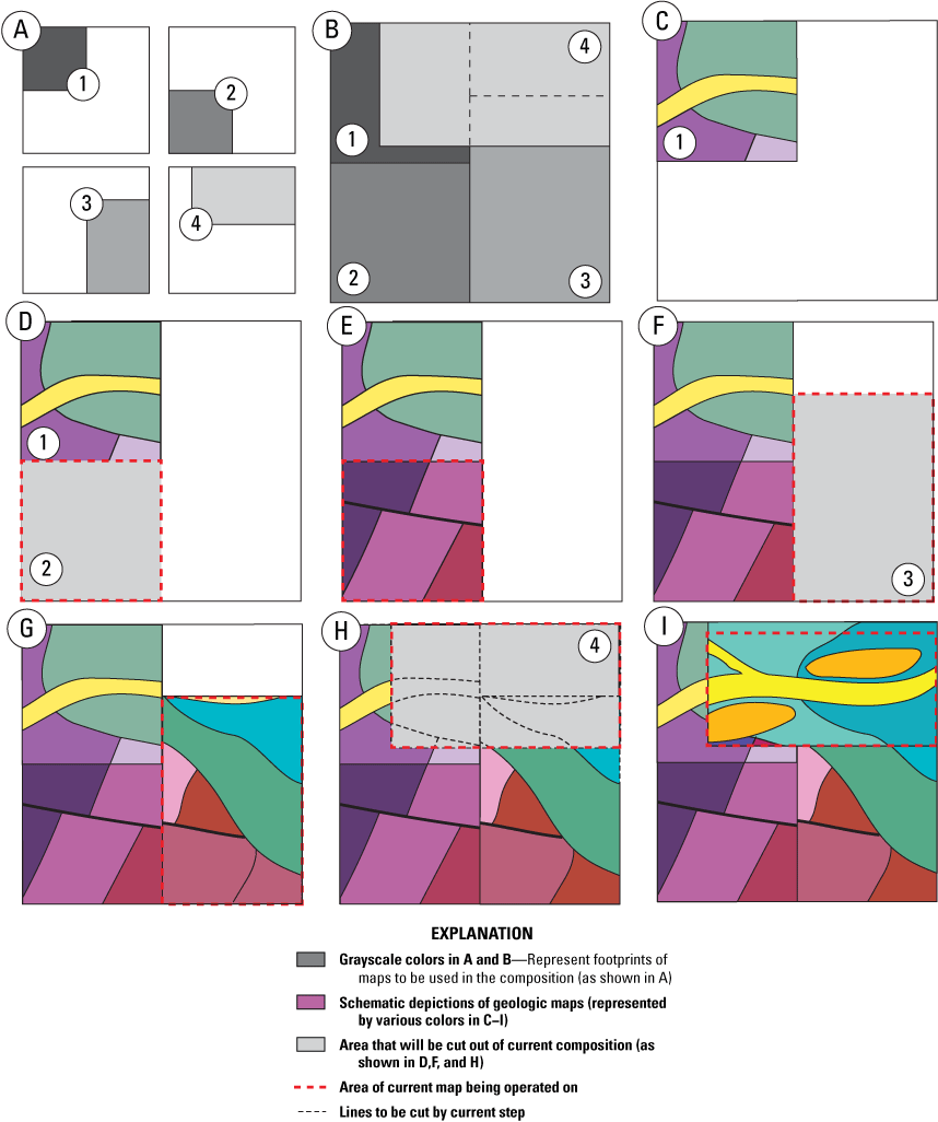
Schematic of the process used for compositing source maps together into a single topologically sound product. Panel A depicts four maps that will be used to fill out a map area. Panel B shows how these maps will be sorted and stacked, with dashed lines indicating map borders (of maps 1–3) that will be below another map (map 4) based on the sorted order. Panel C shows the starting condition, a canvas that only consists of the first map. Panels D–I step through progressively pulling a map from the sorted list, using the extent of that map to cut out underlying mapping (for example, red outline with gray interior in panels D, F, and H), then inserting the map (red outline around colored geology). Although the algorithm is the same, inserting maps 1–3 (for example, panels B and C) requires no clipping and removal of data because those maps are not overlapping.
This compositing process is slightly more complicated for certain maps, for example, compositing bedrock and Quaternary maps to create the Earth’s surface synthesis layer. Rather than selecting all polygons and spatial features of interest in steps 2a and 2b, only a subset of relevant features is selected. For example, to reproduce an “Earth’s surface” map from separate pre-Quaternary and Quaternary maps, we first composite the bedrock maps, then follow the above procedure for only a portion of the polygon units in the Quaternary maps, such as those with a minimum age bound of Quaternary that are not colluvial or residuum units. In practice, this simply amounts to adjusting the priority order appropriately, then amending step 2a to create the mask based on a queryable subset of polygons.
A key part of this process is performing the cutting and deletion of new content in such a way that the GeMS topological relationship between polygons, contacts, and faults is preserved and, more generally, that appropriate geologic features are cropped and inserted. We additionally crop geologic lines and map unit lines. Point data do not need to be cropped, only selectively inserted where appropriate. Overlay polygons are handled on a case-by-case basis depending on whether they correspond to regional phenomena or are unique to an individual map. The features themselves are still preserved and searchable in source.
In assigning the order to maps, we default to ordering by scale and recency of publication and assign the greatest priority to the most recent and detailed maps within a particular range defined for each “resolution.” However, we adjust this default ordering where stakeholder input, such as the recommendations of a State geologic survey or other regional expert, or clear differences in geology exist between otherwise comparable maps. The synthesis database design does not prescribe an ordering for compositing maps; rather, that is detailed in the respective companion data releases for those maps.
Assigning Synthesis Map Units
After spatial data are composited into synthesis map layers, synthesis units can be assigned to all spatial records with a mapunit in GeMS. This is done by populating a crosswalk table relating original map units to synthesis units. Rather than assigning source map units to synthesis map units by hand on a case-by-case basis, we build synthesis map units procedurally based on searchable attributes. This approach has three advantages: (1) it is transparent and reproduceable, (2) it allows for efficient updates as new maps are made available, and (3) it yields comparable legends to past national efforts. The Geologic Map of the United States (King and others, 1974), currently the most detailed seamless depiction of the geology of the conterminous United States, has almost 200 map units. The legend for these map units is depicted as a matrix, rows being a chronostratigraphic timescale and columns being broad categories of where or how rocks formed, such as “continental deposits,” “eugeosyncinal deposits,” and “volcanic rocks.” Only about 20 percent of the map units in the Geologic Map of the United States are assigned based on formal stratigraphic names, and about 16 percent are Permian strata (King and Beikman, 1974). This is, at its core, a procedural assignment of map units, the difference being the authors decided which properties of generalized map units to emphasize, whereas we let the properties derive from the sources directly, for example, from the age and geomaterial fields populated by the source publications. The Geologic Map of North America by Reed and others (2005) relies on a similar strategy; that is, units are largely named based on broad lithologic categories and age. Compared to the years it took the authors of those maps to create and assign that compilation stratigraphy, the approach described in this report can assign thousands of source units to synthesis units within seconds.
The synthesis.descriptionofmapunits table is manually populated as part of the creation of a derivative synthesis map and is used to drive the assignment of source map units to synthesis map units. The records in this table are inserted and iteratively refined by geologists in the process of constructing the derivative synthesis map layers, a target we discuss more at the end of this section. The materials, ages, and descriptions of each synthesis unit are written to be a summary of the totality of source units it represents, based on a summary of the assigned units. Our algorithm for assigning source map units to synthesis map units relies on successively refined queries that are applied according to the taxonomy defined in the hierarchykey field of a synthesis map layer’s synthesis.descriptionofmapunits records. These queries are defined by an additional selection field in the synthesis.descriptionofmapunits table for each synthesis layer and are applied by chaining selections together according to the structure of the hierarchy key. This approach operates recursively, that is, a record in the synthesis layer’s synthesis.descriptionofmapunits table specifies a selection that subsets any existing selection and passes that refined selection to descendants in its hierarchy key. Records with non-null mapunit values apply that map unit to any selected records that are not assigned a mapunit by their descendants. Procedurally, this looks like the following:
-
1. Identify each source map unit used in a synthesis map layer and add these to a list of selectable source map units;
-
2. Initialize a crosswalk table with a row for each source map unit and columns for the source map unit and the corresponding synthesis map unit;
-
3. For each row corresponding to a top-level hierarchy key in the synthesis description of map units (DMU) table in sorted order:
-
a. Use the query logic specified by this row to identify and split the currently selectable source map units into those that do and do not match this query;
-
b. Find all immediate children of the current synthesis hierarchy key;
-
c. For each, if any, children identified in step 3b in sorted order:
-
d. If the synthesis DMU row is a map unit, assign the subset of units identified in step 3a, and not already assigned synthesis map units in recursions in step 3c(i), to this row’s synthesis unit by populating the table created in step 2. If this synthesis DMU row has no map unit, return the matched subset to the selectable pool used by step 3a
-
The process used for assigning synthesis map units to source map units, with a simple conceptual example of a subset of a compilation description of map units table, is shown in figure 11. To demonstrate the concept, we describe synthesis criteria in plain language, but detailed descriptions of these queries are stored in the vocabularies schema. The synthesis map units depicted in figure 11 divide source map units (fig. 11A) into two top-level hierarchies (that are shown): those beginning with 01 corresponding to Quaternary geology and 02 corresponding to Tertiary units (fig. 11B–C). Within the Quaternary, units are then parsed into two additional subcategories: 01.01 selects clastic sedimentary units (fig. 11D) and 01.02 selects igneous rocks. Within the Quaternary, clastic sediments are further parsed into glacial or nonglacial categories (fig. 11D). After attempting all assignments at the lowest possible levels, any units not assigned will return to be assigned to a parent or, if there is no parent map unit, will be passed further down the hierarchy. For example, late Pleistocene fine-grained lake deposits would be identified as Quaternary and as clastic sediments but not as alluvial nor glacial, so these deposits would be assigned to Q u (fig. 11E). With all the children of hierarchy key 01 visited, the algorithm proceeds to hierarchy key 02, first selecting all units in the Tertiary (fig. 11F) and passing this selection to be further divided into sedimentary and igneous units. This process continues until all rows in the synthesis description of map units table have been visited. This does not necessarily assign all source map units, so, to construct a consistent and complete set of synthesized map units, the synthesis units will need to be adjusted (for example, by adding new units or making existing units more general) until no orphan units remain (fig. 11G). In assigning synthesis units, we seek a balance between capturing important geologic distinctions and aggregating the Nation’s geology into a legible number of synthesis units.
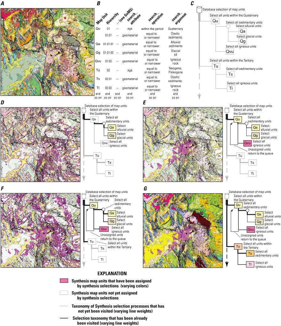
Tabular and schematic graphical representation of the process used for assigning synthesis map units to source map units. A small area centered on the Idaho-Montana-Wyoming border is shown as an example throughout. Panel A depicts the original source map units that will be assigned to synthesis units based on the description of map units table shown in panel B and depicted graphically as a taxonomy in panel C. Panels D, E, F, and G depict points in the recursive iteration through the synthesis unit taxonomy. The saturation of lines and legend labels in the taxonomy indicates the identification of selections (shown by purple highlighted shapes in the map) and application of units (shown by the application of saturated standard colors in the map), respectively. GeMS, Geologic Map Schema; --, Portions of a GeMS description of map units table omitted for brevity.
Target for the Construction of Synthesis Map Units
The map unit synthesis process described in the “Assigning Synthesis Map Units” section will assign source map units to synthesis map units based on the contents of the source maps, including content parsed into tables of the assignments schema. However, there are many potential suites of synthesis map units that could accomplish this for a given set of source units. In general, we seek to produce a visually differentiable suite of units (for example, dozens to around 100 units) that summarize the geology reflected in source map units without over- or under-generalizing any aspect of the geology (that is, balancing the source units across synthesis map units). This system is equally capable of producing more targeted derivative maps based on other geologic map content of interest (for example, examining aggregate potential by producing a derivative of typical grain sizes of young sedimentary deposits); however, we focus here on the national geologic syntheses that are the core derivative products.
We define the “visually differentiable” criteria partly based on the number of units alone because too many units make a map hard to read, and too few communicate limited information. Based on the precedent of published maps, our approximate target is around 50 to 100 map units. The mean number of map units per map in the first version of this synthesis database was 85, and 50 percent of maps had between 34 and 100 units. This is further defined by how the map looks, including both the number of map units as well as how much space they occupy in the map. In our derivative map products, we seek to avoid many very small map units or very few large map units, except when the source geology indicates important transitions across small or large areas.
Given this rough guideline on the number of source map units, we then seek to divide them evenly across synthesis map units. Where a synthesis map unit does not describe very many source units, it will generally be dissolved into a similar unit unless it is desirable to show a particularly unique unit, such as ultramafic rock bodies. Where a synthesis map unit captures a large number of units, or multiple distinct populations of units (for example, based on age or materials), we will seek to split that apart into multiple synthesis units. We adjust the synthesis units repeatedly until a satisfactory result is achieved. Finally, we seek some consistency in synthesis units between the various synthesis map layers so that comparable units are quickly visually associated when looking between different layers.
For the synthesis maps described in this report, we used queries based on the age and geomaterial attributes. With GeMS required on all NCGMP-funded maps, these two fields are guaranteed to be populated in all source maps. Previous national maps have also used units grouped by age and lithology to describe the Nation’s geology (King and others, 1974; Reed and others, 2005). Applying the synthesis strategy described in the “Assigning Synthesis Map Units” section of this report, we begin with broad groupings of age as the highest order taxonomy levels, then split these broad categories based on geomaterials. We divide synthesis units again by age or refine the original age categories, and continue refining as necessary according to the general criteria outlined previously until satisfied with the result.
Summary
This report presents a strategy to integrate maps produced in the Geologic Map Schema (GeMS) National Cooperative Geologic Mapping Program standard into a single synthesis database to derive a suite of synthesized derivative maps. In designing this data structure, we strive to honor the contributions of individual map sources and the regional diversity that exists in mapping style, while facilitating both the construction of visually legible depictions of geology at a national level and the “queryability” of geologic information at the level of individual maps. We have constructed this synthesis database in a way that it is readily updated with revised geologic publications and expandable to include other resolutions and (or) queryable sets of attributes. At its core this process involves (1) the careful assembly of component map datasets to share map borders, a common glossary, and standard symbology into an integrated multi-map database archive; (2) the assignment of standard queryable attributes to map units using well-defined vocabularies; and (3) the subsetting and summary of component maps into a set of synthesis map layers. Through this process, we have provided the first layered depiction of geology at a national scale that captures both the most recent geologic history that dominates the Earth’s surface as well as the longer history recorded in the subsurface.
Beyond providing updates that apply this system to newly published geologic maps, we envision future versions of this product that expand upon this model in three important ways. First, we will look to provide new “resolutions” of geologic mapping that speak to the congressional mandate for “detailed national and continental-resolution geologic information” (U.S. Congress, House Appropriations Committee, 2020, p. 48–49). Second, we will seek to expand upon the standard vocabularies referenced here to provide new pathways for querying the synthesis database, for example, through explicit relationships between named geologic units and Geolex (Stamm and others, 2000; https://ngmdb.usgs.gov/Geolex/) and more robust identification of searchable attributes. Finally, we will look to provide explicit relationships between geology depicted within these map layers and ongoing three-dimensional geologic modeling efforts (Shelton and others, 2022).
References Cited
Barrette, N.C., Johnstone, S.A., Campos, J.-M., Colgan, J.P., and Roe, W.P., 2025, Cooperative National Geologic Map—Quaternary geology: U.S. Geological Survey data release, https://doi.org/10.5066/P16SJAC6.
Barton, K.E., Howell, D.G., and Vigil, J.F., 2003, The North America tapestry of time and terrain: U.S. Geological Survey IMAP, v. 2781, accessed May 7, 2024, at https://doi.org/10.3133/i2781.
Bird, S., Klein, E., and Loper, E., 2009, Natural language processing with Python: Sebastopol, Calif., O’Reilly Media, Inc., 479 p. [Also available at https://www.researchgate.net/publication/220691633_Natural_Language_Processing_with_Python.]
Brock, J.C., Berry, K., Faulds, J., Berg, R., House, K., Marketti, M., McPhee, D., Schmidt, K., Schmitt, J., Soller, D., Spears, D., Thompson, R., Thorleifson, H., and Walsh, G., 2021, Renewing the National Cooperative Geologic Mapping Program as the Nation’s authoritative source for modern geologic knowledge: U.S. Geological Survey Open-File Report 2021-1013, 10 p., accessed November 2, 2021, at https://doi.org/10.3133/ofr20211013.
Childs, O.E., 1985, Correlation of stratigraphic units of North America–COSUNA: AAPG Bulletin, v. 69, no. 2, p. 173–180. [Also available at https://doi.org/10.1306/AD461C73-16F7-11D7-8645000102C1865D.]
Cohen, K.M., Harper, D.A.T., and Gibbard, P.L., 2024, ICS International Chronostratigraphic Chart, version 2024/12: International Commission on Stratigraphy, accessed February 13, 2025, at https://stratigraphy.org/chart#latest-version.
Colgan, J.P., Johnstone, S.A., Campos, J.-M., Platt, B.W., Hirtz, J.A.M., Barrette, N.C., and Roe, W.P., 2025, Cooperative National Geologic Map—Earth’s surface geology: U.S. Geological Survey data release, https://doi.org/10.5066/P146VGVM.
Colman-Sadd, S.P., Ash, J.S., Hayes, J.P., and Nolan, L.W., 1996, Management of geologic map units in a geographic information system: Newfoundland Department of Natural Resources, Geological Survey, Current Research 96–1, p. 227–251. [Also available at https://www.gov.nl.ca/iet/files/mines-geoscience-publications-currentresearch-1996-colman-sadd.pdf.]
Commission for Geoscience Information [CGI], 2020, [Commission for Geoscience Information] CGI vocabularies register: Geoscience Australia web page, accessed January 30, 2024, at https://cgi.vocabs.ga.gov.au/vocab/.
Garrity, C.P., and Soller, D.R., 2009, Database of the Geologic Map of North America—Adapted from the map by J.C. Reed, Jr. and others (2005): U.S. Geological Survey Data Series, v. 424, accessed November 2, 2024, at https://doi.org/10.3133/ds424.
Hirtz, J.A.M., Colgan, J.P., Platt, B.W., Johnstone, S.A., and Roe, W.P., 2025, Cooperative National Geologic Map—Precambrian geology: U.S. Geological Survey data release, https://doi.org/10.5066/P13TSV2J.
Horton, J.D., San Juan, C.A., and Stoeser, D.B., 2017, The State Geologic Map Compilation (SGMC) geodatabase of the conterminous United States (ver. 1.1, August 2017): U.S. Geological Survey Data Series 1052, 46 p., accessed November 28, 2022, at https://doi.org/10.3133/ds1052.
Johnstone, S.A., Colgan, J.P., and Roe, W.P., 2025, Geospatial database for the cooperative national geologic maps: U.S. Geological Survey data release, https://doi.org/10.5066/P1DC4XFG.
King, P.B., and Beikman, H.M., 1974, Explanatory text to accompany the geologic map of the United States: U.S. Geological Survey Professional Paper 901, 40 p., accessed September 15, 2023, at https://doi.org/10.3133/pp901.
King, P.B., Beikman, H.M., and Edmonston, G.J., 1974, Geologic map of the United States (exclusive of Alaska and Hawaii): U.S. Geological Survey, 2 pls. and legend, scale 1:2,500,000, accessed November 28, 2022, at https://doi.org/10.3133/70136641.
Lawley, C.J.M., Gadd, M.G., Parsa, M., Lederer, G.W., Graham, G.E., and Ford, A., 2023, Applications of natural language processing to geoscience text data and prospectivity modeling: Natural Resources Research, v. 32, no. 4, p. 1503–1527, accessed September 15, 2023, at https://doi.org/10.1007/s11053-023-10216-1.
Lawley, C.J.M., Raimondo, S., Chen, T., Brin, L., Zakharov, A., Kur, D., Hui, J., Newton, G., Burgoyne, S.L., and Marquis, G., 2022, Geoscience language models and their intrinsic evaluation: Applied Computing and Geosciences, v. 14, article 100084, 10 p., accessed May 3, 2024, at https://doi.org/10.1016/j.acags.2022.100084.
McGee, W.J., comp., 1884, Map of the United States, exhibiting the present status of knowledge relating to the areal distribution of geologic groups (preliminary compilation), plate 2 in Fifth annual report of the United States Geological Survey to the Secretary of the Interior, 1883–1884: U.S. Geological Survey Annual Report 5, accessed May 7, 2024, at https://doi.org/10.3133/ar5.
National Cooperative Geologic Mapping Program [NCGMP], 2020, GeMS (Geologic Map Schema)—A standard format for the digital publication of geologic maps: U.S. Geological Survey Techniques and Methods 11-B10, 74 p., accessed September 9, 2022, at https://doi.org/10.3133/tm11B10.
Peters, S.E., Husson, J.M., and Czaplewski, J., 2018, Macrostrat—A platform for geological data integration and deep‐time Earth crust research: Geochemistry, Geophysics, Geosystems, v. 19, no. 4, p. 1393–1409, accessed April 30, 2024, at https://doi.org/10.1029/2018GC007467.
Platt, B.W., Colgan, J.P., Hirtz, J.A.M., Johnstone, S.A., Campos, J.-M., and Roe, W.P., 2025, Cooperative National Geologic Map—Pre-Quaternary geology: U.S. Geological Survey data release, https://doi.org/10.5066/P147SGSS.
QiuQ., XieZ., WuL., and LiW., 2019, Geoscience keyphrase extraction algorithm using enhanced word embedding: Expert Systems with Applications, v. 125, p. 157–169, accessed May 3, 2024, at https://doi.org/10.1016/j.eswa.2019.02.001.
Quinn, D.P., Idzikowski, C.R., and Peters, S.E., 2024, Building a multi‐scale, collaborative, and time‐integrated digital crust—The next stage of the Macrostrat data system: Geoscience Data Journal, v. 11, no. 1, p. 11–26, accessed April 30, 2024, at https://doi.org/10.1002/gdj3.189.
Ratcliff, J.W., and Metzener, D.E., 1988, Pattern matching—The Gestalt Approach: Dr. Dobb’s Journal, 46 p., accessed April 20, 2024, at https://www.drdobbs.com/database/pattern-matching-the-gestalt-approach/184407970?pgno=5.
Reed, J.C., Jr., Wheeler, J.O., Tucholke, B.E., Stettner, W.R., and Soller, D.R., 2005, Geologic map of North America—Perspectives and explanation: Boulder, Colo., Geological Society of America, Decade of North American Geology, Continental-Scale Map Series v. 1, pamphlet 28 p., 3 sheets, scale 1:5,000,000, accessed April 30, 2024, at https://doi.org/10.1130/DNAG-CSMS-v1.
Schruben, P.G., Arndt, R.E., and Bawiec, W.J., 1994, Geology of the conterminous United States at 1:2,500,000 scale—A digital representation of the 1974 P.B. King and H.M. Beikman map: U.S. Geological Survey Data Series 11, 1 CD-ROM, accessed November 4, 2024, at https://doi.org/10.3133/ds11rel1.
Shelton, J.L., Andrews, W., Colgan, J.P., Johnstone, S., Soller, D.R., Berg, R., Sweetkind, D.S., Zellman, K.L., Brock, J., and Ritzel, K., 2022, The National Cooperative Geologic Mapping Program’s U.S. GeoFramework Initiative—Delivering a digital database of geologic map information by 2030: U.S. Geological Survey Fact Sheet 2022-3079, 2 p., accessed September 15, 2023, at https://doi.org/10.3133/fs20223079.
Soller, D.R., and Reheis, M.C., 2004, Surficial materials in the conterminous United States: U.S. Geological Survey Open-File Report 2003-275, 1 sheet, scale 1:5,000,000, accessed September 15, 2023, at https://doi.org/10.3133/ofr2003275.
Soller, D.R., Reheis, M.C., Garrity, C.P., and Van Sistine, D.R., 2009, Map database for surficial materials in the conterminous United States: U.S. Geological Survey Data Series 425, 12 p., scale 1:5,000,000, accessed September 15, 2023, at https://doi.org/10.3133/ds425.
Stamm, N.R., Wardlaw, B.R., and Soller, D.R., 2000, GEOLEX—The National Geologic Map Database’s geologic names lexicon in Soller, D.R., ed., Digital mapping techniques ‘00—Workshop proceedings, Lexington, Kentucky, May 17–20, 2000, Proceedings: U.S. Geological Survey Open-File Report 2000–325, p. 31–42, accessed May 4, 2024, at https://doi.org/10.3133/ofr2000325.
Turner, K.J., Workman, J.B., Colgan, J.P., Gilmer, A.K., Berry, M.E., Johnstone, S., Warrell, K.F., Dechesne, M., VanSistine, D.P., Thompson, R.A., Hudson, A.M., Zellman, K.L., Sweetkind, D.S., and Ruleman, C.A., 2022, The Seamless Integrated Geologic Mapping (SIGMa) extension to the Geologic Map Schema (GeMS): U.S. Geological Survey Scientific Investigations Report 2022-5115, 33 p., accessed September 15, 2023, at https://doi.org/10.3133/sir20225115.
U.S. Congress, 1992, National Geologic Mapping Act of 1992—Public Law 102-285: U.S. Government Printing Office, 7 p., accessed September 15, 2023, at https://www.govinfo.gov/content/pkg/STATUTE-106/pdf/STATUTE-106-Pg166.pdf.
U.S. Congress, House Appropriations Committee, 2020, Department of the Interior, Environment, and related agencies appropriations bill, 2020: U.S. Congress, 116th, House Report 116-100, to accompany House bill 3052, 237 p., accessed September 15, 2023, at https://www.congress.gov/congressional-report/116th-congress/house-report/100/1.
U.S. Geological Survey [USGS], 2005, Selection of colors and patterns for geologic maps of the U.S. Geological Survey (ver. 1.0): U.S. Geological Survey Techniques and Methods 11–BI, 19 p., 1 pl. in pocket. [Also available at https://doi.org/10.3133/tm11B1.]
U.S. Geological Survey [USGS], 2006, FGDC digital cartographic standard for geologic map symbolization (PostScript implementation): U.S. Geological Survey Techniques and Methods 11–A2, accessed September 15, 2023, at https://doi.org/10.3133/tm11A2.
Vigil, J.F., Pike, R.J., and Howell, D.G., 2000, A tapestry of time and terrain: U.S. Geological Survey IMAP 2720, 32 p., 1 sheet, scale 1:500,000, accessed May 7, 2024, at https://doi.org/10.3133/i2720.
Wilkinson, M.D., Dumontier, M., Aalbersberg, I.J., Appleton, G., Axton, M., Baak, A., Blomberg, N., Boiten, J.-W., Silva Santos, L.B. da, Bourne, P.E., Bouwman, J., Brookes, A.J., Clark, T., Crosas, M., Dillo, I., Dumon, O., Edmunds, S., Evelo, C.T., Finkers, R., Gonzalez-Beltran, A., Gray, A.J.G., Groth, P., Goble, C., Grethe, J.S., Heringa, J., Hoen, P.A.C’t, Hooft, R., Kuhn, T., Kok, R., Kok, J., Lusher, S.J., Martone, M.E., Mons, A., Packer, A.L., Persson, B., Rocca-Serra, P., Roos, M., Schaik, R. van, Sansone, S.-A., Schultes, E., Sengstag, T., Slater, T., Strawn, G., Swertz, M.A., Thompson, M., Lei, J. van der., Mulligen, E. van, Velterop, J., Waagmeester, A., Wittenburg, P., Wolstencroft, K., Zhao, J., and Mons, B., 2016, The FAIR Guiding Principles for scientific data management and stewardship: Scientific Data, v. 3, no. 1, article 160018, 9 p., accessed April 20, 2024, at https://doi.org/10.1038/sdata.2016.18.
Wilson, F.H., Hults, C.P., Mull, C.G., and Karl, S.M., 2015, Geologic map of Alaska: U.S. Geological Survey Scientific Investigations Map 3340, pamphlet 196 p., 2 sheets, scale 1:1,584,000, accessed November 1, 2024, at https://doi.org/10.3133/sim3340.
World Wide Web Consortium, 2004, RDF/XML syntax specification (Revised): World Wide Web Consortium web page, accessed May 4, 2024, at https://www.w3.org/TR/2004/REC-rdf-syntax-grammar-20040210/.
Appendix 1
Example Queries for Working with the Map Synthesis Database
To illustrate potential uses of the map database starting with simple queries and building complexity, appendix 1 provides examples of queries alongside spatial depictions of the results. In describing database elements, we present schemas in bold and italicized text, tables in bold text, and fields in italicized text.
Selecting Glacial Lines
In the Federal Geographic Data Committee (FGDC) standard (U.S. Geological Survey [USGS], 2006), symbol codes are grouped thematically by period-delimited segments (for example, 01.01.01 for accurately located contacts of certain identity and existence). The codes can be used to select all lines (or point symbols) of a particular family of symbols. In figure 1.1, all geologic lines related to glacial and glaciofluvial features (those that begin with FGDC symbol code13) are selected.
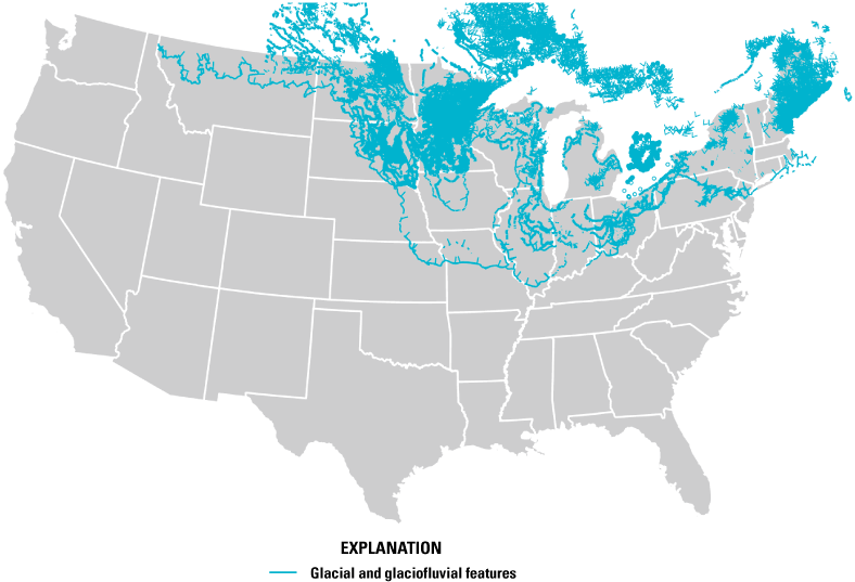
Map of the conterminous United States showing geologic lines related to glacial and glaciofluvial features. Glacial and glaciofluvial features were selected using the following query: SELECT geologiclines_id,symbol,type,mapsourceid, shape FROM source.geologiclines WHERE symbol LIKE '13%'
Selecting the Extent of Pre-Quaternary Map Sources
The mapsourcepolys extent can be joined to the mapsources table, and then the geolayers table, to select the extent of maps of a particular theme. For example, figure 1.2 shows a bedrock map. A shortcut to this query is to use the integer geolayerid in the mapsources table for the map type of interest in the WHERE clause.
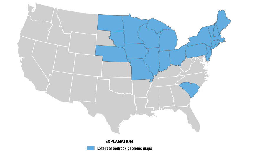
Map of the conterminous United States showing the extent of bedrock. Bedrock was selected using the following query: SELECT sources.mapsources_id, sources.source, polys.shape FROM source.mapsourcepolys AS polys INNER JOIN source.mapsources AS sources ON polys.mapsourceid = sources.mapsources_id LEFT JOIN vocabularies.geolayers AS g ON sources.geolayerid = g.geolayers_id WHERE g.geolayer = 'Bedrock'
Selecting the Faults from Earth Surface Maps
Combining the logic used to create figures 1.1 and 1.2, we can identify all faults (FGDC symbols that start with 02) that are observed in Earth’s surface maps. Figure 1.3 presents a map showing fault lines in the United States.
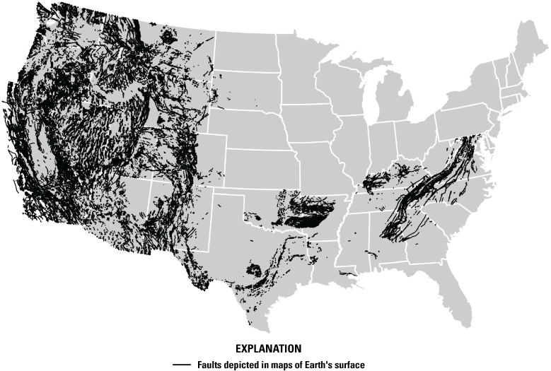
Map of the conterminous United States showing surficial faults. Surface faults were selected using the following query: SELECT contactsandfaults_id,symbol,type,mapsourceid, shape FROM source.contactsandfaults AS caf INNER JOIN source.mapsources AS sources ON (caf.mapsourceid = sources.mapsources_id) INNER JOIN vocabularies.geolayers AS g ON (sources.geolayerid = g.geolayers_id) WHERE g.geolayer = 'Surface' AND caf.symbol LIKE '02%'
Selecting Map Unit Polygons Whose Descriptions Reference a Word
Because full map unit descriptions are preserved and associated with map unit polygons, those descriptions can be searched for keywords or phrases. For example, figure 1.4 shows a simple case-insensitive search for map units whose descriptions mention “graphit,” with the intent of capturing “graphite” or “graphitic.”
Map of the conterminous United States showing graphite or graphitic areas. Graphite or graphitic areas were selected using the following query: SELECT mup.mapsourceid, mup.source_mapunit, mup.symbol, sdmu.description, mup.datasourceid, mup.mapunitpolys_id, mup.shape from ngs.source.mapunitpolys AS mup INNER JOIN source.source_descriptionofmapunits AS sdmu ON (sdmu.source_mapunit = mup.source_mapunit) WHERE description ILIKE '%graphit%'
Selecting Pre-Quaternary Maps and Symbolizing by Age
Here we use parts of the logic from the queries producing figures 1.1–1.4 to select all map unit polygons referencing pre-Quaternary National resolution maps, shortcutting some of the queries with the knowledge that the values of the integer primary/foreign keys to the corresponding entries for “Pre-Quaternary” and “National” in the geolayers and resolutions tables are 3 and 2, respectively. In figure 1.5, a standard color palette from the agedict is joined to stylize the queried polygons by an “rgba” field based on the International Commission on Stratigraphy (Cohen and others, 2024) timescale.
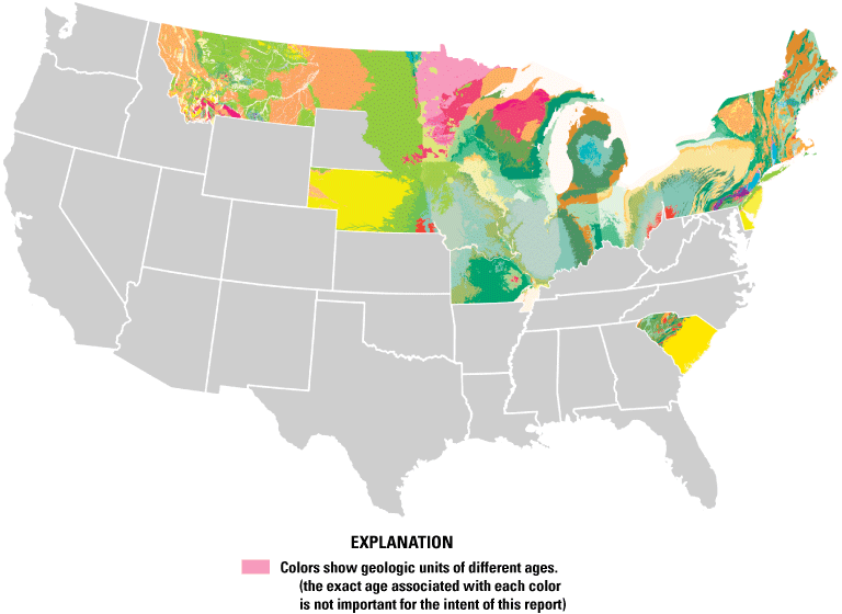
A map of the conterminous United States showing selections with different colors based on the geologic age of units. The colored areas were selected using the following query: SELECT mup.mapsourceid, mup.source_descriptionofmapunitsid, mup.source_mapunit, mup.mapunitpolys_id, mup.shape, CONCAT('rgba(',cs.rgba,')') AS rgba, ms.resolutionid, ms.geolayerid from source.mapunitpolys AS mup INNER JOIN assignments.age AS aa ON aa.source_descriptionofmapunitsid = mup.source_descriptionofmapunitsid INNER JOIN vocabularies.agedict AS cs ON cs.agedict_id = aa.agedictid_min INNER JOIN source.mapsources AS ms ON mup.mapsourceid = ms.mapsources_id WHERE ms.geolayerid = '3' AND ms.resolutionid = '2'
Selecting Polygons Whose Geomaterial Is or Derives from Intrusive Rock
All standard vocabularies have taxonomies represented by a hierarchy key. Searching based on this hierarchy key allows us to find anything that references a term directly or any of its descendants. The first part of the query in figure 1.6 populates the polygons with the attributes needed based on joins, including pulling in a standardized color from the geomaterial dict. The “where” clause in this query is populated by another query, which allows us to identify the hierarchy key used for searching the taxonomy based on the name of a geomaterial of interest, “Igneous rock.”
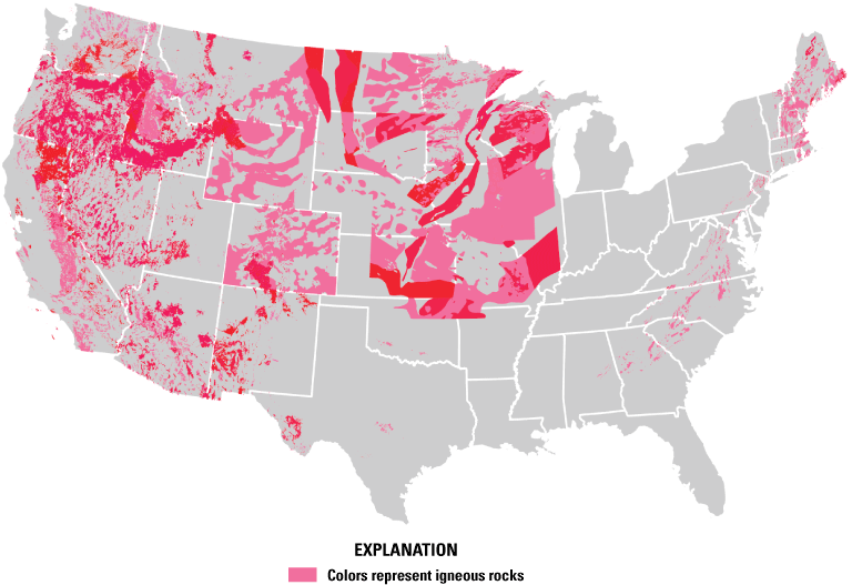
A map of the conterminous United States covered with a number of colored polygons representing igneous rocks. Igneous rocks were selected using the following query: SELECT mup.source_mapunit, shape, mapunitpolys_id, sdmu.geomaterial, gm.hierarchykey AS gm_hierarchy, CONCAT('rgba(',gm.rgba,')') as gm_rgba FROM source.mapunitpolys AS mup INNER JOIN source.source_descriptionofmapunits AS sdmu ON (mup.source_mapunit = sdmu.source_mapunit) INNER JOIN vocabularies.geomaterialdict AS gm ON (sdmu.geomaterial = gm.geomaterial) WHERE gm.hierarchykey LIKE CONCAT((SELECT hierarchykey FROM vocabularies.geomaterialdict WHERE geomaterial = 'Igneous rock'),'%')
Identifying Rocks of a Particular Age
The example in figure 1.7 mirrors the geomaterial and pre-Quaternary map colored by age example (fig. 1.5), now looking for all “Cretaceous” units. An added complication is that, although “geomaterial” is stored natively as a required GeMS component, the standard ages assigned by the synthesis database are related through the assignments.age table.
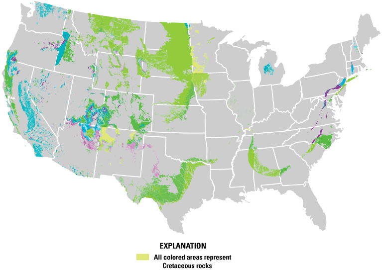
A map of the conterminous United States covered with a number of colored polygons representing Cretaceous rocks. Cretaceous units were selected using the following query: SELECT mup.source_mapunit, shape, mapunitpolys_id, sdmu.geomaterial, cs.hierarchykey AS cs_hierarchy,cs.age AS min_age, CONCAT('rgba(',cs.rgba,')') as cs_rgba FROM source.mapunitpolys AS mup INNER JOIN source.source_descriptionofmapunits AS sdmu ON (mup.source_mapunit = sdmu.source_mapunit) INNER JOIN assignments.age AS aa ON (aa.source_mapunit = sdmu.source_mapunit) INNER JOIN vocabularies.agedict AS cs ON (aa.agedictid_min = cs.agedict_id) WHERE cs.hierarchykey LIKE CONCAT((SELECT hierarchykey FROM vocabularies.agedict WHERE age = 'Mesozoic'),'%')
Age Text Replacement
Table 1.1 defines the text replacements used to facilitate mapping content in the source_descriptionofmapunits age field to standard minimum and maximum timescale terms in the agedict table. Text matches to the “from” column (after casting to lowercase) are replaced with the entries in the “to” column. These are then tokenized and searched for matches as described in the main text.
Table 1.1.
The replacements used for content in the source_descriptionofmapunits age field used to aid fuzzy matching to values from the timescale described in the agedict table.[Chronostratigraphic ages are from the International Chronostratigraphic Chart (Cohen and others, 2024)]
References Cited
Cohen, K.M., Harper, D.A.T., and Gibbard, P.L., 2024, ICS International Chronostratigraphic Chart, version 2024/12: International Commission on Stratigraphy, accessed February 13, 2025, at https://stratigraphy.org/chart#latest-version.
U.S. Geological Survey [USGS], 2006, FGDC digital cartographic standard for geologic map symbolization (PostScript implementation): U.S. Geological Survey Techniques and Methods 11–A2, accessed September 15, 2023, at https://doi.org/10.3133/tm11A2.
Datums
Horizontal coordinate information is referenced to North American Datum [NAD] 1983 Contiguous USA Albers, EPSG:5070. However, the coordinate system of the database described herein may be updated or change in the future; this does not affect the processes described in this report.
Abbreviations
2D
two-dimensional
3D
three-dimensional
CGI
Commission for Geoscience Information
DMU
description of map units
ETL
extract, transform, and load
FGDC
Federal Geographic Data Committee
GeMS
Geologic Map Schema
JSON
JavaScript Object Notation
NCGMP
National Cooperative Geologic Mapping Program
SGMC
State Geologic Map Compilation
USGS
U.S. Geological Survey
Publishing support provided by the Science Publishing Network,
Denver Publishing Service Center
For more information concerning the research in this report, contact the
Center Director, USGS Geosciences and Environmental Change Science Center
Box 25046, Mail Stop 980
Denver, CO 80225
(303) 236-5344
Or visit the Geosciences and Environmental Change Science Center website at
https://www.usgs.gov/centers/geosciences-and-environmental-change-science-center
Disclaimers
Any use of trade, firm, or product names is for descriptive purposes only and does not imply endorsement by the U.S. Government.
Although this information product, for the most part, is in the public domain, it also may contain copyrighted materials as noted in the text. Permission to reproduce copyrighted items must be secured from the copyright owner.
Suggested Citation
Johnstone, S.A., Colgan, J.P., and Roe, W.P., 2025, A synthesis engine for constructing geologic maps of the United States: U.S. Geological Survey Data Report 1210, 36 p., https://doi.org/10.3133/dr1210.
ISSN: 2771-9448 (online)
Study Area
| Publication type | Report |
|---|---|
| Publication Subtype | USGS Numbered Series |
| Title | A synthesis engine for constructing geologic maps of the United States |
| Series title | Data Report |
| Series number | 1210 |
| DOI | 10.3133/dr1210 |
| Publication Date | August 27, 2025 |
| Year Published | 2025 |
| Language | English |
| Publisher | U.S. Geological Survey |
| Publisher location | Reston VA |
| Contributing office(s) | Geosciences and Environmental Change Science Center |
| Description | Report: vi, 36 p.; Table; 4 Data Releases |
| Country | United States |
| Other Geospatial | conterminous United States |
| Online Only (Y/N) | Y |