

Range-wide Population Trend Analysis for Greater Sage-Grouse (Centrocercus urophasianus)—Updated 1960–2024
Links
- Document: Report (14 MB pdf) , HTML , XML
- Data Release: USGS data release - Trends and a targeted annual warning system for greater sage-grouse in the western United States (ver. 4.0, November 2025)
- Download citation as: RIS | Dublin Core
Acknowledgments
We performed this update and original modeling analysis in close consultation with the Bureau of Land Management, Western State wildlife agencies, and the U.S. Fish and Wildlife Service. We extend gratitude for the cooperation of personnel from Western State wildlife agencies, who provided feedback at several stages on uses of lek data, modeling methods, and constructive reviews at several stages of production. Specifically, we value the contributions from Tom Remington and San Stiver; Shawn Espinosa and Justin Small (Nevada Department of Wildlife); Kathy Griffin (Colorado Parks and Wildlife); Katherine Miller (California Department of Fish and Wildlife); Ann Moser, Michelle Kemner, and Jennifer Struthers (Idaho Department of Fish and Game); Avery Cook ([formerly] Utah Division of Wildlife Resources); Ashley Green and Heather Talley (Utah Division of Wildlife Resources); Jesse Kolar (North Dakota Game and Fish Department); Travis Runia and Alex Solem (South Dakota Department of Game, Fish, and Parks); Mike Schroeder and Michael Atamian (Washington Department of Fish and Wildlife); Catherine Wightman ([formerly] Montana Department of Fish, Wildlife and Parks); Heather Harris (Montana Department of Fish, Wildlife and Parks); Lee Foster, Skyler Vold, and Mikal Cline (Oregon Department of Fish and Wildlife). We also thank the Wyoming Game and Fish Department for providing data for this analysis. We thank Katie Andrle (Nevada Department of Wildlife), Kelly McGowan (Nevada Sagebrush Ecosystem Technical Team), Matt Magaletti, Arlene Kosic, and Megan McLachlan (Bureau of Land Management); John Tull ([formerly] U.S. Fish and Wildlife Service); Steve Abele (U.S. Fish and Wildlife Service); Scott Gardner and Brian Ehler (California Department of Fish and Wildlife), for their input throughout the initial components of this study. We thank Elliott Matchett and Jonathan Rose of the U.S. Geological Survey for helpful comments in reviewing this data report in its entirety. This project could not have been completed without the financial support of the Bureau of Land Management and the U.S. Geological Survey. Funds for the pilot efforts were also provided by the Bureau of Land Management-Nevada and the Nevada Department of Wildlife. Parts of this report were written following a previously developed template (Coates and others, 2022a) to maintain consistent presentation of results.
Abstract
Greater sage-grouse (Centrocercus urophasianus; hereafter sage-grouse) are at the center of State and national land-use policies largely because of their unique life-history traits as an ecological indicator for the health of sagebrush ecosystems. This updated population trend analysis provides State and Federal land and wildlife managers with the best available science to help guide management and conservation plans aimed at benefiting sage-grouse populations and the ecosystems they inhabit. This analysis relied on previously published population trend modeling methodology from Coates and others (2021, 2022a) and incorporates population lek count data for 1960–2024. Included in this report are methodological updates to lek count data aggregation, state-space model forecasting, and targeted annual warning system signals, which are detailed under individual Modification sections. State-space models estimated a 2.9-percent average annual decline in sage-grouse populations between 1966 and 2021 (Period 1, six population oscillations) across their geographical range. The average annual decline among climate clusters for the same number of oscillations ranged between 2.2 and 3.4 percent. Cumulative declines were 41.2, 64.1, and 78.8 percent range-wide in Period 5 (19 years), Period 3 (35 years), and Period 1 (55 years), respectively.
Introduction
As of the turn of the 21st century, sage-grouse occupied roughly half of their former historical range (Schroeder and others, 2004; Miller and others, 2011), and populations have subsequently experienced marked declines in many parts of their current range (Garton and others, 2011; Western Association of Fish and Wildlife Agencies, 2015). A 2021 study led by the U.S. Geological Survey (USGS), in cooperation with the Bureau of Land Management (BLM) and Western State wildlife agencies, revealed an approximately 3.1-percent annual average population decline range-wide (Coates and others, 2021). However, variation in trends was described across different spatial and temporal scales.
Decades of past research have attributed sage-grouse population declines to loss and fragmentation of sagebrush communities as well as to a suite of environmental stressors (Remington and others, 2021). Since 1999, sage-grouse have been petitioned for legal protection under the Endangered Species Act (ESA) on nine occasions, and actions to conserve and restore sage-grouse habitats are now central to guiding land-management actions and policies across most of the western United States. Specifically, the resource needs of sage-grouse have been used to help guide management and restoration actions aimed at improving conditions in sagebrush ecosystems, with resultant practices thought to benefit other sagebrush-dependent species (Rowland and others, 2006; Hanser and Knick, 2011; Dinkins and others, 2021). Sage-grouse are considered an indicator for the function of sagebrush ecosystems (Prochazka and others, 2023) and an umbrella for the protection of other sagebrush-obligate or sagebrush-dependent species because of their near-complete reliance on sagebrush ecosystems (Rich and Altman, 2001; Rich and others, 2005; Rowland and others, 2006; Hanser and Knick, 2011). Importantly, several Federal resource management plan amendments accompanying the U.S. Fish and Wildlife Service (USFWS) “not warranted” 2015 ESA listing determination called for greater integration of sage-grouse management into their land-use planning, specifically identifying how to implement adaptive management. An unprecedented level of conservation effort and planning among Federal (Bureau of Land Management, 2015; U.S. Department of Agriculture Forest Service, 2015a, b), State, and private stakeholders was identified as the primary driver for the USFWS decision in the most recent (2015) status assessment (U.S. Fish and Wildlife Service, 2015).
The purpose of this report is to provide updated results on sage-grouse population analyses (trends in abundance, extirpation probabilities, targeted annual warning system [TAWS]) across their geographical range in the western United States. This report reflects previous modeling methodologies (Coates and others, 2021, 2022a), describes updates to those methodologies, and includes additional data to inform population analyses through 2024. A detailed description of data collection and compilation, population clustering methods to identify spatial extents, and modeling methodologies was provided in the first three objectives described in Coates and others (2021). Additional methodologies developed since Coates and others (2021) are described in Coates and others (2022a) and in this report. The USGS, in cooperation with the BLM, are providing this scientific information to fulfill a prominent information gap, thus informing the adaptive management of sage-grouse populations, as well as monitoring and conservation management strategies. The ongoing collaborative effort between the USGS Western Ecological Research Center (WERC), Fort Collins Science Center (FORT), Colorado State University (CSU), BLM, USFWS, and Western State wildlife agencies aims to update and improve the hierarchical monitoring framework for sage-grouse within sagebrush ecosystems. These updates include a technical transfer of improved documentation (for example, frequently asked questions, numerous information sheets, and web pages), training, and regular meetings, all of which have added great value to improving the science that informs management.
Study Area
Our study extent consisted of the geographic range of sage-grouse in the United States and was described previously in Coates and others (2021). Briefly, this area represents the sagebrush biome occurring across western North America and extending east from the Sierra Nevada and Cascade Mountain ranges to the western regions of the Great Plains of the United States. The vegetation communities vary in precipitation, temperature, soils, topographic position, and elevation (Miller and others, 2011). The most abundant shrub species include sagebrush (Artemisia spp.), along with less abundant non-sagebrush species, such as rabbitbrush (Chrysothamnus spp.), horsebrush (Tetradymia spp.), greasewood (Sarcobatus spp.), common snowberry (Symphoricarpos spp.), serviceberry (Amelanchier spp.), fourwing saltbush (Atriplex spp.), and bitterbrush (Purshia spp.). The primary native herbaceous species include wheatgrass (Agropyron spp.), fescue (Festuca spp.), bluegrass (Poa spp.), needlegrass (Stipa spp.), and squirreltail (Elymus spp.), whereas less abundant forb species include phlox (Phlox spp.), milk-vetch (Astragalus spp.), and fleabane (Erigeron spp.). Non-native annual grasses, such as cheatgrass (Bromus tectorum), are prevalent across the range and can represent the dominant component of plant communities in many areas.
Data Compilation and Inputs
We developed a single unified database from all digitized field observations of sage-grouse lek counts completed since 1941 and compiled by all State wildlife agencies that monitored sage-grouse populations during that time. We worked with each State agency to ensure the fullest understanding of the data to maximize the number of appropriate records kept in the database. We addressed spatial errors, and we reviewed all data products with Western State wildlife agency biologists. Data compilation rules and the detailed methodology used in these analyses were published in Coates and others (2021, 2022a) and O’Donnell and others (2021). The additional years of data (through 2024) used to update these analyses followed the exact quality assessment and quality control (QA/QC) measures described in the previous publications and included additional updates described in this report. Using all the rules for selecting data appropriate for population modeling, we retained 112,699 observations (88,596; TAWS) across 5,514 leks (4,914; TAWS). The fewer number of observations and leks used in the TAWS stems from the more narrow and contemporary focus of that analysis, which aims to identify sustained, aberrant population declines that can be addressed now or in the near future. The sage-grouse lek data used in this update either are not publicly available or have limited availability owing to unique restrictions held by each State (data are managed by 11 Western States and are not public due to the sensitivity of the species and State regulations, policies, or laws). Individual Western State wildlife agencies (see the “Acknowledgments” section) can be contacted for additional information.
Changes in population abundance are affected by environmental factors that operate on multiple spatial and temporal scales, which follow ecological rather than geopolitical boundaries. Hence, we examined population trends across biologically relevant and hierarchically nested units to improve the detection of factors driving change across multiple spatial scales. We grouped sage-grouse lek sites into hierarchically nested clusters or populations using least-cost minimum spanning trees, a clustering algorithm, and a suite of relevant biotic and abiotic spatial products described in O’Donnell and others (2022). Briefly, we selected two cluster levels to represent a fine (neighborhood cluster [NC]) and a broad spatial scale (climate cluster [CC]). Model output included estimated apparent abundance (; hereafter abundance) and intrinsic rates of population change () at the lek, NC, and CC levels. These parameters were used to calculate abundance indices and average annual rates of change in abundance ().
Range-Wide Sage-Grouse Population Model
Detailed formulation of the sage-grouse population model was described in Coates and others (2021). Coates and others (2022a) describe analytical updates that (1) identify population nadirs (two lowest points within a single complete population oscillation denoting the start and end of a single period) at spatial scales of the lek (breeding ground) and neighborhood cluster (group of leks) and (2) truncate prior probability distributions on rate of change in abundance parameters to more realistic boundaries for leks with missing data. Briefly, we used a state-space model (SSM) that relied on Markov chain Monte Carlo sampling, using Bayesian inference, to derive posterior probability distributions (PD) of and using lek count data across the sage-grouse geographical range. This approach allowed inferences for each lek, as well as higher-order, nested spatial extents, such as NC and CC, in each year of the time series. Advantages and assumptions inherent to the SSM approach were described in Coates and others (2021, 2022a).
Modification 1—Inclusion of Maximum Counts Outside Peak Attendance Periods
We modified the original methodology (Coates and others, 2021, page 7) for identifying field observations within the sage-grouse lek database that maximized detection probabilities of lek attendance and minimized errors in counting males. Specifically, we amended Rule 1 (select observations recorded from March 1 to May 31) and Rule 2 (select observations recorded within 30 minutes before and 90 minutes after local sunrise) by maintaining counts recorded outside peak attendance dates and sunrise timeframes, but only when those counts exceeded counts recorded within peak timeframes (assessed per lek per year). If a lek had a single count recorded for a given year, and that count was outside peak attendance timeframes, it was removed from the dataset. These modifications to Rule 1 and Rule 2 ensured that the maximum number of males observed for a given lek and year informed model estimates, while avoiding the use of counts that were biased low due to collection outside peak timeframes. Rules 3–6 remained unchanged from the original methodology (Coates and others, 2021).
Modification 2—Forecasting Abundance Outside the Model
Fitting SSMs to count data collected from populations that experience annual cycles or oscillations in abundance can be problematic when predicting future population sizes. The model’s weakness stems from the Markovian process, which propagates using expected values of population change () for the entire time series and the previous year’s estimated abundance, irrespective of location in the population cycle. The updated method described here obviates this issue by propagating future values from the most recent nadir using values of population change from every historically complete population oscillation. We modified the original methodology (Coates and others, 2021) for estimating future population sizes (forecasting abundance) by deriving values outside the SSM using posterior distributions (PDs) of (associated with the most recent nadir) and (spanning Nadirs 1–7; table 1). This method produces identical estimates to a model fit to data restricted to the same timeframe but is more desirable because it can be applied regardless of where populations are at in their cycle. Most notably, the updated method will provide more realistic expectations of future extirpation probabilities when the final year of a dataset does not coincide with a nadir in the population cycle.
Table 1.
Identified years of population abundance nadirs (lowest points within cycles) used to define temporal scales (Period 1–Period 6) of population trend estimates across different climate clusters (A–F) and range-wide for greater sage-grouse (Centrocercus urophasianus) in the western United States.[A, Bi-State area; B, Washington area; C, Jackson Hole, Wyoming area; CC, climate cluster; D, eastern area; E, Great Basin area; F, western Wyoming area]
Modification 3—Chronic Warnings for a Targeted Annual Warning System
The TAWS framework was originally developed with a focus on rates of population change and if a population at a management scale (lek, neighborhood cluster) had declined and decoupled from a larger, spatially nested reference scale (climate cluster). That focus considered the relationship within a relatively narrow moving window (as many as 4 years in length) and disregarded the potential for chronic effects. Based on feedback from State and Federal agency personnel, we developed a novel signal (warningN) that considered chronic effects within the context of aberrant losses in abundance. These chronic warnings (warningN) activate concurrently with traditional warnings but remain in place until abundance rebounds to a similar relative level of abundance shown at the larger scale (climate cluster). Specifically, we recorded the median of the affected population (lek, neighborhood cluster) for the year that preceded the first signal leading to a traditional warning. That value represented the last unperturbed population size. We then developed a time series of expected spanning every subsequent year, up to the present time, using annual estimates of at the climate cluster scale. Deriving expectations of abundance at the management scale (lek, neighborhood scale), using rates of population change () at the climate scale, allowed for a dynamic evaluation that considered broader trends in abundance. The chronic warning (warningN) was only deactivated once the median at the affected management scale matched or surpassed the expected .
Modification 4—Additional Year of Data
The previously published analyses included data from 1960 to 2023 (Prochazka and others, 2024). In this report, we updated the model to include lek count data collected in 2024 across the sage-grouse geographic range. Lek count data collected in 2024, within the State of Wyoming, were restricted to Federally managed public lands (n=974 leks). The removal of 2024 lek count data collected from private and State-managed public lands in Wyoming resulted in 813 fewer lek counts compared to the preceding 10-year average (n=1,787; 2014–23). Because SSMs estimate changes in population size using a Markov process (state at time t+1 depends on state at time t) and because an additional year of data has been included, trends and warnings reported herein may reveal slight shifts from the previous report (Prochazka and others, 2024). This version of the analysis supersedes previous reports and represents trends across different spatial extents (leks, NCs, and CCs) and temporal periods (for example, 2024 back-in-time to each population nadir) across the geographic range of sage-grouse.
Range-Wide Population Trends
Our model fit the observed data well (Bayesian p-value=0.50). Median from the SSM revealed seven distinct range-wide population nadirs across the 65 years of data, which were 1966, 1975, 1986, 1996, 2002, 2013, and 2021. The range-wide, across-years, mean male count was 17.5 per lek (95-percent confidence interval [CI]=17.4–17.6). The number of years per complete population oscillation (nadir-to-nadir) was relatively consistent across periods (average=9.1; 95-percent CI=4.9–15.0; table 1). Model estimates revealed evidence of range-wide decline, on average, from every historic abundance nadir to 2021 (fig. 1; table 2); for example, the average annual for Period 5 (19 years, two oscillations), Period 3 (35 years, four oscillations), and Period 1 (55 years, six oscillations) was 0.971 (median; 95-percent credible interval [CRI]=0.969–0.973), 0.970 (median; 95-percent CRI=0.968–0.972), and 0.972 (median; 95-percent CRI=0.970–0.974), respectively. These trends imply declines of 41.2, 64.1, and 78.8 percent, relative to population sizes observed 19, 35, and 55 years earlier, respectively. In an earlier version of the model (Coates and others, 2021), we specified the final nadir for all populations using the final year of the dataset (2019), which was the lowest point of for most populations at that time. A more recent report provided an update of the original analysis and included years 2020–23 (Prochazka and others, 2024). In that report, researchers concluded that not all populations had reached a nadir in 2019. The additional year of count data (2024) provided in this report supports previous conclusions of 2021 being the most recent nadir for populations at the range-wide scale. Trends estimated at CC (fig. 2) and NC (fig. 3) scales are generally consistent with the previous report (Prochazka and others, 2024). We estimated median to be less than 1.0 for 89.5, 92.3, and 97.7 percent of NCs in Period 5, Period 3, and Period 1, respectively, throughout the sage-grouse range.

Abundance index (calculated as divided by 65-year mean of ) of greater sage-grouse (Centrocercus urophasianus) across their range from lek observations used to model population trends from 1960 to 2024. Median estimates (solid-colored lines) and 95-percent credible limits (dashed colored lines) of abundance trend in Period 5 (two oscillations), Period 3 (four oscillations), and Period 1 (six oscillations). Black trend line represents median estimates. Colored areas represent 95-percent credible limits of trend estimates. Gray shaded areas represent 95-percent credible limits on abundance index. Trend estimates extend beyond Nadir 7 to serve as a reference to abundance indices in subsequent years.
Table 2.
Greater sage-grouse (Centrocercus urophasianus) median annual rate of population change () and 95-percent credible interval across six temporal scales that correspond to Period 1 (six oscillations), Period 2 (five oscillations), Period 3 (four oscillations), Period 4 (three oscillations), Period 5 (two oscillations), and Period 6 (one oscillation) for each climate cluster in the western United States (see table 1).[A, Bi-State area; B, Washington area; C, Jackson Hole, Wyoming area; CC, climate cluster; D, eastern area; E, Great Basin area; F, western Wyoming area]
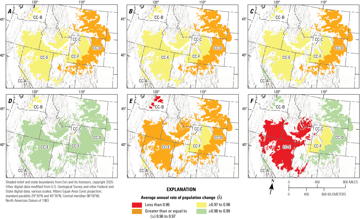
Range-wide spatial estimates of average annual rate of change () in abundance of greater sage-grouse (Centrocercus urophasianus) across six temporal scales based on periods of oscillation: A, Period 1 (six oscillations); B, Period 2 (five oscillations); C, Period 3 (four oscillations); D, Period 4 (three oscillations); E, Period 5 (two oscillations); and F, Period 6 (one oscillation) for each climate cluster (CCs; A–F).

Range-wide spatial estimates of average annual rate of change () in abundance of greater sage-grouse (Centrocercus urophasianus) across six temporal scales based on periods of oscillation: A, Period 1 (six oscillations); B, Period 2 (five oscillations); C, Period 3 (four oscillations); D, Period 4 (three oscillations); E, Period 5 (two oscillations); and F, Period 6 (one oscillation) for each neighborhood cluster.
Climate Cluster Population Trends
Climate cluster A (CC-A; Bi-State area) consisted of 11 NCs that encompassed 726,907 hectares (ha). Two NCs lacked sufficient lek count data to estimate trends. Climate cluster A consisted of 96 leks, representing approximately 1 percent of the range-wide database. After QA/QC, 61 leks met criteria for use in the SSM (table 2), totaling 1,788 field observations. Mean male count was 20.2 (95-percent confidence interval=18.9–21.5). For CC-A, we estimated six population abundance nadirs that dated back to 1960 and included nadirs of 1969, 1977, 1983, 1995, 2002, 2008, and 2019 (table 1). We estimated for Period 5 (2002–19, two oscillations, 17 years), Period 3 (1983–2019, four oscillations, 36 years), and Period 1 (1969–2019, six oscillations, 50 years) as 0.975 (95-percent CRI=0.962–0.984), 0.987 (95-percent CRI=0.973–0.998), and 0.978 (95-percent CRI=0.967–0.987), respectively (table 2). In the past 17, 36, and 50 years, sage-grouse populations have experienced declines in abundance equal to 33.8, 36.6, and 67.1 percent, respectively (fig. 4A). We estimated median to be less than 1.0 for all NCs in Period 5, Period 3, and Period 1, respectively.

Abundance index (calculated as divided by 65-year mean of ) of greater sage-grouse (Centrocercus urophasianus) in climate clusters (CCs) A, (CC-A; Bi-State area); B, (CC-B; Washington area); C, (CC-C; Jackson Hole, Wyoming area); D, (CC-D; Eastern area); E, (CC-E; Great Basin area); and F, (CC-F; western Wyoming area). Lek observations were used to model population trends from 1960 to 2024. Median estimates (solid-colored lines) and 95-percent credible limits (dashed colored lines) of abundance trends across temporal scales based on periods of oscillation: Period 5 (two oscillations), Period 3 (four oscillations), and Period 1 (six oscillations), right to left. Colored areas represent 95-percent credible limits of trend estimates. Orange lines and gray shaded areas represent median and 95-percent credible limits on abundance index, respectively.
Climate cluster B (CC-B; Washington area) consisted of four NCs that encompassed 1,139,954 ha. One NC lacked sufficient lek count data to estimate trends. Climate cluster B consisted of 54 leks, representing approximately 0.6 percent of the lek database. After QA/QC, 43 leks met criteria for use in the state-space trend model (table 2), totaling 1,237 field observations. Mean male count was 14.2 (95-percent confidence interval=13.3–15.0). For CC-B, we estimated six population abundance nadirs that dated back to 1960 and included 1964, 1976, 1986, 1994, 2008, 2017, and 2023 (table 1). We estimated for Period 5 (2008–23, two oscillations, 15 years), Period 3 (1986–2023, four oscillations, 37 years), and Period 1 (1964–2023, six oscillations, 59 years) as 0.959 (95-percent CRI=0.947–0.971), 0.977 (95-percent CRI=0.967–0.984), and 0.972 (95-percent CRI=0.964–0.981), respectively (table 2). In the past 15, 37, and 59 years, sage-grouse populations have experienced declines in abundance equal to 44.3, 56.8, and 80.2 percent, respectively (fig. 4B). We estimated median to be less than 1.0 for all NCs in Period 5, Period 3, and Period 1, respectively.
Climate cluster C (CC-C; Jackson Hole, Wyoming area) consisted of two NCs that encompassed 66,733 ha. Climate cluster C consisted of 17 leks, representing approximately 0.2 percent of the lek database. After QA/QC, 14 leks met criteria for use in the SSM (table 2), totaling 352 field observations. Mean male count was 13.5 (95-percent confidence interval=11.9–15.2). For CC-C, we estimated population abundance nadirs in 1963, 1969, 1984, 1999, 2003, 2011, and 2019 (table 1). We estimated for Period 5 (2003–19, two oscillations, 16 years), Period 3 (1984–2019, four oscillations, 35 years), and Period 1 (1963–2019, six oscillations, 56 years) as 0.965 (95-percent CRI=0.946–0.982), 0.970 (95-percent CRI=0.943–0.992), and 0.966 (95-percent CRI=0.949–0.986), respectively (table 2). In the past 16, 35, and 56 years, sage-grouse populations have experienced declines in abundance equal to 41.8, 64.6, and 85.2 percent, respectively (fig. 4C). We estimated median to be less than 1.0 for all NCs across this temporal scale.
Climate cluster D (CC-D; Eastern area) consisted of 169 NCs that encompassed 25,920,530 ha. There were 23 NCs that lacked sufficient lek count data to estimate trends. Climate cluster D consisted of 3,096 leks, representing approximately 35.2 percent of the lek database. After QA/QC, 1,926 leks met criteria for use in the SSM (table 2) and totaled 38,565 field observations. Mean male count was 16.3 (95-percent confidence interval=16.0–16.5). For CC-D, we estimated six population abundance nadirs that dated back to 1960 and included 1966, 1981, 1986, 1997, 2004, 2013, and 2019 (table 1). We estimated for Period 5 (2004–19, two oscillations, 15 years), Period 3 (1986–2019, four oscillations, 33 years), and Period 1 (1966–2019, six oscillations, 53 years) as 0.960 (95-percent CRI=0.956–0.963), 0.968 (95-percent CRI=0.963–0.972), and 0.967 (95-percent CRI=0.963–0.972), respectively (table 2). In the past 15, 33, and 53 years, sage-grouse populations have experienced declines in abundance equal to 43.6, 64.4, and 82.9 percent, respectively (fig. 4D). We estimated median to be less than 1.0 for 91.4, 95.0, and 99.3 percent of NCs in Period 5, Period 3, and Period 1, respectively.
Climate cluster E (CC-E; Great Basin area) consisted of 241 NCs that encompassed 34,627,182 ha. There were 17 NCs that lacked sufficient lek count data to estimate trends. Climate cluster E consisted of 4,252 leks, representing approximately 48.3 percent of the lek database. After QA/QC, 2,452 leks met criteria for use in the SSM (table 2) and totaled 47,392 field observations. Mean male count was 16.0 (95-percent confidence interval=15.8–16.2). For CC-E, we estimated six population abundance nadirs that dated back to 1960 and included 1967, 1975, 1985, 1996, 2002, 2013, and 2021 (table 1). We estimated for Period 5 (2002–21, two oscillations, 19 years), Period 3 (1985–2021, four oscillations, 36 years), and Period 1 (1967–2021, six oscillations, 54 years) as 0.967 (95-percent CRI=0.964–0.970), 0.974 (95-percent CRI=0.970–0.977), and 0.972 (95-percent CRI=0.970–0.974), respectively (table 2). In the past 19, 36, and 54 years, sage-grouse populations have experienced declines in abundance equal to 45.0, 60.2, and 77.6 percent, respectively (fig. 4E). We estimated median to be less than 1.0 for 86.9, 89.6, and 97.3 percent of NCs in Period 5, Period 3, and Period 1, respectively.
Climate cluster F (CC-F; western Wyoming area) consisted of 56 NCs that encompassed 8,899,755 ha. Three NCs lacked sufficient lek count data to estimate trends. Climate cluster F consisted of 1,291 leks, representing approximately 14.7 percent of the lek database. After QA/QC, 1,018 leks met criteria for inclusion in the SSM (table 2) and totaled 23,365 field observations. Mean male count was 22.6 (95-percent confidence interval=22.2–23.0). For CC-F, we estimated six population abundance nadirs that dated back to 1960 and included 1966, 1975, 1987, 1996, 2002, 2013, and 2021 (table 1). We estimated for Period 5 (2002–21, two oscillations, 19 years), Period 3 (1987–2021, four oscillations, 34 years), and Period 1 (1966–2021, six oscillations, 55 years) as 0.975 (95-percent CRI=0.971–0.980), 0.970 (95-percent CRI=0.965–0.974), and 0.975 (95-percent CRI=0.971–0.979), respectively (table 2). In the past 19, 35, and 55 years, sage-grouse populations have experienced declines in abundance equal to 36.5, 64.7, and 74.1 percent, respectively (fig. 4F). We estimated median to be less than 1.0 for 92.5, 94.3, and 94.3 percent of NCs in Period 5, Period 3, and Period 1, respectively.
Neighborhood cluster trends for different temporal scales that are not listed in this report can be viewed in Coates and others (2022b). Coates and others (2022b) is the data release that accompanies this updated (1960–2024) report.
Probability of Future Extirpation
Expanding on the population analyses, we projected for each lek and NC across three temporal scales that reflected two, four, and six future oscillations using the same model and dataset. We used the mean duration of one complete oscillation (9.1 years) based on estimated from SSM results. We then calculated the proportion of the posterior probability distribution of that was less than two males (the minimum number to represent a lek) for the last prediction year of each temporal scale. Although this value is not true extirpation (zero birds), we refer to it as extirpation to align with State definitions of lek inactivity. Extirpation of leks within NCs was thought to reflect a loss of a metapopulation resulting from reduced demographic rates.
The mean extirpation probability calculated across all leks was 0.50 (standard deviation [SD]=0.32), 0.58 (SD=0.28), and 0.63 (SD=0.27) for two (fig. 5A), four (fig. 5B), and six (fig. 5C) future oscillations, respectively. However, distributions of predicted extirpation rates for leks appeared bimodal with peak probabilities near 0.08 and 0.93 (two oscillations, fig. 5A), 0.26 and 0.94 (four oscillations, fig. 5B), and 0.43 and 0.98 (six oscillations, fig. 5C). Approximately 51, 58, and 65 percent of leks possessed an extirpation probability greater than 0.5 for two, four, and six oscillations, respectively. The spatial distribution of lek extirpation probabilities demonstrated higher concentrations of higher probabilities at the edges of the species range (figs. 6A–C). The mean extirpation probability calculated across all NCs was 0.16 (SD=0.27), 0.24 (SD=0.30), and 0.32 (SD=0.31) for two (fig. 5D), four (fig. 5E), and six (fig. 5F) future oscillations, respectively. Approximately 13, 19, and 29 percent of NCs possessed an extirpation probability greater than 0.5 for two, four, and six oscillations, respectively. The highest probabilities of NC scale extirpation often occurred at the periphery of the species range (figs. 6D–F). Conversely, interior NCs consisted primarily of low extirpation probabilities ranging from 0 to 0.25.
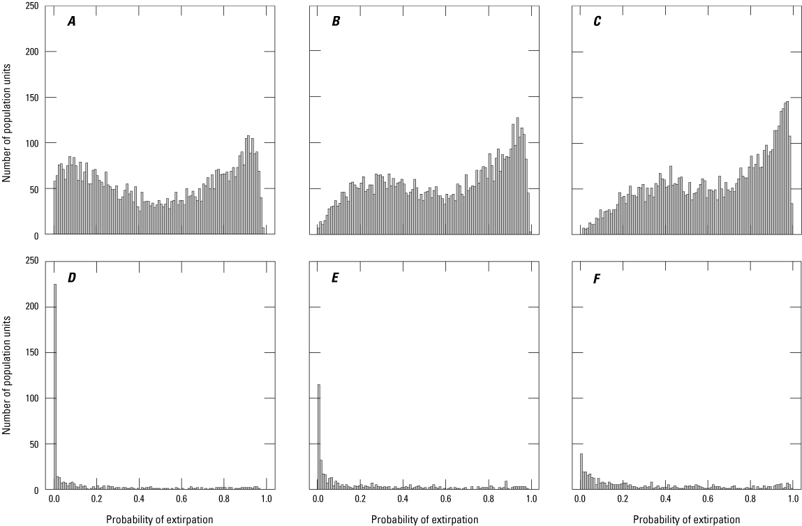
Range-wide extirpation probabilities calculated for greater sage-grouse (Centrocercus urophasianus) populations in the western United States using two spatial (lek, neighborhood cluster) and three temporal (two future oscillations [18.2 years], four future oscillations [36.4 years], six future oscillations [54.6]) scales. Lek extirpation probabilities have a bimodal distribution at A, two; B, four; and C, six oscillations. Neighborhood cluster extirpation probabilities calculated over the same temporal scales (D, two; E, four; and F, six) peak at zero and have a strong positive skew. Extirpation probabilities were calculated as the proportion of posterior samples with less than two sage-grouse.
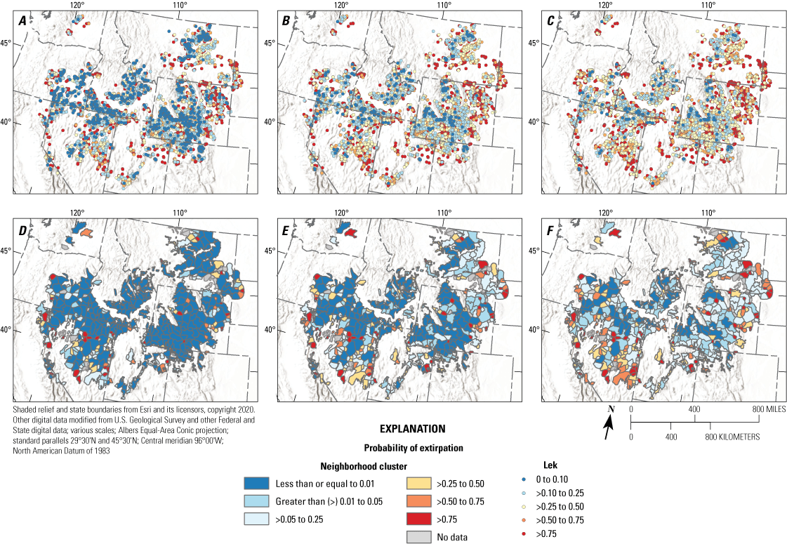
Spatial and temporal depictions of range-wide extirpation probabilities for greater sage-grouse (Centrocercus urophasianus) populations within the western United States using two spatial (lek, neighborhood cluster) and three temporal (two future oscillations [18.2 years], four future oscillations [36.4 years], six future oscillations [54.6]) scales. Lek extirpation probabilities calculated from A, two; B, four; and C, six oscillations were based on an average period length of 9.1 years. Neighborhood cluster extirpation probabilities (D, two; E, four; and F, six) were calculated over the same temporal scales. Extirpation probabilities were calculated as the proportion of posterior samples with less than two sage-grouse.
Neighborhood cluster extirpation probabilities for different temporal scales that are not listed in this report can be viewed in Coates and others (2022b). Coates and others (2022b) is the data release that accompanies this updated (1960–2024) report.
Watches and Warnings from a Targeted Annual Warning System
The TAWS is a hierarchical monitoring strategy that contrasts estimates of across nested spatial scales on an annual basis. Comparisons can act as a powerful analytical tool to help target when and where to adjust monitoring efforts, or inform where to carry out management actions. Methodology of TAWS was described in detail in Coates and others (2021) and Prochazka and others (2023). The TAWS produces signals referred to as watches and warnings, which signify progressively greater degrees of evidence for aberrant decline. Evidence of aberrant decline is assessed using independent sets of standardized thresholds that seek to stabilize the range-wide population (range-wide thresholds) versus individual climate clusters (climate cluster thresholds). The original published report (Coates and others, 2021) describing TAWS results presented each set of thresholds to provide managers with multiple strategic options. Here, we chose to report TAWS results using CC thresholds based on feedback of implementation from State and Federal agency personnel. The primary reason for the preferential use of CC thresholds is the superior performance in targeting peripheral and sparsely distributed populations. Like the trend analysis, thousands of historic lek surveys underwent QA/QC, as described in the results of Objective 1 for the TAWS analysis (Coates and others, 2021).
From 1990 to 2024, we estimated 72.5 and 57.8 percent of 4,914 sage-grouse leks experienced at least one watch or warning (table 3), respectively, across the species’ range. We calculated a mean annual percentage of leks that experienced a first watch or warning (no watches or warnings in any preceding year) to be 2.1 (105 leks) and 1.7 percent (84 leks), respectively. The mean annual percentage of leks that experienced a repeat watch or warning (at least one watch or warning occurred in a preceding year) was 5.9 (291 leks) and 6.1 percent (300 leks), respectively. Climate cluster A had the greatest percentage of watches at leks across the 35 years, where 92.6 percent of leks activated one or more times (table 3). Conversely, CC-E consisted of the greatest number of watches compared to other clusters (number of first watches=1,501; number of repeat watches=4,048; table 3). Climate cluster C had the lowest percentage of watches, at 64.3 percent (number of first and repeat watches=9 and 41, respectively; table 3). Climate cluster F had the greatest percentage (74.9) of warnings, whereas CC-E had the greatest number (first=1,151 and repeat=4,203). The second-highest percentage of watches (89.7) occurred in CC-F, whereas the second-highest percentage of warnings (72.2) occurred in CC-A.
Table 3.
Watches and warnings identified at greater sage-grouse (Centrocercus urophasianus) leks and neighborhood clusters (NC) across climate clusters (A–F) using state-space model estimates within a targeted annual warning system in the western United States from 1990 to 2024.[Number of watches and warnings that include repeat (r), only first time (f), and proportion (p) of populations (lek or NC) are reported. Abbreviations: A, Bi-State area; B, Washington area; C, Jackson Hole, Wyoming area; CC, climate cluster; D, eastern area; E, Great Basin area; F, western Wyoming area]
From 1990 to 2024, we estimated 60.6 and 46.7 percent of 426 NCs experienced at least one watch or warning (table 3), respectively, across the species’ range. An average of 1.8 (repeat=0.051) and 1.4 (repeat=0.047) percent of clusters activated per year, which was approximately 7.6 (repeat=21.5) and 5.9 (repeat=20.0) clusters annually. We reported that CC-A and CC-E had the greatest percentage (88.9, 79.1) of watches, whereas CC-E had the greatest number (first=174 and repeat=546) of watches across the 35-year timeframe. For warnings, CC-A had the greatest percentage (77.8; table 3), and CC-E had the greatest number (first=130 and repeat=476).
In 2024, we estimated 0.7 and 0.8 percent of leks experienced a first watch and warning, respectively, range-wide (table 4), which equated to 33 (repeat=123; fig. 7) first watches and 40 (repeat=407; fig. 7) first warnings. In 2024, the greatest percentage of first watches (1.6) and warnings (1.5) were within CC-D, which were 27 (repeat=66) first watches and 26 (repeat=175) first warnings (table 4). In 2024, we estimated 0.5 and 0.2 percent of neighborhoods experienced a first watch and warning, respectively, range-wide (table 4), which equated to 2 (repeat=8; fig. 8) first watches and 1 (repeat=28; fig. 8) first warning. Climate cluster D experienced the greatest percentage of NC watches (1.4) and warnings (0.7) in 2024. No other NC experienced a new watch or warning in 2024. Warnings and watches for each neighborhood cluster are available in Coates and others (2022b).
Table 4.
Watches and warnings identified at the lek and neighborhood cluster (NC) scales across different climate clusters (A–F) using state-space model estimates within a targeted annual warning system framework for greater sage-grouse (Centrocercus urophasianus) across their range in the western United States in 2024.[Number of watches and warnings that include repeat (r), only first time (f), and proportion (p) of populations (lek or NC) are reported. Abbreviations: A, Bi-State area; B, Washington area; C, Jackson Hole, Wyoming area; CC, climate cluster; D, eastern area; E, Great Basin area; F, western Wyoming area]
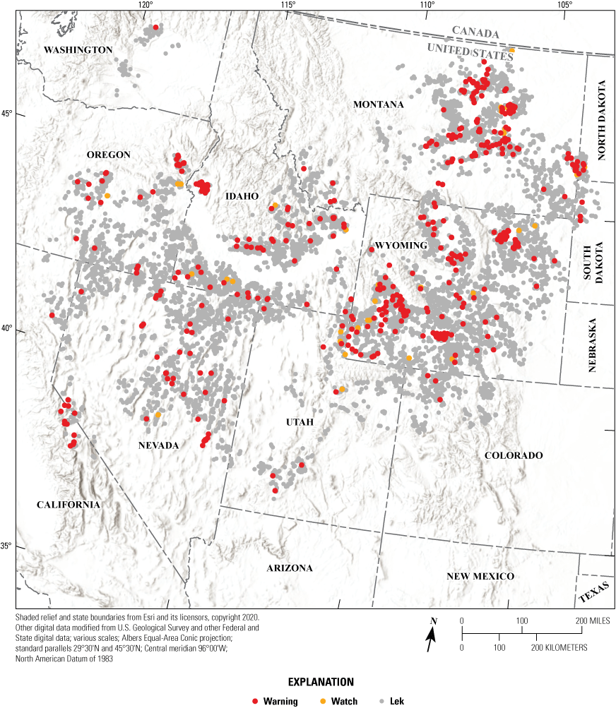
Spatial depiction of range-wide watches and warnings of greater sage-grouse (Centrocercus urophasianus) population declines at the lek scale in the western United States in 2024.

Spatial depiction of range-wide watches and warnings of greater sage-grouse (Centrocercus urophasianus) population declines at the neighborhood cluster scale in the western United States in 2024.
From 1990 to 2024, 199 of 424 (46.7 percent) NCs experienced at least 1 warning. Of those 199 NCs, 35 (17.6 percent) had their initial chronic warning (warningN) deactivated (fig. 9). Three of those 35 (8.6 percent) NCs experienced an additional warning after abundance had rebounded, resulting in a second chronic warning. Those three NCs remained in an activated chronic warning state as of 2024. The average length of time for population abundance to rebound was 8.4 years (SD=3.8). In that time, NCs lost an average of approximately 27 percent of their pre-signal population size (unperturbed population size), underperforming parent climate clusters (based on annual rates of population change) by an average of 5.9 percent per year. Once abundance had rebounded, those same populations outperformed their parent climate clusters by an average of 1.8 percent per year.
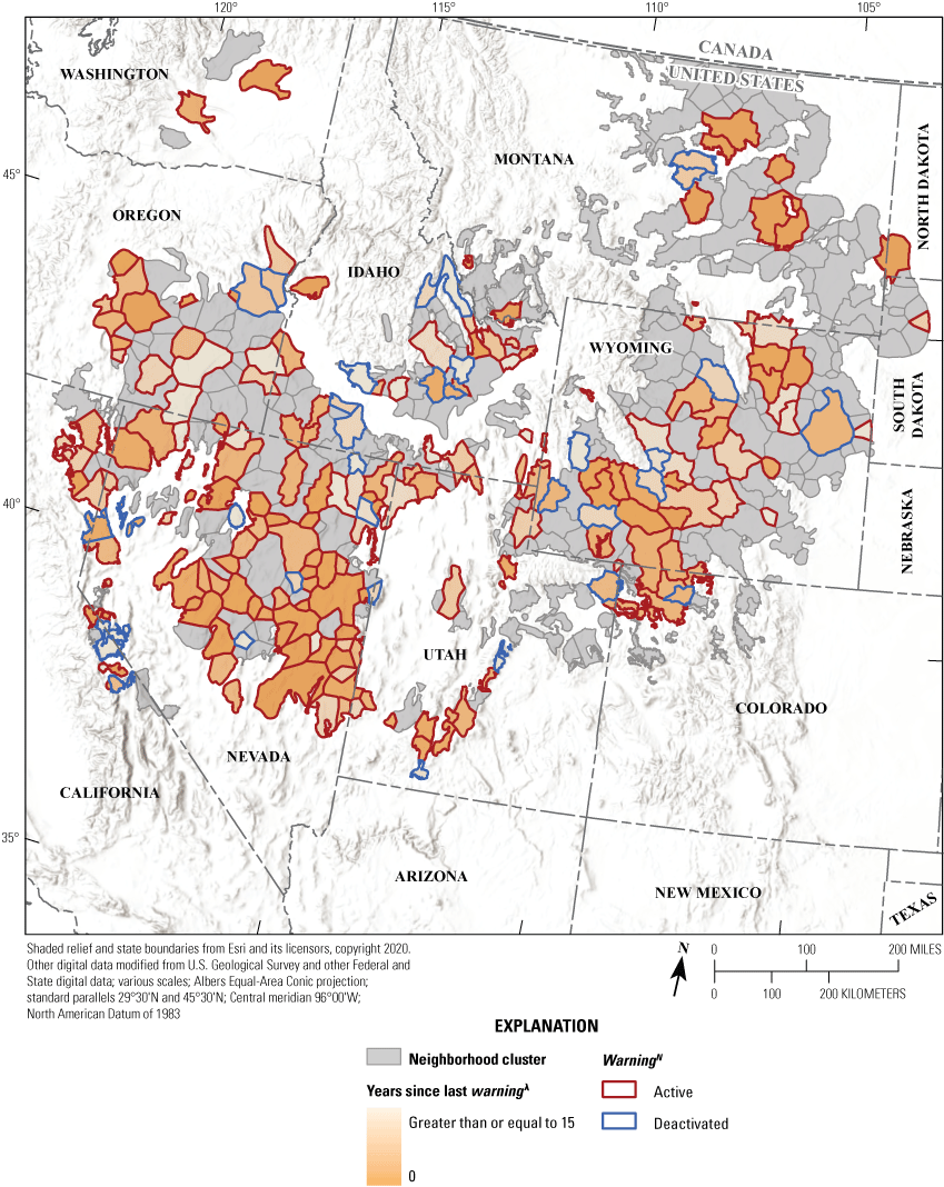
Spatial depiction of range-wide warnings (acute [warningλ] and chronic [warningN]) of greater sage-grouse (Centrocercus urophasianus) population declines at the neighborhood cluster scale in the western United States from 1990 to 2024. Polygon fill colors depict the number of elapsed years since the most recent warningλ. Polygon border colors depict if a neighborhood cluster recouped abundance losses following a warningλ (blue=yes, red=no), resulting in the deactivation of a chronic warning (warningN).
References Cited
Bureau of Land Management, 2015, Notice of availability of the record of decision and approved resource management plan amendments for the Great Basin Region greater sage-grouse sub-regions of Idaho and southwestern Montana; Nevada and northeastern California; Oregon; and Utah: Federal Register, v. 80, no. 185, p. 57633–57635, accessed August 15, 2022, at https://www.federalregister.gov/documents/2015/09/24/2015-24213/notice-of-availability-of-the-record-of-decision-and-approved-resource-management-plan -amendm.
Coates, P.S., Prochazka, B.G., Aldridge, C.L., O’Donnell, M.S., Edmunds, D.R., Monroe, A.P., Hanser, S.E., Wiechman, L.A., and Chenaille, M.P., 2022a, Range-wide population trend analysis for greater sage-grouse (Centrocercus urophasianus)—Updated 1960–2021: U.S. Geological Survey Data Report 1165, 16 p., accessed March 20, 2022, at https://doi.org/10.3133/dr1165.
Coates, P.S., Prochazka, B.G., Aldridge, C.L., O'Donnell, M.S., Edmunds, D.R., Monroe, A.P., Hanser, S.E., Wiechman, L.A., and Chenaille, M.P., 2022b, Trends and a targeted annual warning system for greater sage-grouse in the western United States (ver. 4.0, November 2025): U.S. Geological Survey data release. [Available at https://doi.org/10.5066/P9OQWGIV.]
Coates, P.S., Prochazka, B.G., O’Donnell, M.S., Aldridge, C.L., Edmunds, D.R., Monroe, A.P., Ricca, M.A., Wann, G.T., Hanser, S.E., Wiechman, L.A., and Chenaille, M.P., 2021, Range-wide greater sage-grouse hierarchical monitoring framework—Implications for defining population boundaries, trend estimation, and a targeted annual warning system: U.S. Geological Survey Open-File Report 2020–1154, 243 p., accessed August 15, 2022, at https://doi.org/10.3133/ofr20201154.
Dinkins, J.B., Lawson, K.J., and Beck, J.L., 2021, Influence of environmental change, harvest exposure, and human disturbance on population trends of greater sage-grouse: PLoS One, v. 16, no. 9, 29 p. [Available at https://doi.org/10.1371/journal.pone.0257198.]
Garton, E.O., Connelly, J.W., Horne, J.S., Hagen, C.A., Moser, A., and Schroeder, M.A., 2011, Greater sage-grouse population dynamics and probability of persistence, chap. 15 of Knick, S.T., and Connelly, J.W., eds., Greater sage-grouse—Ecology and conservation of a landscape species and its habitats: Berkeley, Calif., University of California Press, Studies in Avian Biology, v. 38, p. 292–381, accessed August 15, 2022, at https://doi.org/10.1525/california/9780520267114.003.0016.
Hanser, S.E., and Knick, S.T., 2011, Greater sage-grouse as an umbrella species for shrubland passerine birds—A multiscale assessment, chap. 19 of Knick, S.T., and Connelly, J.W., eds., Greater sage-grouse—Ecology and conservation of a landscape species and its habitats: Berkeley, Calif., University of California Press, Studies in Avian Biology, v. 38, p. 474–487, accessed August 15, 2022, at https://doi.org/10.1525/california/9780520267114.003.0020.
Miller, R.F., Knick, S.T., Pyke, D.A., Meinke, C.W., Hanser, S.E., Wisdom, M.J., and Hild, A.L., 2011, Characteristics of sagebrush habitats and limitations to long-term conservation, chap. 10 of Knick, S.T., and Connelly, J.W., eds., Greater sage-grouse—Ecology and conservation of a landscape species and its habitats: Berkeley, Calif., University of California Press, Studies in Avian Biology, v. 38, p. 144–184, accessed August 15, 2022, at https://doi.org/10.1525/california/9780520267114.003.0011.
O’Donnell, M.S., Edmunds, D.R., Aldridge, C.L., Heinrichs, J.A., Monroe, A.P., Coates, P.S., Prochazka, B.G., Hanser, S.E., Wiechman, L.A., Christiansen, T.J., Cook, A.A., Espinosa, S.P., Foster, L.J., Griffin, K.A., Kolar, J.L., Miller, K.S., Moser, A.M., Remington, T.E., Runia, T.J., Schreiber, L.A., Schroeder, M.A., Stiver, S.J., Whitford, N.I., and Wightman, C.S., 2021, Synthesizing and analyzing long-term monitoring data—A greater sage-grouse case study: Ecological Informatics, v. 63, 16 p. [Available at https://doi.org/10.1016/j.ecoinf.2021.101327.]
O’Donnell, M.S., Edmunds, D.R., Aldridge, C.L., Heinrichs, J.A., Monroe, A.P., Coates, P.S., Prochazka, B.G., Hanser, S.E., and Wiechman, L.A., 2022, Defining biologically relevant and hierarchically nested population units to inform wildlife management: Ecology and Evolution, v. 12, no. 12, 22 p. [Available at https://doi.org/10.1002/ece3.9565.]
Prochazka, B.G., Coates, P.S., Aldridge, C.L., O’Donnell, M.S., Edmunds, D.R., Monroe, A.P., Hanser, S.E., Wiechman, L.A., and Chenaille, M.P., 2024, Range-wide population trend analysis for greater sage-grouse (Centrocercus urophasianus)—Updated 1960–2023 (ver. 1.1, April 2024): U.S. Geological Survey Data Report 1190, 18 p., accessed May 20, 2024, at https://doi.org/10.3133/dr1190.
Prochazka, B.G., Coates, P.S., O’Donnell, M.S., Edmunds, D.R., Monroe, A.P., Ricca, M.A., Wann, G.T., Hanser, S.E., Wiechman, L.A., Doherty, K.E., Chenaille, M.P., and Aldridge, C.L., 2023, A targeted annual warning system developed for the conservation of a sagebrush indicator species: Ecological Indicators, v. 148, 13 p. [Available at https://doi.org/10.1016/j.ecolind.2023.110097.]
Remington, T.E., Welty, J.L., Aldridge, C.L., Jakes, A.F., Pilliod, D.S., Rachlow, J.L., and Smith, I.T., 2021, Sage-grouse management as an umbrella for conservation of sagebrush, chap. Q of Remington, T.E., Deibert, P.A., Hanser, S.E., Davis, D.M., Robb, L.A., and Welty, J.L., eds., Sagebrush conservation strategy—Challenges to sagebrush conservation: U.S. Geological Survey Open-File Report 2020–1125, p. 193–202, accessed May 27, 2025, at https://doi.org/10.3133/ofr20201125.
Rich, T.D., Wisdom, M.J., and Saab, V.A., 2005, Conservation of sagebrush steppe birds in the interior Columbia Basin, General Technical Report PSW-GTR-191, in Ralph, C.J., Rich, T., and Long, L., eds., Proceedings of the Third International Partners in Flight Conference: Albany, Calif., Department of Agriculture, Forest Service, Pacific Southwest Research Station, p. 589–606. [Available at https://www.fs.usda.gov/psw/publications/documents/psw_gtr191/psw_gtr191_0589-0606_rich.pdf.]
Rowland, M.M., Wisdom, M.J., Suring, L.H., and Meinke, C.W., 2006, Greater sage-grouse as an umbrella species for sagebrush-associated vertebrates: Biological Conservation, v. 129, no. 3, p. 323–335, accessed August 15, 2022, at https://doi.org/10.1016/j.biocon.2005.10.048.
Schroeder, M.A., Aldridge, C.L., Apa, A.D., Bohne, J.R., Braun, C.E., Bunnell, S.D., Connelly, J.W., Deibert, P.A., Gardner, S.C., Hilliard, M.A., Kobriger, G.D., McAdam, S.M., McCarthy, C.W., McCarthy, J.J., Mitchell, D.L., Rickerson, E.V., and Stiver, S.J., 2004, Distribution of sage-grouse in North America: The Condor, v. 106, no. 2, p. 363–376, accessed August 15, 2022, at https://doi.org/10.1093/condor/106.2.363.
U.S. Department of Agriculture Forest Service, 2015a, Notice of availability of the record of decision and approved land management plan amendments for the Great Basin Region greater sage-grouse sub-regions of Idaho and southwestern Montana; Nevada and Utah: Federal Register, v. 80, p. 57333–57334, accessed August 15, 2022, at https://www.federalregister.gov/documents/2015/09/23/2015-24169/notice-of-availability-of-the-record-of-decision-and-approved-land-management-plan-ame ndments.
U.S. Department of Agriculture Forest Service, 2015b, Notice of availability of the record of decision and approved land management plan amendments for the Rocky Mountain Region greater sage-grouse sub-regions northwest Colorado and Wyoming: Federal Register, v. 80, p. 57332–57333, accessed August 15, 2022, at https://www.federalregister.gov/documents/2015/09/23/2015-24168/notice-of-availability-of-the-record-of-decision-and-approved-land-management-plan-ame ndments-fo.
U.S. Fish and Wildlife Service, 2015, Endangered and threatened wildlife and plants; 12-month finding on a petition to list greater sage-grouse (Centrocercus urophasianus) as an endangered or threatened species: Federal Register, v. 80, no. 191, p. 59857–59942, accessed August 15, 2022, at https://www.govinfo.gov/content/pkg/FR-2015-10-02/pdf/2015-24292.pdf.
Western Association of Fish and Wildlife Agencies, 2015, Greater sage-grouse population trends—An analysis of lek count databases 1965–2015: Cheyenne, Wyo., Western Association of Fish and Wildlife Agencies, 55 p., accessed August 15, 2022, at https://ir.library.oregonstate.edu/concern/technical_reports/ng451p621.
Glossary
- Abundance index
An index based on the ratio of apparent abundance relative to the mean apparent abundance calculated across all years of data used in the analysis (for example, 1960–2024).
- Apparent abundance
Greater sage-grouse population data are collected at leks, and birds are counted yearly in the spring. These counts do not account for non-visiting/non-detection of individuals and exclude females (only males are used in our models). Therefore, the data used in models are considered as apparent abundance versus actual abundance (for example, data collected from a census design).
- Climate cluster (CC)
Large regions of the landscape that group leks with similar climate conditions (https://doi.org/10.3133/ofr20201154). Neighborhood clusters are nested within climate clusters. Climate clusters are level 13 of the spatial clusters.
- Cluster
Nested management units that are defined by sage-grouse biology. There are 13 nested scales, or levels, to support management at regional (coarse) to local (fine) scales.
- Credible interval (CRI)
Similar to confidence intervals (CI) used in frequentist statistics (confidence an estimated value indicates a true value), these characterize the probability of an unobserved parameter occurring within the specified distribution.
- Cycle
The temporal range that is repeating a pattern. It represents a single oscillation and is measured nadir to nadir.
- Extirpation probability
The probability that, given current population trends, a population will be reduced to less than two males, which aligns with State wildlife agencies definition of lek inactivity. Extirpation probabilities are calculated at three temporal scales: two, four, and six cycles into the future.
- Fast signal
A fast signal indicates a population is declining, and the rate of decline is steeply decoupled from the regional trend.
- Intrinsic growth rate
The rate at which a population increases without being affected by density dependence or interspecific competition (for example, potential reproductivity capacity).
- Lambda
The finite rate of change for a population over a specified period. For example, the ratio of population size at the end of one interval (defined as nadir) to the population size at the end of the previous interval.
- Nadir
The location within a single, complete population oscillation that has the lowest abundance.
- Neighborhood cluster (NC)
Polygons that group leks based on their connectivity (https://doi.org/10.1111/2041-210X.13949) and represent closed population units. Connectivity is upheld if (1) leks are less than 30 kilometers (km) apart; and (2) lek connections do not cross high traffic volumes on interstates, highways, and primary roads (greater than or equal to 4,000 annual average daily traffic). Neighborhood clusters contain approximately 20–30 leks. Less than 20 leks occur because there are too few leks to merge with a connected neighboring cluster or because a rule prevents the connection. Neighborhood clusters are level 2 of the spatial clusters.
- Oscillation
A phenomenon where populations experience natural, regular fluctuations in abundance. In sage-grouse, these oscillations are driven by climatic factors such as precipitation that mediate vegetation used for food, nesting, and brood rearing.
- Posterior distribution
A probability distribution reflecting updated estimates of the unobserved parameter (for example, rate of population change) given the observed data (male counts at leks). This is a conditional distribution of the unobserved parameter given the observed data.
- Prior distribution
A probability distribution representing the uncertainty about a parameter before any data are observed.
- Signal
A signal is assigned to a population that is (1) declining at a local scale (lek or neighborhood cluster); (2) is decoupled from the trend at the regional scale (climate cluster); and (3) the decline is sustained over multiple years.
- Slow signal
A slow signal indicates a population is declining, and the rate of decline is slightly decoupled from the regional trend.
- Targeted Annual Warning System (TAWS)
A system that identifies sustained, aberrant population declines across nested spatial scales on an annual basis. To determine if a decline is aberrant, the TAWS compares the rate of population change at a local scale (leks or neighborhood clusters) to the rate of population change at a regional scale (climate cluster). In this way, the TAWS helps managers differentiate between broad-scale, natural population declines driven by climatic factors that are difficult to manage and unexpected population declines driven by local factors that may be mitigated through management.
- Trend
The estimated change in population performance, or abundance, over some period. In this analysis, periods are defined as one, two, three, four, five, or six cycles. Estimates within and across cycles are made nadir-to-nadir to avoid overestimating population performance.
- Warning
Assigned to populations that had slow signals in 3 out of 4 consecutive years or fast signals in 2 out of 3 consecutive years.
- Watch
Assigned to populations that had slow signals over 2 consecutive years.
Abbreviations
estimated apparent abundance
estimated intrinsic rate of population change
estimated finite rate of population change
BLM
Bureau of Land Management
CC
climate cluster
CRI
credible interval
NC
neighborhood cluster
QA/QC
quality assessment and quality control
SD
standard deviation
SSM
state-space model
TAWS
targeted annual warning system
USGS
U.S. Geological Survey
For more information concerning the research in this report, contact the
Director, Western Ecological Research Center
U.S. Geological Survey
3020 State University Drive East
Sacramento, California 95819
https://www.usgs.gov/centers/werc
Publishing support provided by the USGS Science Publishing Network,
Sacramento Publishing Service Center
Disclaimers
Any use of trade, firm, or product names is for descriptive purposes only and does not imply endorsement by the U.S. Government.
Although this information product, for the most part, is in the public domain, it also may contain copyrighted materials as noted in the text. Permission to reproduce copyrighted items must be secured from the copyright owner.
Suggested Citation
Prochazka, B.G., Coates, P.S., Aldridge, C.L., O'Donnell, M.S., Edmunds, D.R., Monroe, A.P., Hanser, S.E., Wiechman, L.A., and Chenaille, M.P., 2025, Range-wide population trend analysis for greater sage-grouse (Centrocercus urophasianus)—Updated 1960–2024: U.S. Geological Survey Data Report 1217, 22 p., https://doi.org/10.3133/dr1217.
ISSN: 2771-9448 (online)
Study Area
| Publication type | Report |
|---|---|
| Publication Subtype | USGS Numbered Series |
| Title | Range-wide population trend analysis for greater sage-grouse (Centrocercus urophasianus)—Updated 1960–2024 |
| Series title | Data Report |
| Series number | 1217 |
| DOI | 10.3133/dr1217 |
| Publication Date | December 01, 2025 |
| Year Published | 2025 |
| Language | English |
| Publisher | U.S. Geological Survey |
| Publisher location | Reston, VA |
| Contributing office(s) | Western Ecological Research Center |
| Description | Report: viii, 22 p.; Data Release |
| Country | United States |
| State | California, Colorado, Idaho, Montana, Nevada, North Dakota, Oregon, South Dakota, Utah, Washington, Wyoming |
| Online Only (Y/N) | Y |