

System Characterization Report on Tanager
Links
- Document: Report (9.87 MB pdf) , HTML , XML
- Larger Work: This publication is Chapter W of System characterization of Earth observation sensors
- Dataset: Planet Labs PBC dataset - Tanager—Cutting-edge hyperspectral from orbit
- Version History: Version history (txt)
- Download citation as: RIS | Dublin Core
Executive Summary
This report addresses the system characterization of the Tanager satellite hyperspectral sensor created by Planet Labs PBC and is part of a series of system characterization reports produced and delivered by the U.S. Geological Survey Earth Resources Observation and Science Cal/Val Center of Excellence. These reports present and detail the methodology and procedures for characterization; present technical and operational information about the Tanager hyperspectral sensor; and provide a summary of test measurements, data retention practices, data analysis results, and conclusions.
This report summarizes the sensor performance of the Tanager based on the U.S. Geological Survey Earth Resources Observation and Science Cal/Val Center of Excellence system characterization process. In summary, we determined that the Tanager exhibits a band-to-band geometric error ranging from −0.074 to 0.097 pixel. Compared to the Landsat Operational Land Imager, geometric offsets ranged from −5.980 meters (−0.20 pixel) to 11.348 meters (0.40 pixel). Radiometric comparisons showed offsets between −0.004 and 0.056 with slopes from 0.830 to 1.066. Spectral shifts are found between 0.65 and 0.75 nanometers. Finally, spatial performance evaluation yielded a point spread function full width at half maximum of 1.27 to 1.75 pixels, a relative edge response of 0.802 to 0.651, and a modulation transfer function at Nyquist of 0.488 to 0.253.
Introduction
This report addresses the system characterization of the Tanager satellite hyperspectral sensor created by Planet Labs PBC and is part of a series of system characterization reports produced and delivered by the U.S. Geological Survey (USGS) Earth Resources Observation and Science Cal/Val Center of Excellence. These reports present and detail the methodology and procedures for characterization; present technical and operational information about the Tanager hyperspectral sensor; and provide a summary of test measurements, data retention practices, data analysis results, and conclusions.
The Planet Labs PBC Tanager is a hyperspectral electro-optical instrumentation designed to deliver imagery across the visible and shortwave infrared regions. The Tanager supports a broad spectrum of applications, but its core mission is to detect and mitigate methane emissions across the globe. The Tanager is able to map facility-scale methane emissions to enhance leak detection and repair efforts (Planet Labs PBC, 2026).
The data analysis results provided within this report have been derived from approved Joint Agency Commercial Imagery Evaluation (JACIE) processes and procedures (Cantrell and Christopherson, 2024). The JACIE was formed to leverage resources from several Federal agencies for the characterization of remote sensing data and to share those results across the remote sensing community. More information about JACIE is available at https://www.usgs.gov/calval/jacie.
The purpose of this report is to describe the Tanager hyperspectral sensor, test its performance in B2B, I2I, radiometric, and spatial, complete related data analyses to quantify these performances, and report the results in a standardized document. In this chapter, the Tanager hyperspectral sensor is described. The performance testing of the system involved geometric, radiometric, and spatial analyses. The scope of the geometric analysis is limited to testing the interior alignments of spectral bands against each other, and the exterior alignment is tested in reference to the Landsat Operational Land Imager (OLI; U.S. Geological Survey, 2025).
The USGS Earth Resources Observation and Science Cal/Val Center of Excellence (ECCOE; U.S. Geological Survey, 2020) and the associated system characterization process used for this assessment follow the USGS Fundamental Science Practices, which include maintaining data, information, and documentation needed to reproduce and validate the scientific analysis documented in this report. Additional information and guidance about Fundamental Science Practices and related resource information of interest to the public are available at https://www.usgs.gov/about/organization/science-support/office-science-quality-and-integrity/fundamental-science-practices. For additional information related to the report, please contact ECCOE at [email protected].
System Description
This section describes the satellite and operational details and provides information about the Planet Labs PBC Tanager hyperspectral sensor. Hyperspectral data provide finer spectral signatures to be used for scientific analysis.
Satellite and Operational Details
The satellite and operational details for Tanager are listed in table 1.
Table 1.
Satellite and operational details for the Planet Labs PBC Tanager (Zandbergen and others, 2022; Duren and others, 2025; Keremedjiev and others, 2025; LeDuc and others, 2026; Planet Labs PBC, 2026).[km, kilometer; °, degree; ±, plus or minus;~, about; m, meter]
| Product information | Tanager |
|---|---|
| Sensor name(s) | Tanager-1 |
| Sensor type | Hyperspectral |
| Mission type | Global methane detection and land-monitoring mission |
| Launch date | August 16, 2024 |
| Expected lifetime | 5 years |
| Operating orbit | Sun-synchronous orbit |
| Orbital altitude range | 406–435 km |
| Sensor angle altitude | 97.4° inclination |
| Imaging time | 12:00 p.m. ± 1 hour (local time) |
| Geographic coverage | 18-km swath |
| Temporal resolution | ~7 days |
| Temporal coverage | 2024 to present (2026) |
| Imaging angles | ±30° |
| Ground sample distance(s) | 30–35 m |
| Product abstract | https://docs.planet.com/data/imagery/tanager/ |
Sensor Information
The imaging sensor details for Tanager are listed in table 2. The spectral resolution of each band is 5 nanometers (nm) for full width at half maximum (FWHM).
Table 2.
Imaging sensor details for the Planet Labs PBC Tanager (Zandbergen and others, 2022; Duren and others, 2025; Keremedjiev and others, 2025; LeDuc and others, 2026; Planet Labs PBC, 2026).[F-number, ratio of a lens focal length to its aperture diameter; °, degree; km, kilometer; nm, nanometer; m, meter]
Procedures
The ECCOE has established standard processes to identify Earth observing systems of interest and to assess the geometric and radiometric qualities of data products from these systems (Cantrell and Christopherson, 2024).
The assessment steps are as follows:
-
1. System identification and investigation to learn the general specifications of the satellite and its sensor(s);
-
2. Data receipt and initial inspection to understand the characteristics and any overt flaws in the data product so that it may be further analyzed;
-
3. Geometric characterization, including interior geometric orientation measuring the relative alignment of spectral bands and exterior geometric orientation measuring how well the georeferenced pixels within the image are aligned to a known reference; and
-
4. Radiometric characterization, including assessing how well the data product correlates with a known reference and, when possible, assessing the signal-to-noise ratio.
-
• Correction of defective pixels that cause dark striping;
-
• Spectral resampling of hyperspectral data to match the spectral response function of Landsat OLI; and
-
• Computation of solar irradiance by resampling high-resolution extraterrestrial solar irradiance based on the spectral response function of Landsat OLI.
Measurements
The observed USGS measurements are listed in table 3. Details about the methodologies used are outlined in the “Analysis” section.
Table 3.
U.S. Geological Survey measurement results for the Planet Labs PBC Tanager.[nm, nanometer; RMSE, root mean square error; OLI, Operational Land Imager; m, meter; R2, coefficient of determination; %, percent; RER, relative edge response; FWHM, full width at half maximum; MTF, modulation transfer function]
Analysis
This section of the report describes the geometric and radiometric performance of the Tanager hyperspectral sensor.
Geometric Performance
The geometric performance for the Tanager sensor is characterized in terms of the band-to-band alignment and image-to-image relative geometric accuracy.
Band to Band
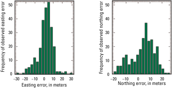
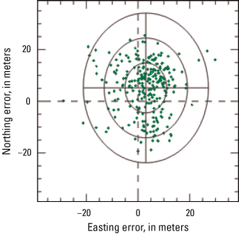
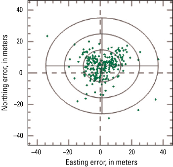
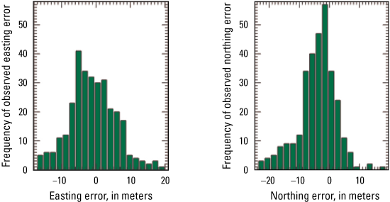
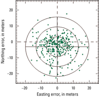
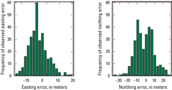
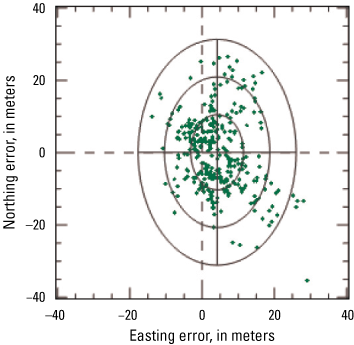
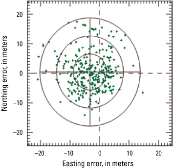
For this analysis, each band of the Tanager imagery was registered against one reference band (band 38 at 561 nm). Scene identifiers for all band-to-band scenes discussed in this report are provided in table 4. Scene identifier 20250405_190836_16_4001 shows part of the Mojave Desert in Arizona and was used as an example image to compute band-to-band error. The grid system and error vectors for band 22 are shown in figure 1. The red arrows show the relative error vector for each yellow grid, with x and y vector components representing the easting and northing error, respectively. Grids with missing arrows represent the outliers. Also, the scatterplot of the easting-northing error shows a distribution with three circles representing one, two, and three standard deviations.
Table 4.
Summary of band-to-band scene results using band 38 as a reference (in pixels).[ID, identifier; RMSE, root mean square error]
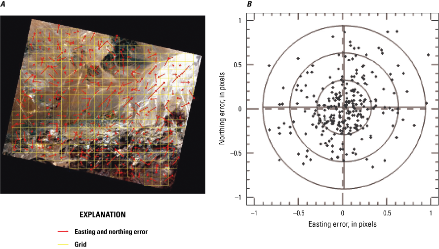
The Mojave Desert, Arizona, Planet Labs PBC Tanager scene (20250405_190836_16_4001) used to compute band-to-band error. A, image of grid showing band-to-band geometric error map of band 22 (481 nanometers) using band 38 (561 nanometers) as reference; B, the error vector scatterplot. Image copyrighted by Planet Labs PBC, licensed under the Creative Commons Attribution-NonCommercial-ShareAlike 2.0 Generic license.
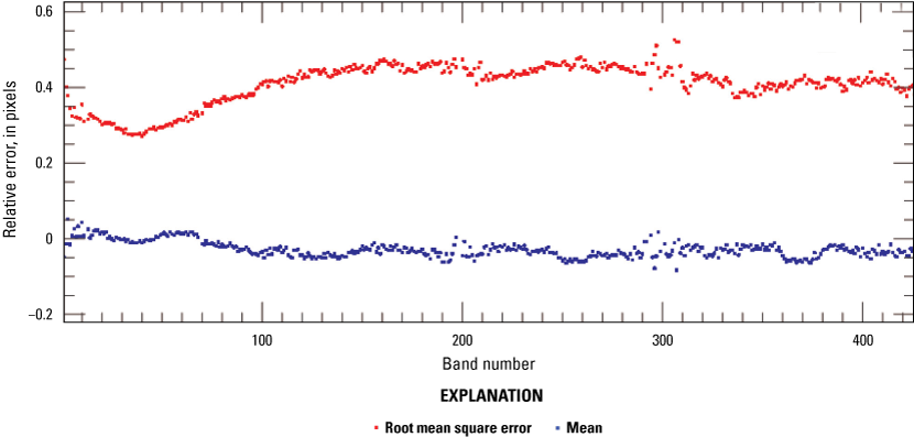
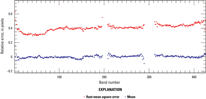
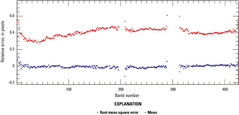
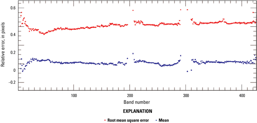
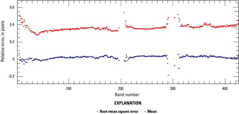
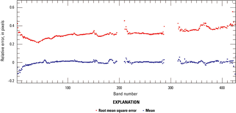
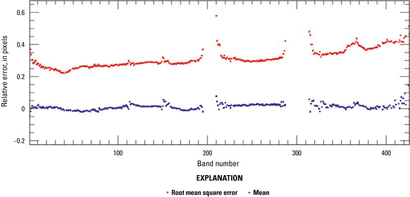
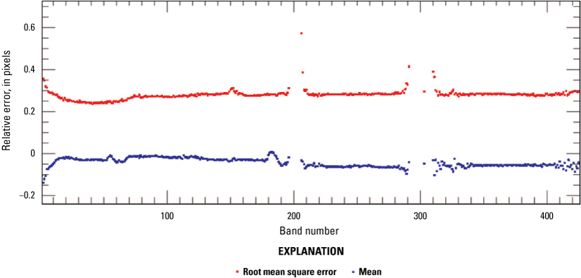
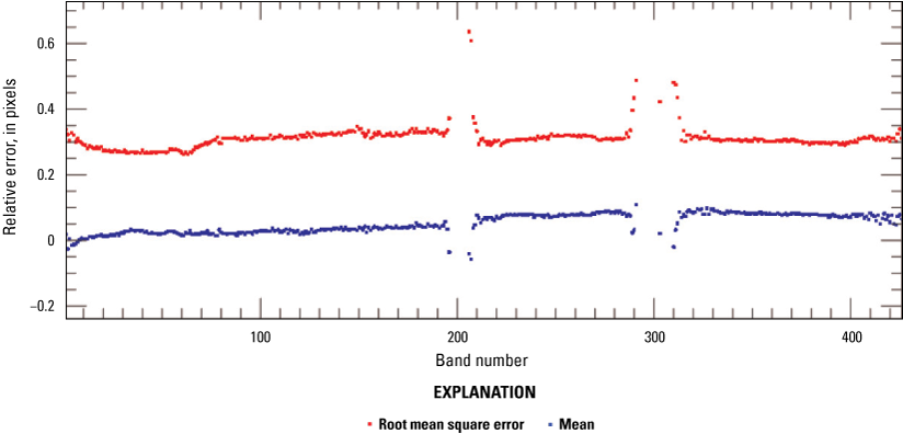
For the Mojave Desert scene, the mean difference and root mean square error values for the easting direction are shown in figure 2, and those values for the northing direction are shown in figure 3. Similarly, figures 4 and 5 are band-to-band results for the Indian Tanager scene (20250420_060625_00_4001). The band-to-band results for the Sudanese Tanager scene (20250502_090330_87_4001) are shown in figures 6 and 7. The band-to-band results for the Australian Tanager scene (20250305_010639_32_4001) are shown in figures 8 and 9. The band-to-band results for the Chinese Tanager scene (20250523_055213_30_4001) are shown in figures 10 and 11. The band-to-band results of all five scenes are summarized in table 4, where the erroneous values near the water vapor bands were not included in the result range summary in table 4.
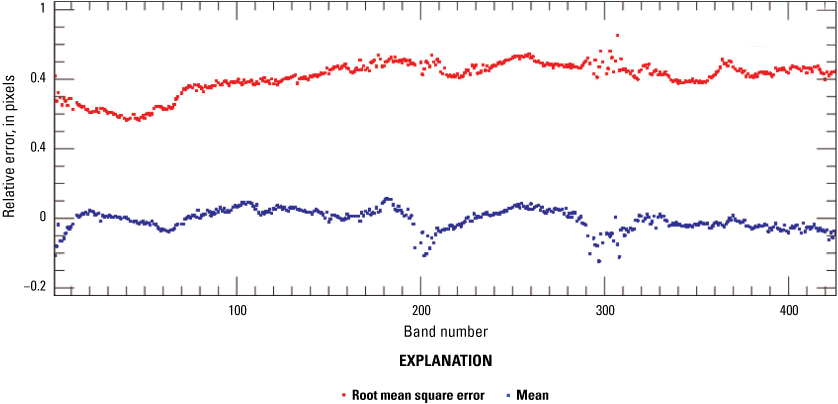
Graph showing relative band-to-band easting geometric error derived from the Mojave Desert, Arizona, Planet Labs PBC Tanager scene (20250405_190836_16_4001) using band 38 as a reference.
Graph showing relative band-to-band northing geometric error derived from the Mojave Desert, Arizona, Planet Labs PBC Tanager scene (20250405_190836_16_4001) using band 38 as a reference.
Graph showing relative band-to-band easting geometric error derived from the Indian Planet Labs PBC Tanager scene (20250420_060625_00_4001) using band 38 as a reference.
Graph showing relative band-to-band northing geometric error derived from the Indian Planet Labs PBC Tanager scene (20250420_060625_00_4001) using band 38 as a reference.
Graph showing relative band-to-band easting geometric error derived from the Sudanese Planet Labs PBC Tanager scene (20250502_090330_87_4001) using band 38 as a reference.
Graph showing relative band-to-band northing geometric error derived from the Sudanese Planet Labs PBC Tanager scene (20250502_090330_87_4001) using band 38 as a reference.
Graph showing relative band-to-band easting geometric error derived from the Australian Planet Labs PBC Tanager scene (20250305_010639_32_4001) using band 38 as a reference.
Graph showing relative band-to-band northing geometric error derived from the Australian Planet Labs PBC Tanager scene (20250305_010639_32_4001) using band 38 as a reference.
Graph showing relative band-to-band easting geometric error derived from the Chinese Planet Labs PBC Tanager scene (20250523_055213_30_4001) using band 38 as a reference.
Graph showing relative band-to-band northing geometric error derived from the Chinese Planet Labs PBC Tanager scene (20250523_055213_30_4001) using band 38 as a reference.
Image to Image
For this analysis, spectrally resampled Tanager reflectance (ρi), where the subscript i represents the i-th Landsat OLI band, was used. The spectral resampling of Tanager hyperspectral reflectance, ρTanager(λ), where λ denotes wavelength, is performed using the Landsat OLI spectral response function, ℜOLI_i(λ) (Barsi and others, 2014).
Six Tanager-Landsat OLI scene pairs were used for image-to-image analysis. A normalized cross-correlation matrix was computed, and its local maxima with subpixel analysis were determined to estimate the mean error and root mean square error results shown in table 5 and represented in pixels at a 30-meter (m) ground sample distance (GSD).
Table 5.
Geometric error of the Planet Labs PBC Tanager relative to Landsat Operational Land Imager.[OLI, Operational Land Imager; ID, identifier; RMSE, root mean square error; m, meter]
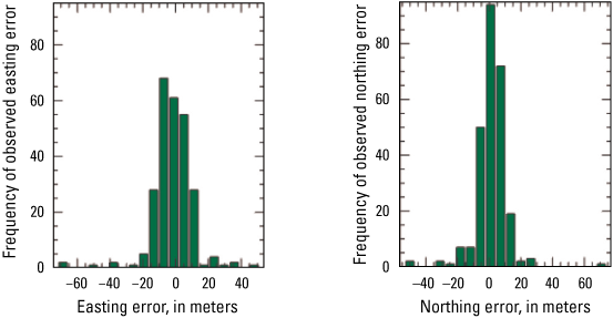
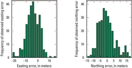
For each of the six Tanager images, geometric error maps illustrating the directional shift and relative magnitude of the shift, when compared with Landsat OLI, are provided in figures 12 through 29.
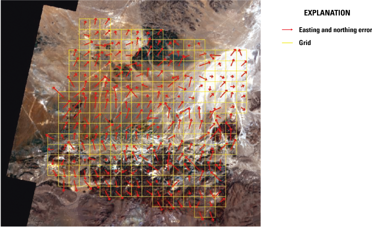
Image-to-image geometric error map with error vector for each grid using the Mojave Desert, Arizona, scene pair comprising a Planet Labs PBC Tanager scene (20250405_190836_16_4001) and a Landsat Operational Land Imager scene (LC08_L1TP_040035_20250405_20250412_02_T1). Tanager image copyrighted by Planet Labs PBC, licensed under the Creative Commons Attribution-NonCommercial-ShareAlike 2.0 Generic license. Landsat image by U.S. Geological Survey.
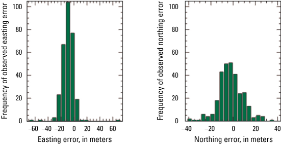
Histogram of image-to-image geometric error derived from the Mojave Desert, Arizona, scene pair comprising a Planet Labs PBC Tanager scene (20250405_190836_16_4001) and a Landsat Operational Land Imager scene (LC08_L1TP_040035_20250405_20250412_02_T1).
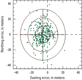
Error scatterplot of image-to-image geometric error derived from the Mojave Desert, Arizona, scene pair comprising a Planet Labs PBC Tanager scene (20250405_190836_16_4001) and a Landsat Operational Land Imager scene (LC08_L1TP_040035_20250405_20250412_02_T1).
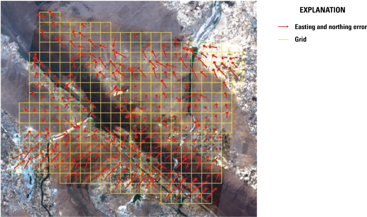
Image-to-image geometric error map with error vector for each grid derived from the Indian scene pair comprising a Planet Labs PBC Tanager scene (20250420_060625_00_4001) and a Landsat Operational Land Imager scene (LC09_L1TP_146043_20250420_20250420_02_T1). Tanager image copyrighted by Planet Labs PBC, licensed under the Creative Commons Attribution-NonCommercial-ShareAlike 2.0 Generic license. Landsat image by U.S. Geological Survey.
Histogram of image-to-image geometric derived from the Indian scene pair comprising a Planet Labs PBC Tanager scene (20250420_060625_00_4001) and a Landsat Operational Land Imager scene (LC09_L1TP_146043_20250420_20250420_02_T1).
Error scatterplot of image-to-image geometric error derived from the Indian scene pair comprising a Planet Labs PBC Tanager scene (20250420_060625_00_4001) and a Landsat Operational Land Imager scene (LC09_L1TP_146043_20250420_20250420_02_T1).
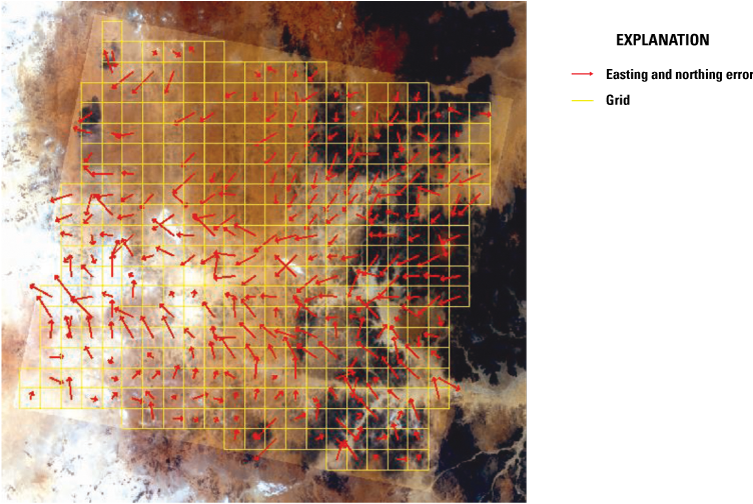
Image-to-image geometric error map with error vector for each grid derived from the Sudanese scene pair comprising a Planet Labs PBC Tanager scene (20250502_090330_87_4001) and a Landsat Operational Land Imager scene (LC08_L1TP_174049_20250502_20250508_02_T1). Tanager image copyrighted by Planet Labs PBC, licensed under the Creative Commons Attribution-NonCommercial-ShareAlike 2.0 Generic license. Landsat image by U.S. Geological Survey.
Histogram of image-to-image geometric error derived from the Sudanese scene pair comprising a Planet Labs PBC Tanager scene (20250502_090330_87_4001) and a Landsat Operational Land Imager scene (LC08_L1TP_174049_20250502_20250508_02_T1).
Error scatterplot of image-to-image geometric error derived from the Sudanese scene pair comprising a Planet Labs PBC Tanager scene (20250502_090330_87_4001) and a Landsat Operational Land Imager scene (LC08_L1TP_174049_20250502_20250508_02_T1).
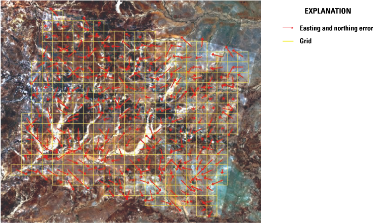
Image-to-image geometric error map with error vector for each grid derived from the Australian scene pair comprising a Planet Labs PBC Tanager scene (20250305_010639_32_4001) and a Landsat Operational Land Imager scene (LC09_L1TP_096076_20250305_20250305_02_T1). Tanager image copyrighted by Planet Labs PBC, licensed under the Creative Commons Attribution-NonCommercial-ShareAlike 2.0 Generic license. Landsat image by U.S. Geological Survey.
Histogram of image-to-image geometric error derived from the Australian scene pair comprising a Planet Labs PBC Tanager scene (20250305_010639_32_4001) and a Landsat Operational Land Imager scene (LC09_L1TP_096076_20250305_20250305_02_T1).
Error scatterplot of image-to-image geometric error derived from the Australian scene pair comprising a Planet Labs PBC Tanager scene (20250305_010639_32_4001) and a Landsat Operational Land Imager scene (LC09_L1TP_096076_20250305_20250305_02_T1).
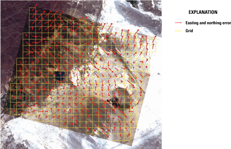
Image-to-image geometric error map with error vector for each grid derived from the Chinese scene pair comprising a Planet Labs PBC Tanager scene (20250523_055213_30_4001) and a Landsat Operational Land Imager scene (LC08_L1TP_145028_20250523_20250602_02_T1). Tanager image copyrighted by Planet Labs PBC, licensed under the Creative Commons Attribution-NonCommercial-ShareAlike 2.0 Generic license. Landsat image by U.S. Geological Survey.
Histogram of image-to-image geometric error derived from the Chinese scene pair comprising a Planet Labs PBC Tanager scene (20250523_055213_30_4001) and a Landsat Operational Land Imager scene (LC08_L1TP_145028_20250523_20250602_02_T1).
Error scatterplot of image-to-image geometric error derived from the Chinese scene pair comprising a Planet Labs PBC Tanager scene (20250523_055213_30_4001) and a Landsat Operational Land Imager scene (LC08_L1TP_145028_20250523_20250602_02_T1).
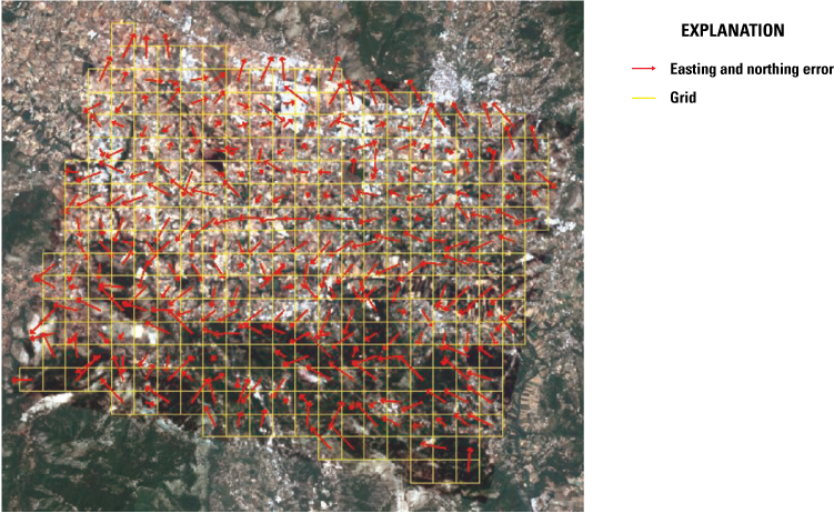
Image-to-image geometric error map with error vector for each grid derived from the Italian scene pair comprising a Planet Labs PBC Tanager scene (20250627_103759_58_4001) and a Landsat Operational Land Imager scene (LC09_L1TP_190031_20250627_20250627_02_T1). Tanager image copyrighted by Planet Labs PBC, licensed under the Creative Commons Attribution-NonCommercial-ShareAlike 2.0 Generic license. Landsat image by U.S. Geological Survey.
Histogram of image-to-image geometric error derived from the Italian scene pair comprising a Planet Labs PBC Tanager scene (20250627_103759_58_4001) and a Landsat Operational Land Imager scene (LC09_L1TP_190031_20250627_20250627_02_T1).
Error scatterplot of image-to-image geometric error derived from the Italian scene pair comprising a Planet Labs PBC Tanager scene (20250627_103759_58_4001) and a Landsat Operational Land Imager scene (LC09_L1TP_190031_20250627_20250627_02_T1).
Radiometric Performance
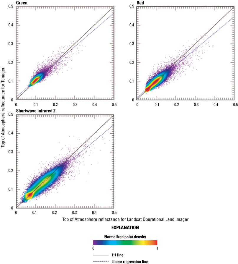
For this analysis, cloud-free regions of interest were selected within three near-coincident Tanager-Landsat OLI scene pairs. Top of Atmosphere reflectance (TOAR) comparison results are listed in table 6.
Table 6.
Top of Atmosphere reflectance comparison of the Planet Labs PBC Tanager and Landsat Operational Land Imager.[OLI, Operational Land Imager; ID, identifier; B, band; CA, coastal aerosol; NIR, near infrared; SW1, shortwave infrared 1; SW2, shortwave infrared 2; %, percent; R2, coefficient of determination]
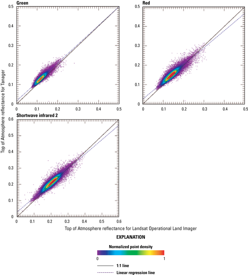
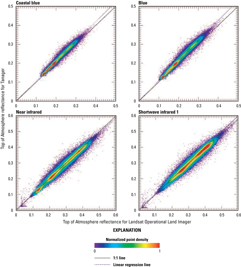
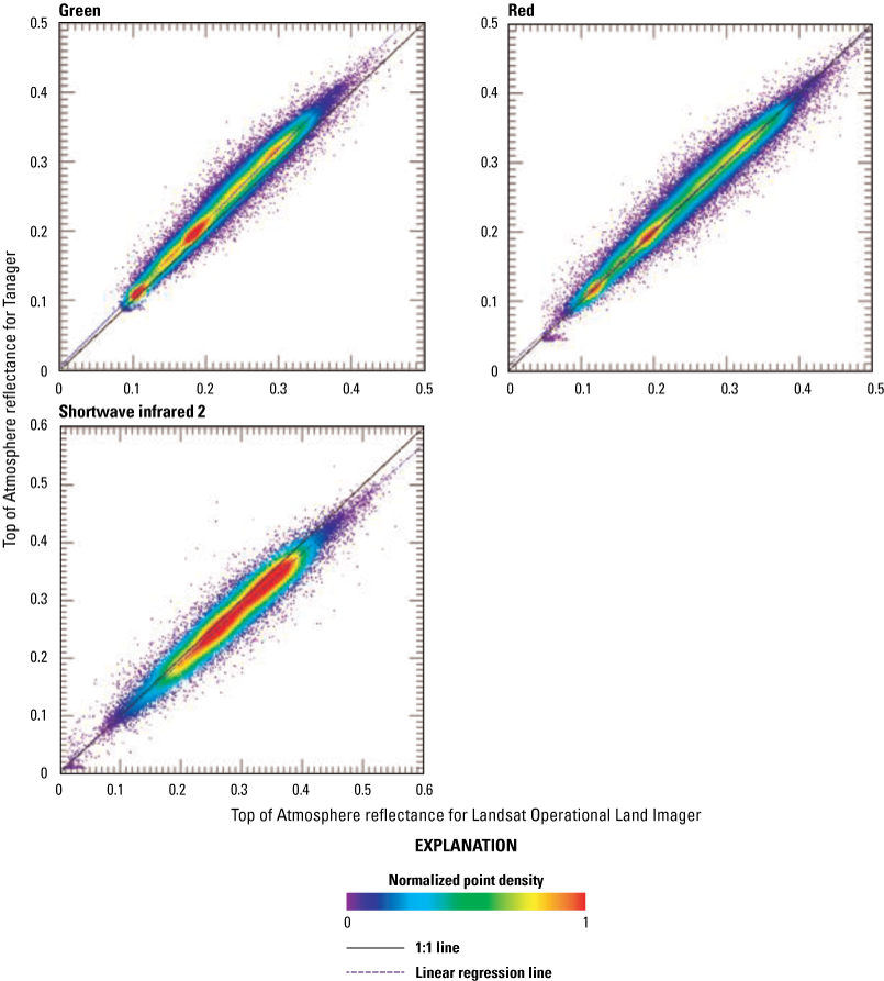
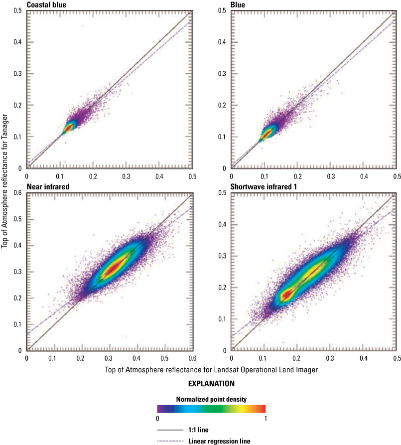
Once the relative georeferencing error between the Landsat OLI and Tanager has been corrected, TOAR values from the two sensors are extracted. The scatterplots shown in figures 30 through 35 are drawn in a way that the x-axis is the reference sensor (Landsat OLI) and the y-axis is the comparison sensor (Tanager). Ideally, the slope should be near unity (1.0) because it is spectrally resampled from hyperspectral data using spectral response of Landsat OLI, and the offset should be near zero. If the slope is greater than unity, that means Tanager tends to overestimate TOAR compared to Landsat OLI. A band-by-band graphical comparison of the Mojave Desert, Indian, Sudanese, Australian, Chinese, and Italian Tanager-Landsat OLI scene pairs is shown in figures 30 through 35.
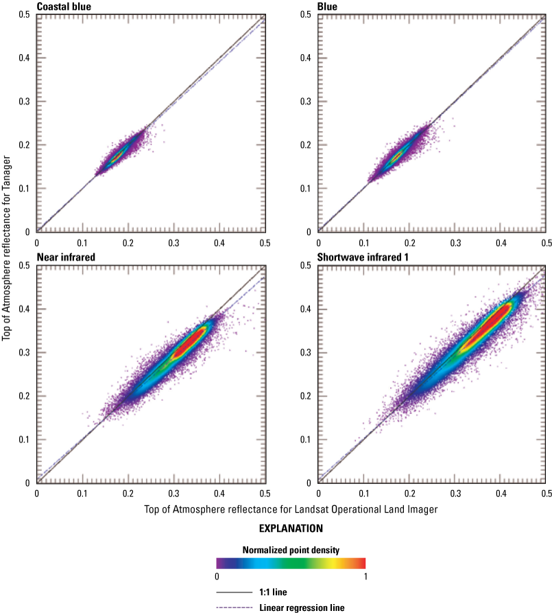
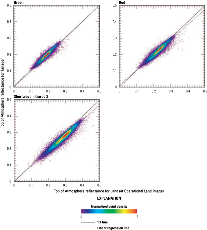
Radiometric scatterplots comparing Top of Atmosphere reflectance values derived from all seven bands of the spectrally resampled Mojave Desert, Arizona, Planet Labs PBC Tanager scene (20250405_190836_16_4001) and Landsat Operational Land Imager scene (LC08_L1TP_040035_20250405_20250412_02_T1).
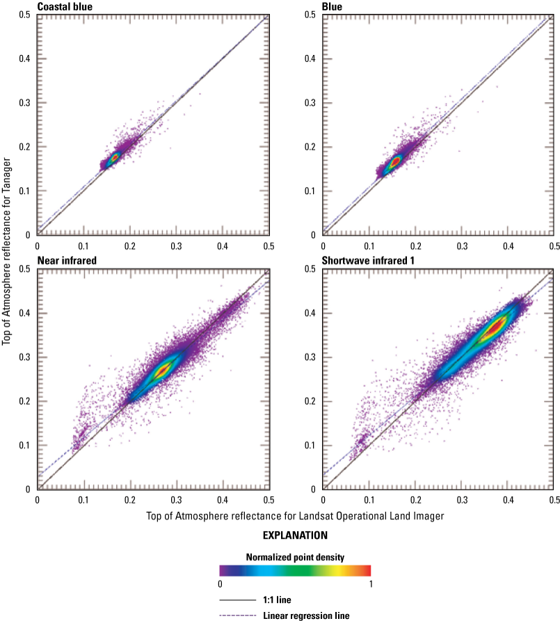
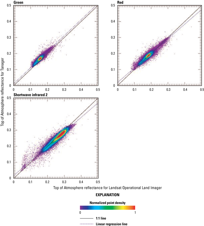
Radiometric scatterplots comparing Top of Atmosphere reflectance values derived from all seven bands of the spectrally resampled Indian Planet Labs PBC Tanager scene (20250420_060625_00_4001) and Landsat Operational Land Imager scene (LC09_L1TP_146043_20250420_20250420_02_T1).
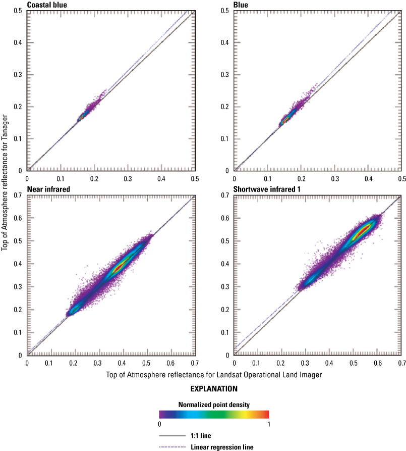
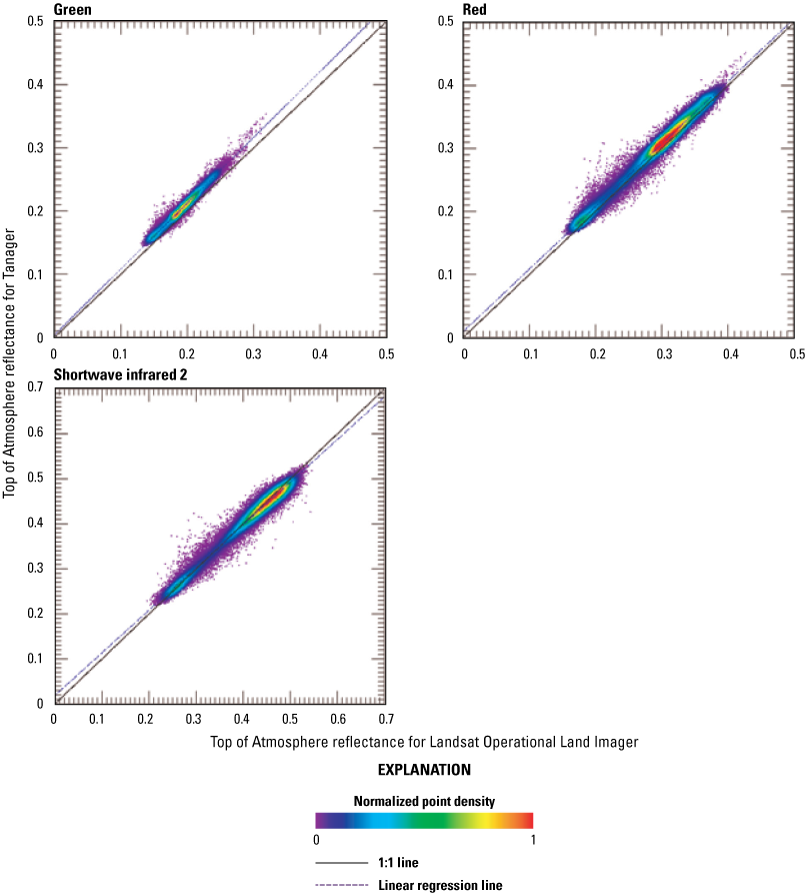
Radiometric scatterplots comparing Top of Atmosphere reflectance values derived from all seven bands of the spectrally resampled Sudanese Planet Labs PBC Tanager scene (20250502_090330_87_4001) and Landsat Operational Land Imager scene (LC08_L1TP_174049_20250502_20250508_02_T1).
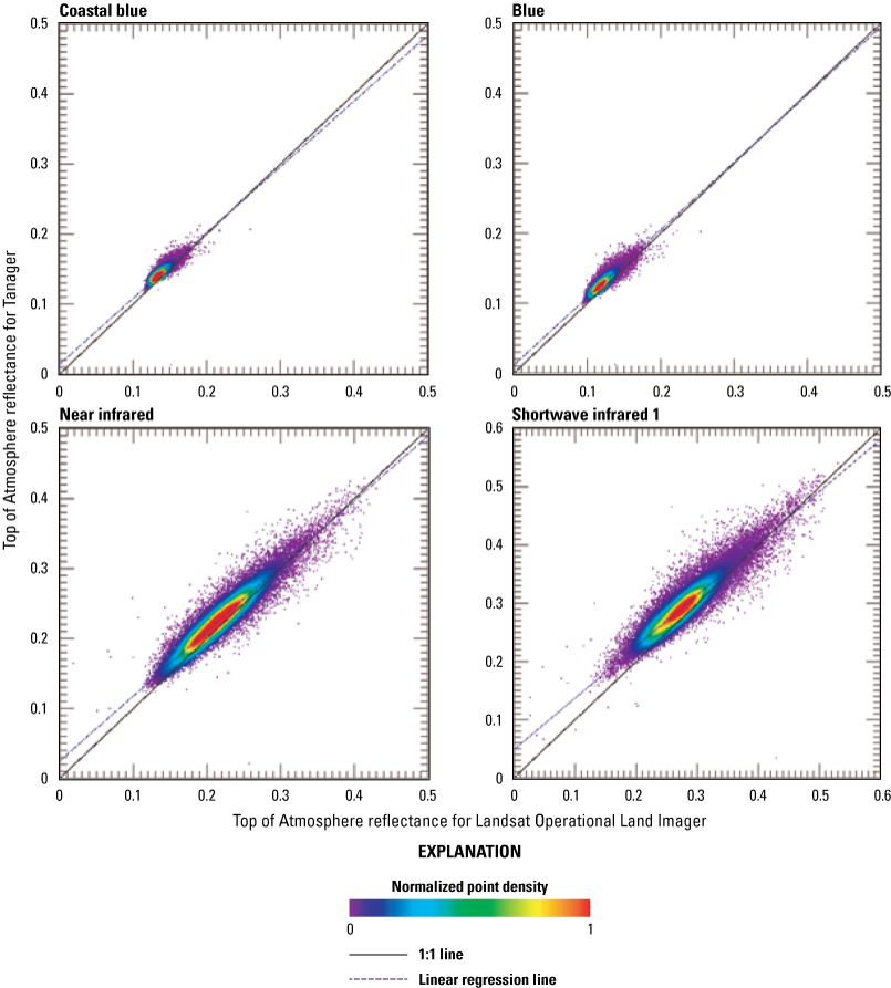
Radiometric scatterplots comparing Top of Atmosphere reflectance values derived from all seven bands of the spectrally resampled Australian Planet Labs PBC Tanager scene (20250305_010639_32_4001) and Landsat Operational Land Imager scene (LC09_L1TP_096076_20250305_20250305_02_T1).
Radiometric scatterplots comparing Top of Atmosphere reflectance values derived from all seven bands of the spectrally resampled Chinese Planet Labs PBC Tanager scene (20250523_055213_30_4001) and Landsat Operational Land Imager scene (LC08_L1TP_145028_20250523_20250602_02_T1).
Radiometric scatterplots comparing Top of Atmosphere reflectance values derived from all seven bands of the spectrally resampled Italian Planet Labs PBC Tanager scene (20250627_103759_58_4001) and Landsat Operational Land Imager scene (LC09_L1TP_190031_20250627_20250627_02_T1).
Comparison to Radiometric Calibration Network
The Tanager hyperspectral data were cross-checked against Radiometric Calibration Network (RadCalNet) data (https://www.radcalnet.org; RadCalNet, 2026).
The region of interest for the hyperspectral TOAR comparison was Railroad Valley, Nevada. The Tanager scenes used were collected on April 19, 2025 (20250419_190925_16_4001), and May 10, 2025 (20250510_191209_16_4001). The scenes were compared to the RadCalNet dataset RVUS_2025_109 and dataset RVUS_2025_130, respectively. The comparison plots for Tanager scenes and RadCalNet data are shown in figures 36 and 37.
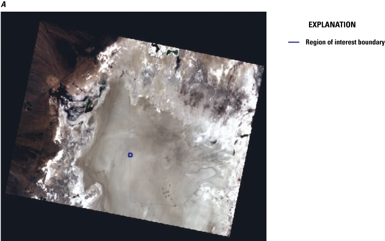
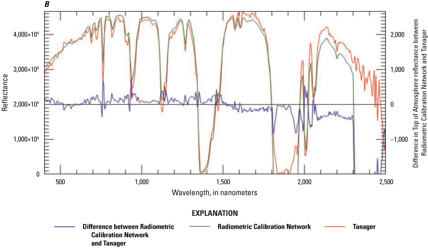
(A) Image of Railroad Valley, Nevada, Planet Labs PBC Tanager scene from April 19, 2025 (20250419_190925_16_4001), and (B) a graph comparing the Top of Atmosphere reflectance of the Tanager scene and the Radiometric Calibration Network dataset RVUS_2025_109. Image copyrighted by Planet Labs PBC, licensed under the Creative Commons Attribution-NonCommercial-ShareAlike 2.0 Generic license.
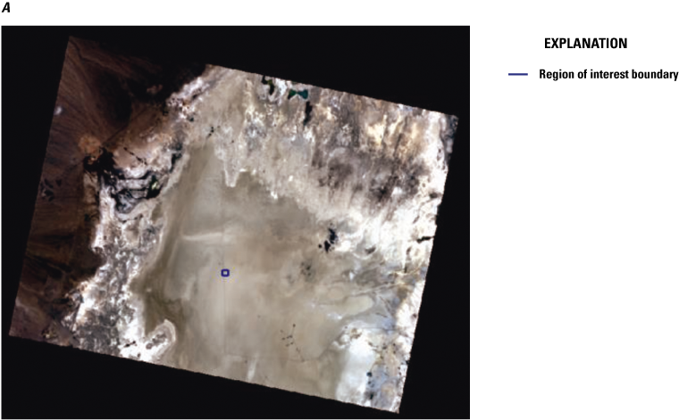
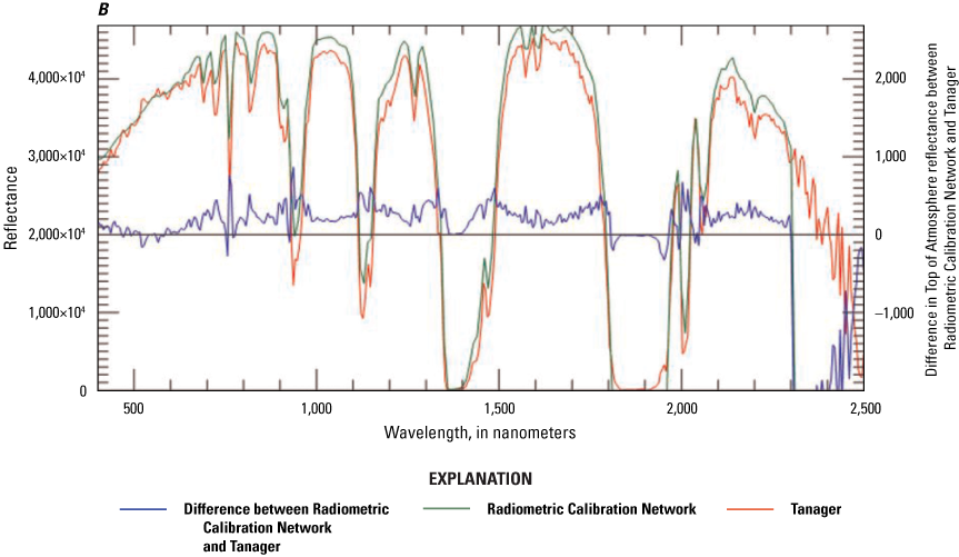
(A) Image of Railroad Valley, Nevada, Planet Labs PBC Tanager scene from May 10, 2025 (20250510_191209_16_4001), and (B) a graph showing comparing the Top of Atmosphere reflectance of the Tanager scene and the Radiometric Calibration Network dataset RVUS_2025_130. Image copyrighted by Planet Labs PBC, licensed under the Creative Commons Attribution-NonCommercial-ShareAlike 2.0 Generic license.
Spectral Shift
The sharp spectral absorption feature around the oxygen A-band near the 760-nm region provides a chance to evaluate spectral shift. The precisely known high resolution absorption of the sharp oxygen A-band region can be resampled using the spectral response function of Tanager. A look-up table around the oxygen A-band at several nominal Tanager hyperspectral bands is created by giving a range of spectral shifts. For a given Tanager scene and for all pixels along the sensor scanline, comparing the Tanager hyperspectral feature to the look-up table enables estimation of spectral shifts for all pixels. The May 10, 2025, Tanager scene over Railroad Valley is used for spectral shift analysis, and the results along the upper and lower scanlines are shown in figures 38 and 39, respectively.
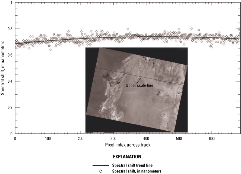
Plot showing the spectral shift analysis results derived from a Railroad Valley, Nevada, Planet Labs PBC Tanager scene (20250510_191209_16_4001) along the upper scanline. Image copyrighted by Planet Labs PBC, licensed under the Creative Commons Attribution-NonCommercial-ShareAlike 2.0 Generic license.
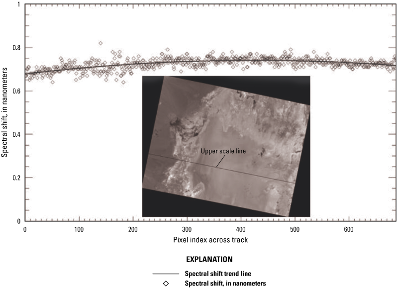
Plot showing the spectral shift analysis results derived from a Railroad Valley, Nevada, Planet Labs PBC Tanager scene (20250510_191209_16_4001) along the lower scanline. Image copyrighted by Planet Labs PBC, licensed under the Creative Commons Attribution-NonCommercial-ShareAlike 2.0 Generic license.
Spatial Performance
Because of the large GSD of the Tanager image, we used a spatial performance analysis technique that uses causeways. The Tanager image used for spatial analysis is 20250524_174343_30_4001. The linear feature in the image is the Lyndon B. Johnson Causeway in Aransas County, Texas (fig. 40).
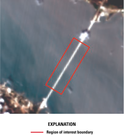
Image of Lyndon B. Johnson Causeway, Texas, Planet Labs PBC Tanager scene (20250524_174343_30_4001). The red box emphasizes a region of interest for spatial analysis on the Lyndon B. Johnson Causeway. Image copyrighted by Planet Labs PBC, licensed under the Creative Commons Attribution-NonCommercial-ShareAlike 2.0 Generic license.
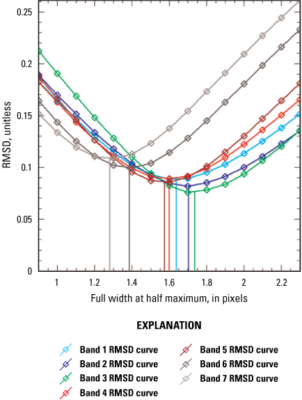
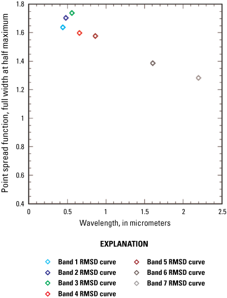
The geometric parameter for the bridge to generate an analog bridge model is 24.0 m wide, and the orientation angle of the bridge is about 58.66 degrees counterclockwise from east. The analog model is digitized based on the GSD of the image using the variable FWHMs. A simulated bridge image is compared to the sampled bridge image. Because the simulated bridge image is created much larger than the Tanager bridge image segment, the best matching segment out of the simulated image needs to be identified. A cross-correlation matrix is computed, and then the pixel shift that gives the maximum value of the cross-correlation matrix is identified. Once the pixel shift is identified and the matching simulated image segment is clipped, the root mean square difference (RMSD) values between the clipped portion of the simulated bridge with varying FWHMs and the bridge pixels sampled from the Tanager image are compared to find the FWHM associated with the minimum RMSD. The RMSD curve by varying FWHMs ranging from 0.7 to 1.9 pixels is shown in figure 41, and at the minimum position of the curve, an optimized FWHM value for the curve is determined. There are seven curves corresponding to each of the seven bands, and the result is shown in figure 41. All FWHMs determined from the minimum of the RMSD curves can be plotted as a function of wavelength, as shown in figure 42, and it shows the wavelength-dependent trend.
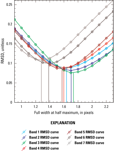
Graph of root mean square difference (RMSD) curves and corresponding minimum full width at half maximum lines for all bands derived from the Lyndon B. Johnson Causeway, Texas, Planet Labs PBC Tanager scene (20250524_174343_30_4001).
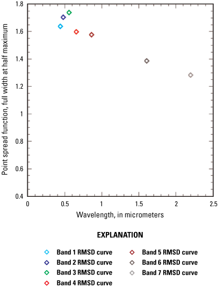
Graph of full width at half maximum for all bands derived from the Lyndon B. Johnson Causeway, Texas, Planet Labs PBC Tanager scene (20250524_174343_30_4001). [RMSD, root mean square difference]
Another Tanager image used for spatial analysis is 20250520_171558_31_4001. The linear feature in the image is the St. Louis Bay Bridge, Mississippi (fig. 43).
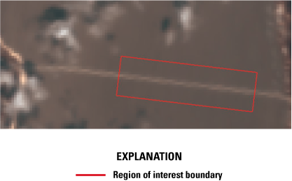
Image of St. Louis Bay Bridge, Mississippi, Planet Labs PBC Tanager scene (20250520_171558_31_4001). The red box emphasizes a region of interest for spatial analysis on the St. Louis Bay Bridge. Image copyrighted by Planet Labs PBC, licensed under the Creative Commons Attribution-NonCommercial-ShareAlike 2.0 Generic license.
The parameters to generate an analog bridge model are 30.0 m width and 7.07 degrees counterclockwise from east as an orientation angle of the bridge. In figure 44, the RMSD curve is shown by varying FWHMs ranging from 0.7 to 1.9 pixels, and at the minimum position of the curve, an optimized FWHM value for the curve is determined. Seven curves correspond to each of the seven bands, and the result is shown in figure 44. All FWHMs determined from the minimum of the RMSD curves can be plotted as a function of wavelength, as shown in figure 45, which shows the wavelength-dependent trend. Spatial performance analysis results are shown in table 7. Figure 46 illustrates how RER and MTF at Nyquist are estimated from FWHM; one specific FWHM result (1.28) from Lyndon B. Johnson Causeway was used as an example.
Root mean square difference (RMSD) curves and corresponding minimum full width at half maximum lines for all bands derived from the St. Louis Bay Bridge, Mississippi, Planet Labs PBC Tanager scene (20250520_171558_31_4001).
Full width at half maximum for all bands derived from the St. Louis Bay Bridge, Mississippi, Planet Labs PBC Tanager scene (20250520_171558_31_4001). [RMSD, root mean square difference]
Table 7.
Spatial performance of the Planet Labs PBC Tanager over the Lyndon B. Johnson Causeway, Texas, and the St. Louis Bay Bridge, Mississippi.[ID, identifier; RER, relative edge response; FWHM, full width at half maximum; MTF, modulation transfer function]
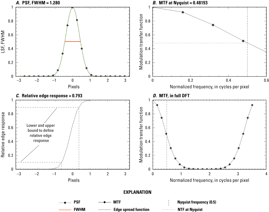
Graphs showing (A) point spread function with full width at half maximum in red line (upper left), (B) modulation transfer function with Nyquist frequency marked with a vertical dashed line, (C) relative edge response with lower and upper bound of the central one pixel marked with dashed lines (lower left), and (D) modulation transfer function in full range with Nyquist frequency marked with a vertical dashed line. [PSF, point spread function; FWHM, full width at half maximum; MTF, modulation transfer function; LSF, line spread function; DFT, discrete Fourier transform; one specific FWHM (1.28) from Lyndon B. Johnson Causeway was used to illustrate spatial analysis plots in this figure]
Summary and Conclusions
This report summarizes the sensor performance of the Planet Labs PBC Tanager satellite hyperspectral sensor based on the U.S. Geological Survey Earth Resources Observation and Science Cal/Val Center of Excellence (ECCOE) system characterization process. In summary, we have determined that Tanager has a band-to-band geometric performance in the range of −0.074 to 0.097 pixel, geometric performance relative to the Operational Land Imager in the range of −5.980 meters (−0.20 pixel) to 11.948 meters (0.40 pixel) offset in comparison to Landsat Operational Land Imager, offset of a radiometric comparison in the range of −0.004 to 0.056, slope of a radiometric comparison in the range of 0.830 to 1.066, and spectral shift in the range of 0.65 to 0.75 nanometer. The analysis of the point spread function gives the full width at half maximum in the range of 1.27 to 1.75 pixels, relative edge response in the range of 0.802 to 0.651, and the modulation transfer function at Nyquist in the range of 0.488 to 0.253.
In conclusion, the team has completed an ECCOE standardized system characterization of the Tanager hyperspectral sensor. Although the team followed characterization procedures that are standardized across the many sensors and sensing systems under evaluation, these procedures are customized to fit the individual sensor, as was done with Tanager. The team has acquired data, defined proper testing methodologies, carried out comparative tests against specific references, completed data analyses, and quantified sensor performance accordingly. The team also endeavored to retain all data, measurements, and methods. This is key to ensure that all data and measurements are archived and accessible and that the performance results are reproducible.
The ECCOE project and associated Joint Agency Commercial Imagery Evaluation partners are always interested in reviewing sensor and remote sensing application assessments and would like to review and discuss information on similar data and product assessments and reviews. If you would like to discuss system characterization with the U.S. Geological Survey ECCOE and (or) the Joint Agency Commercial Imagery Evaluation team, please email us at [email protected].
Selected References
Barsi, J.A., Lee, K., Kvaran, G., Markham, B. L., and Pedelty, J.A., 2014, The spectral response of the Landsat-8 Operational Land Imager: Remote Sensing, v. 6, no. 10, p. 10232–10251, accessed February 13, 2025, at https://doi.org/10.3390/rs61010232.
Cantrell, S.J., and Christopherson, J.B., 2024, Joint Agency Commercial Imagery Evaluation (JACIE) best practices for remote sensing system evaluation and reporting: U.S. Geological Survey Open-File Report 2024–1023, 26 p., accessed August 6, 2024, at https://doi.org/10.3133/ofr20241023.
Duren, R., Cusworth, D., Ayasse, A., Howell, K., Diamond, A., Scarpelli, T., Kim, J., O’neill, K., Lai-Norling, J., Thorpe, A., Zandbergen, S.R., Shaw, L., Keremedjiev, M., Guido, J., Giuliano, P., Goldstein, M., Nallapu, R., Barentsen, G., Thompson, D.R., Roth, K., Jensen, D., Eastwood, M., Reuland, F., Adams, T., Brandt, A., Kort, E.A., Mason, J., and Green, R.O., 2025, The Carbon Mapper emissions monitoring system: Atmospheric Measurement Techniques, v. 18, no. 22, p. 6933–6958. [Also available at https://doi.org/10.5194/amt-18-6933-2025.]
Keremedjiev, M.S., Roth, K.L., Barentsen, G., Haag, J., Bourne, H., Wurster, K., Radel, M., Mcdonald, T., Giuliano, P., Thompson, D.R., Guido, J., Duren, R., Green, R.O., and Seaman, K., 2025, Early results from the Tanager hyperspectral mission, in Algorithms, technologies, and applications for multispectral and hyperspectral imaging XXXI [Proceedings], Orlando, Fla., April 13–17, 2025: SPIE, v. 13455, accessed June 9, 2026, at https://doi.org/10.1117/12.3053498.
LeDuc, D., Roth, K.L., Barentsen, G., Annejohn, A., Wurster, K., Henze, C., Peters, E., Aati, S., Hernández Castilla, N., Gonzalez, A., Thompson, D.R., and Brodrick, P.G., 2026, Tanager L1B calibrated radiance algorithm theoretical basis (ver. 1.0): Planet Labs, PBC, 48 p., accessed June 9, 2026, at https://planet.widen.net/s/fpxrb5httq/planet-userdocumentation-tanagerl1b.
Planet Labs PBC, 2026, Tanager—Cutting-edge hyperspectral from orbit: Planet Labs PBC website, accessed March 5, 2026, at https://www.planet.com/constellations/tanager/.
RadCalNet, 2026, RadCalNet portal: Working Group on Calibration and Validation of the Committee on Earth Observation Satellites digital data, accessed March 5, 2026, at https://www.radcalnet.org.
U.S. Geological Survey, 2020, EROS CalVal Center of Excellence (ECCOE): U.S. Geological Survey website, accessed March 2021 at https://www.usgs.gov/core-science-systems/eros/calval.
U.S. Geological Survey, 2025, Landsat satellite missions: U.S. Geological Survey website, accessed February 13, 2025, at https://www.usgs.gov/landsat-missions/landsat-satellite-missions.
Zandbergen, S.R., Duren, R., Giuliano, P., Green, R.O., Haag, J.M., Moore, L.B., Shaw, L., and Mouroulis, P., 2022, Optical design of the Carbon Plume Mapper (CPM) imaging spectrometer, in Imaging spectrometry XXV—Applications, sensors, and processing [Proceedings], San Diego, Calif., August 21–26, 2022: SPIE, v. 12235, accessed June 9, 2026, at https://doi.org/10.1117/12.2633767.
Abbreviations
ECCOE
Earth Resources Observation and Science Cal/Val Center of Excellence
FWHM
full width at half maximum
GSD
ground sample distance
JACIE
Joint Agency Commercial Imagery Evaluation
OLI
Operational Land Imager
RadCalNet
Radiometric Calibration Network
RMSD
root mean square difference
TOAR
Top of Atmosphere reflectance
USGS
U.S. Geological Survey
For more information about this publication, contact:
Director, USGS Earth Resources Observation and Science Center
47914 252nd Street
Sioux Falls, SD 57198
605–594–6151
For additional information, visit: https://www.usgs.gov/centers/eros
Publishing support provided by the
USGS Science Publishing Network
Rolla and Baltimore Publishing Service Centers
Disclaimers
Any use of trade, firm, or product names is for descriptive purposes only and does not imply endorsement by the U.S. Government.
Although this information product, for the most part, is in the public domain, it also may contain copyrighted materials as noted in the text. Permission to reproduce copyrighted items must be secured from the copyright owner.
Suggested Citation
Kim, M., Park, S., Anderson, C., Clauson, J., Vrabel, J., and Sampath, A., 2026, System characterization report on Tanager (ver. 1.1, July 2026), chap. W of Ramaseri Chandra, S.N., ed., System characterization of Earth observation sensors: U.S. Geological Survey Open-File Report 2021–1030, 46 p., https://doi.org/10.3133/ofr20211030W.
ISSN: 2331-1258 (online)
| Publication type | Report |
|---|---|
| Publication Subtype | USGS Numbered Series |
| Title | System characterization report on Tanager |
| Series title | Open-File Report |
| Series number | 2021-1030 |
| Chapter | W |
| DOI | 10.3133/ofr20211030W |
| Edition | Version 1.0: May 18, 2026; Version 1.1: July 2, 2026 |
| Publication Date | May 18, 2026 |
| Year Published | 2026 |
| Language | English |
| Publisher | U.S. Geological Survey |
| Publisher location | Reston, VA |
| Contributing office(s) | Earth Resources Observation and Science (EROS) Center |
| Description | Report: vi; 46 p.; Dataset |
| Online Only (Y/N) | Y |
| Additional Online Files (Y/N) | Y |