

Compilation and Evaluation of Data Used to Identify Groundwater Sources Under the Direct Influence of Surface Water in Pennsylvania
Links
- Document: Report (7.61 MB pdf) , HTML , XML
- Data Release: USGS data release - Database used for the evaluation of data used to identify groundwater sources under the direct influence of surface water in Pennsylvania
- Version History: Version History (49.8 KB txt)
- NGMDB Index Page: National Geologic Map Database Index Page (html)
- Download citation as: RIS | Dublin Core
Acknowledgments
The authors would like to thank Pennsylvania Department of Environmental Protection, Bureau of Safe Drinking Water (PADEP, BSDW) hydrogeologic staff from the Southcentral, Northcentral, Southwest, and Southeast Regional Offices for providing public water-supply system source information from their respective regions. The authors also thank the staff of the PADEP, BSDW Central Office for providing partner courtesy reviews of this report.
Abstract
A study was conducted to compile and evaluate data used to identify groundwater sources that are under the direct influence of surface water (GUDI) in Pennsylvania. In the early 1990s, the Pennsylvania Department of Environmental Protection (PADEP) implemented the Surface Water Identification Protocol (SWIP) for the identification of GUDI sources. Since the establishment of the SWIP, PADEP has classified more than 500 individual sources across Pennsylvania as GUDI, but Pennsylvania’s complex geology and physiography provide a challenge for a uniform method of GUDI determination. Components used in this study to compile and evaluate data associated with GUDI determination include: (1) a preliminary review of file information for 43 public water-supply wells, (2) quality control and addition of data to PADEP’s database for public water-supply systems to prepare data for analysis, and (3) exploratory evaluation of existing GUDI sources in the database with respect to hydrogeologic and source-construction characteristics that are currently utilized in the assessment methodology.
Case files for 43 wells from PADEP’s Northcentral and Southcentral regions were reviewed to: (1) provide a better understanding of how the SWIP was applied in practice, (2) verify and compile missing data, and (3) find additional attributes not previously available that might explain a well’s categorization as GUDI. Review of file information showed that the SWIP outlined in PADEP technical guidance was usually followed, but for some sources, the GUDI determination was more complex and could not be easily summarized.
Data compiled for study analyses provided by PADEP include source data derived from public water-supply system case files, a source-information database for public water-supply systems, and Microscopic Particulate Analysis (MPA) results and associated water-quality data for public water-supply system groundwater sources. Data from the Pennsylvania Drinking Water Information System (PADWIS), which is PADEP’s database for public water-supply systems, were also used for this study. The PADWIS database originally included data for 12,147 groundwater sources (11,812 groundwater sources not under the direct influence of surface water (non-GUDI) wells and 335 GUDI wells). A subset (4,018 wells consisting of 3,842 non-GUDI wells and 175 GUDI wells) of the PADWIS database was created for an analysis and includes only community wells evaluated in accordance with the SWIP. MPA results for 631 community and noncommunity wells were compiled, along with associated water-quality data (alkalinity, chloride, Escherichia coli, fecal coliform, nitrate, pH, sodium, specific conductance, sulfate, total coliform, total dissolved solids, total residue, and turbidity) populated from the PADEP Bureau of Laboratories Sample Information System. Data compiled from sources other than PADEP include spatial data, both naturogenic (for example, average precipitation or distance to closest hydrologic feature) and anthropogenic (for example, percentage of developed or agricultural land cover within a specific vicinity of a public water-supply system well) data representing spatially derived variables.
Comparison among wells in the PADWIS dataset subset using the nonparametric Kruskal-Wallis test showed that GUDI wells had significantly older median construction years, shallower depths, and static water levels closer to the land surface than non-GUDI wells and that carbonate aquifers had the highest percentages of wells designated as GUDI (12 percent; 57 wells). Further comparison of wells in the PADWIS database subset using the Spearman’s rho monotonic correlation test illustrated that public water-supply wells designated as GUDI largely occur in unconfined aquifers and have high average yield and shallow static water levels. Assessment of the MPA database subset using the Kruskal-Wallis test showed wells with MPA total risk-factor scores that exceeded zero had older median construction years and shallower casing depths than wells with MPA total risk-factor scores of zero and that carbonate aquifers had the highest percentages of wells with MPA total risk-factor scores exceeding zero (30 percent; 63 wells). Spearman’s rho correlations showed that wells completed in aquifers with depths to major water-bearing zones closer to the land-surface had higher total risk-factor scores resulting from MPA samples.
Based on the results of the analyses described in this report, broad conclusions can be drawn regarding site-specific well characteristics as well as anthropogenic and naturogenic factors that could be responsible for a well being designated as GUDI, but the accuracy of these results is dependent on the quality of the data being analyzed. Ultimately, study results serve as an added resource for initial desktop screening of wells to determine if additional site-specific investigation is warranted and underscore the need for field evaluation.
Introduction
The Pennsylvania Department of Environmental Protection (PADEP) regulates public water-supply systems through implementation of the Pennsylvania Safe Drinking Water Act (SDWA) and associated Safe Drinking Water Regulations (25 Pa. Code 109) to assure that a safe and reliable supply of water is provided to consumers. Approximately 83 percent of the 12.8 million people residing in Pennsylvania obtain their drinking water from a public water-supply system (Pennsylvania Department of Environmental Protection, 2015). In addition to imposing adequate treatment techniques, PADEP uses a methodology to identify groundwater sources that are under the direct influence of surface water (GUDI) because surface water, and therefore GUDI sources, are prone to pathogenic contamination. Although hydrologists consider groundwater and surface water as a single resource (Winter and others, 1998), for the purposes of this report GUDI is defined as, “any water beneath the surface of the ground with the presence of insects or other macroorganisms, algae, organic debris or large diameter pathogens such as Cryptosporidium and Giardia lamblia, or significant and relatively rapid shifts in water characteristics such as turbidity, temperature, conductivity, or pH which closely correlate to climatological or surface-water conditions” (Pennsylvania Department of Environmental Protection, 2002a,b31). The term does not apply to finished water, which is defined as “water that is introduced into the distribution system of a public water-supply system and is intended for distribution and consumption without further treatment, except as necessary to maintain water quality in the distribution system” (Pennsylvania Department of Environmental Protection, 2002a, b31).
Groundwater sources that do not meet Pennsylvania’s regulatory definition for GUDI are considered groundwater sources not under the direct influence of surface water (non-GUDI) or groundwater, and these sources should not be as prone to pathogenic contamination. Cryptosporidium and Giardia lamblia are waterborne pathogenic protozoans that can reside in surface water or groundwater, and, if ingested by humans, they can cause the diarrheal diseases cryptosporidiosis and giardiasis, respectively. Contamination of drinking water with Cryptosporidium oocysts or Giardia lamblia cysts is of concern because they are both protected by an outer shell that makes them highly resistant to simple disinfection treatment techniques, such as chlorination, and capable of surviving several months in water without a host (Centers for Disease Control and Prevention, 2015).
Pennsylvania, in addition to other states, experienced numerous waterborne-disease outbreaks associated with public water-supply systems during the 1970s and 1980s (Pennsylvania Department of Environmental Protection, 2015). These outbreaks resulted in the U.S. Environmental Protection Agency (EPA) enacting the 1986 Amendment to the SDWA, also known as the Surface Water Treatment Rule (SWTR), which provided new regulations for filtering and disinfecting surface water and GUDI sources (U.S. Environmental Protection Agency, 1992). In 1989, Pennsylvania passed its own SWTR, which required all surface-water sources serving public water-supply systems to be filtered and disinfected and changed the definition of surface water to include “water directly influenced by surface water, which may include springs, infiltration galleries, cribs, or wells” (Pennsylvania Department of Environmental Protection, 2002a,b31). The EPA’s SWTR gave states with the authority to implement and enforce the SDWA within their jurisdictions the responsibility of identifying GUDI sources and required states to determine which community and non-community public water-supply systems were using GUDI sources by June 29, 1994, and June 19, 1999, respectively (U.S. Environmental Protection Agency, 1992; Pennsylvania Department of Environmental Protection, 2002b). In Pennsylvania, community systems are defined as public water-supply systems that provide water to the same population throughout the year, such as municipal systems, authorities, or mobile home parks, whereas non-community systems are public water-supply systems that can be nontransient or transient (Pennsylvania Department of Environmental Protection, 2015). Nontransient systems regularly serve at least 25 of the same people for at least 6 months a year (for example, schools, factories, or hospitals with their own water supplies), and transient systems serve transitory customers in nonresidential areas (for example, campgrounds, restaurants, or hotels with their own water supplies).
Because of the EPA’s SWTR, PADEP implemented the Surface Water Identification Protocol (SWIP) in the early 1990s to provide a methodology for the identification of GUDI sources (Pennsylvania Department of Environmental Protection, 2002b). More information about the SWIP and how PADEP identifies GUDI sources can be found in PADEP documentation (Pennsylvania Department of Environmental Protection, 2001; 2002a, b31; 2008). According to the Pennsylvania Drinking Water Information System (PADWIS; Pennsylvania Department of Environmental Protection, 2016), which is a database used by PADEP to inventory public water-supply systems, 560 individual public water-supply systems across Pennsylvania, of which 335 are public water-supply wells (table 1; fig. 1), have been classified as GUDI since the establishment of Pennsylvania’s SWIP. The U.S. Geological Survey (USGS) in cooperation with PADEP, has applied quality-control (QC) methods and analyzed a version of the PADWIS database, along with associated water-quality data provided by PADEP, to evaluate the associated data for identifying GUDI sources in Pennsylvania (Gross, 2022).
Table 1.
Available attributes in the Pennsylvania Drinking Water Information System (PADWIS) database for public water-supply systems identified as groundwater under the direct influence of surface water (GUDI) or groundwater not under the direct influence of surface water (non-GUDI).[Attribute availability is described in relation to the full PADWIS database (before the application of quality-control procedures) and the PADWIS database subset that is described later in the report. GUDI, groundwater source under the direct influence of surface water; non-GUDI, groundwater source not under the direct influence of surface water; PADEP, Pennsylvania Department of Environmental Protection; SWIP, surface water identification protocol; PVC, polyvinyl chloride]
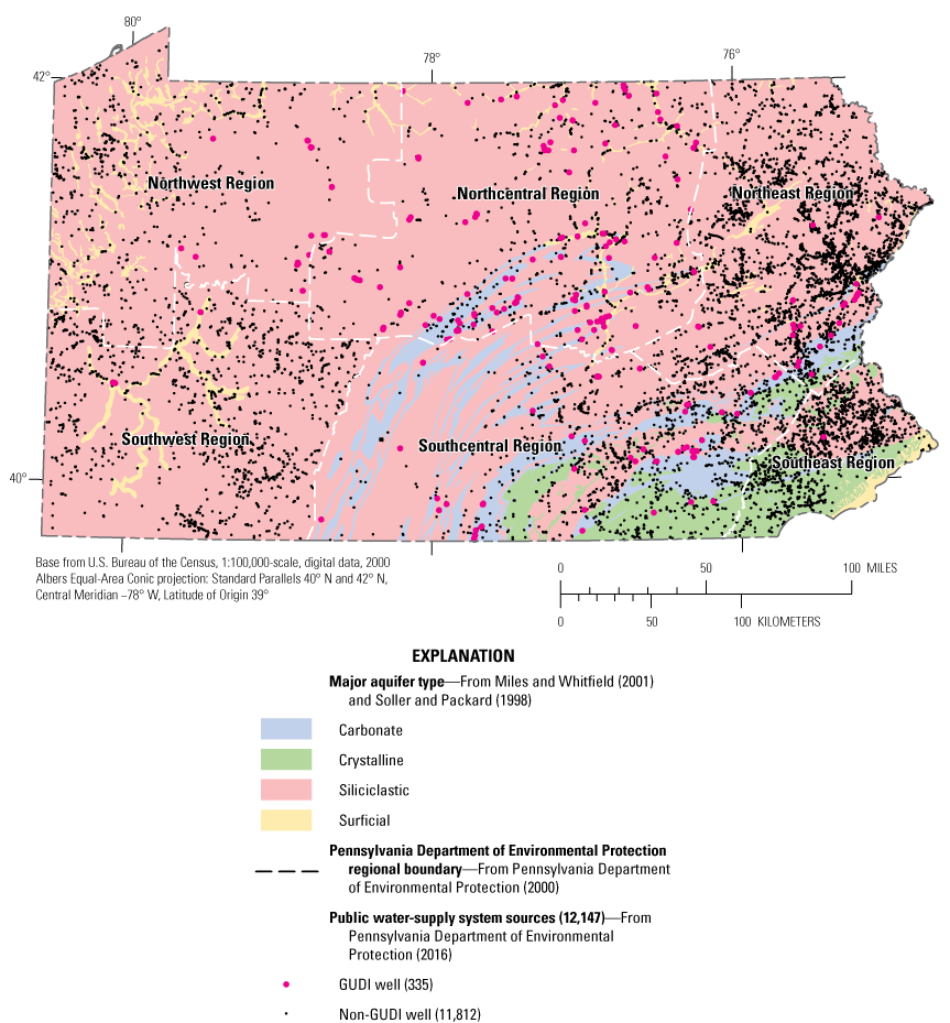
Map of public water-supply system wells classified as either groundwater source under the direct influence of surface water (GUDI) or non-GUDI, with Pennsylvania Department of Environmental Protection regions overlaid on major aquifer types.
Purpose and Scope
This report documents the following components of data compilation and evaluation: (1) a review of file information for 43 public water-supply system wells (hereafter referred to as wells) from the PADEP Northcentral and Southcentral regions to evaluate the SWIP and Microscopic Particulate Analysis (MPA) in GUDI determinations, (2) the addition of attributes to the PADWIS database including spatial anthropogenic (land cover and PADEP region) and naturogenic (geologic and physiographic, hydrologic, soil characterization, and topographic) data that could be potential indicators of GUDI designation or the presence of contaminants in MPA results, which was the impetus for the creation of three datasets (PADWIS database, PADWIS database subset, and MPA database subset) to be used for analysis (Gross, 2022), and (3) statistical summary and correlation analysis to evaluate existing GUDI sources in the databases with respect to hydrogeologic and source-construction characteristics that are currently utilized in the SWIP assessment methodology.
Review of Case Files for 43 Wells
Case files associated with 43 selected wells in the PADWIS database were reviewed to: (1) verify and compile missing data values for attributes in the PADWIS database and identify additional data not included in the PADWIS database that might help to explain a well’s susceptibility to surface-water influence, and (2) provide a better understanding of how the SWIP steps were applied in practice to generate data needed to evaluate wells. The distribution of GUDI wells across PADEP regions is uneven, with more than half (56 percent) located within the Northcentral region and just one in the Southeast region (fig. 2). The complex physical settings can be highly variable among wells across the state, and limited site-specific data make implementation of a uniform evaluation approach for GUDI difficult. This is likely a contributing factor explaining the uneven percentage of GUDI wells across the state (fig. 2). Source data derived from PADEP well case files included various types of documentation, such as hydrogeologic reports, PADEP-issued permits, GUDI determination decision letters, and monitoring plans—not all of which were available for each of the wells.
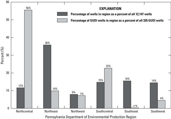
Percentage of public water-supply system wells and percentage of wells classified as groundwater sources under the direct influence of surface water (GUDI) within each Pennsylvania Department of Environmental Protection region.
Of the 43 case files reviewed, 30 were for wells located in the Southcentral region and 13 were for wells in the Northcentral region. These two regions were chosen for case file review because 79 percent of the GUDI wells in the PADWIS database were in these regions (fig. 2). In the Southcentral region, the case files of 30 wells that were considered susceptible to surface-water influence based on aquifer type and well characteristics were examined to gain a better understanding of the evidence used to determine why 19 of the wells were classified as GUDI and 11 were determined not to be GUDI. In the Northcentral region, case files were examined that had been classified as GUDI without undergoing 6 months of monitoring. (Pennsylvania Department of Environmental Protection, 2001, 2002b31).
Data Availability
Files associated with 43 wells in PADEP’s Northcentral and Southcentral regions were examined to verify and compile missing data values for PADWIS attributes that are important for conducting the SWIP. Although the PADWIS database includes most of the criteria used for the SWIP, such as major aquifer type, static water level, or whether the aquifer is confined (Pennsylvania Department of Environmental Protection, 2001, 2002b), it does not provide sufficient information to show what data were utilized to classify a well as GUDI. For example, the SWIP STATUS attribute (table 1) in the PADWIS database indicates if an evaluation was completed, but this attribute does not provide results for SWIP monitoring or the total risk-factor scores from any collected MPA samples, so it is not known which, if any, of the SWIP monitoring criteria or guidelines (Pennsylvania Department of Environmental Protection, 2001, 2002b) were utilized during the evaluation. As a result, some PADWIS attributes could have verification performed using information in the well files to change incorrect values to correct values or to fill in missing values. In addition, files were examined to find additional attributes that were not included in the PADWIS database that might help to explain a well’s susceptibility to surface-water influence.
In the Southcentral region, the well depth (DEPTH [FT] attribute, table 1) was found in the files for 18 selected wells. Six (33 percent) of the 18 values differed from the data values stored in the PADWIS database. Casing depth (CASING DEPTH [FT] attribute, table 1) was available for 15 wells. Three (20 percent) of the 15 values differed from the data values stored in the PADWIS database. Depth to water in the well (STATIC WATER LEVEL [FT] attribute, table 1) was found in the files associated with 14 (74 percent) of the 19 wells. According to PADEP’s SWIP, static water level in the well is a necessary attribute for determining if a source is susceptible to surface-water influence (Pennsylvania Department of Environmental Protection, 2001).
Other variables of importance to determine if additional monitoring and evaluation are needed on a source include the spatial coordinates that define a well’s location (LATITUDE and LONGITUDE attributes, table 1). Spatial coordinates for 11 wells in the Southcentral region were found in files associated with the wells, yet the spatial coordinates listed in the files for 9 (82 percent) of these 11 wells differed by 130 to 14,800 feet (ft) from the coordinates provided in the PADWIS database. Some of these discrepancies could be caused by assuming an incorrect datum, but most errors exceeded the error that would arise with a shift from North American Datum (NAD) 1927 to NAD 1983.
Files associated with wells also were evaluated to obtain specific data that were collected by completing the SWIP but unavailable as PADWIS attributes. For example, the distance (threshold distance of 200 ft) from a well to the nearest surface-water feature, such as a flowline, water feature, or water body, is not an attribute available for assessment in the PADWIS database (Pennsylvania Department of Environmental Protection, 2016), but this is an attribute that may require a well to be identified for further evaluation. Data describing the distance to the nearest surface-water feature were found in files for 9 (47 percent) of 19 selected wells examined in the Southcentral region. For most of the GUDI wells in the Southcentral region, the distance to the nearest surface-water feature was not evaluated as part of the initial screening because the static water level in the wells did not exceed 50 ft below the land surface. This highlights an important point when considering the primary threat of surface-water influence to a well. Instead of evaluating the relation between groundwater and surface water (for example, streams and lakes), the focus for these nine wells was water-quality variations and the potential for rapid infiltration of precipitation if preferential-flow pathways are available at or near the wellhead. Evaluation of this primary threat is fundamentally different compared to determining a hydraulic connection between an aquifer and stream or lake.
Pearson-correlation coefficients, which are derived from data (water-quality parameters, precipitation, and local surface-water conditions) collected by the water system during the 6-month SWIP monitoring program, that are considered high (> 0.40) can be used to classify a well as GUDI or to elicit MPA testing, but these results are not included in the PADWIS database. Pearson-correlation results from the SWIP monitoring were available in files for 14 (74 percent) of 19 selected wells designated as GUDI in the Southcentral region, whereas 9 (82 percent) of the 11 non-GUDI wells had Pearson-correlation results from the SWIP monitoring.
Results associated with MPA sample collection are an important, and often final, part of the evaluation process since these results are reported as the definitive presence or absence of specific bioindicators. MPA results were available in files associated with 15 (79 percent) of 19 selected wells in the Southcentral region, and 4 (44 percent) of the 9 non-GUDI wells with the SWIP monitoring results had associated MPA results.
Application of the Surface Water Identification Protocol
The SWIP consists of up to three steps: (1) screening for sources susceptible to surface-water influence based on aquifer type and well characteristics, (2) monitoring for six months to evaluate the Pearson-correlation results among water level, precipitation, or stream stage with selected water-quality parameters, and (3) sampling for particulates and organisms with an MPA. Overall, the best information from the well files about how the SWIP was followed and ultimately why a well was classified as non-GUDI or GUDI is contained in the letter of determination from PADEP to the water supplier. The letter summarizes the specific evidence from the evaluation that supports the determination. A letter of determination was available for 20 (47 percent) of the wells included in file reviews from selected PADEP regions.
File review of selected wells showed that for some sources the GUDI determination in practice is much more complex and cannot be easily summarized in a database such as PADWIS. One of the GUDI wells in the Southcentral region that illustrates this complexity was in service in 2013 as a community well classified as non-GUDI when the operator noticed an increase in turbidity and nitrate concentrations following precipitation events (Thomas Yeager, Pennsylvania Department of Environmental Protection, written commun., October 24, 2017). After notifying PADEP, the well was shut down, owing to elevated bacteria levels and the presence of bioindicators in water samples, and reclassified as GUDI in March 2013. Further investigation by the well owner revealed a cracked well casing that allowed surface water to drain into the well. The well was reconstructed, after which 6 months of SWIP monitoring was conducted and several MPA samples were collected by PADEP and the operator. The monitoring and MPA results showed a low risk for surface-water influence, so the well was classified as “groundwater” (non-GUDI) in December 2015. This process, which started with an astute water-system operator, took nearly two years to complete.
Review of the well files shows that application of a uniform evaluation approach for GUDI is difficult because of highly variable site-specific factors that need to be considered in applying the SWIP steps, but its effect is difficult to quantify. This is especially notable in the evaluation of results from the 6 months of SWIP monitoring because the Pearson-correlation results among the monitored parameters are commonly moderate (close to but not exceeding 0.40). In such cases, the results of analyses of the bacteria samples collected during the monitoring are sometimes used to provide additional rationale for requiring an MPA sample. The most ambiguous cases seem to be those with: (1) moderate Pearson-correlation results during the monitoring, (2) detections of some bacteria, and (3) a low-risk MPA sample with some organisms detected. In some of these cases, the presence of bacteria and other organisms was used as an indication of surface-water influence and as evidence to classify the source as GUDI; in other cases, despite the presence of bacteria, the source was not classified as GUDI given the low-risk MPA results in addition to the implementation of disinfection treatment practices.
Implementation of the SWIP in PADEP’s Southcentral and Northcentral regions is further summarized in the following sections based on the examination of well files. Files were examined to determine: (1) why 19 wells in the Southcentral region were classified as GUDI, (2) why 11 similar wells in the Southcentral region were determined to be groundwater (non-GUDI), and (3) why 13 wells in the Northcentral region were classified as GUDI without undergoing SWIP monitoring.
Examination of Case Files for 19 Wells Classified as Groundwater Under the Direct Influence of Surface Water in Southcentral Pennsylvania
Files for 19 Southcentral region wells classified as GUDI were reviewed. PADWIS included SWIP STATUS attributes for these wells, indicating that the steps of the protocol had been completed for the wells, but it was apparent from the file review that data from different steps were given different weighting. The files showed that all three steps of the SWIP were completed and documented for 15 (79 percent) of the 19 wells reviewed. Although it may have been available elsewhere, documentation fully explaining the reasoning behind classifying the other 4 wells (21 percent) as GUDI could not be found in the files associated with the wells. The rationale for classifying 15 of the wells as GUDI included:
-
• GUDI classification determined by all three SWIP steps.—For 12 (63 percent) of the 19 wells reviewed, the initial screening step showed the wells were highly susceptible to surface-water influence, six months of monitoring showed moderate Pearson-correlation results among water-quality parameters with bacteria present in samples, and the MPA results indicated moderate or high risk (total risk-factor score of 10 or greater). Data from the three SWIP steps supported classification of the wells as GUDI.
-
• GUDI classification determined by monitoring.—For 2 (11 percent) of the 19 files reviewed, the screening step showed that although the wells had a high susceptibility to surface-water influence, the MPA results indicated low risk (total risk-factor score lower than 10), so the GUDI determination was made on the basis of results from six months of monitoring that showed Pearson-correlation results between turbidity and precipitation greater than 0.4 with the presence of bacteria. Thus, data generated from two of the three SWIP steps supported classification of the wells as GUDI.
-
• GUDI classification determined by susceptibility and existing data from other wells in the same well field.—For 1 (5 percent) of the 19 wells reviewed, the screening step showed the well had a high susceptibility to surface-water influence, but there were no high Pearson-correlation results between water-quality parameters and precipitation during six months of monitoring, and the MPA result indicated low risk (total risk-factor score less than 10). The GUDI determination was made based on high bacteria counts found during six months of monitoring and because the well was similar in design and in the same aquifer setting as three other wells in the wellfield for which MPA results indicated high risk (total risk-factor score of 20 or greater). In this case, existing data from other wells in the same well field were used to classify the well as GUDI.
Examination of Case Files for 11 Wells Not Classified as Groundwater Under the Direct Influence of Surface Water in Southcentral Pennsylvania
Files for 11 wells in the Southcentral region for which the SWIP had been completed and which had been classified as groundwater (non-GUDI) sources were reviewed. The wells were drilled in carbonate rock and had water levels less than 100 feet [AQUIFER LITHOLOGY and STATIC WATER LEVEL(FT) attributes in PADWIS database, respectively; see table 1], indicating high susceptibility to surface-water contamination during the initial SWIP screening step, but none were classified as GUDI. The files were reviewed to determine: (1) how the SWIP steps were utilized, (2) to examine the data used to assign a source classification, and (3) to identify key factors that might be used to distinguish GUDI from non-GUDI wells prior to monitoring.
The review of files for the 11 non-GUDI wells in the Southcentral region showed more ambiguity in the determination than for the 19 GUDI wells. Because Pearson-correlation results between temperature, pH, turbidity, and specific conductance were usually less than 0.4, it appears that the presence of bacteria was used to help determine when an MPA sample was required for additional evidence. Though the 11 non-GUDI wells were flagged as sources susceptible to surface-water influence, monitoring was not required at 2 wells, and the collection of samples for MPA was not required at 6 wells. The rationale for classifying 15 of the wells as non-GUDI included:
-
• Non-GUDI classification determined by low-risk MPA result.—For 4 (36 percent) of the 11 wells reviewed, the initial screening step showed the wells were sources susceptible to surface-water influence, and six months of monitoring showed moderate Pearson-correlation results among water-quality parameters and high bacteria counts, so collection of an MPA sample was required. The non-GUDI classification appears to have been based heavily on an MPA result indicating low risk (total risk-factor score lower than 10).
-
• Non-GUDI classification determined by monitoring and low bacteria counts.—For 5 (46 percent) of the 11 wells reviewed, the screening step showed the wells were susceptible to surface-water influence, and 6 months of SWIP monitoring showed moderate Pearson-correlation results among water-quality parameters and low or no incidence of bacteria, so collection of MPA samples was not required. Low bacteria counts during the six months of SWIP monitoring appear to be the basis of the non-GUDI determination.
-
• Non-GUDI classification determined by other factors.—For 2 (18 percent) of the 11 wells reviewed, the screening step showed that these wells, completed in carbonate-rock aquifers with water levels less than 100 feet below land surface, were susceptible to surface-water influence, but the 6 months of monitoring was not required. After review of the files for these two wells, it was unclear why either six months of SWIP monitoring or the collection of MPA samples was not required. Since these wells were coded as being in the Wills Creek and Jacksonburg Formations, it is possible that they were determined to be in shale instead of carbonate-rock aquifers.
Examination of Case Files for 13 Wells Classified as Groundwater Under the Direct Influence of Surface Water in Northcentral Pennsylvania
Files associated with 13 GUDI wells in the Northcentral region were examined to understand why wells in this region had been classified as GUDI without requiring six months of SWIP monitoring. The PADWIS database indicates that 98 (29 percent) of 335 wells in Pennsylvania that were classified as GUDI were designated as such without receiving the six months of monitoring. Most of these 98 (85 percent) wells are in the Northcentral region (fig. 1). Although it may have been available elsewhere, documentation fully explaining the reasoning behind the classification of 2 (15 percent) of the 13 wells as GUDI could not be found in available files associated with the wells. Review of files in PADWIS for the wells for which such documentation was available provided the following insights regarding these wells being classified as GUDI:
-
• GUDI classification potentially determined by susceptibility.—For 6 (46 percent) of the 13 wells reviewed, the screening step showed the wells were sources susceptible to surface-water influence. Prior to conducting six months of monitoring, five of these wells were abandoned, the water-system operator began to filter the water from the sixth well prior to its dissemination, and all six wells were classified as GUDI in the PADWIS database. The six wells may indeed be GUDI, but further evidence beyond susceptibility for that determination is not available. Without any additional information, such as results from six months of monitoring or MPA sample collection, it is difficult to fully understand the conditions that would classify the well as GUDI.
-
• GUDI classification potentially determined by monitoring and susceptibility.— For 4 (21 percent) of the 13 wells for which files were reviewed, the classification of the wells as GUDI was not clearly documented in the available files associated with the wells. At two of these wells, six months of SWIP monitoring was completed, and the GUDI classification for these two wells seems to have been based on moderate Pearson-correlation results during the monitoring period. At the other two wells, the screening step indicated the wells were susceptible to surface-water influence, but the reason for classification of the wells as GUDI was not clearly documented in the files that were available for review.
-
• GUDI classification determined by susceptibility, high bacteria counts, and high-risk MPA result.—For 1 (8 percent) of the 13 wells reviewed, the screening step indicated that the well had high susceptibility to surface-water influence, bacteria were present at high levels in collected samples, and MPA results indicated high risk (total risk-factor score of 20 or greater). Even though six months of SWIP monitoring was not completed, bacteria and MPA samples were collected, and the associated results supported classification of the well as GUDI.
Compilation of Data
Information compiled for this study consists primarily of data provided by PADEP, including: (1) a source-information database for public water-supply systems called the Pennsylvania Drinking Water Information System (PADWIS; Pennsylvania Department of Environmental Protection, 2016), and (2) MPA results and associated water-quality data for public-water-supply systems. Additional data compiled from other sources include spatial data explanatory variables consisting of naturogenic data (for example, average precipitation or distance to closest hydrologic feature) and anthropogenic data (for example, percentage of developed or agricultural land cover within a specified distance of a well). Data were compiled in three separate databases, which were created based on data type and availability, and include:
-
• PADWIS database (12,147 wells),
-
• PADWIS database subset (4,018 wells), and
-
• MPA database subset (631 wells).
Pennsylvania Drinking Water Information System
The original version (before the application of quality-control (QC) procedures by the USGS) of the PADWIS database provided by PADEP for the purposes of this study contained information for 12,445 public water-supply sources, of which 560 sources were identified as GUDI and 11,885 sources as non-GUDI. For the non-GUDI sources, the database was modified by PADEP before being provided to USGS so that it only included public water-supply system source types of wells. Available attributes for GUDI and non-GUDI sources are listed in table 1 along with the number of wells that have available data for each attribute.
Pennsylvania Drinking Water Information System Database
Quality-control practices were applied to the PADWIS database, which involved checking spatial coordinates; verifying collection type information; excluding any sources not designated as wells; and verifying or removing data values that were either obvious errors or populated as zero rather than as “no data.” More detailed information about database QC can be found in Gross (2022). The database QC process resulted in a dataset containing 12,147 wells, consisting of 335 (3 percent) GUDI wells and 11,812 (97 percent) non-GUDI wells, hereafter referred to as the PADWIS database.
Most (around 63 percent) of the wells in the PADWIS database are non-community wells, 20 percent of which are designated as non-transient and 80 percent as transient. Community wells account for about 37 percent of the wells in the PADWIS database, and less than 1 percent of the total wells are designated as other system types, such as retail water facilities or bottled, bulk, or vended water. Most (90 percent) of the 335 wells classified as GUDI are community wells, whereas 64 percent of the 11,812 wells designated as non-GUDI are non-community wells.
According to the PADWIS database, the PADEP Northeast region contains the most wells (36 percent), the Northwest region contains the least (8 percent), and the other four regions have an intermediate number of wells (12 to 16 percent; fig. 2). The Northcentral region contains the highest percentage of GUDI wells, with 186 (13 percent) of the 1,410 wells in the region designated as GUDI. Of the total 335 wells in the PADWIS database classified as GUDI, 56 percent are in the Northcentral region, and 76 wells (23 percent) are in the Southcentral region (fig. 2). The Southeast region has only one GUDI well.
The SWIP status attribute in the PADWIS database (Pennsylvania Department of Environmental Protection, 2016) indicates 98 (approximately 29 percent) of the 335 GUDI wells were designated GUDI where SWIP monitoring was not required. Most of these wells are in the Northcentral region (fig. 3). Of the 98 wells without SWIP monitoring requirements, 78 (80 percent) had a SWIP finalization date between 1991 and 2000, indicating the classification of wells as GUDI without required SWIP monitoring occurred prior to 2001. In addition, the PADEP’s Guidance for Surface Water Identification Protocol (Pennsylvania Department of Environmental Protection, 2001) indicates that MPA testing may be conducted for susceptible sources prior to the SWIP monitoring; thus, an initial MPA sample may have indicated a moderate or high risk of susceptibility to surface-water influence.
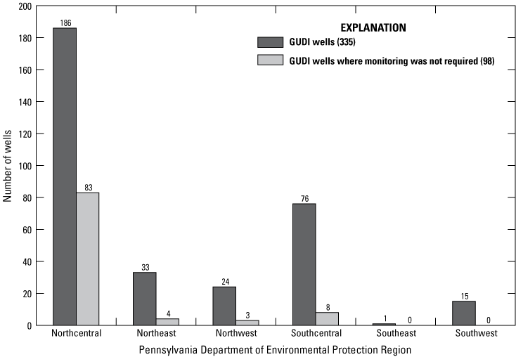
Number of public water-supply system wells classified as groundwater sources under the direct influence of surface water (GUDI) and number of wells classified as GUDI without the receiving the six months of monitoring, by Pennsylvania Department of Environmental Protection region.
The SWIP STATUS attribute in the PADWIS database also indicates “Not Evaluated–Filtered” for 121 wells, of which 108 were classified as GUDI and 13 classified as non-GUDI. These 121 wells essentially bypassed the SWIP because adequate treatment techniques were either already in place or were being installed in compliance with the SWTR. Of the 121 wells meeting these criteria, most were in the Northcentral (39 wells; 32 percent) and Southcentral (34 wells; 28 percent) regions, likely because these two regions have the highest number of GUDI wells statewide.
Pennsylvania Drinking Water Information System Database Subset
A subset of the PADWIS database was extracted to include only community wells that were indicated in the database to have undergone the SWIP to determine a source classification of GUDI or non-GUDI; this was an effort to only include sources in the study analysis that had been through a comparable evaluation process to receive GUDI or non-GUDI classification (Pennsylvania Department of Environmental Protection, 2010). Therefore, sources indicated in the PADWIS database with the SWIP STATUS attributes of “Completed—Monitoring Not Required” or “Completed—Source Monitored,” were included in this database subset.
This subset of the PADWIS database contains information for 4,018 community wells with 176 wells identified as GUDI and 3,842 sources identified as non-GUDI, hereafter referred to as the PADWIS database subset, with GUDI wells clustered in the north-central and central parts of the State (fig. 4). In addition to the spatial distribution of the PADWIS database subset, figure 4 also shows the statewide spatial distribution of this subset in relation to major aquifer type and physiographic provinces, which will be discussed in greater detail. The regional distribution of the 176 GUDI wells in this data subset includes a majority of GUDI wells in the Northcentral (140 [80 percent] of 176) and Southcentral (21 [12 percent] of 176) regions and the remaining four regions containing between 1 and 9 GUDI wells.
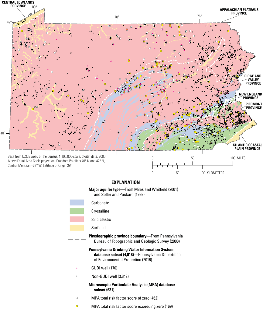
Map showing the spatial distribution of the Pennsylvania Drinking Water Information System Database subset and the Microscopic Particulate Analysis database subset in relation to major aquifer types and physiographic provinces in Pennsylvania.
Microscopic Particulate Analysis Database Subset
MPA sample results were obtained from the PADEP Bureau of Laboratories (BOL) files, and associated water-quality data were obtained from the PADEP BOL, Sample Information System. All groundwater samples that generated analytical laboratory results and included in this study were collected by PADEP staff and analyzed by BOL.
A digital database of 2,327 MPA results for samples collected from public water-supply systems between 1990 and 2014 was provided by PADEP. This database included analytical MPA results determined from methods in US Environmental Protection Agency (1992), including bioindicator counts and associated risk-factor scores for groundwater samples. All samples were collected and analyzed after the introduction of the SWIP in the early 1990s. Each MPA sample result was stored with a unique sample identification value and binary variables specifying absence or presence of primary bioindicators. The digital database of MPA results did not contain numeric values for the actual counts of individual bioindicators.
In addition, PADEP provided 1,979 individual MPA digital result sheets containing a sample number, date, and numeric information on the actual counts of primary bioindicators per 100 gallons. These sheets contained assigned risk-factor scores for each bioindicator based on those counts. A database of the digital result sheets was created to store the provided results, and this database was manually related to the original MPA database using unique sample identification values. In each database, records with the same sample number, collection date, and results were assumed to be duplicates, and only one record was retained. Conversely, records with the same sample number but different collection dates, collection times, and results were differentiated by “A” and “B” qualifiers added to the end of these sample numbers. This process yielded a total of 1,749 samples that were able to be matched between the two MPA databases to create a combined MPA database containing both the absence or presence indicator data and the numeric values for bioindicator counts.
Various amounts of records for public water-supply systems in the combined MPA database were stored with three of the source’s attributes—PWSID, SYSTEM NAME, and (or) SOURCE ID; see table 1 for attribute definitions—from the PADWIS database to indicate the source being tested. These three attributes were not always exact matches between the combined MPA and PADWIS databases and contained inconsistencies in naming associated with water system name changes, consolidation of sources following the completion of the MPA, or general transcription errors. Therefore, sources from the combined MPA database were manually matched with associated PADWIS database records based on whichever of these three attributes were available for each source. A total of 835 MPA results for 699 public water-supply systems from the combined MPA database were able to be joined with their respective source record in the PADWIS database. Of the 699 public water-supply systems, 631 had COLLECTION TYPE attributes of “Well,” while two sources had COLLECTION TYPE attributes of “Other,” and 66 were designated as “Spring.” Only the 631 sources with COLLECTION TYPE attributes coded as “Well” in the PADWIS database were included from the combined dataset of MPA results to be used for statistical analysis because the site-specific conditions causing a well to have a high MPA result are expected to be different than, and not necessarily representative of, site-specific conditions for sources like infiltration galleries, Ranney wells, cribs, and springs (Pennsylvania Department of Environmental Protection, 2002b). These 631 wells, which were associated with 749 MPA results, resulted in a dataset with 84 GUDI wells (a total of 117 results with the number of results per source ranging from 1 to 4) and 547 non-GUDI wells (a total of 632 results with number of results per source ranging from 1 to 4).
Water-quality samples are typically collected from wells concurrently with the MPA sample and analyzed by the BOL. Water-quality parameters or constituents tested for and associated with the MPAs typically include some combination of the following list of parameters:
-
• alkalinity in milligrams per liter (mg/L),
-
• chloride in mg/L,
-
• Escherichia coli (E. coli) in colony-forming units per 100 milliliters (CFU/100 mL),
-
• fecal coliform in CFU/100 mL,
-
• nitrate in mg/L,
-
• pH in standard units,
-
• sodium in mg/L,
-
• specific conductance in micromhos per centimeter at 25 degrees Celsius (°C),
-
• sulfate in mg/L,
-
• total coliform in CFU/100 mL,
-
• total dissolved solids in mg/L dried at 105°C,
-
• total residue in total solids dried at 103–105°C, and
-
• turbidity in Nephelometric Turbidity Units.
PADEP was able to compile and provide results for all or some of the previously listed water-quality parameters for the 749 MPA results that were matched with the PADWIS database. Results of analyses for these water-quality parameters were compiled from the BOL Sample Information System database that houses laboratory results for samples collected by PADEP’s Safe Drinking Water Program staff, including results for groundwater samples collected concurrently with the MPA sample. For 95 wells that were sampled more than once, the MPA and water-quality results from the most recent sampling event were retained for statistical analysis for this study, which resulted in the removal of 118 samples. Therefore, the MPA data analyses included in this study account for the most recent MPA collected from the well, regardless of the season in which it was collected.
The MPA dataset used for analysis consisted of MPA and water-quality results for 631 wells (84 GUDI, 547 non-GUDI), hereafter referred to as the MPA database subset, with results for water-quality parameters (see previous list) populated for 49 to 417 wells. Of the 631 wells included in the MPA database subset, 419 (66 percent) are community wells, and 212 (34 percent) are considered non-community (transient and non-transient) and other use types (bottled water and retail water facility).
For the MPA database subset of 631 wells, 169 (27 percent) had an MPA total risk-factor score exceeding zero (fig. 4), and 53 (8 percent) had a moderate (a score between 10 and 19) or high (a score of 20 or greater) risk MPA result classification (fig. 5). MPAs associated with the MPA database subset were collected between 1996 and 2014. The years with the highest amounts of MPAs collected were between 2003 and 2007 (292 [46 percent] of 631 MPAs) and are highlighted in figure 5. Years 2003–06 had the highest amount of MPAs with total risk-factor scores exceeding zero (82 [49 percent] of 169 MPAs) and 2006 had the highest number of moderate or high-risk MPA result classifications (10 [19 percent] of 53 MPAs) (fig. 5). Most of the MPAs were completed in the month of April (100 [16 percent] of 631 MPAs) and were also generally collected from April through July (319 [51 percent] of 631 MPAs), which were also the months with the highest number of MPA total risk-factor scores exceeding zero (94 [56 percent] of 169 MPAs) (fig. 6).
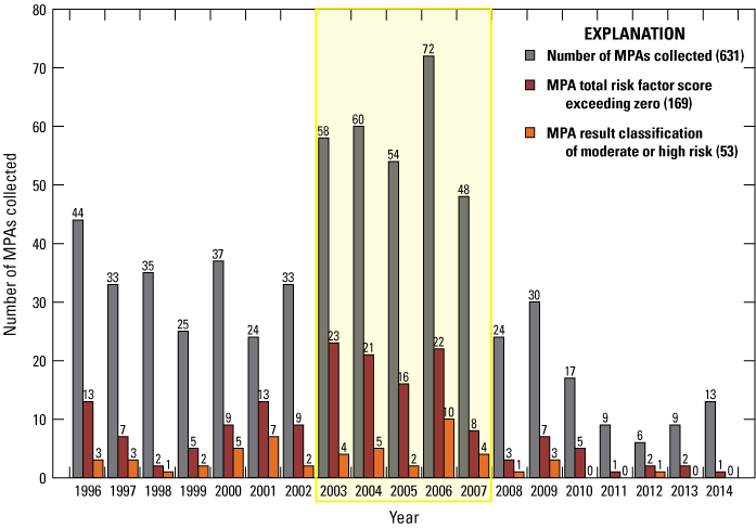
Number of Microscopic Particulate Analyses (MPAs) collected by year with number of MPAs with total risk-factor scores exceeding zero and number of moderate or high-risk MPAs. Years with the highest amounts of MPAs collected (2003–07) are highlighted with a yellow box. Numbers in parentheses and above bars are total number of wells.
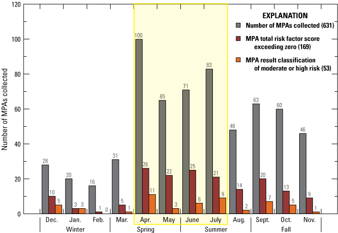
Number of Microscopic Particulate Analyses (MPAs) collected by month with seasons indicated and number of MPAs with total risk-factor scores exceeding zero and number of moderate or high-risk MPAs. Months with the highest amounts of MPAs collected (April, May, June, and July) are highlighted with a yellow box. Numbers in parentheses and above bars are total number of wells.
The regional distribution of the 631 wells with associated MPAs is like that of the total amount of GUDI wells, with the Northcentral and Southcentral regions having the highest number of wells with MPAs (fig. 7). Unlike the geographic distribution of total GUDI wells, the Southeast region had just one GUDI well (fig. 3). The Southeast region had 89 (14 percent) of 631 wells with MPAs, with 26 (29 percent) of the 89 MPAs exceeding zero and only 2 (2 percent) of the 89 MPAs classified as moderate or high risk (fig. 7). The Northcentral region, which had the highest number of total GUDI wells (186 [56 percent] of 335), also had the highest number of wells with MPAs (276 [44 percent] of 631). In the Northcentral region, 58 (21 percent) of 276 MPAs exceeded 0, and 22 (8 percent) of 276 MPAs were classified as moderate or high risk (fig. 7).
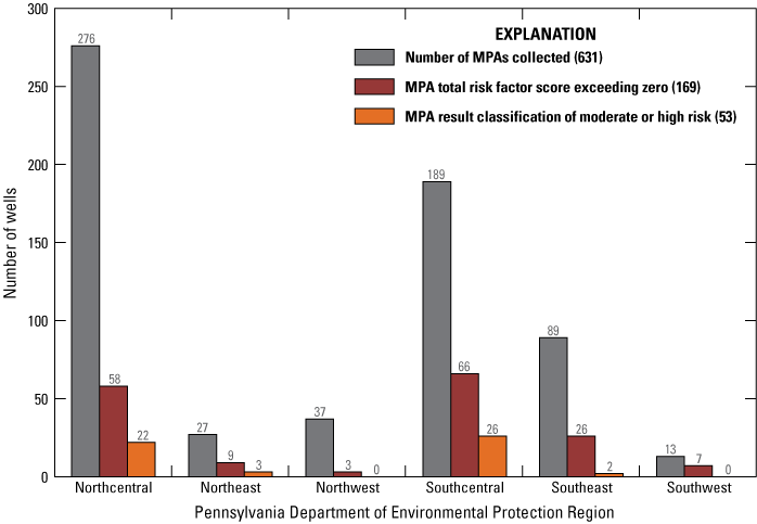
Number of public water-supply system wells with Microscopic Particulate Analysis (MPA) results, number of wells with MPA total risk-factor score exceeding zero, and number of wells with a moderate or high-risk MPA result classification, by Pennsylvania Department of Environmental Protection region.
Spatial Data
Spatial data consist of numeric and binary variables, representing anthropogenic (land cover and PADEP region) and naturogenic (geologic and physiographic, hydrologic, soil characterization, and topographic) data, which were compiled and extracted for the 12,147 wells in the PADWIS database. These data add attributes to the database that are potential indicators of the influence of surface water on water in the wells (table 2). Numeric (continuous) variables represent conditions at the spatial coordinates associated with the well (for example, percentage of developed land cover within a specific radius of the well, or percentage of clay content in the soil at the well), whereas binary variables indicate whether a well is within or outside of a mapped feature (for example, in a carbonate major aquifer type in the Piedmont physiographic province). Spatial data included only those mapped features that could be represented in a geographic information system (GIS); the mapped features ranged in scale from 1:24,000 to 1:250,000.
Table 2.
Summary of anthropogenic and naturogenic explanatory variable spatial data that were compiled and extracted for wells in the Pennsylvania Drinking Water Information System database. These data contribute additional attributes in the database that are potential indicators of groundwater under the direct influence of surface water or the presence of bioindicators in Microscopic Particulate Analysis results.[GIS, geographic information system]
| Explanatory variable | Description | Data source(s) | Original data GIS format | Original data resolution | Variable type |
|---|---|---|---|---|---|
| AG200 | Average area of agricultural land cover within a 200-foot (61-meter) radius (in percent) | U.S. Geological Survey (2014b) | Raster | 1:24,000 | Numeric |
| AG1640 | Average area of agricultural land cover within a 1,640-foot (500-meter) radius (in percent) | U.S. Geological Survey (2014b) | Raster | 1:24,000 | Numeric |
| DEV200 | Average area of developed land cover within a 200-foot (61-meter) radius (in percent) | U.S. Geological Survey (2014b) | Raster | 1:24,000 | Numeric |
| DEV1640 | Average area of developed land cover within a 1,640-foot (500-meter) radius (in percent) | U.S. Geological Survey (2014b) | Raster | 1:24,000 | Numeric |
| NC | Northcentral region (1 = in region, 0 = all other) | Pennsylvania Department of Environmental Protection (2000) | Raster | 1:24,000 | Binary |
| NE | Northeast region (1 = in region, 0 = all other) | Pennsylvania Department of Environmental Protection (2000) | Raster | 1:24,000 | Binary |
| NW | Northwest region (1 = in region, 0 = all other) | Pennsylvania Department of Environmental Protection (2000) | Raster | 1:24,000 | Binary |
| SC | Southcentral region (1 = in region, 0 = all other) | Pennsylvania Department of Environmental Protection (2000) | Raster | 1:24,000 | Binary |
| SE | Southeast region (1 = in region, 0 = all other) | Pennsylvania Department of Environmental Protection (2000) | Raster | 1:24,000 | Binary |
| SW | Southwest region (1 = in region, 0 = all other) | Pennsylvania Department of Environmental Protection (2000) | Raster | 1:24,000 | Binary |
| CARB | Carbonate major aquifer type (1 = carbonate, 0 = all other) | Miles and Whitfield (2001) and Soller and Packard (1998) | Polygon | 1:250,000 | Binary |
| CRYST | Crystalline major aquifer type (1 = crystalline, 0 = all other) | Miles and Whitfield (2001) and Soller and Packard (1998) | Polygon | 1:250,000 | Binary |
| SIL | Siliciclastic major aquifer type (1 = siliciclastic, 0 = all other) | Miles and Whitfield (2001) and Soller and Packard (1998) | Polygon | 1:250,000 | Binary |
| SURF | Surficial major aquifer type (1 = surficial, 0 = all other) | Soller and Packard (1998); Pennsylvania Bureau of Topographic and Geologic Survey (2008) | Polygon | 1:250,000 | Binary |
| APP | Appalachian Plateaus physiographic province (1 = Appalachian Plateaus, 0 = all other) | Pennsylvania Bureau of Topographic and Geologic Survey (2008) | Polygon | 1:250,000 | Binary |
| NE | New England physiographic province (1 = New England, 0 = all other) | Pennsylvania Bureau of Topographic and Geologic Survey (2008) | Polygon | 1:250,000 | Binary |
| PCARB | Carbonate major aquifer types in the Piedmont physiographic province (1 = Piedmont, 0 = all other) | Pennsylvania Bureau of Topographic and Geologic Survey (2008) | Polygon | 1:250,000 | Binary |
| PCRYST | Crystalline major aquifer types in the Piedmont physiographic province (1 = Piedmont, 0 = all other) | Pennsylvania Bureau of Topographic and Geologic Survey (2008) | Polygon | 1:250,000 | Binary |
| PSIL | Siliciclastic major aquifer types in the Piedmont physiographic province (1 = Piedmont, 0 = all other) | Pennsylvania Bureau of Topographic and Geologic Survey (2008) | Polygon | 1:250,000 | Binary |
| RVCARB | Carbonate major aquifer types in the Ridge and Valley physiographic province (1 = Ridge and Valley, 0 = all other) | Pennsylvania Bureau of Topographic and Geologic Survey (2008) | Polygon | 1:250,000 | Binary |
| RVCRYST | Crystalline major aquifer types in the Ridge and Valley physiographic province (1 = Ridge and Valley, 0 = all other) | Pennsylvania Bureau of Topographic and Geologic Survey (2008) | Polygon | 1:250,000 | Binary |
| RVSIL | Siliciclastic major aquifer types in the Ridge and Valley physiographic province (1 = Ridge and Valley, 0 = all other) | Pennsylvania Bureau of Topographic and Geologic Survey (2008) | Polygon | 1:250,000 | Binary |
| NHDFT | Distance in feet to nearest National Hydrography Dataset feature (flowline, water feature, water body) | U.S. Geological Survey (2014a) | Polygon, line | 1:100,000 | Numeric |
| NHD200 | NHDFT variable coded as a binary variable (1 = less than or equal to 200 feet, 0 = greater than 200 feet) | U.S. Geological Survey (2014a) | Polygon, line | 1:100,000 | Binary |
| PRE | Average precipitation from 1971 to 2000 (in inches per year) | PRISM Climate Group at Oregon State University (2006) | Raster | 1:250,000 | Numeric |
| RECH | Average groundwater recharge from 1951 to 1980 (in millimeters per year) | Wolock (2003) | Raster | 1:250,000 | Numeric |
| AWCAVE | Average soil available water capacity (in percent) | Wolock (1997) | Raster | 1:250,000 | Numeric |
| CLAYAVE | Average soil clay content (in percent) | Wolock (1997) | Raster | 1:250,000 | Numeric |
| PERMAVE | Average soil permeability (in centimeters per hour) | Wolock (1997) | Raster | 1:250,000 | Numeric |
| ROCKDEPAVE | Average soil thickness (in centimeters) | Wolock (1997) | Raster | 1:250,000 | Numeric |
| SANDAVE | Average soil sand content (in percent) | Wolock (1997) | Raster | 1:250,000 | Numeric |
| SILTAVE | Average soil silt content (in percent) | Wolock (1997) | Raster | 1:250,000 | Numeric |
| SLOPEAVE | Average soil land-surface slope (in percent) | Wolock (1997) | Raster | 1:250,000 | Numeric |
| ELEV | Land-surface elevation above sea level (in meters, North American Vertical Datum of 1988) | U.S. Geological Survey (2009) | Raster | 1:24,000 | Numeric |
| KARST | Distance to nearest karst feature, including sinkholes, surface depressions, surface mines, and caves (in feet) | Pennsylvania Bureau of Topographic and Geologic Survey (2007) | Point | 1:24,000 | Numeric |
| KARST200 | KARST variable coded as a binary variable (1 = less than or equal to 200 feet, 0 = less than 200 feet) | Pennsylvania Bureau of Topographic and Geologic Survey (2007) | Point | 1:24,000 | Numeric |
| TPI | Topographic position index classification (1 = Valleys, 2 = Lower Slopes, 3 = Gentle Slopes, 4 = Steep Slopes, 5 = Upper Slopes, 6 = Ridges) | U.S. Geological Survey (2009) | Raster | 1:24,000 | Numeric |
Anthropogenic Data
Land-cover data assessed included 30-meter resolution agricultural and developed land-cover classifications from the 2011 National Land Cover Database (NLCD) (U.S. Geological Survey, 2014b). The Hay/Pasture and Cultivated Crops classifications from the 2011 NLCD were grouped to create the agricultural land-cover classification used for this study to represent a possible source of animal fecal matter in groundwater from cattle or manure (Olson and others, 2004). The Open Space, Low Intensity, and Medium Intensity classifications from the 2011 NLCD were grouped to create the developed land-cover classification used for this study to represent rural, developed areas that are more likely to be using septic systems that are a possible source of contamination (Nnadi and Fulkerson, 2002; Craun and others, 1998). Average percentages of agricultural and developed land cover within a 200-foot (61-meter) radius of the well and a 1,640-foot (500-meter) radius of the well were calculated. A 200-foot (61-meter) radius is the surface-water setback distance utilized by the PADEP for initial screenings of groundwater sources. (Pennsylvania Department of Environmental Protection, 2002b). A 1,640-foot (500-meter) radius has been used in other studies and was statistically significant in reported models (Ayotte and others, 2012; Lindsey and others, 2006; Lindsey and others, 2009). These radii are not necessarily assumed to be actual contributing areas to the well, but data compiled for these areas are representative of land-surface characteristics near the wellhead.
Geographical divisions representing six PADEP office regions were also considered for analysis to see if variations in data availability and GUDI designations exist across the regions (fig. 1; Pennsylvania Department of Environmental Protection, 2000). PADEP regional offices directly implement the Safe Drinking Water Program in Pennsylvania. Each regional field office is meant to be structured in the same manner to consistently implement programs and services statewide (Pennsylvania Department of Environmental Protection, 2018). The six PADEP office regions include the Northeast, Northcentral, Northwest, Southeast, Southcentral, and Southwest regions (fig. 1). Although the PADWIS database included regional locations for each well (REGION attribute; table 1), spatial data (from Pennsylvania Department of Environmental Protection, 2018) were used to verify and independently define the region where each well was spatially located. Differences between PADWIS and spatial regional location data are listed in table 3. According to the PADWIS database REGION attribute (table 1; Pennsylvania Department of Environmental Protection, 2016) and data extracted for wells from regional spatial data (from Pennsylvania Department of Environmental Protection, 2000), a total of 47 wells (less than 1 percent of 12,147 wells) had spatial locations that did not match the regional location listed in the PADWIS database.
Table 3.
Regional location differences between the Pennsylvania Drinking Water Information System (PADWIS) database and spatial data.Naturogenic Data
Geologic data include major aquifer types (Miles and Whitfield, 2001; Soller and Packard, 1998) and physiographic provinces (Pennsylvania Bureau of Topographic and Geologic Survey, 2008) in Pennsylvania (fig. 4) used to characterize GUDI well occurrence or presence of bioindicators in MPA results in specific bedrock types and geographic areas. Pennsylvania falls partly within six physiographic provinces, including the Appalachian Plateaus, Atlantic Coastal Plain, Central Lowlands, New England, Piedmont, and Ridge and Valley Provinces, and contains a complex geology, with 193 geologic units recognized by the Pennsylvania Bureau of Topographic and Geologic Survey (Pennsylvania Bureau of Topographic and Geologic Survey, 2008; Miles and Whitfield, 2001). Additionally, geologic units across the northern part of the State are overlain by unconsolidated sand and gravel glacial deposits (Soller and Packard, 1998). The State’s complex geology and physiography poses a challenge for a uniform method of GUDI determination, as differences in rock types within the several physiographic provinces have their own intrinsic susceptibility to microbial contamination. Therefore, for the purposes of this report, geologic units were categorized according to four major aquifer types (carbonate, crystalline, siliciclastic, and surficial) (table 4; fig. 4) based on their dominant lithology and explanation of geologic units by Miles and Whitfield (2001) and overlap of unconsolidated material potentially of sufficient depths to serve as an aquifer (Soller and Packard, 1998). Wells were assumed to be completed in the major aquifer type at the well’s spatial coordinates without regard to well or bedrock depth. Therefore, the “carbonate,” “crystalline,” and “siliciclastic” classifications do not account for overlying surficial deposits, and major aquifer types classified as “surficial” do not account for underlying bedrock geology. Major aquifer types were further allocated to physiographic provinces. These four major aquifer types and six physiographic provinces are used in this report to describe regional differences in geology on a broader scale than individual geologic units.
Table 4.
Major aquifer types in Pennsylvania and their geologic characteristics.[Numbers and percentages of various types of public water-supply system wells in each aquifer type from the Pennsylvania Drinking Water Information System (PADWIS) database]
Lower members of Gatesburg Formation, undivided (Cgl)—dominant lithology is sandstone but contains cyclic repetitions of dolomite and limestone throughout its members; Ridgeley Formation through Coeymans Formation, undivided (Drc)—dominant lithology is sandstone but contains siliceous sandstone, calcareous siltstone, and limestones in its formations.
Kinzers Formation (Ck)—dominant lithology is shale but contains limestone and marble throughout; Onondaga Formation through Poxono Island Formation, undivided (DSop)—dominant lithology is shale but contains calcareous shale, limestone, dolomite, calcareous sandstone, shaly limestone, and calcareous and dolomitic shale in its formations.
Siliciclastic aquifers underlie most of the State (fig. 4) and the greatest number and percentage of total wells, community wells, and non-community and other wells are completed in these aquifers, according to the PADWIS database (table 4). In some areas of the State, bedrock aquifers are overlain by unconsolidated material (Lindsey and Bickford, 1999; Soller and Packard, 1998) of sufficient depths to serve as aquifers, so that water produced from wells completed in these materials may be geochemically different than water from wells completed in the underlying bedrock (Daly and others, 2002). Areas where surficial materials consist of coarse-grained sediments were designated as surficial aquifers for the purposes of this study and are indicated in Gross (2022). Also, the previously mentioned six major physiographic provinces in Pennsylvania (fig. 4) were used to further define major aquifer type variables (Pennsylvania Bureau of Topographic and Geologic Survey, 2008). The four major aquifer types and six physiographic provinces were used to create explanatory variables that could be modeled as discrete variables by performing a spatial intersection with mapped geologic units and physiographic provinces across the State. These discrete variables were coded as “one” if a well was in a specific major aquifer or physiographic province and coded as “zero” if the well was not located in that major aquifer or physiographic province. For example, the carbonate major aquifer variable would code all wells spatially intersecting carbonate aquifers as “one” and all wells spatially intersecting the other major aquifers (crystalline, siliciclastic, and surficial) as “zero.”
Accuracy of assigning geologic units according to the spatial coordinates associated with each well was assessed by analyzing the AQUIFER CODE (table 1) attribute in the PADWIS database and comparing it to the name of the geologic unit (Miles and Whitfield, 2001) or surficial aquifer (Lindsey and Bickford, 1999; Soller and Packard, 1998) that the well intersects with spatially. Of the 12,147 wells analyzed from the PADWIS database, only 3,620 (30 percent) wells had values assigned for this attribute, leaving the remaining 8,527 (70 percent) wells in the PADWIS database without assigned AQUIFER CODE attributes. Values for this attribute in PADWIS consisted of geologic unit names or designations indicating the presence of surficial material (alluvium, outwash, till). Of the 3,620 wells with an AQUIFER CODE attribute with an assigned value, 2,744 (76 percent) wells had matches and 876 (24 percent) wells did not match at all. Of the 2,744 wells with AQUIFER CODE attributes with assigned values that were matches, 1,929 (70 percent) wells had exact matches, 673 (25 percent) wells had inexact matches, and 142 (5 percent) wells did not match the geologic unit names because they had surficial values (alluvium, outwash, till). The geologic unit spatial dataset (Miles and Whitfield, 2001) does not account for overlying surficial material, but these 142 wells intersected with areas known to be overlain by unconsolidated material (Lindsey and Bickford, 1999) and would be classified as such when considering both the glaciated sediment data (Soller and Packard, 1998) and Atlantic Coastal Plain and Central Lowland Physiographic Provinces data (Pennsylvania Bureau of Topographic and Geologic Survey, 2008). The 673 wells with inexact matches were classified based on differences in naming conventions between the PADWIS database and the geologic unit spatial dataset. For example, in some cases the geologic formation name was the same, but the formation member was different; the geologic name referred to “group” instead of “formation”; or the geologic name was not an exact match, but both contained the same major rock type within the name (for example: graphite gneiss versus graphitic felsic gneiss). Therefore, it was determined that since 2,744 (76 percent) of the 3,620 wells with an AQUIFER CODE attribute with an assigned value had adequate matches (exact, inexact, or could be accurately classified as surficial according to supplementary datasets) that the geologic unit spatial dataset and surficial datasets would be sufficient in describing the major aquifer type for all 12,147 wells included in this study.
Hydrologic data assessed included distance to nearest hydrologic feature (U.S. Geological Survey, 2014a), precipitation (PRISM Climate Group at Oregon State University, 2006), and groundwater recharge (Wolock, 2003), each of which can be correlated with hydrologic factors such as groundwater residence time in an aquifer or transmissive properties of the aquifer (Rogers, 1989; Daly and others, 2002). A study by Sharek (1998) also examined groundwater recharge rates as a contributor to well vulnerability to moderate and high-risk MPA results. Distance to nearest hydrologic feature was calculated using data on flowlines, water features, and water bodies from the National Hydrography Dataset (U.S. Geological Survey, 2014a). In addition to being expressed as distance in feet to the nearest hydrologic feature, a binary variable was created to describe the data in terms of a well located within 200 feet of a hydrologic feature to better describe part of PADEP’s surface water separation review process, in which the hydrogeologist assesses the risk of groundwater contamination based on a well being within 200 feet of surface-water features (Pennsylvania Department of Environmental Protection, 2002b). This discrete variable was coded as “one” if a well was within 200 feet of a hydrologic feature and coded as “zero” if the well was greater than 200 feet from the nearest hydrologic feature.
Variables describing soil characteristics, specifically available water capacity, texture, permeability, thickness, and land-surface slope (Wolock, 1997), from the State Soil Geographic database (U.S. Department of Agriculture, 1993) were also assessed because these soil features are factors that can influence the ability of bacteria to infiltrate groundwater and contribute to contamination (Lindsey and others, 2002; Makuch and Ward, 1986; Nnadi and Fulkerson, 2002). Available water capacity of soil describes the amount of water that the soil can store; soil texture describes the percentage of sand, silt, or clay that a soil contains; and soil permeability is a measure of the ability of water to flow through the soil. Saturated, highly permeable soils with large pore spaces, such as soils consisting of sand and gravel, may allow water to move through soil quickly without the opportunity to filter bacteria (Makuch and Ward, 1986). Conversely, porous sand and gravel aquifers sometimes provide sufficient natural filtration to significantly lower concentrations of pathogens in surface water infiltrating into groundwater (Gollnitz and others, 1997). Thickness of soil describes the distance from the surface of the soil to the underlying solid bedrock. Areas underlain by only a thin layer of soil may have insufficient capacity to absorb or filter bacteria from septic systems before they reach the water table (Makuch and Ward, 1986). Slope, or the percentage of soil land-surface slope, describes the potential of precipitation to either run off land surfaces or infiltrate into the subsurface. Higher percentages of soil land-surface slope can lead to a greater potential for precipitation to run off land surfaces rather than to infiltrate into soils. Data for these continuous variables were extracted for each well based on the well’s spatial coordinates.
Topographic data assessed include elevation, distance to karst features, and topographic position index (TPI). Elevation data were retrieved from the USGS (2009) 1-arc second National Elevation Dataset, a 25-meter digital elevation model. These data were used to compute a TPI with criteria reported by Llewellyn (2014). Wells were grouped into the following classes of topographic settings: (1) ridge, (2) upper slope, (3) steep slope, (4) gentle slope, (5) lower slope, or (6) valley. Geographic information system software was used to calculate distance to karst features such as sinkholes, surface depressions, surface mines, and caves that have been cataloged by the Pennsylvania Bureau of Topographic and Geologic Survey (2007) since 1985. The presence of karst features, which tend to be preferential flow pathways, have been found to be an indicator of GUDI, and wells in proximity to these features have been susceptible to higher risk MPA results (Nnadi and Sharek, 1999; Nnadi and Fulkerson, 2002). Rapid flow of groundwater and contaminants through such preferential-flow pathways has been shown to create favorable conditions for the transport of pathogens by: (1) reducing groundwater travel time and the opportunity for microorganism die-off, and (2) resulting in large, interconnected openings that reduce the capability for filtration of microorganisms (Eberts and others, 2013).
Availability of Data Associated with the Surface Water Identification Protocol
Data attributes associated with the SWIP have varying availability in relation to the 4,018 wells in the PADWIS database subset. More information about the SWIP and how PADEP identifies GUDI sources can be found in PADEP documentation (Pennsylvania Department of Environmental Protection, 2001, 2002a, 2002b, and 2008). The initial screening evaluation performed by water-system operators of community wells consists of a review assessing site-specific hydrogeologic attributes (Pennsylvania Department of Environmental Protection, 2001), including:
Aquifer condition and well criteria
-
• Aquifer confinement: confined versus unconfined (available in PADWIS as CONFINED attribute; see table 1)
-
• Aquifer lithology: carbonate versus non-carbonate (not fully populated in PADWIS; populated for all wells from spatial data as CARB explanatory variable; see table 2)
-
• Source depth (or well depth; hereafter referred to as source depth): static water level (available in PADWIS as STATIC WATER LEVEL[FT] attribute; see table 1)
-
• Aquifer depth: depth to major water-bearing zone (available in PADWIS as AQUIFER DEPTH [FT] attribute; see table 1)
Surface-water separation
-
• Documented surface-water recharge boundary (not available in PADWIS; would need to be populated on a case-by-case basis from file information or site visit)
-
• Proximity to surface-water bodies (not available in PADWIS; populated from spatial data as NHD200 explanatory variable; see table 2)
Integrity criteria
-
• Proximity to topographic features that expose the aquifer, such as a sinkhole, surface depression, or exposed bedrock (not available in PADWIS; populated from spatial data as KARST200 explanatory variable, but does not account for all exposed bedrock; see table 2)
-
• Proximity to man-made features that expose the aquifer, such as improperly constructed wells, abandoned wells, or road cuts (not available in PADWIS; spatial data not readily available; would need to be populated on a case-by-case basis from file information or site visit).
-
• Well-construction deficiencies leading to water-quality problems (not available in PADWIS; spatial data not readily available; would need to be populated on a case-by-case basis from file information or site visit)
Of nine site-specific hydrogeologic attributes potentially required for the initial screening process, six attributes (CONFINED, CARB, STATIC WATER LEVEL[FT], AQUIFER DEPTH[FT], NHD200, KARST200) were either already available in PADWIS or could be populated from spatial data. The other three attributes, which include presence of a documented surface-water recharge boundary, proximity to a man-made feature that exposes the aquifer, and well-construction deficiencies, would need to be populated on a case-by-case basis from file information or a site visit. Of the six available attributes, the three spatial attributes (CARB, NHD200, and KARST200; table 2) could be populated for all 4,018 wells in the PADWIS database subset. Of the three PADWIS attributes already available in PADWIS (table 1), the STATIC WATER LEVEL(FT) attribute was the most commonly populated for the PADWIS database subset, with 2,509 (62 percent) of 4,018 wells containing data. The CONFINED attribute was the least populated, with only 1,575 (39 percent) of 4,018 wells from the PADWIS database subset containing these data (table 5). The three PADWIS attributes were most well populated in the PADEP’s Northcentral region, with between 73 and 95 percent of the 545 wells in the region containing data. Conversely, data for these three attributes were most poorly populated in the Northeast region, which is also the region containing the most wells, with between 2 and 51 percent of the region’s 1,079 wells having data for the three PADWIS attributes.
Table 5.
Summary of data availability on a statewide basis and by Pennsylvania Department of Environmental Protection region for three Pennsylvania Drinking Water Information System database attributes.In addition to the previously discussed attributes that are considered in the decision to initiate the SWIP monitoring, seven relevant variables (hereafter referred to as criteria variables) associated with how conditions at a well meet, or do not meet, the criteria for wells to be monitored are listed in table 6. Attributes describing these seven criteria variables were assessed to determine how many wells had enough data to determine whether conditions at the well met the criteria or not; 2,855 (71 percent) of 4,018 wells had sufficient data to describe at least one of the seven criteria variables listed in table 6. For 1,163 (29 percent ) of 4,018 wells, there were not enough available data to determine if any of the criteria were met; therefore, it is infeasible to use the PADWIS database alone to attempt to deduce why these 1,163 wells would have been subject to the SWIP monitoring according to criteria defined by PADEP and would require review of individual information files for each well; 34 of these wells for which criteria variable data were not available were designated as GUDI. Of the total wells for which no criteria data were available, most of them (519 [45 percent] of 1,163) were in the Northeast region and the smallest number of such wells (21 [2 percent] of 1,163) were in the Northcentral region. Conversely, for 1,014 (25 percent) of 4,018 wells, data were able to be compiled regarding whether or not a well met each of the seven criteria; most of these wells (389 [38 percent] of 1,014) were in the Southcentral region, while the least number of wells (14 [1 percent] of 1,014) with data for all seven criteria variables were in the Northeast region. Also, 1,841 (46 percent) of 4,018 wells had enough available data to determine if between one and five of the criteria were met or not.
Table 6.
Criteria variables for wells based on the seven available attributes that could initiate six-month water-quality monitoring in the surface-water identification protocol.[PADWIS, Pennsylvania Drinking Water Information System; GUDI, groundwater source under the direct influence of surface water; ft, feet; --, no spatial variables used]
| Criteria variable name | Criteria variable description | PADWIS attribute from table 1 used to create criteria variable | Spatial variables from table 2 used to create criteria variable | Total number of wells with data for criteria variable | Total number of wells with data for criteria variable and meet criteria (percent GUDI in parentheses) | Percent out of total wells with available data for criteria |
|---|---|---|---|---|---|---|
| CARBLE100 | Carbonate aquifers with a static water level less than or equal to 100 feet below the land-surface | Static water level (ft) | CARB | 2,509 | 281 (11) | 11.2 |
| CARBNHD | Carbonate aquifers with a static water level greater than 100 feet below the land-surface and located within 200 feet of a surface-water body | Static water level (ft) | CARB; NHD200 | 2,509 | 2 (50) | 0.1 |
| UNC50 | Unconfined aquifers with a static water level less than or equal to 50 feet below the land-surface | Confined; static water level (ft) | -- | 1,393 | 393 (16) | 28.2 |
| UNCNHD | Unconfined aquifers with a static water level greater than 50 feet but less than or equal to 100 feet below the land-surface and located within 200 feet of a surface-water body | Confined; static water level (ft) | NHD200 | 1,411 | 14 (7) | 1.0 |
| UNCKARST | Unconfined aquifers with a static water level greater than 100 feet below the land-surface and located within 200 feet of a karst feature | Confined; static water level (ft) | KARST200 | 1,411 | 12 (17) | 0.9 |
| CONFNHD | Confined aquifers with an aquifer depth less than or equal to 50 feet below the land-surface and located within 200 feet of a surface-water body | Confined; aquifer depth (ft) | NHD200 | 1,282 | 438 (3) | 34.2 |
| CONFKARST | Confined aquifers with an aquifer depth greater than 50 feet below the land-surface and located within 200 feet of a karst feature | Confined; aquifer depth (ft) | KARST200 | 1,282 | 3 (0) | 0.2 |
Of the total 2,855 wells with sufficient data to describe conditions at the well that met at least one of the seven criteria (table 6), 1,797 (63 percent) of 2,855 wells did not meet any of the criteria, 973 (34 percent) of 2,855 met one of the criteria, and 85 (3 percent) of 2,855 met two of the criteria. Non-GUDI wells accounted for most (1,746 [97 percent] of 1,797) of the wells not meeting any of the seven criteria, which means that these wells must have passed the initial screening process and been designated as non-GUDI. Conversely, 902 non-GUDI wells met one of the criteria, whereas 65 non-GUDI wells met 2 of the 7 criteria, which means 967 total non-GUDI wells (34 percent of the 2,855 wells with sufficient data) that met at least one of the criteria required further evaluation and passed SWIP monitoring and (or) MPA testing so as to be designated as non-GUDI. In addition, 51 GUDI-designated wells did not meet any of the 7 criteria, and it was unclear from data provided in the PADWIS database why these wells were determined to be GUDI and would require review of individual information files for these wells. Data describing the criteria listed in table 6, including the number of criteria met by each well, were included in further statistical analyses to determine if these criteria are a statistically significant measure of a well having been designated as GUDI.
Evaluation of Data
An exploratory evaluation of available data was performed to examine the relationships between a GUDI determination or a contaminated MPA and compiled variables. The determination of a community well as being a GUDI or the analysis of a community or non-community well resulting in a contaminated MPA can be affected by many factors related to the physical characteristics at or near a well, including the aquifer in which the well is completed and the characteristics of the construction of the well. Both the PADWIS database subset and MPA database subset are discussed in terms of geologic variables and well characteristics in relation to GUDI determination and MPA results using the Kruskal-Wallis test to evaluate differences among groups. Well-characteristic variables analyzed included construction year (CONSTRUCTION), casing length (CASING DEPTH[FT]), source depth (DEPTH[FT]), and static water level (STATIC WATER LEVEL[FT]) attributes (table 1).
Furthermore, the PADWIS database subset and MPA database subset were examined separately in relation to compiled data, which included ten selected well characteristics from the PADWIS database subset (table 1), all compiled spatial variables (table 2), and all created criteria variables (table 6). Ten well-characteristic variables included construction year (CONSTRUCTION), source depth (DEPTH[FT]), source diameter (DIAMETER[INCHES]), source surface elevation (SURFACE ELEVATION[FT]), aquifer description (CONFINED), static water level (STATIC WATER LEVEL[FT]), source average yield (AVG YIELD[GPD]), casing length (CASING DEPTH[FT]), aquifer thickness (AQUIFER THICKNESS), and aquifer depth (AQUIFER DEPTH [FT]) attributes (table 1). The seven criteria variables previously described in table 6 were analyzed, along with a variable indicating the number of criteria met by each well. Criteria variables were not analyzed for the MPA database subset, which contains both community and non-community wells, because these variables were created to describe the GUDI methodology for community wells and are not representative of non-community wells. In addition to these analyses, the relation among MPA results and associated bioindicator and water-quality data are explored for the MPA database subset. Data were analyzed using Spearman’s rank correlation coefficient (rho) (Helsel and Hirsch, 2002) to evaluate correlational significance between the described variables and a community well being designated as GUDI or resulting in a contaminated MPA, which could potentially result in a GUDI determination. Spearman’s rho is a monotonic correlation test in which a positive value of rho indicates that the response variable (Y) increases as the explanatory variable (X) increases, and a negative value of rho indicates that the response variable (Y) increases as the explanatory variable (X) decreases. High positive values (lower negative values) of rho indicate a strong monotonic correlation. Only variables that show statistically significant correlations (p <0.0001), with Spearman’s rho values of at least 0.1, are discussed in the report.
Geologic Variables and Well Characteristics
The major aquifer and physiographic province (table 7; fig. 4) in which a public water-supply system well was located were major factors considered in the analysis of the susceptibility of the well to microbial contamination that would result in it being classified as GUDI or resulting in an MPA total risk-factor score exceeding zero. The highest percentages of both GUDI wells and wells with MPA total risk-factor scores exceeding zero were completed in a carbonate aquifer (table 7). The lowest percentages of GUDI wells and wells with MPA total risk-factor scores exceeding zero were completed in a crystalline aquifer.
Table 7.
Number of wells from the Pennsylvania Drinking Water Information System database subset and Microscopic Particulate Analysis (MPA) database subset in each major aquifer type and physiographic province, and number and percentage of wells in each aquifer type that are classified as groundwater under the direct influence of surface water or have MPA total risk-factor scores exceeding zero.[PADWIS, Pennsylvania Drinking Water Information System; GUDI, groundwater under the direct influence of surface water; MPA, Microscopic Particulate Analysis]
Carbonate aquifers, which consist primarily of limestone and dolomite, occur most commonly in areas of low relief in the Piedmont and the Ridge and Valley Provinces in central and southeastern Pennsylvania (fig. 4). Of wells completed in carbonate aquifers, 57 (12 percent) out of 461 wells in the PADWIS database subset were GUDI and 63 (30 percent) out of 209 wells in the MPA database subset had a total risk-factor score exceeding zero (table 7). The highly soluble minerals that make up the carbonate rocks of these aquifers facilitate the enlargement of fractures along bedding planes as dissolution occurs, thus forming interconnected openings that enhance permeability (Lindsey and others, 2006). These large fractures can in turn lead to the formation of karst features, such as sinkholes and caves, through which groundwater can flow at high rates. Karst features, along with the overlying permeable soils commonly associated with carbonate rocks, have limited filtering capacity and permit rapid infiltration of water and contaminants from the land-surface to groundwater (Lindsey and others, 2006). In the Piedmont Province, Fishel and Lietman (1986) noted higher concentrations of pesticides and nitrate in wells completed in carbonate aquifers than in those completed in non-carbonate aquifers, and in a study of carbonate aquifers across the United States, Lindsey and others (2009) documented the highest concentrations of nitrate and the most pesticide detections in carbonate aquifers of the Piedmont and Ridge and Valley Provinces. Kozar and Paybins (2016) identified carbonate aquifers containing karst features in West Virginia’s Ridge and Valley Province as the most susceptible to contamination in the State, owing to the rapid ease with which precipitation and surface water carrying land-surface contaminants can infiltrate and provide recharge to the aquifer systems. Results from these studies demonstrate the potentially greater vulnerability of carbonate aquifers in the Piedmont and the Ridge and Valley Provinces to contamination from land-surface runoff. A study by Bickford and others (1996) reported that water from wells in areas underlain by carbonate aquifers in south-central Pennsylvania had higher concentrations of bacteria than water from wells in areas with other types of bedrock. Although water samples collected for this study were not analyzed for protozoan pathogens, the presence of fecal bacteria in the samples indicates the potential for protozoans, such as Cryptosporidium and Giardia lamblia, and other pathogens of fecal origin to occur in groundwater. In addition, Embrey and Runkle (2006) noted that the waters that most commonly tested positive for coliform bacteria were those in carbonate aquifers, including those within the Ridge and Valley Province, where samples from more than 50 percent of wells included in the study tested positive for these bacteria. Also, several studies (Kozar and Paybins, 2016; Nnadi and Fulkerson, 2002; Sharek, 1998) outside Pennsylvania identified carbonate aquifers containing karst features as those most susceptible to surface-water contamination. Sharek’s (1998) study in Florida revealed that wells with high- and moderate-risk MPA results were associated with karst features, such as sinkholes, and higher groundwater recharge rates. Wells with high- and moderate- risk MPAs in Florida were also located in areas with surficial geology consisting of exposed limestone, dolomite, and clayey sand (Nnadi and Fulkerson, 2002; Sharek, 1998).
Crystalline aquifers, consisting mainly of igneous and metamorphic rocks, are found within the New England, Piedmont, and Ridge and Valley Provinces in southeastern Pennsylvania (fig. 4; table 4). Of the wells completed in crystalline aquifers, just 1 well in the PADWIS database subset was GUDI, and 15 (23 percent) of 65 wells in the MPA database subset had a total risk-factor score exceeding zero (table 7). The crystalline aquifers in the New England Province in Pennsylvania are within the Reading Prong, which represents the southernmost extent of the province. The crystalline aquifers in the Piedmont Province consist of diabase intrusions of the Gettysburg-Newark Lowlands and crystalline rocks of the Piedmont Upland. Crystalline aquifers of the Ridge and Valley Province constitute South Mountain, which is the northernmost part of the Blue Ridge mountains and contains the oldest rock formations in the State. Lindsey and Bickford (1999) noted that in some cases, crystalline bedrock is as susceptible to contamination as areas underlain by carbonate bedrock.
Siliciclastic aquifers, which are made up primarily of sandstone, siltstone, conglomerate, and shale, comprise most Pennsylvania aquifers and are present in the Appalachian Plateaus, Piedmont, and Ridge and Valley provinces (fig. 4; table 4). Of the wells completed in siliciclastic aquifers, 84 (3 percent) of 2,784 wells in the PADWIS database subset were GUDI and 66 (26 percent) of 252 wells in the MPA database subset had a total risk-factor score exceeding 0 (table 7). The Appalachian Plateaus Province is underlain by relatively flat-lying sedimentary rocks and some bituminous coal, whereas the sedimentary rocks in the Ridge and Valley Province are highly folded and fractured and contain anthracite coal-bearing units. A study by Johnson and others (2011) in the Ridge and Valley Province noted that bacteria detections in water samples from wells completed in siliciclastic-rock aquifers were less frequent than detections in wells completed in carbonate-rock aquifers, and in siliciclastic-rock aquifers, bacteria were detected only in samples from wells in agricultural areas, thus illustrating the role of agricultural practices and animals as sources of groundwater contamination. The Piedmont Province siliciclastic aquifers occur in the Gettysburg-Newark Lowlands and include sedimentary rocks interbedded with basalt flows or intruded by diabase dikes and sills (Trapp and Horn, 1997). Lindsey and Bickford (1999) noted that of the major aquifer types in Pennsylvania, siliciclastic aquifers generally have the least potential for leaching of contaminants into groundwater than aquifers consisting of other bedrock types. This is primarily due to the poor infiltration capacity of soils weathered from shale and the fact that siliciclastic aquifers generally have smaller fractures and more complex flow paths than other aquifer types found in Pennsylvania (Lindsey and Bickford, 1999).
Surficial aquifers consist of unconsolidated sand and gravel and are found primarily in the Appalachian Plateaus, Atlantic Coastal Plain, Central Lowlands, and Ridge and Valley provinces (fig. 4; table 4). In the Appalachian Plateaus, Central Lowlands, and Ridge and Valley provinces, these aquifers are mainly glacial outwash and alluvial deposits associated with prior glaciation of the northwestern and northeastern tiers of Pennsylvania and in the Susquehanna River valley (Braun, 2004). Also, river terrace deposits in the Appalachian Plateaus Province of western Pennsylvania form surficial aquifers that border the Allegheny-Monongahela River (Lindsey and Bickford, 1999). In the Central Lowland Province, which borders Lake Erie in northwestern Pennsylvania, beach deposits as well as glacial sand and gravel that overlie shale bedrock serve as surficial aquifers. The Atlantic Coastal Plain in southeastern Pennsylvania consists of unconsolidated sand, gravel, and clay material that overlies metamorphic rocks. Water quality in the unconfined aquifer of the Atlantic Coastal Plain is typically related directly to local land use and varies spatially depending on anthropogenic activities on the land-surface (Knobel and others, 1998). In an assessment of microbial quality of groundwater in the United States, Embrey and Runkle (2006) found that the lowest detection frequencies (less than 5 percent) for coliform bacteria were in samples from wells completed in aquifers consisting primarily of unconsolidated sand, gravel, and clay materials. They determined that hydrogeologic characteristics, proximity of contaminating sources, interactions with surface water, or well-construction features (including the age of the well) were factors most likely controlling the presence and transport of coliform bacteria in the groundwater. Of wells completed in surficial aquifers in Pennsylvania, 34 (9 percent) out of 361 wells in the PADWIS database subset were GUDI, and 25 (24 percent) out of 105 wells in the MPA database subset had a total risk-factor score exceeding zero (table 7).
Differences in well-construction characteristics between GUDI and non-GUDI wells were analyzed for the PADWIS dataset subset. Well-construction characteristic differences were analyzed for the MPA database subset for wells with MPA total risk-factor scores exceeding zero and wells with MPAs classified as moderate or high risk. Data were also analyzed according to major aquifer types for wells specified in the PADWIS and MPA database subsets. Specifically, well construction year (CONSTRUCTION), casing length (CASING DEPTH[FT]), source depth (DEPTH[FT]), and static water level (STATIC WATER LEVEL[FT]) attributes (table 1) were analyzed. The non-parametric Kruskal-Wallis test was used to evaluate the statistical significance (alpha level of 0.05) of differences in central tendency or, more specifically, differences in mean ranks. If the calculated probability (p-value) is less than a specified alpha value of 0.05, there is a 95-percent probability that groups are significantly different, which means there is only a 1 in 20 chance that the observation is due to random variability. A p-value of less than 0.05 indicates the median rank value from observations in one category was statistically different from the other (Helsel and Hirsch, 2002).
Kruskal-Wallis test results showed median values for construction year, well depth, and static water level differ significantly between GUDI and non-GUDI wells (p <0.05), whereas median values for casing depth did not differ significantly between the two designations. Overall, GUDI wells had significantly older median construction years, had shallower source depths, and had static water levels closer to the land surface than non-GUDI wells (fig. 8). Analyzing GUDI and non-GUDI well-characteristic differences among carbonate and siliciclastic aquifers yielded nearly the same results as when all major aquifers were grouped together. The exception was that well casing length differed significantly between GUDI and non-GUDI wells (p <0.05) in carbonate aquifers, with GUDI wells having shorter casing lengths than non-GUDI wells. Well-characteristic data in crystalline and surficial aquifers were insufficient for analysis. Likewise, an analysis of GUDI wells completed in carbonate and siliciclastic aquifers showed significant differences in source depths; depths were shallower in carbonate aquifers than in siliciclastic aquifers.
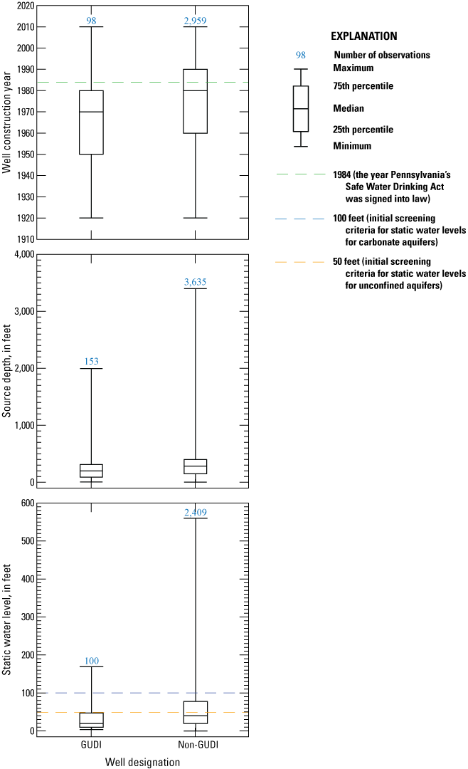
Comparison of public water-supply system well construction year, source depth, and static water level between wells classified as groundwater source under the direct influence of surface water (GUDI) and wells classified as non-GUDI.
Kruskal-Wallis test results showed significant differences in median values for construction year and casing depth between wells with MPA total risk-factor scores exceeding 0 and wells with MPA total risk-factor scores of zero (p <0.05); wells with MPA total risk-factor scores exceeding 0 had older median construction years and shallower casing depths (fig. 9). Similarly, Sharek (1998) examined well age as a contributor to high MPA risk indices, and the study concluded that newer wells use more improved materials than those available for construction of older wells and generally are subject to more stringent, modern construction standards. Therefore, deterioration associated with increased age of a well is also a factor that would contribute to a greater vulnerability and higher risk of contamination. Likewise, Nnadi and Sharek (1999) found that MPA total risk-factor scores generally increased with well age. Also, Sharek (1998) collected and analyzed samples and investigated characteristics of 62 wells in 7 Florida counties to determine contributors to high- and moderate-risk MPA results and found that wells with deeper casings had lower MPA risk indices, whereas wells with larger diameters had higher MPA risk indices due to the higher capacity of water that can be pumped from the well. Kozar and Paybins (2016) found that wells with casings deeper than 45 feet below the land surface had less bacterial contamination than wells with shorter casings.
Well construction characteristics did not differ significantly between wells that had moderate- or high-risk MPAs and wells that had low-risk MPAs. Also, data for well construction characteristics were insufficient to analyze wells in relation to categorical MPA total risk-factor scores according to major aquifer type, since only 53 wells had moderate- or high-risk MPAs, with that number decreasing further upon being divided according to four major aquifers. Differences in well-construction characteristics between wells with MPA total risk-factor scores exceeding zero and those with scores of zero were also analyzed according to carbonate and siliciclastic aquifers and yielded the same results discussed for all aquifer types. Differences in well characteristics were not analyzed for crystalline or surficial aquifers because each of these settings had less than 30 wells with MPA total risk-factor scores exceeding zero. No significant differences were found for wells with MPA total risk-factor scores exceeding zero whether they were completed in carbonate or siliciclastic aquifers.
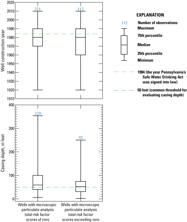
Comparison of well construction year and casing depth between wells with Microscopic Particulate Analysis (MPA) total risk-factor scores exceeding zero and wells with MPA total risk-factor scores of zero.
Pennsylvania Drinking Water Information System Database Subset
Data from the PADWIS database subset, consisting of information for 4,018 wells, were analyzed using Spearman’s rho to evaluate the statistical significance of correlations between: (1) the designation of a community well as GUDI, and (2) well-characteristic (table 1), spatial (table 2), and criteria (table 6) variables. Correlations between variables that were statistically significant (p <0.0001) and with Spearman’s rho values greater than or equal to 0.1 or less than or equal to −0.1 are indicated in table 8. Of the 10 well-characteristic variables, a total of 3 had a statistically significant (p <0.0001) correlation with a well being designated as GUDI and had Spearman’s rho values greater than or equal to 0.1 or less than or equal to −0.1 (table 8). From the well-characteristic variables, aquifer confinement and average well yield had positive correlations for a well designated as GUDI, whereas static water level was negatively correlated with a well designated as GUDI. These findings indicate that wells designated as GUDI may be present in unconfined aquifers and have high average yield and shallow static water levels relative to the non-GUDI wells.
Table 8.
Spearman’s rho correlations for well-characteristic data and criteria variable data that have the best correlations with a well being designated as groundwater under the direct influence of surface water (GUDI).[only includes results with p less than 0.0001 and rho greater than or equal to 0.10 or less than or equal to −0.10]
| Variable | Variable description | Variable type | Number of wells | Spearman's rho |
|---|---|---|---|---|
| NC | Northcentral region (1 = in region, 0 = all other) | Spatial | 4,018 | 0.41 |
| CONFINED | Description of aquifer indicating if it is confined, semi-confined, or unconfined (confined = 1, semi-confined = 2, unconfined = 3) | Well characteristic | 1,575 | 0.27 |
| UNC50 | Unconfined aquifers with a static water level less than or equal to 50 feet below the land surface | Criteria | 1,393 | 0.16 |
| RVCARB | Carbonate major aquifer types in the Ridge and Valley physiographic province (1 = Ridge and Valley, 0 = all other) | Spatial | 4,018 | 0.16 |
| NUMCRITERIAMET | Number of criteria met (between 0 and 7) from table 5 | Criteria | 2,855 | 0.14 |
| CARB | Carbonate major aquifer type (1 = carbonate, 0 = all other) | Spatial | 4,018 | 0.14 |
| CARBLE100 | Carbonate aquifers with a static water level less than or equal to 100 feet below the land surface | Criteria | 2,509 | 0.13 |
| AVG YIELD (GPD) | Source average yield, in gallons per day | Well characteristic | 2,127 | 0.11 |
| CONFNHD | Confined aquifers with an aquifer depth less than or equal to 50 feet below the land surface and located within 200 feet of a surface-water body | Criteria | 1,282 | −0.17 |
| NE | Northeast region (1 = in region, 0 = all other) | Spatial | 4,018 | –0.10 |
| SE | Southeast region (1 = in region, 0 = all other) | Spatial | 4,018 | –0.10 |
| STATIC WATER LEVEL (FT) | Source static water level, in feet | Well characteristic | 2,509 | –0.10 |
| SIL | Siliciclastic major aquifer type (1 = carbonate, 0 = all other) | Spatial | 4,018 | –0.10 |
Six of the 37 spatial variables were statistically significant (p <0.0001) with Spearman’s rho values greater than or equal to 0.1 or less than or equal to −0.1 (table 8). The NE, SE, and SIL spatial variables had a negative relation with a well being designated as GUDI, which illustrates that wells assumed to be drilled in siliciclastic aquifers in the Northeast or Southeast PADEP regions have decreased potential of being designated as GUDI. This finding coincides with conclusions drawn by Lindsey and Bickford (1999), who noted that of the major aquifer types in Pennsylvania, siliciclastic aquifers generally have a lesser potential for leaching of contaminants into groundwater than do aquifers underlain by other bedrock types. In addition, the CARB, RVCARB, and NC spatial variables had positive correlations with a well being designated as GUDI, indicating that wells assumed to be drilled in carbonate aquifers are especially vulnerable to contamination from land-surface run-off (Bickford and others, 1996; Embrey and Runkle, 2006; Fishel and Lietman, 1986; Lindsey and others, 2006; Lindsey and others, 2009).
Also, four of the eight criteria variables were statistically significant (p <0.0001) with Spearman’s rho values of at least 0.10 (table 8). Wells completed in unconfined aquifers with static water levels less than or equal to 50 feet below the land surface (UNC50; table 6) and wells completed in carbonate aquifers with static water levels less or equal to 100 feet below the land surface (CARBLE100; table 6) had positive correlations with a well being designated as GUDI, and wells in confined aquifers with an aquifer depth less than or equal to 50 feet below the land-surface and located within 200 feet of a surface-water body (CONFNHD; table 6) had negative correlations with a well being designated as GUDI. Interestingly, the aquifer depth PADWIS attribute (AQUIFER DEPTH [FT]; table 1) used to create the statistically significant CONFNHD criteria variable (table 6) did not have a statistically significant correlation with a well being designated as GUDI. Also, the total number of the seven criteria (NumCriteriaMet; table 6) that are met by wells had a positive correlation with a well being designated as GUDI. Overall, these findings for the criteria variables are similar to those illustrated by the PADWIS attributes, which is expected because the criteria variables were created primarily on the basis of PADWIS attributes.
Microscopic Particulate Analysis Database Subset
The MPA database subset, consisting of 631 community and non-community wells, was examined to determine the significance of variables to the MPA total risk-factor score for each well. Ten well-characteristic variables (table 1), 37 spatial variables (table 2), 13 water-quality parameters associated with MPA sample collection, and 23 bioindicator variables associated with MPA results were analyzed using Spearman’s rho to assess correlation significance between these variables and the MPA total risk-factor scores and assigned hazard-level score (1-low, 2-moderate, 3-high).
Spearman’s rho computation was performed on rank-transformed water-quality variables rather than on actual values because the computation of this nonparametric statistic can include concentrations reported as less than the minimum reporting level (MRL). This enabled the use of all the data in nonparametric statistical analyses without making assumptions about the distribution of values less than the MRL, below the lower limit, or above the upper limit for the explanatory variables further described here (Helsel and Hirsch, 2002). Analytical results for nitrate, sulfate, and turbidity had MRLs of 0.04 mg/L, 15 and 20 mg/L, and 0.3 and 0.5 Nephelometric Turbidity Units, respectively. Reported nitrate concentrations below the MRL, reported sulfate concentrations below the highest MRL, and turbidity values below the highest MRL were censored to the highest MRL associated with each constituent or property. This enabled the use of all the data in nonparametric statistical analyses without making assumptions about the distribution of the data below the MRL for nitrate, sulfate, or turbidity (Helsel and Hirsch, 2002). Results of analyses for E. coli and total coliform were quantified with both less-than and greater-than values, bounding the data at upper and lower limits, whereas results of analyses for fecal coliform were quantified with greater-than values, bounding the data at an upper limit. E. coli results were quantified with less-than values of 0 and 1 CFU/100 mL and a greater-than value of 200 CFU/100 mL; total coliform results were quantified with less-than values of 0 and 1 CFU/100 mL and 6 greater-than values ranging from 80 to 2,400 CFU/100 mL; fecal coliform results were quantified with greater-than values of 60 and 200 CFU/100 mL. Analytical results for these three bacteria species were censored to the highest lower limit (1 CFU/100 mL for E. coli and total coliform) and the lowest upper limit (200, 80, and 60 CFU/100 mL for E. coli, total coliform, and fecal coliform, respectively) associated with each constituent. For MPA result bioindicator counts, counts of diatoms, coccidia, other algae, rotifers, and plant debris were quantified with greater-than values of 150, 300, 150, and 150 and 200, respectively, bounding the data at an upper count limit. Counts of bioindicators greater than these upper count limits were censored to the lowest associated value for each upper count limit for each parameter. Those variables that were statistically significant (p <0.0001) and had Spearman’s rho values greater than or equal to 0.1 or less than or equal to −0.1 are indicated in table 9.
Table 9.
Spearman’s rho correlations for well-characteristic, water-quality, spatial, and bioindicator data that have the best correlations with Microscopic Particulate Analysis (MPA) total risk-factor scores and assigned hazard-level scores.[MPA, Microscopic Particulate Analysis; NS, not significant (p equal to or greater than 0.0001 and (or) rho less than 0.10 and greater than −0.10)]
Of the 10 well-characteristic variables, only one had a correlation with MPA total risk-factor score that was statistically significant (p <0.0001) with a Spearman’s rho value less than -0.10 (table 9). The aquifer depth variable, which describes the depth to the major water-bearing zone, had a negative correlation with MPA total risk-factor scores, suggesting that wells completed in aquifers with depths closer to the land-surface (shallower and relatively younger groundwater) had higher MPA total risk-factor scores than wells completed in aquifers with depths further from the land-surface (deeper and relatively older groundwater). Of the 37 spatial variables, two geologic variables (CARB and RVCARB; table 2) had statistically significant (p <0.0001) Spearman’s rho correlations. The statistical significance of wells completed in carbonate aquifers, especially in the Ridge and Valley Province, indicated that these aquifers are especially vulnerable to contamination and MPA samples with high total risk-factor and hazard-level scores.
Of the 13 water-quality parameters analyzed, fecal coliform and coliform had statistically significant positive correlations with both MPA total risk-factor scores and assigned hazard-level scores (table 9). Also, out of the 23 bioindicator variables analyzed, 17 had statistically significant positive correlations with MPA total risk-factor scores, while 20 had statistically significant positive correlations with assigned hazard-level scores. Of the bioindicator variables, the risk-factor score, sample count, and presence or absence variables for algae, rotifers, and diatoms had the highest positive correlations with both MPA total risk-factor scores and assigned hazard-level scores, suggesting that these bioindicators are more commonly present in MPA samples with high risk-factor and hazard-level scores than bioindicators such as insects/crustacea, plant debris, giardia, or coccidia. These results highlight those bioindicators that are more commonly found in Pennsylvania groundwater as part of the SWIP and those bioindicator variables that best correspond with MPA samples with high total risk-factor and hazard-level scores and thus could influence the designation of a well as GUDI.
Limitations of the Data
Based on the analyses of data described in this report, broad conclusions are drawn regarding site-specific well characteristics and anthropogenic and naturogenic factors that were responsible for a well being designated as GUDI, but the accuracy of these analyses is dependent on the quality of the data. As previously explained, detailed case-file review showed the SWIP steps were typically utilized to generate data needed to evaluate wells, but for some wells the evaluation approach was based on other factors such as complex physical setting or other available data that could not be easily summarized in a database such as PADWIS.
In addition, analysis of the PADWIS database showed differences among regions in compiling data describing well characteristics and site-specific attributes. Some of the PADWIS database attributes were poorly populated (table 1). Other site-specific well characteristics used in the initial screening assessment, including: (1) presence of a documented surface-water recharge boundary, (2) proximity to a man-made feature that exposed the aquifer, and (3) well-construction deficiencies, were either not available or populated in the PADWIS database. The PADWIS database also did not provide important data attributes used in making GUDI determinations, such as distance from a well to the nearest hydrologic feature, Pearson-correlation coefficients calculated from 5-day averages of data collected during SWIP monitoring, and MPA results. Including Pearson-correlation coefficients calculated by PADEP during the SWIP as an attribute in the PADWIS database could be useful for understanding why a well was classified as GUDI. The correlation could be included as a categorical variable with designations, such as “none,” “low,” “moderate,” or “high,” indicating the strength of the correlation. Alternatively, the r-square value describing the correlation could be included with a note indicating the two variables that the correlation is describing. Results associated with MPA were an important, and often determinate, part of the SWIP because these results indicated how prevalent contaminants were and how easy it was for them to migrate into the water source. Therefore, it would be useful to include the numerical score and (or) risk classification resulting from a collected MPA sample as attribute(s) in the PADWIS database.
Detailed review of the files for specific wells indicated there were some differences between well files and the corresponding well record in the PADWIS database, which might have contributed to an inaccurate transfer of data. For example, investigation of files for wells in the Southcentral region indicated that well and casing depth records were sometimes inconsistent with the data values stored in the PADWIS database. In addition, spatial coordinates for 9 out of 11 wells further examined in the Southcentral region differed from spatial coordinates provided in the PADWIS database from 130 to 14,800 feet. Determination of well attributes using spatial data (such as computing distance to the nearest surface-water feature) relies on the accuracy of the spatial coordinates associated with the well in the PADWIS database. This introduces a major limitation in the usage of spatial data for GUDI determination and analysis of geographic characteristics compiled for wells because they were not available in the PADWIS database and could contribute to inaccuracy in significance of the Spearman’s rho correlation.
Summary
Several approaches were followed to evaluate the data and methodology used to identify groundwater sources in Pennsylvania that are under the direct influence of surface water (GUDI). The evaluation included file review, database quality control (QC), creation of database subsets, and statistical analyses of the data in those subsets. Most of the data were provided by the Pennsylvania Department of Environmental Protection (PADEP), including source data derived from PADEP case files, a source-information database for public water-supply systems, and Microscopic Particulate Analysis (MPA) results and associated water-quality data for public water-supply wells.
PADEP case files for 43 wells from the Department’s Northcentral and Southcentral regions were reviewed to gain a better understanding of how the surface-water identification protocol (SWIP) used by PADEP was applied in practice, to verify and compile missing data, and to find additional attributes not previously available that might explain a well's susceptibility to surface-water influence. Review of file information from these 43 wells showed that, for some sources, the GUDI determination is too complex to be easily summarized in a database. File review also showed that complex physical setting and available site-specific data may influence all three steps of the SWIP, but the effect on GUDI determination is difficult to quantify.
The PADWIS database, which consists of PADEP source-information data for public water-supply systems, contains files for 12,147 wells, 335 of which are classified as GUDI and 11,812 as non-GUDI. A subset of the PADWIS database consisting of 4,018 wells—176 GUDI wells and 3,842 non-GUDI wells—was created for analysis. The PADWIS database subset included only community wells for which the SWIP was used by PADEP to make GUDI determinations. MPA results for 631 community and non-community wells were compiled, along with data for associated water-quality constituents and properties (including alkalinity, chloride, Escherichia coli, fecal coliform, nitrate, pH, sodium, specific conductance, sulfate, total coliform, total dissolved solids, total residue, and turbidity) populated from the PADEP Bureau of Laboratories, Sample Information System. Data describing associated water-quality constituents and properties were available for varying amounts (between 49 to 367) of the 631 wells that had MPA results. Data obtained from sources other than PADEP include spatial data, both naturogenic (for example, average precipitation or distance to closest hydrologic feature) and anthropogenic (for example, percentage of developed or agricultural land cover within a specific vicinity of a well).
Data describing the major aquifer type in which a well is completed, the physiographic province in which it is located, and construction data for wells in the PADWIS database subset and MPA database subset were analyzed using the Kruskal-Wallis test to evaluate differences among groups. For the PADWIS dataset subset, GUDI wells had significantly older median construction years, shallower well depths, and static water levels closer to the land surface than non-GUDI wells. Assessment of the MPA database subset showed wells with MPA total risk-factor scores exceeding zero had older median construction years and shallower depths to the bottom of the casing than wells with MPA total risk-factor scores of zero. The highest percentages of wells designated as GUDI (12 percent) and with MPA total risk-factor scores exceeding 0 (30 percent) were completed in carbonate aquifers, whereas the least number of wells designated as GUDI (1 well) and with MPA total risk-factor scores exceeding zero (23 wells) were completed in crystalline aquifers.
Spearman’s rank correlation coefficient (rho) was used to characterize available data that best identify a community well as being GUDI or a community or non-community well with a contaminated MPA result, which could potentially be the cause of a GUDI determination. Analysis of the PADWIS database subset using Spearman’s rho illustrated that community wells designated as GUDI occur in unconfined aquifers and have high average yield and shallow static water levels. Wells completed in unconfined aquifers with static water levels less than or equal to 50 feet below the land surface and wells in carbonate aquifers with static water levels less than or equal to 100 feet below the land surface were positively correlated with a GUDI well designation. Wells completed in confined aquifers at depths less than or equal to 50 feet below the land surface and located within 200 feet of a surface-water body had negative correlations with a well being designated as GUDI. Also, wells drilled in siliciclastic major aquifers (SIL) and within PADEP’s Northeast (NE) or Southeast (SE) regions had a negative relation with a GUDI designation. Results indicated that wells in PADEP’s Northcentral (NC) region and that are completed in carbonate aquifers (CARB), especially within the Ridge and Valley Province (RVCARB), have increased probability of being designated as GUDI. The PADEP region variables illustrate potential affects that a complex physical setting and available site-specific data can have on the implementation of a uniform evaluation approach for GUDI across the state.
The MPA database subset was also examined to determine the significance of associated well-characteristic variables, spatial variables, bioindicator counts and scores, and water-quality results in relation to resulting MPA total risk-factor scores and assigned hazard-level scores (1-low, 2-moderate, 3-high). Spearman’s rho correlations showed that wells completed in carbonate aquifers, especially within the Ridge and Valley Province and with depths closer to the land-surface, had higher total risk-factor scores resulting from MPA samples. Fecal coliform and coliform had statistically significant positive correlations with both MPA total risk-factor scores and assigned hazard-level scores. Of the bioindicator variables, the risk-factor score, sample count, and presence or absence variables for algae, rotifers, and diatoms had the highest positive correlations with both MPA total risk-factor scores and assigned hazard-level scores, suggesting that these bioindicators are more commonly present in MPA samples with high risk-factor and hazard-level scores than bioindicators such as insects/crustacea, plant debris, giardia, or coccidia.
Based on the results of the analyses described in this report, broad conclusions can be drawn regarding site-specific well characteristics and anthropogenic and naturogenic factors that could be responsible for a well being designated as GUDI, but the accuracy of these results is dependent on the quality of the data being analyzed. Detailed review of well files showed that the SWIP steps are usually followed, but for some sources, the GUDI determination in practice is more complex than what can be easily summarized in the PADWIS database. Some critical site-specific well characteristics used in the SWIP either are not available or not populated in the PADWIS database. Detailed file review for specific wells showed data discrepancies between well files and the corresponding well record in the PADWIS database, including discrepancies between critical attributes such as well depth, well casing depth, and well spatial coordinates. These inaccuracies have the potential to cause major limitations in the usage of spatial data for population and analysis of geographic characteristics not available in the PADWIS database and could contribute to inaccuracy in the statistical correlations. These results, however, still serve to highlight statewide complexities related to determining a representative source classification and the need for further field-scale investigation.
References Cited
Ayotte, J.D., Cahillane, M., Hayes, L., and Robinson, K.W., 2012, Estimated probability of arsenic in groundwater from bedrock aquifers in New Hampshire, 2011: U.S. Geological Survey Scientific Investigations Report 2012–5156, 25 p., accessed December 19, 2012, at https://pubs.usgs.gov/sir/2012/5156/.
Bickford, T.M., Lindsey, B.D., and Beaver, M.R., 1996, Bacteriological quality of ground water used for household supply, Lower Susquehanna River Basin, Pennsylvania and Maryland: U.S. Geological Survey Water-Resources Investigations Report 96–4212, 31 p., accessed March 21, 2018, at https://doi.org/10.3133/wri964212.
Braun, D.D., 2004, The glaciation of Pennsylvania, USA, in Ehlers, J., and Gibbard, P.L., eds., Quaternary glaciations—Extent and chronology [Part 2—North America], Developments in Quaternary Sciences: Amsterdam, Elsevier, p. 237–242. [Also available at https://doi.org/10.1016/S1571-0866(04)80201-X.]
Centers for Disease Control and Prevention, 2015, Parasites: Centers for Disease Control and Prevention, National Center for Emerging and Zoonotic Infections Diseases, Division of Foodborne, Waterborne, and Environmental Diseases, accessed July 18, 2017, at https://www.cdc.gov/parasites/.
Craun, G.F., Hubbs, S.A., Frost, F., Calderon, R.L., and Via, S.H., 1998, Waterborne outbreaks of cryptosporidiosis: Journal—American Water Works Association, v. 90, no. 9, p. 81–91. [Also available at https://doi.org/10.1002/j.1551-8833.1998.tb08500.x.]
Daly, C., Gibson, W.P., Taylor, G.H., Johnson, G.L., and Pasteris, P., 2002, A knowledge-based approach to the statistical mapping of climate: Climate Research, v. 22, p. 99–113, accessed February 7, 2018, https://doi.org/10.3354/cr022099.
Eberts, S.M., Thomas, M.A., and Jagucki, M.L., 2013, The quality of our Nation’s waters—Factors affecting public-supply-well vulnerability to contamination—Understanding observed water quality and anticipating future water quality: U.S. Geological Survey Circular 1385, 120 p., accessed November, 16, 2018, at https://pubs.usgs.gov/circ/1385/.
Embrey, S.S., and Runkle, D.L., 2006, Microbial quality of the Nation’s ground-water resources, 1993–2004: U.S. Geological Survey Scientific-Investigations Report 2006–5290, 34 p., accessed March 21, 2018, at https://pubs.usgs.gov/sir/2006/5290/.
Fishel, D.K., and Lietman, P.L., 1986, Occurrence of nitrate and herbicides in ground water in the Upper Conestoga River Basin, Pennsylvania: U.S. Geological Survey Water-Resources Investigations Report 85–4202, 8 p. [Also available at https://doi.org/10.3133/wri854202.]
Gollnitz, W.D., Clancy, J.L., and Garner, S.C., 1997, Reduction of microscopic particulates by aquifers: Journal - American Water Works Association, v. 89, no. 11, p. 84–93, accessed December 10, 2014, at https://doi.org/10.1002/j.1551-8833.1997.tb08324.x.
Gross, E.L., 2022, Database used for the evaluation of data used to identify groundwater sources under the direct influence of surface water in Pennsylvania: U.S. Geological Survey data release, https://doi.org/https://doi.org/10.5066/P9Q0BXH1.
Helsel, D.R., and Hirsch, R.M., 2002, Statistical methods in water resources: U.S. Geological Survey Techniques of Water-Resources Investigations, book 4, chap. A3, 522 p., accessed June 16, 2016, at https://pubs.usgs.gov/twri/twri4a3/.
Johnson, G.C., Zimmerman, T.M., Lindsey, B.D., and Gross, E.L., 2011, Factors affecting groundwater quality in the Valley and Ridge aquifers, eastern United States, 1993–2002: U.S. Geological Survey Scientific Investigations Report 2011–5115, 70 p., accessed August 1, 2011, at https://doi.org/10.3133/sir20115115.
Knobel, L.L., Chapelle, F.H., and Meisler, H., 1998, Geochemistry of the Northern Atlantic Coastal Plain aquifer system: U.S. Geological Survey Professional Paper 1404–L, 57 p., accessed March 21, 2018, at https://doi.org/10.3133/pp1404L.
Kozar, M.D., and Paybins, K.S., 2016, Assessment of hydrogeologic terrains, well-construction characteristics, groundwater hydraulics, and water-quality and microbial data for determination of surface-water-influenced groundwater supplies in West Virginia (ver. 1.1, October 24, 2016): U.S. Geological Survey Scientific Investigations Report 2016–5048, 54 p., accessed April 25, 2017, at https://doi.org/10.3133/sir20165048.
Lindsey, B.D., and Bickford, T.M., 1999, Hydrogeologic framework and sampling design for an assessment of agricultural pesticides in ground water in Pennsylvania: U.S. Geological Survey Water-Resources Investigations Report 99–4076, 44 p., accessed February 6, 2014, at https://pubs.usgs.gov/wri/1999/4076/wri19994076.pdf.
Lindsey, B.D., Berndt, M.P., Katz, B.G., Ardis, A.F., and Skach, K.A., 2009, Factors affecting water quality in selected carbonate aquifers in the United States, 1993–2005: U.S. Geological Survey Scientific Investigations Report 2008–5240, 117 p., accessed February 7, 2018, at https://doi.org/10.3133/sir20085240.
Lindsey, B.D., Falls, W.F., Ferrari, M.J., Zimmerman, T.M., Harned, D.A., Sadorf, E.M., and Chapman, M.J., 2006, Factors affecting occurrence and distribution of selected contaminants in ground water from selected areas in the Piedmont Aquifer System, eastern United States, 1993–2003: U.S. Geological Survey Scientific Investigations Report 2006–5104, 72 p., accessed February 7, 2018, at https://doi.org/10.3133/sir20065104.
Lindsey, B.D., Rasberry, J.S., and Zimmerman, T.M., 2002, Microbiological quality of water from noncommunity supply wells in carbonate and crystalline aquifers of Pennsylvania: U.S. Geological Survey Water-Resources Investigations Report 2001–4268, 30 p., accessed May 9, 2017, at https://doi.org/10.3133/wri014268.
Llewellyn, G.T., 2014, Evidence and mechanisms for Appalachian Basin brine migration into shallow aquifers in [Northeastern] Pennsylvania, USA: Hydrogeology Journal, v. 22, no. 5, p. 1055–1066, accessed June 16, 2016, at https://doi.org/10.1007/s10040-014-1125-1.
Nnadi, F.N., and Fulkerson, M., 2002, Assessment of groundwater under direct influence of surface water: Journal of Environmental Science and Health. Part A, Toxic/Hazardous Substances & Environmental Engineering, v. 37, no. 7, p. 1209–1222, accessed December 15, 2016, at https://doi.org/10.1081/ESE-120005981.
Nnadi, F.N., and Sharek, R.C., 1999, Factors influencing groundwater sources under the direct influence of surface waters: Journal of Environmental Science and Health. Part A, Toxic/Hazardous Substances & Environmental Engineering, v. 34, no. 1, p. 201–215, accessed December 15, 2016, at https://doi.org/10.1080/10934529909376831.
Olson, M.E., O’Handley, R.M., Ralston, B.J., McAllister, T.A., and Andrew Thompson, R.C., 2004, Update on Cryptosporidium and Giardia infections in cattle: Trends in Parasitology, v. 20, no. 4, p. 185–191, accessed December 15, 2016, at https://doi.org/10.1016/j.pt.2004.01.015.
Pennsylvania Bureau of Topographic and Geologic Survey, 2007, Digital data set of mapped karst features in south-central and southeastern Pennsylvania: Pennsylvania Bureau of Topographic and Geologic Survey, Department of Conservation and Natural Resources online database, accessed June 16, 2017, at https://www.pasda.psu.edu/uci/DataSummary.aspx?dataset=3073.
Pennsylvania Bureau of Topographic and Geologic Survey, 2008, Physiographic provinces: Pennsylvania Bureau of Topographic and Geologic Survey, Department of Conservation and Natural Resources online database, accessed February 26, 2009, at https://www.pasda.psu.edu/uci/DataSummary.aspx?dataset=1153.
Pennsylvania Department of Environmental Protection, 2000, DEP regions: Pennsylvania Department of Environmental Protection online database, accessed December 6, 2016, at https://www.pasda.psu.edu/uci/DataSummary.aspx?dataset=1089.
Pennsylvania Department of Environmental Protection, 2001, Guidance for surface water identification protocol: Pennsylvania Department of Environmental Protection, Bureau of Water Supply Management, Technical Guidance Document 383–3500–106, 34 p., accessed March 16, 2016, at https://mdw.srbc.net/pwsap/Spring2016Workshops/assets/docs/0845%20-%20PADEP%20-%20Safe%20Drinking%20Water%20Program/PADEP%20References/383-3500-106_Gu idance%20for%20Surface%20Water%20Protocol.pdf.
Pennsylvania Department of Environmental Protection, 2002a, Surface water identification protocol—Noncommunity water systems: Pennsylvania Department of Environmental Protection, Bureau of Water Supply and Wastewater Management, Technical Guidance Document 383–3500–112, 8 p., accessed March 16, 2016, at http://www.depgreenport.state.pa.us./elibrary/GetDocument?docld=7436&DocName=SURFACE%20WATER%20IDENTIFICATION%20PROTOCOL-NONCOMMUNITY%20WATER%20SYSTEM S.PDF%20%20%3Cspan%20style%3D%22color%3Agreen%3B%22%3E%3C%2Fspan%3E%20%3Cspan%20style%3D%22color%3Ablue%3B%22%3E%3C%2Fspan%3E.
Pennsylvania Department of Environmental Protection, 2002b, Summary of key requirements for surface water identification protocol: Pennsylvania Department of Environmental Protection, Bureau of Water Supply and Wastewater Management, Technical Guidance Document 383–0810–206, 14 p., accessed December 15, 2016, at http://www.depgreenport.state.pa.us/elibrary/GetDocument?docID=7647&DocName=SUMMARY%20OF%20KEY%20REQUIREMENTS%20FOR%20SURFACE%20WATER%20IDENTIFICATION %20PROTOCOL.PDF%20%20%3Cspan%20style%3D%22color%3Agreen%3B%22%3E%3C%2Fspan%3E%20%3Cspan%20style%3D%22color%3Ablue%3B%22%3E%3C%2Fspan%3E.
Pennsylvania Department of Environmental Protection, 2015, Pennsylvania public water system compliance report for 2015: Pennsylvania Department of Environmental Protection, accessed January 13, 2017, at https://files.dep.state.pa.us/Water/BSDW/DrinkingWaterManagement/PA_DEP_2015_Annual_Compliance_Report.pdf.
Pennsylvania Department of Environmental Protection, 2018, Regional resources: Pennsylvania Department of Environmental Protection web page, accessed February 7, 2018, at https://www.dep.pa.gov/About/Regional/Pages/default.aspx.
PRISM Climate Group, 2006, United States average monthly or annual precipitation, 1971–2000: Oregon State University, digital data, accessed May 19, 2009, at http://www.prism.oregonstate.edu/products/matrix.phtml?vartype=ppt&view=data.
Rogers, R.J., 1989, Geochemical comparison of ground water in areas of New England, New York, and Pennsylvania: Ground Water, v. 27, no. 5, p. 690–712, accessed February 7, 2018, at https://doi.org/10.1111/j.1745-6584.1989.tb00483.x.
Sharek, R.C., 1998, Well characteristics influencing microscopic particulate analysis risk index: Orlando, Fla., University of Central Florida, M.S. thesis, 186 p., accessed March 15, 2018, at https://stars.library.ucf.edu/rtd/2533/.
Trapp, H., Jr., and Horn, M.A., 1997, Ground water atlas of the United States—Segment 11: Delaware, Maryland, New Jersey, North Carolina, Pennsylvania, Virginia, West Virginia, U.S. Geological Survey Hydrologic Investigations Atlas 730–L., 24 p., accessed March 21, 2018, at https://doi.org/10.3133/ha730L.
U.S. Bureau of the Census, 2000, 2000 county [and] county equivalent areas: U.S. Bureau of the Census, digital data, accessed June 11, 2008, at https://www.census.gov/geo/maps-data/data/cbf/cbf_counties.html.
U.S. Environmental Protection Agency, 1992, Consensus method for determining groundwaters under the direct influence of surface water using microscopic particulate analysis: U.S. Environmental Protection Agency, EPA–910/9–92–029, 53 p., accessed September 9, 2016, at https://nepis.epa.gov/Exe/ZyNET.exe/P100C58D.TXT?ZyActionD=ZyDocument&Client=EPA&Index=1991+Thru+1994&Docs=&Query=&Time=&EndTime=&SearchMethod=1&TocRe strict=n&Toc=&TocEntry=&QField=&QFieldYear=&QFieldMonth=&QFieldDay=&IntQFieldOp=0&ExtQFieldOp=0&XmlQuery=&File=D%3A%5Czyfiles%5CIndex%20Data%5C91thru9 4%5CTxt%5C00000026%5CP100C58D.txt&User=ANONYMOUSE&Password=anonymous&SortMethod=h%7C-&MaximumDocuments=1&FuzzyDegree=0&ImageQuality=r75g8/r75g8/x150y1 50g16/i425&Display=hpfr&DefSeekPage=x&SearchBack=ZyActionL&Back=ZyActionS&BackDesc=Results%20page&MaximumPages=1&ZyEntry=1&SeekPage=x&ZyPURL.
U.S. Geological Survey, 2009, 1-Arc second national elevation dataset: U.S. Geological Survey, raster digital data, accessed September 8, 2009, at http://seamless.usgs.gov/index.php.
U.S. Geological Survey, 2014a, NHD_M_42_Pennsylvania_ST: U.S. Geological Survey, vector digital data, accessed November 18, 2016, at ftp://rockyftp.cr.usgs.gov/vdelivery/Datasets/Staged/Hydro/Shape/NHD_M_42_Pennsylvania_ST.zip.
U.S. Geological Survey, 2014b, National land cover database 2011 land cover (2011 ed.): U.S. Geological Survey, accessed April 12, 2016, at https://www.usgs.gov/media/images/nlcd-2011-land-cover-2011-edition-amended-2014.
Winter, T.C., Harvey, J.W., Franke, O.L., and Alley, W.M., 1998, Ground water and surface water—A single resource: U.S. Geological Survey Circular 1139, 79 p., accessed September 20, 2020, at https://pubs.er.usgs.gov/publication/cir1139.
Wolock, D.M., 1997, STATSGO soil characteristics for the conterminous United States: U.S. Geological Survey Open-File Report 656, accessed May 28, 2008, at https://water.usgs.gov/GIS/metadata/usgswrd/XML/muid.xml.
Wolock, D.M., 2003, Estimated mean annual natural ground-water recharge in the conterminous United States: U.S. Geological Survey, accessed May 28, 2008, at https://water.usgs.gov/GIS/metadata/usgswrd/XML/rech48grd.xml.
Conversion Factors
Datum
Vertical coordinate information is referenced to the North American Vertical Datum of 1988 (NAVD 88).
Horizontal coordinate information is referenced to the North American Datum of 1983 (NAD 83).
Elevation, as used in this report, refers to distance above the vertical datum.
Supplemental Information
Specific conductance is given in microsiemens per centimeter at 25 degrees Celsius (µS/cm at 25 °C).
Concentrations of chemical constituents in water are given in either milligrams per liter (mg/L) or micrograms per liter (µg/L).
Abbreviations
°C
degrees Celsius
BOL
Bureau of Laboratories
CFU/100 mL
colony forming units per 100 milliliters
E. coli
Escherichia coli
EPA
U.S. Environmental Protection Agency
GIS
geographic information system
GUDI
groundwater source under the direct influence of surface water
mg/L
milligram per liter
MPA
Microscopic Particulate Analysis
non-GUDI
groundwater source not under the direct influence of surface water
NLCD
National Land Cover Database
PADEP
Pennsylvania Department of Environmental Protection
PADWIS
Pennsylvania Drinking Water Information System
QC
quality control
SDWA
Safe Drinking Water Act
SWIP
Surface Water Identification Protocol
SWTR
Surface Water Treatment Rule
USGS
U.S. Geological Survey
For additional information, contact
Director, Pennsylvania Water Science Center
U.S. Geological Survey
215 Limekiln Road
New Cumberland, PA 17070
or visit our website at:
https://usgs.gov/centers/pa-water/
Publishing support provided by the West Trenton Publishing Service Center
Disclaimers
Any use of trade, firm, or product names is for descriptive purposes only and does not imply endorsement by the U.S. Government.
Although this information product, for the most part, is in the public domain, it also may contain copyrighted materials as noted in the text. Permission to reproduce copyrighted items must be secured from the copyright owner.
Suggested Citation
Gross, E.L., Conlon, M.D., Risser, D.W., and Reisch, C.E., 2022, Compilation and evaluation of data used to identify groundwater sources under the direct influence of surface water in Pennsylvania (ver. 2.0, June 2023): U.S. Geological Survey Open-File Report 2022–1023, 41 p., https://doi.org/10.3133/ofr20221023.
ISSN: 2331-1258 (online)
Study Area
| Publication type | Report |
|---|---|
| Publication Subtype | USGS Numbered Series |
| Title | Compilation and evaluation of data used to identify groundwater sources under the direct influence of surface water in Pennsylvania |
| Series title | Open-File Report |
| Series number | 2022-1023 |
| DOI | 10.3133/ofr20221023 |
| Edition | Version 1.0: May 2022; Version 2.0: June 2023 |
| Publication Date | May 09, 2022 |
| Year Published | 2022 |
| Language | English |
| Publisher | U.S. Geological Survey |
| Publisher location | Reston, VA |
| Contributing office(s) | Pennsylvania Water Science Center |
| Description | Report: viii, 38 p.; Data Release |
| Country | United States |
| State | Pennsylvania |
| Online Only (Y/N) | Y |
| Additional Online Files (Y/N) | N |