

Assessing the Efficacy of Using a Parentage-Based Tagging Survival Model to Evaluate Two Sources of Mortality for Juvenile Chinook Salmon (Oncorhynchus tshawytscha) in Lookout Point Reservoir, Oregon
Links
- Document: Report (1.9 MB pdf) , HTML , XML
- Download citation as: RIS | Dublin Core
Acknowledgments
Funding for this research was provided by the U.S. Army Corps of Engineers. Staff from Oregon State University provided information from recent studies on copepods in Willamette Basin reservoirs that was useful in this study, and we thank Dr. James Peterson, Travis Neal, and Dr. Christina Murphy for their insights. Data are not currently available from funding organization, the U.S. Army Corps of Engineers. Contact the U.S. Army Corps of Engineers for further information.
Abstract
We conducted a study to assess the efficacy of using a parentage-based tagging survival model (PBT N-mixture model) to evaluate two sources of mortality for juvenile Chinook salmon (Oncorhynchus tshawytscha) in Lookout Point Reservoir, Oregon. The model was originally developed to evaluate reservoir mortality because of predation from piscivorous fish. However, recent studies have also found that juvenile Chinook salmon experience high infection rates from parasitic copepods (Salmincola californiensis), which are known to negatively affect performance and survival. Our study was conducted to determine if the PBT N-mixture model could separately estimate mortality because of predation from non-native fish and mortality resulting from copepod infection. This assessment was conducted in two parts: (1) data collected in Lookout Point Reservoir during 2018 were re-analyzed; and (2) a simulation was conducted to evaluate a multi-year study that included inter-annual variation in copepod infection rate and two subsampling strategies (10 fish per month, 30 fish per month) to characterize monthly copepod infection rate. Results from each of these efforts suggest that the survival model is unlikely to provide reliable survival estimates for the two mortality sources that we evaluated. The re-analysis of 2018 data showed that “predation only” and “copepod only” models estimated a negative coefficient for the respective covariate, but the model that included both covariates provided coefficient estimates that differed from the other models and were highly uncertain. Similarly, the simulation results showed that most models failed to correctly estimate the magnitude and direction of mortality due to predation and copepods. These results suggest that additional data will be required if a model is desired that can separately estimate mortality effects due to both predation and copepods in the future. The existing data are limited by factors including low detection probabilities from previous field studies, existing uncertainties about copepod effects on mortality in a natural setting and expected limitations in the number of years that a field study could realistically be expected to receive funding.
Introduction
Estimates of survival for specific life-stages of Pacific salmon (Oncorhynchus spp.) are important data for resource managers in impounded river systems of the western United States. During the past 2 decades, techniques have been developed and refined to estimate survival of smolt and adult life stages. These techniques rely on data collected from fish marked with individually identifiable tags (passive integrated transponders [PIT tags]) or transmitters (radio and acoustic transmitters) and are generally applied to populations of actively migrating fish (Skalski and others, 1998, 201626; Muir and others, 2001; Perry and others, 2010). However, in places like the Willamette River, Oregon, resource managers need to understand survival patterns for subyearling Chinook salmon (Oncorhynchus tshawytscha), specifically those in the fry and parr life stages rearing in reservoirs. Estimation of survival for these life stages is challenging because fish are too small to be tagged with a PIT tag or an active transmitter, and methods for estimating survival of fish in this size class have not been tested and proven.
The U.S. Army Corps of Engineers (USACE) operates the Willamette Project (Project) in western Oregon, which includes 13 dams and reservoirs, approximately 68 kilometers of revetments, and several fish hatcheries. The primary purpose of the Project is flood risk management, but it is also operated to provide hydroelectricity, irrigation water, navigation, instream flows for wildlife, and recreation. The Project was determined to jeopardize Upper Willamette spring Chinook salmon and winter steelhead (Oncorhynchus mykiss; NOAA, 2008), which has spurred a series of studies and actions to reduce the Project’s impacts on these populations. Downstream, juvenile fish passage is one of the key issues in the Project. Passage for adult salmon and steelhead is accomplished using trap-and-haul methods which provides spawning opportunities in free-flowing headwaters and tributaries upstream of Project reservoirs (Sard and others, 2015). Progeny of the transported adults move downstream and spend several months rearing in Project reservoirs because passage options are currently (as of 2022) limited to spill, regulating outlets, and turbine passage at the high-head dams in the system (Keefer and others, 2013; Beeman and others, 2014; Kock and others, 2015; Monzyk and others, 2015a). Thus, fishery managers are faced with determining whether it is better to focus on developing fish passage options at dams or attempting to capture fish near the head of the reservoirs. A key piece of information that will help with these decisions is understanding survival rates of juvenile salmon rearing in reservoirs. High survival rates would likely result in decisions to focus on dam-based passage or collection efforts whereas low survival rates may result in decisions to focus on collecting fish as they enter the reservoirs.
The U.S. Geological Survey (USGS) developed a study design to estimate survival of juvenile Chinook salmon in Lookout Point Reservoir, located on the Middle Fork Willamette River, and completed 2 years of research and survival estimation in 2017 and 2018 (Kock and others, 2016, 2019a, b). These studies implemented a novel statistical model, the parentage-based tagging PBT N-mixture model, that uses genetic markers passed to progeny from known parental groups spawned in the hatchery to estimate survival of juvenile Chinook salmon too small to tag with conventional means. This model is described in detail in Kock and others (2019a, b). These studies were able to generate survival estimates during April–October each year, but survival trends differed between years; monthly survival probability estimates increased from April to October in 2017 but decreased during this same period in 2018 (fig. 1; Kock and others 2019a, b). The study design was originally conceived with the hypothesis that reservoir mortality of juvenile Chinook salmon would primarily result from predation by piscivorous fish species which have robust populations in Lookout Point Reservoir (Brandt and others, 2016; Murphy and others, 2021). However, recent studies have shown that Willamette Basin reservoirs support abundant populations of parasitic copepods (Salmincola californiensis), which negatively affect the performance and survival of juvenile Chinook salmon (Monzyk and other, 2015b; Herron and others, 2018; Murphy and others, 2020a; Neal and others, 2021). During the 2018 study, Kock and others (2019b) documented the proportion of juvenile Chinook salmon that were visually confirmed to be infected with copepods (fig. 2) during monthly collection efforts in their study, but this information was not used in survival analyses. Kock and others (2019b) concluded: “We lack data to definitively determine what factors resulted in different survival estimates between years, but reservoir conditions, fish distribution patterns, and emerging information on copepods warrant consideration.”
In response to the uncertainty about trends in survival in Lookout Point, we conducted additional analyses to determine if the PBT N-mixture model could separately estimate mortality because of predation from that of copepod infection. This study was conducted in two parts. In the first part, we reevaluated field data to determine whether separate effects of copepod infection and predation could be discerned with PBT N-mixture model. In the second part, we designed and implemented a simulation study to evaluate the ability of PBT N-mixture model to discern a trend with multiple years of data.
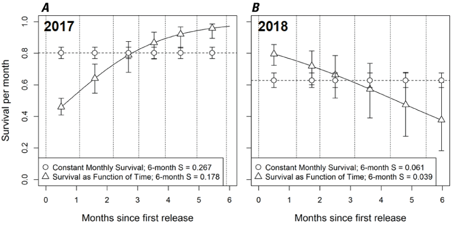
Monthly survival estimates for subyearling Chinook salmon (Oncorhynchus tshawytscha) in Lookout Point Reservoir during April (0)–October (6) (A) 2017 and (B) 2018. The survival (S) relation was estimated as constant monthly survival (open circles) and as a function of time-since-release (triangles) for each year. The inset legend provides estimates of total survival probability of 6 months. Symbols identify point estimates for survival and whiskers identify the 95-percent credible intervals of the point estimates.
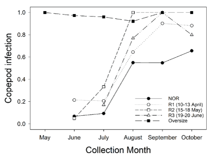
Proportion of juvenile Chinook salmon (Oncorhynchus tshawytscha) infected with the copepod Salmincola californiensis in Lookout Point Reservoir during May–October 2018. Figure was reprinted from Kock and others (2019b). Acronyms in the figure include the following: NOR = natural origin; R1 = release 1; R2 = release 2; R3 = release 3. Release dates are shown in parentheses for R1, R2, and R3.
Methods
Re-Analysis of 2018 Lookout Point Reservoir Data
Field data from Lookout Point Reservoir collected in 2018 were reanalyzed to determine whether mortality could be statistically attributed to two different sources. These data are described in detail in Kock and others (2019b). The two sources of mortality considered were (1) an index of sampling occasion (time) as a surrogate measure of reduced predation risk with increasing fish size and (2) adult copepod incidence rate in sampled fish. We did not attempt to model field data collected in 2017 because information on copepod infection was not collected. Adult copepod infection rate was the proportion of captured juvenile Chinook salmon with visible adult, female copepods attached averaged across release groups. The average across groups was used to reduce the number of parameters required in the model and thus increase power to detect an effect. Infection rate increased through time in 2018 from relatively low levels in June and July to very high levels (exceeding 90 percent) in September (fig. 2).
We hypothesized that the two sources of mortality should have countervailing effects. That is, absent any effect of copepod infection, monthly survival probability should increase over time because of decreased predation as juvenile Chinook salmon grew to larger sizes. Survival estimates from the 2017 field study supported this hypothesis as Kock and others (2019a) found support in the data for a positive trend in survival with increasing time (fig. 1A). Contrastingly, absent any effect of size-dependent predation, we hypothesized that survival should decrease with increasing copepod infection rates. Emerging evidence has demonstrated the potential for copepod infections to substantially decrease survival of juvenile Chinook salmon (Beeman and others, 2015; Herron and others, 2018, Neal and others, 2021). In particular, Neal and others (2021) demonstrated through laboratory-controlled infection of juvenile Chinook salmon that fish exposed to greater levels of copepod density and higher water temperatures experienced elevated mortality. The declining trend in monthly survival estimates from 2018 (Kock and others, 2019b; fig. 1B) coincident with rising copepod infection rates suggest that copepod induced mortality is a plausible explanation for the overserved trend.
We used the PBT N-mixture model previously described in Kock and others (2019a, b) to assess the support in the data for countervailing effects from these two covariates. We briefly review the structure of that model here. The model consists of two related equations:
and whereNik is the abundance of PBT family group i during primary sampling occasion k,
is the survival probability between primary sampling occasions k-1 to k,
is the probability that an individual from PBT family group i during primary sampling occasion k is first captured on the jth sample, and
is the number of individuals from PBT family group i collected in the jth sample during the kth primary sampling occasion.
The likelihood of the data given the survival and collection probability parameters and pjk is the product of equations (1) and (2) over all PBT family groups and all primary sampling occasions where the relation between unconditional per-sample capture probability pjk and is governed by the recursive equation
whereThis model assumes the following:
-
• The number of individuals with each PBT mark at the time of release is assumed known without error.
-
• Reservoir survival and capture probabilities are equal among PBT marks. These assumptions should be fulfilled if PBT marks are well mixed in the reservoir such that the distribution of PBT marks is similar among sampling locations.
-
• Fish remain in the reservoir and are available for capture, and no mortality occurs over the J days of sampling during a primary sampling occasion.
The capture probability parameter, p, was set to vary among sampling gear used (electrofishing, gill net, and box trap), and whether fish were nearshore or offshore. We assumed that fry were nearshore during the first two primary sampling occasions and offshore thereafter (Monzyk and others, 2015a). Capture probability was modeled as:
whereag,0 is the intercept (capture probability of gear type g at k =1),
ag,1 is offshore offset of capture probability for gear type g, and
xp,k is a binary covariate set to zero for k = (1, 2) and one for k = (3, 4, 5, 6).
For survival, we fit three models to the data. The first model corresponded to a “predation-only” model which assumed that monthly survival increased or decreased at a fixed rate over time. Here, time is treated as surrogate for fish growing larger and changing behavior to better evade predators. The second model corresponded to “copepod-only” model which assumed that monthly survival depended only on the proportion of captured fish with visible copepod infection. The third model included both effects and is represented as:
whereb0 is the intercept (survival for the first month after release with assumed copepod infection rate of zero),
b1 is change in survival due to time (predation),
b2 is change in survival due to copepod infection,
tk is a continuous covariate indicating the number of months from the first fry release to primary sampling occasion k, and
Ck is the proportion of sampled individuals from primary sampling occasion k with visible copepod infection.
We used standard normal prior distributions for all slope and intercept parameters. Models were compared based on the whether 90 percent credible intervals (CI) for parameter estimates of the covariate effects contained only positive or negative values. If the CI contained both positive and negative values, then we concluded no effect of the covariate could be discerned. We also estimated and compared the six period-specific survival estimates for the three models: (1) mid-April to mid-May (S1), (2) mid-May to mid-June (S2), (3) mid-June to mid-July (S3), (4) mid-July to mid-August (S4), (5) mid-August to mid-September (S5), and (6) mid-September to mid-October (S6).
Multi-Year Data Simulation with Subsampling
We conducted a simulation study to assess the potential for a study design to separately attribute mortality to predation and copepod infection. There were two major motivating factors to the design of this simulation study. First, we designed the study to use an assessment for copepod infection based on a subsample of captured fish. Second, we designed the study to be conducted over the course of multiple field seasons with interannual variation in copepod infection rates. In the simulation study we varied the subsampling rate, the number of years and the degree of interannual variation.
We simulated a subsampling scheme out of concern that using adult copepod presence as a measure of infection rates may not be an accurate measure of copepod infection dynamics. Emerging evidence suggests that the presence of adult copepods may be a lagging indicator of copepod infection rates. For example, Neal and others (2021) demonstrated that substantial mortality occurred before adult, female copepods were visible in juvenile Chinook salmon held in a controlled laboratory setting and attributed this in part to damage to gills from feeding by microscopic juvenile copepods. Sanders and others (2021) suggested that “prevalence surveys that rely on counting grossly visible adult female copepods only greatly underestimate the impact on juvenile Chinook salmon survival.” Both Neal and others (2021) and Sanders and others (2021) characterized gill damage in juvenile Chinook salmon through histopathological examination of excised gills. However, as Sanders and others (2021) notes, histopathology is a low-throughput and labor-intensive method which requires special processing of each sampled fish. Because of the nature of this method, we considered that this method could only realistically be applied to a small subsample of fish collected in the field. Thus, in our simulation we based copepod infection prevalence on only a subset of fish collected.
To better evaluate the feasibility of identifying two competing sources of mortality, we structured our simulation study to mimic a field effort conducted over the course of 2 or more years. A major challenge to estimating covariate relations in observational studies is the phenomenon of multicollinearity, defined as a correlation between two or more predictor variables. Data from the 2018 field study demonstrated such collinearity between copepod infection and time as adult copepod prevalence increased monotonically over the course of the study. The consequence of multicollinearity is that a statistical model will produce unreliable estimates of the coefficients for correlated variables. Overall predictions from a model under multicollinearity will tend to be accurate (in this case, time-interval specific survival estimates), but estimates for separate covariate effects (that is, time and copepod infection) may not be. For example, estimates for the coefficients will tend to have large standard errors. The only remedy for multicollinearity is to design a study in such a way that the correlation between two variables can be broken. In observational studies, where it is usually not possible to experimentally manipulate covariates, one way to break this collinearity is to collect data over a broad range of conditions such that the correlation between variables is lessened. In the case of the PBT N-mixture model for Lookout Point this means sampling over 2 or more years.
The extent to which copepod prevalence varies from year to year in Lookout Point is unknown. There is only limited evidence to suggest that the relation between copepods and time may differ in different years. Data on adult copepod prevalence were not collected by Kock and others (2019a) in 2017 but was collected in 2018 (Kock and others, 2019b). Additionally, Sanders and others (2021) used similar methods to collect juvenile Chinook salmon in 2020 to evaluate copepod prevalence on sampled fish over a similar time frame. Kock and others (2019b) collected adult copepod prevalence data on age-0 hatchery and natural-origin Chinook salmon from June to October in 2018 and Sanders and others (2021) between July and December 2020. Copepod prevalence for natural-origin Chinook salmon collected by Kock and others (2019a) was less than 15 percent in mid-July and greater than 50 percent in the remaining months, whereas Sanders and others (2021) observed copepod prevalence of approximately 20 percent in mid-July but between 40 and 50 percent in the remaining months. Whereas hatchery-origin and age-1 Chinook salmon had higher copepod prevalence in Kock and others (2019b), a comparison cannot be made to Sanders and others (2021) for these groups. Thus, we have evidence for 2 years of qualitatively similar copepod prevalence dynamics, but with some slight differences in timing and absolute levels.
Given the unknowns of copepod infection dynamics, we structured our simulation to evaluate multiple scenarios of interannual variation in copepod infection rates. We generated three families of copepod infection curves with respect to time: “Low,” “Moderate,” and “High.” These curves were drawn from the Richard distribution (Richards, 1959), a generalized logistic function obtained to model the growth of organisms over time and which has been used in epidemiological models (Lee, 2020). For each year in a simulation a new growth curve was drawn from the family specified by the simulation scenario to determine the probability that an uninfected fish at sampling occasion t will be infected before sampling occasion t + 1. The curve families are depicted in figure 3 and were obtained by drawing parameters of the Richard curve from different sets of bounded uniform distributions. In contrast to existing field datasets, we envisioned the infection rates detailed here to produce the proportion of the juvenile Chinook salmon population infected by juvenile copepods, rather than the proportion showing grossly visible adult copepods.
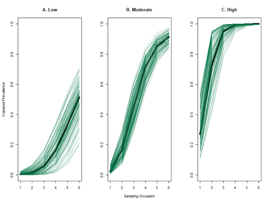
Simulation of copepod prevalence curves for a hypothetical population of juvenile Chinook salmon (Oncorhynchus tshawytscha) for three different year-types (Low, Moderate, High) over five sampling occasions. Green lines are random draws from the curve families for each year-type. The black line represents the curve at median of the uniform distribution for each parameter.
We produced a series of simulated datasets with common characteristics varying only the number of years in the study, the type of copepod infection curves in each year, and the number of fish subsampled during each sampling occasion. For simplicity, all fish in the simulation were released as a single group at the start of the simulated study. The common characteristics included the number of distinct PBT family groups , the total number of juveniles released , the number of primary and secondary sampling occasion, the capture probability during each secondary sampling occasion , and the parameters determing survival. The survival parameters were logit-scaled and included an intercept (, the slope of the time effect (, and the slope of the copepod effect (. These correspond to a baseline survival of 75 percent at and (where is the prevalence of copepod infection in the population), a survival of 95 percent at and , and a survival of 20 percent at and (that is, 100 percent of population infected). Figure 4 depicts the combined effect of both covariates as well as the marginal effect of each (time in blue, copepod prevalence in red) for an example copepod prevalence curve. We simulated 96 datasets for analysis using a multi-year version of the PBT N-mixture model. These datasets consisted of three replicates of each specific combination of number of years, year-types, and subsampling rates. We considered two subsampling rates: 10 fish per sample period and 30 fish per sample period. We simulated datasets covering 2 and 3 years and considered each potential combination of year-types. For example, for the 2-year models the year types consisted of “Low-Low,” “Low-Moderate,” “Low-High,” “Moderate-Moderate,” “Moderate-High,” and “High-High.”
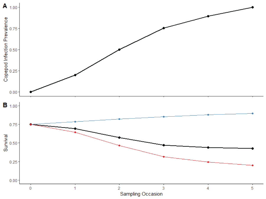
Example survival curves used in the simulation model, (A) example copepod infection prevalence used to generate survival curves in bottom panel, and (B) the red line represents the effect of copepod infection prevalence on survival, ignoring the time effect and the blue line represents the effect of time, ignoring the copepod effect. The black line depicts survival as result of both effects and is the representative survival curve used in the simulation model. On the x-axis, Sampling Occasions occur over time (months since release).
Each simulated dataset was constructed by iteratively stepping through the data generating process implied by the PBT N-mixture model. The simulations began with a release of fish divided among release groups at time . Because we assume that copepod infection rate is zero for the first time step, these fish survive to time with probability equal to logit() = 0.75. Prior to sampling, surviving uninfected fish (all fish at time ) are “infected” with copepods with the probability of infection being determined by the copepod infection curve drawn for that simulation. Surviving fish were then “captured” through removal sampling over sampling occasions with the probability of being captured equal to . Captured fish were then subject to random sampling to be assigned to the subsample group for “histopathology” to determine infection status. For the remaining time periods, the probability of survival from time to was calculated based on the population level infection rate at time () according to the relation logit and the process of “infection,” capture, and subsampling was repeated. If fewer fish were captured than the assigned subsampling rate, then all captured fish were used for simulated histopathological examination.
Each simulated dataset was analyzed using a modified version of the PBT N-mixture model described above. The model was modified to apply to multiple years by looping over likelihoods for all years. Capture probability was also simplified because we ignored the complexities of multiple gear-types and off-shore/on-shore effects for the purposes of simulation. The final modifications accounted for uncertainty in the true copepod infection prevalence because of the subsampling effect and related survival to the latent true infection prevalence. That is for each timestep, we assumed , where is the number of fish subsampled and is the number of these fish with signs of copepod infection. We then estimated survival according to the relation . We evaluated each simulation in terms of Type S and Type M errors (Gelman and Carlin, 2014). Type S errors are errors of the sign of the estimate, if the 90 percent posterior uncertainty interval for and contained both positive and negative values or contained only negative values for and only positive values for then this would be an instance of Type S error. Type M errors are errors of the magnitude of the estimate, which would be the case where the true parameter value was not in 90 percent posterior uncertainty value. In evaluating the model’s ability to detect an effect of both time (predation) and copepod infection, Type S error takes precedence over Type M error. That is, if credible intervals are of the correct sign, but wrong magnitude (Type S error negative, type M error positive) then we can conclude that time and copepods have a positive and negative effect respectively; even if the absolute value of that effect is incorrect, we can use this as a basis for making management decisions. On the other hand, if the credible interval contains the true parameter value but also contains values of the opposite sign, then we cannot conclude there is any effect and thus cannot improve the information on which we base decisions. Because of the limited number of replications (a consequence of limited computational efficiency), our analysis of Type M and Type S error rates are only qualitative.
The results of the simulation study must be interpreted with caution because it makes several assumptions which may not hold in the field. Among these, we assumed that the survival effects would be constant from year to year, which is unlikely to be the case in nature. We also assumed that there was no interaction between time (a surrogate of fish size) and copepod infection which may not hold in nature. Examples of interactions between the two covariates include the following: (1) if larger fish are more likely to die from copepod infection than smaller fish (given equal infection rates); or (2) if larger fish are more likely to be infected but equally likely to die from infection. The true field implementation is also likely to be more complicated than the relatively simple simulation model obtained here; in particular, capture probability was set to be a constant. If it is necessary to account for additional parameters (for example, capture probabilities from different gear types) this may reduce the ability of the model to detect an effect. There is no empirical evidence for the effect of copepod infection prevalence as defined here (that is, infection damage prior to the appearance of adult copepods) and an effect of lesser magnitude is less likely to be detected. Finally, it is unclear whether such a subsampling approach is feasible in a field study; that is, we do not know if gill tissue recovered in the field will be of sufficient quality for histopathological examination.
Results
Re-Analysis of 2018 Lookout Point Data
Re-analysis of the 2018 Lookout Point data was unable to identify separate effects of both time and copepod adult prevalence on survival. Whereas both the “predation only” and “copepod only” models detected a negative effect of the respective covariate, the model with both covariates estimated a negative effect for time that was larger than the effect of the “predation only” model and a positive effect with high uncertainty for the copepod model (fig. 5A). Additionally, the 90 percent posterior uncertainty model for the copepod effect in the combined model overlapped zero which can be interpreted as a non-significant effect. That is, there is some non-negligible probability that the effect of copepods could be either negative or positive. Survival estimates between the three models were similar, with the posterior interval overlapping for all time periods except the third and last (fig. 5B). These results are consistent with what one would expect under multicollinearity; that is, the data are insufficient to estimate separate contributions between the two covariates.
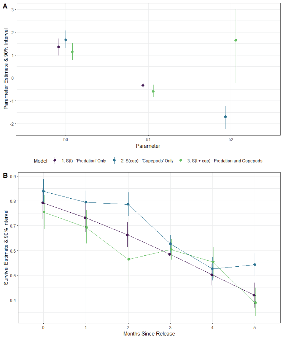
Graphs showing (A) parameter estimates and 90-percent posterior uncertainty intervals for the coefficients of survival (S) of the PBT N-mixture model applied to field data from Lookout Point in 2018. b0 is the intercept, b1 is the slope of time, and b2 is the slope of the copepod effect. The red dashed line is zero; if the posterior interval overlaps the red-dashed line then the model was unable to successfully detect an effect of that covariate, and (B) time period specific estimates of survival for three models. Symbols show the point estimates for survival (S) and whiskers show the 90-percent credible intervals. The x-axis represents time, in months, since release.
Multi-Year Data Simulation with Subsampling
The multiyear data simulation suggests that identifying a signal of the two countervailing covariates will be challenging. Of 96 simulated datasets, only 6 had both 90 percent posterior intervals which contained the true values and did not overlap zero. That is, these simulations had neither Type S nor Type M error. Two of these occurred in simulations of 2-year studies (36 total simulations, fig. 6) and four occurred in simulations of 3-year studies (60 total simulations, fig. 7). All 6 occurred in simulations where the subsample rate was set to 30 fish per sample. All but one occurred in simulations where the year-type combinations included more than one year-type and only one year-type class had more than one replication successfully estimate both parameters (“Low-Low-Moderate”). The models were somewhat better at distinguishing the effect of copepod infection rate alone (18 of 96). When considering only Type S error, 8 out of 96 models got the direction but not magnitude of the effect correct for both covariates, whereas 28 out of 96 models got the direction but not the magnitude correct for the copepod effect alone.
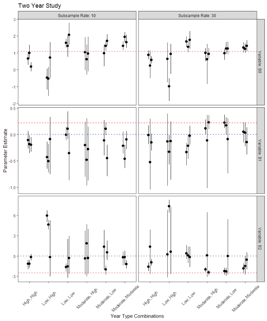
Parameter estimates and 90-percent posterior uncertainty intervals for the coefficients of survival in the simulated 2-year PBT N-mixture model. B0 is the intercept, B1 is the slope of time, and B2 is the slope of the copepod effect. The red dashed line is the true parameter value, and the blue dotted line for the slope terms is zero. For B1, if the posterior interval is entirely above the blue-dotted line and overlaps the red-dashed line then the model was able to successfully detect that effect for that replication of the model. For B2, the interval should be below the blue-dotted line and overlapping the red-dashed.
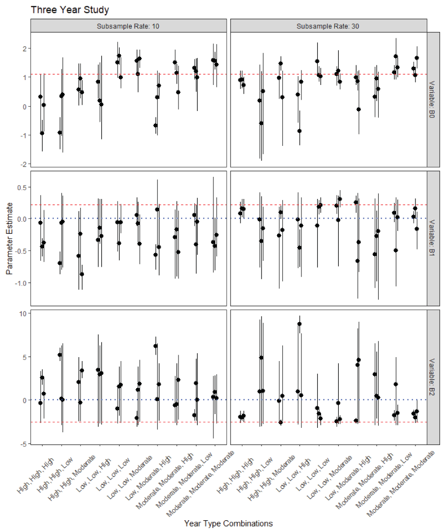
Parameter estimates and 90-percent posterior uncertainty intervals for the coefficients of survival in the simulated 3-year PBT N-mixture model. B0 is the intercept, B1 is the slope of time, and B2 is the slope of the copepod effect. The red dashed line is the true parameter value, and the blue dotted line for the slope terms is zero. For B1, if the posterior interval is entirely above the blue-dotted line and overlaps the red-dashed line then the model was able to successfully detect that effect for that replication of the model. For B2, the interval should be below the blue-dotted line and overlapping the red-dashed.
Discussion
Identifying relations between environmental conditions and ecological processes from observational studies is a challenging endeavor. Environmental conditions often covary (for example temperature and river flow) and ecological process (for example, survival of fish species) are often only imperfectly observed and must be estimated using models paired to rigorous field study designs. Results from this study showed that several limitations exist which prevent the PBT N-mixture model from estimating mortality separately for predation- and copepod-related covariates in Lookout Point Reservoir. These include limitations in recapture probabilities, correlation between covariates of interest, the anticipated duration of a future multi-year field study (2 or 3 years), and critical uncertainties about methods to assess copepod infection and the effect of copepod infection on juvenile salmon survival. Whereas the PBT N-mixture has proven useful for estimating survival and trends in survival when other methods fail, it is important to acknowledge these limitations.
Recapture probabilities during field studies in 2017 and 2018 were very low, ranging from 0.00074 to 0.01303 (Kock and others, 2019a, b). This factor introduces substantial uncertainty into survival estimation. Such low recapture probabilities preclude the effective use of traditional mark-recapture methods (Kock and others, 2019a). Whereas the PBT N-mixture model can obtain survival estimates even with such low recapture probabilities, it may make it impossible to discern small or even moderate effects of covariates on survival using the PBT N-mixture model. The 2017 and 2018 field studies relied on electrofishing, shoreline traps, and gill nets for fish collection and substantial staff time to achieve collection rates observed during the studies. Unless other approaches (for example, trawling) are tested and prove to result in substantial increases in catch, it is unlikely that future field studies will achieve recapture probabilities that allow for improvements in the ability of the survival model to estimate covariate effects on survival probabilities. If opportunities to increase recapture probabilities are indeed limited, then other means of increasing the power of statistical models to detect a trend may need to be implemented. These could include increasing the number of fish released or combining data collected over multiple field seasons.
Correlation between two or more predictor variables (multicollinearity) greatly complicates the ability for any statistical model to obtain reliable estimates of the independent contribution of each predictor to the observed outcome. In the case of copepod infection and predation, both are expected to change monotonically over the course of a field season, which leads to multicollinearity. Absent the ability to experimentally manipulate these two covariates in the field, the only way to realistically reduce the influence of multicollinearity is to collect data over multiple field seasons in the hope that the relation between copepod infection and predation differs between years. We developed the simulation for this study to include 2-year and 3-year scenarios based on the assumption that funding entities would be unwilling to commit to expensive, multi-year studies that extended beyond 3 years. Simulation results showed that four of the six simulated datasets without Type S or Type M errors occurred during the 3-year study period, which illustrate the value of additional years in contributing to modeling success. However, the only successful simulations of multiyear studies occurred when years were drawn from different copepod curve-families. Thus, the ability of a multiyear study to discriminate an effect is likely to be reliant on substantial interannual variation over the course of the study. For example, studies that pair wet, cold years with one or more hot, dry years are more likely to produce different relations between time and copepod infection than a study that included years with similar climatic conditions. The potential value of these additions to the data could be considered along with financial costs associated with additional years of study and the likelihood of conducting a study over a set of years with sufficient interannual variation.
Finally, whereas recent studies have provided new insights into the effects of copepods on the performance and survival of juvenile Chinook salmon, critical uncertainties remain. Several recent studies have assessed copepod effects on juvenile Chinook salmon in field (Beeman and others, 2015; Monzyk and others, 2015b; Murphy and others, 2022) and laboratory (Herron and others, 2018; Murphy and others, 2020a, b; Neal and others, 2021) settings. Results from these studies provided new information by documenting copepod infected Chinook salmon in Willamette Valley reservoirs, describing gill damage caused by copepods, and demonstrating that copepod infection negatively affects juvenile Chinook salmon performance and survival. However, basic questions about copepod effects still exist. For example, Neal and others (2021) showed that juvenile copepods can severely damage gill filaments of juvenile Chinook salmon. However, it’s not clear if this damage leads to direct mortality in the wild. If mortality does occur, the proportion of fish that die, and elapsed time to death are also important unknowns. It is also possible that copepod-induced gill damage affects juvenile Chinook salmon behavior in a manner that increases the likelihood of predation. Finally, it is not clear that gill damage can be assessed in the field for sufficient numbers of captured fish to inform modeling efforts. For survival modeling, these are important critical uncertainties.
References Cited
Beeman, J.W., Hansel, H.C., Hansen, A.C., Evans, S.D., Haner, P.V., Hatton, T.W., Kofoot, E.E., Sprando, J.M., and Smith, C.D., 2014, Behavior and dam passage of juvenile Chinook salmon at Cougar Reservoir and Dam, Oregon, March 2012–February 2013: U.S. Geological Survey Open-File Report 2014–1177, 52 p., accessed on April 25, 2022, at https://pubs.usgs.gov/of/2014/1177/.
Beeman, J.W., Hansen, A.C., and Sprando, J.M., 2015, Observational data on the effects of infection by the copepod Salmincola californiensis on the short- and long-term viability of juvenile Chinook salmon (Oncorhynchus tshawytscha) implanted with telemetry tags: Animal Biotelemetry, v. 3, p. 1–7, accessed April 25, 2022, at https://doi.org/10.1186/s40317-015-0056-5.
Brandt, J.R., Monzyk, F.R., Romer, J.D., and Emig, R., 2016, Status and trends of predator species in Lookout Point Reservoir: Report by the Oregon Department of Fish and Wildlife to the U.S. Army Corps of Engineers, 44 p., accessed on April 25, 2022, at https://odfw.forestry.oregonstate.edu/willamettesalmonidrme/sites/default/files/reservoir-research/status_and_trends_of_predator_species_in_lookout_po int_reservoir-with_npm_rt_-final.pdf.
Gelman, A., and Carlin, J., 2014, Beyond power calculations—Assessing type S (sign) and type M (magnitude) errors: Perspectives on Physiological Science, v. 9, p. 641–651, accessed April 28, 2022, at https://doi.org/10.1177/1745691614551642.
Herron, C.L., Kent, M.L., and Schreck, C.B., 2018, Swimming endurance in juvenile Chinook salmon infected with Salmincola californiensis: Journal of Aquatic Animal Health, v. 30, p. 81–89, accessed April 25, 2022, at https://doi.org/10.1002/aah.10010.
Keefer, M.L., Taylor, G.A., Garletts, D.F., Helms, C.K., Gauthier, G.A., Pierce, T.M., and Caudill, C.C., 2013, High-head dams affect downstream fish passage timing and survival in the Middle Fork Willamette River: River Research and Applications, v. 29, p. 483–492, accessed April 25, 2022, at https://doi.org/10.1002/rra.1613.
Kock, T.J., Perry, R.W., Hansen, G.S., Haner, P.V., Pope, A.C., Plumb, J.M., Cogliati, K.M., and Hansen, A.C., 2019a, Evaluation of Chinook salmon (Oncorhynchus tshawytscha) fry survival in Lookout Point Reservoir, Western Oregon, 2017: U.S. Geological Survey Open-File Report 2019–1011, 42 p., accessed on April 25, 2022, at https://pubs.er.usgs.gov/publication/ofr20191011.
Kock, T.J., Perry, R.W., Hansen, G.S., Haner, P.V., Pope, A.C., Plumb, J.M., Cogliati, K.M., and Hansen, A.C., 2019b, Juvenile Chinook salmon (Oncorhynchus tshawytscha) survival in Lookout Point Reservoir, Oregon, 2018: U.S. Geological Survey Open-File Report 2019–1097, 41 p., accessed on April 25, 2022, at https://doi.org/10.3133/ofr20191097.
Kock, T.J., Perry, R.W., Monzyk, F.R., Pope, A.C., and Plumb, J.M., 2016, Development of a study design and implementation plan to estimate juvenile salmon survival in Lookout Point Reservoir and other reservoirs of the Willamette Project, western Oregon: U.S. Geological Survey Open-File Report 2016–1211, 25 p., accessed on April 25, 2022, at https://doi.org/10.3133/ofr20161211.
Kock, T.J., Beeman, J.W., Hansen, A.C., Hansel, H.C., Hansen, G.S., Hatton, T.W., Kofoot, E.E., Sholtis, M.D., and Sprando, J.M., 2015, Behavior, passage, and downstream migration of juvenile Chinook salmon from Detroit Reservoir to Portland, Oregon, 2014–15: U.S. Geological Survey Open-File Report 2015–1220, 40 p., accessed on April 25, 2022, at https://pubs.er.usgs.gov/publication/ofr20151220.
Lee, S.Y., 2020, Estimation of COVID-19 spread curves integrating global data and borrowing information: PLoS One, v. 15, p. e0236860, accessed April 25, 2022, at https://doi.org/10.1371/journal.pone.0236860.
Monzyk, F.R., Emig, R., Romer, J.D., and Friesen, T.A., 2015a, Life-history characteristics of juvenile spring Chinook salmon rearing in Willamette Valley reservoirs: Report by the Oregon Department of Fish and Wildlife to the U.S. Army Corps of Engineers, 56 p., accessed on April 25, 2022, at https://odfw.forestry.oregonstate.edu/willamettesalmonidrme/sites/default/files/reservoir-research/life-history_characteristics_in_reservoirs_2013-fin al.pdf.
Monzyk, F.R., Friesen, T.A., and Romer, J.D., 2015b, Infection of juvenile salmonids by Salmincola californiensis (Copepoda—Lernaeopodidae) in reservoirs and streams of the Willamette River Basin, Oregon: Transactions of the American Fisheries Society, v. 144, p. 891–902, accessed April 25, 2022, at https://doi.org/10.1080/00028487.2015.1052558.
Muir, W.D., Smith, S.G., Williams, J.G., Hockersmith, E.E., and Skalski, J.R., 2001, Survival estimates for migrant yearling Chinook salmon and steelhead tagged with passive integrated transponders in the lower Snake and lower Columbia Rivers, 1993–1998: North American Journal of Fisheries Management, v. 21, p. 269–282, accessed April 25, 2022, at https://doi.org/10.1577/1548-8675(2001)021<0269:SEFMYC>2.0.CO;2.
Murphy, C.A., Gerth, W., Neal, T., and Arismendi, I., 2022, A low-cost, durable, submersible light trap and customizable LED design for pelagic deployment and capture of fish parasite Salmincola sp. Copepodids: NeoBiota, v. 73, p. 1–17, accessed May 4, 2022, at https://doi.org/10.3897/neobiota.73.76515.
Murphy, C.A., Gerth, W., and Arismendi, I., 2020a, Hatching and survival of the salmon ‘gill maggot’ Salmincola californiensis (Copepoda—Lernaeopodidae) reveals thermal dependence and undocumented naupliar stage: Parisitology, v. 147, p. 1338–1343, accessed April 25, 2022, at https://doi.org/10.1017/S0031182020001109.
Murphy, C.A., Gerth, W., Pauk, K., Konstantinidis, P., and Arismendi, I., 2020b, Hiding in plain sight—Historical fish collections and contemporary parasite research: Bethesday, Maryland, Fisheries, v. 45, p. 263–270, accessed May 4, 2022, at https://doi.org/10.1002/fsh.10411.
Murphy, C.A., Romer, J.D., Stertz, K., Arismendi, I., Emig, R., Monzyk, F., and Johnson, S.L., 2021, Damming salmon fry—Evidence for predation by non-native warmwater fishes in reservoirs: Ecosphere, v. 12, p. e03757, accessed April 25, 2022, at https://esajournals.onlinelibrary.wiley.com/doi/full/10.1002/ecs2.3757.
National Oceanic and Atmospheric Administration, 2008, Endangered Species Act section 7(a)(2) consultation biological opinion and Magnuson-Stevens Fishery Conservation and Management Act essential fish habitat consultation—Consultation on the Willamette River Basin Flood Control Project: National Oceanic and Atmospheric Administration Fisheries Log Number FIWR12000/02117, June 11, 2008, accessed May 10, 2015, at https://www.nwcouncil.org/sites/default/files/willamette_biop_final_part1_july_2008.pdf.
Neal, T., Kent, M.L., Sanders, J., Schreck, C.B., and Peterson, J.T., 2021, Laboratory infection rates and associated mortality of juvenile Chinook salmon (Oncorhynchus tshawytscha) from parasitic copepod (Salmincola californiensis): Journal of Fish Diseases, v. 44, p. 1423–1434, accessed April 25, 2022, at https://doi.org/10.1111/jfd.13450.
Perry, R.W., Skalski, J.R., Brandes, P.L., Sandstrom, P.T., Klimley, P., Ammann, A., and MacFarlane, B., 2010, Estimating survival and migration route probabilities of juvenile Chinook salmon in the Sacramento-San Joaquin River Delta: North American Journal of Fisheries Management, v. 30, p. 142–156, accessed April 25, 2022, at https://doi.org/10.1577/M08-200.1.
Richards, F.J., 1959, A flexible growth function for empirical use: Journal of Experimental Botany, v. 10, p. 290–301, accessed April 25, 2022, at https://doi.org/10.1093/jxb/10.2.290.
Sanders, J., Kent, M.L., Schreck, C.B., Gardner, E., Dew, A., Larson, M., Couch, C.E., and Peterson, J.T., 2021, Spatiotemporal incidence of infection severity of a copepod, S. californiensis, that parasitizes juvenile Chinook salmon in the Willamette River Basin: Draft Annual Report for the U.S. Army Corps of Engineers: Portland, OR, Portland District.
Sard, N.M., O’Malley, K.G., Jacobson, D.P., Hogansen, M.J., Johnson, M.A., and Banks, M.A., 2015, Factors influencing spawner success in a spring Chinook salmon (Oncorhynchus tshawytscha) reintroduction program: Canadian Journal of Fisheries and Aquatic Sciences, v. 72, p. 1390–1397, accessed April 25, 2022, at https://doi.org/10.1139/cjfas-2015-0007.
Skalski, J.R., Smith, S.G., Iwamoto, R.N., Williams, J.G., and Hoffman, A., 1998, Use of passive integrated transponder tags to estimate survival of migrant juvenile salmonids in the Snake and Columbia Rivers: Canadian Journal of Fisheries and Aquatic Sciences, v. 55, p. 1484–1493, accessed April 25, 2022, at https://doi.org/10.1139/f97-323.
Skalski, J.R., Weiland, M.A., Ham, K.D., Ploskey, G.R., McMichael, G.A., Colotelo, A.H., Carlson, T.J., Woodley, C.M., Eppard, M.B., and Hockersmith, E.E., 2016, Status after 5 years of survival compliance testing in the Federal Columbia River Power System (FCRPS): North American Journal of Fisheries Management, v. 36, p. 720–730, accessed April 25, 2022, at https://doi.org/10.1080/02755947.2016.1165775.
For more information about the research in this report, contact
Director, Western Fisheries Research Center
U.S. Geological Survey
6505 NE 65th Street
Seattle, Washington 98115-5016
https://www.usgs.gov/centers/wfrc
Manuscript approved on September 30, 2022
Publishing support provided by the U.S. Geological Survey
Science Publishing Network, Tacoma Publishing Service Center
Disclaimers
Any use of trade, firm, or product names is for descriptive purposes only and does not imply endorsement by the U.S. Government.
Although this information product, for the most part, is in the public domain, it also may contain copyrighted materials as noted in the text. Permission to reproduce copyrighted items must be secured from the copyright owner.
Suggested Citation
Hance, D.J., Kock, T.J., Perry, R.W., and Pope, A.C., 2022, Assessing the efficacy of using a parentage-based tagging survival model to evaluate two sources of mortality for juvenile Chinook salmon (Oncorhynchus tshawytscha) in Lookout Point Reservoir, Oregon: U.S. Geological Survey Open-File Report 2022–1096, 14 p., https://doi.org/10.3133/ofr20221096.
ISSN: 2331-1258 (online)
Study Area
| Publication type | Report |
|---|---|
| Publication Subtype | USGS Numbered Series |
| Title | Assessing the efficacy of using a parentage-based tagging survival model to evaluate two sources of mortality for juvenile Chinook salmon (Oncorhynchus tshawytscha) in Lookout Point Reservoir, Oregon |
| Series title | Open-File Report |
| Series number | 2022-1096 |
| DOI | 10.3133/ofr20221096 |
| Publication Date | November 01, 2022 |
| Year Published | 2022 |
| Language | English |
| Publisher | U.S. Geological Survey |
| Publisher location | Reston, VA |
| Contributing office(s) | Western Fisheries Research Center |
| Description | v, 14 p. |
| Country | United States |
| State | Oregon |
| Other Geospatial | Lookout Point Reservoir |
| Online Only (Y/N) | Y |