

Documenting Arctic Sea Ice Dynamics with Global Fiducials Program Imagery
Links
- Document: Report (37.5 MB pdf) , HTML , XML
- NGMDB Index Page: National Geologic Map Database Index Page (html)
- Download citation as: RIS | Dublin Core
Acknowledgments
Special thanks are due to Harumi Warner, of Parallel Inc., for development of Python scripts and to the late Stan Wilds, also of Parallel Inc., for assistance in figure and table preparation. Early versions of this report were written primarily by Earl M. Wilson. Following his retirement, the scope of the manuscript was expanded, reformatted, and updated by Bruce F. Molnia. The authors wish to thank Florence Fetterer (National Snow and Ice Data Center, University of Colorado) and Ron Kwok (Polar Science Center, Applied Physics Laboratory, University of Washington) for reviewing the manuscript.
Abstract
For more than 25 years, the U.S. Geological Survey (USGS) has used the remote-sensing capabilities of United States National Imagery Systems (USNIS) to obtain high-resolution electro-optical imagery to monitor Earth’s response to global environmental change. A major focus has been monitoring sea ice behavior in the Arctic Ocean and its marginal seas.
In 1997 and 1998, under the direction of the Global Fiducials Program (GFP), USNIS imagery was collected during the Surface Heat Budget of the Arctic Ocean (SHEBA) Project. In 1999, collection of USNIS imagery of six static sea ice sites in the Arctic Ocean and its marginal seas began, and the imagery was archived in the USGS-hosted Global Fiducials Library (GFL). The static sites were imaged through 2014, creating time series of geographically referenced images which scientists have used to study seasonal changes in Arctic ice over the same locations for extended time periods.
In early 2009, the Central Intelligence Agency’s MEDEA Program requested that the USGS use USNIS imagery to track movements of sea ice floes during an entire Arctic summer (April through September). The goal was to improve researchers’ understanding of seasonal changes in Arctic sea ice. In order to track and repeatedly capture imagery of the same ice as it drifted across the Arctic Ocean, the USGS developed a methodology and a series of protocols to use data from telemetering drift buoys deployed at locations across the Arctic Ocean by the International Arctic Buoy Programme (IABP) to track the drift of targeted ice masses for periods that exceeded a year. Resulting time series of sea ice imagery, captured while monitoring 38 individual buoys, were archived in the GFL.
In 2013 and 2014, in support of the Seasonal Ice Zone Reconnaissance Surveys (SIZRS) Program led by the University of Washington, Seattle, Washington, the USGS requested the collection of USNIS imagery of selected sites in the Beaufort and Chukchi Seas located at every degree of latitude between 70° and 80° N. along a north-south transect. This was done to track and understand the interplay among the ice, atmosphere, and ocean and what it contributes to the rapid decline in summer ice extent that has occurred in recent years.
Under the auspices of the GFP, thousands of sea ice images have been collected. Many of those that pass a quality and cloud-cover screening are archived in the GFL. Of these, more than 1,750 sea ice images have been publicly released, following an editing and processing procedure that produces high-resolution degraded images, known as “literal imagery-derived products” or LIDPs. These LIDPs have been approved for free, unrestricted public distribution and scientific analysis. The LIDPs can be downloaded from the USGS Global Fiducials Library Data Access Portal (USGS GFLDAP) at https://www.usgs.gov/global-fiducials-library-data-access-portal. In addition, nonliteral imagery-derived products (nonliteral IDPs), such as metadata, maps, charts, and graphs, have also been released.
Introduction
Arctic sea ice is a key component of the polar climate system. Typically, it is monitored remotely from space, from the air, and by direct observations from ships and floating ice islands. Physical parameters that are monitored include temporal and geographic extent, ice area, ice age, and ice thickness. Additionally, the movement of sea ice in response to wind and ocean currents is documented through the collection and analysis of imagery time series.
Since late 1978, scientists have systematically monitored the extent of Arctic sea ice cover from space by using passive microwave satellite imagery collected by the U.S. Defense Meteorological Satellite Program (DMSP) instruments (Peng and others, 2013). Sea ice and other Earth surface features emit measurable low-level electromagnetic energy in the microwave range of the spectrum. The DMSP sensors detect this naturally emitted passive microwave radiation. Compared to clouds and ocean water, sea ice emits significantly more microwave radiation. Consequently, the passive microwave energy produced by sea ice, which penetrates clouds, is used to detect sea ice, both day and night, regardless of cloud cover.
According to the National Snow and Ice Data Center’s “Cryosphere Glossary” (NSIDC, 2023), ice extent is the “total area covered by some amount of ice, including open water between ice floes.” Ice extent is typically reported in square kilometers. A typical threshold between “ice-covered” or “not ice-covered” is 15 percent.
The 15-percent minimum cutoff is used to define the ice edge because it provides the most consistent agreement between satellite and ground observations (NSIDC, 2022b). The sea ice area, typically measured in millions of square kilometers (106 km2), is the part of the sea ice extent that is covered by ice at any point in time. Maximum sea ice coverage usually occurs in March, and minimum sea ice coverage occurs in September before colder weather begins new ice formation.
U.S. agencies that monitor the extent of Arctic sea ice coverage are the National Snow and Ice Data Center (NSIDC), the National Aeronautics and Space Administration (NASA), and the U.S. National Ice Center (NIC). The NIC is a partnership among the U.S. Navy, the National Oceanic and Atmospheric Administration, and the U.S. Coast Guard.
Space-based monitoring of Arctic sea ice began with the launch of NASA’s Scanning Multichannel Microwave Radiometer (SMMR) on October 25, 1978. Consequently, 1979 was the first full year of sea ice satellite observations. During the more than 43 years of satellite monitoring of Arctic sea ice, there have been vast decreases in both the maximum and minimum extents of ice coverage (fig. 1). The absolute minimum Arctic sea ice extent recorded was 3.4×10⁶ km2 in September 2012 (NSIDC, 2022a). The NSIDC’s “Charctic Interactive Sea Ice Graph” (NSIDC, 2022a) depicts ice extents of 3.404×10⁶ km2 on September 15, 2012; 3.389×10⁶ km2 on September 16, 2012; 3.387×10⁶ km2 on September 17, 2012; and 3.418×10⁶ km2 on September 18, 2012. A 2012 NSIDC publication had originally identified September 16 as being the all-time minimum, with an extent of 3.418×10⁶ km2 (NSIDC, 2012).
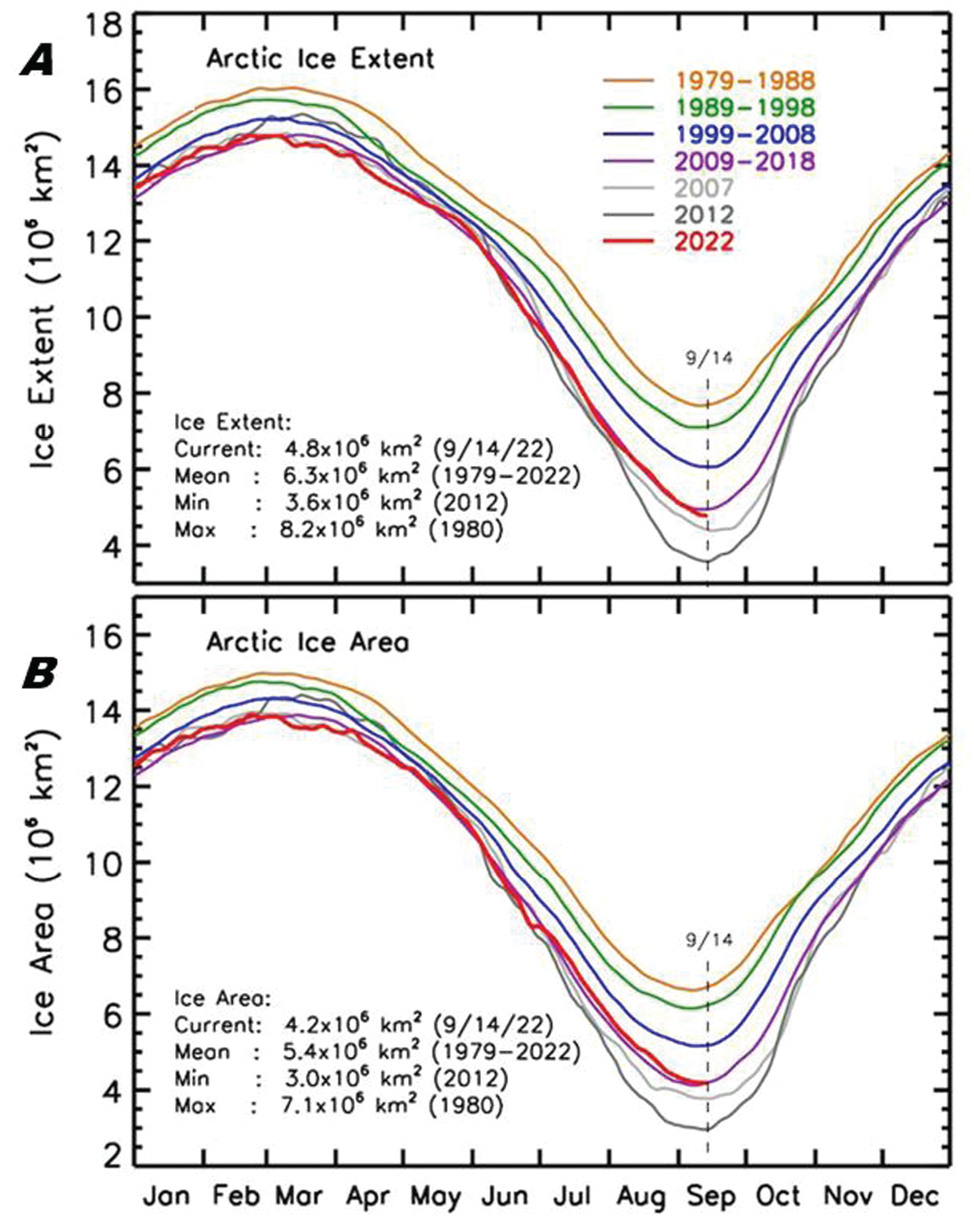
Graphs, updated through September 14, 2022, showing data for (A) Arctic sea ice extent and (B) Arctic sea ice area. The data include 10-year averages from 1979 through 2018 (1979–1988, 1989–1998, 1999–2008, and 2009–2018) and yearly averages for 2007, 2012, and 2022 of the daily sea ice extent and daily sea ice area. Tables in parts A and B list current, mean, minimum, and maximum values for ice extent and ice area, respectively, in millions of square kilometers (106 km2). The sea ice extent on September 14, 2022, was 4.8×10⁶ km2, while the area was 4.2×10⁶ km2. The figure is from Comiso and others (2022, fig. 1).
Since 2012, the annual minimum Arctic sea ice extent has been significantly less than the 30-year average baseline. This 30-year record, which is based on the average ice extent for the period from 1981 to 2010, is frequently used because it provides a consistent sea ice extent baseline for year-to-year comparisons. According to the National Centers for Environmental Information (NCEI, 2021) of the National Oceanic and Atmospheric Administration, 30 years is considered a standard baseline period for weather and climate. Beginning in 1978, the more than 43-year-long satellite record of ice observations is long enough to provide a space-based observational baseline period as well (Meier and others, 2017; NSIDC, 2022a).
For example, based on satellite observations (NSIDC, 2022a), Arctic sea ice daily minimum extent decreased from 7.6×10⁶ km2 on September 13, 1980, to 4.1×10⁶ km2 on September 18, 2007, and then to 3.4×10⁶ km2 on September 17, 2012. Since then, the annual minimum has fluctuated between 5.1×10⁶ km2 on September 13, 2013, and 3.8×10⁶ km2 on September 18, 2020. The 2020 minimum sea ice extent was the second lowest extent measured since modern record keeping began in 1978. The extents in 2007 and 2016 are tied for the third lowest Arctic sea ice extent at 4.1×10⁶ km2 (NSIDC, 2022a). The 2022 minimum (4.7×10⁶ km2 on September 18) is tied for tenth lowest with 2017 and 2018. To put this area and loss into perspective, the size of the conterminous United States is about 8.1×10⁶ km2. Figure 2 depicts the monthly extent of Arctic sea ice in September 1980, 2012, and 2022.
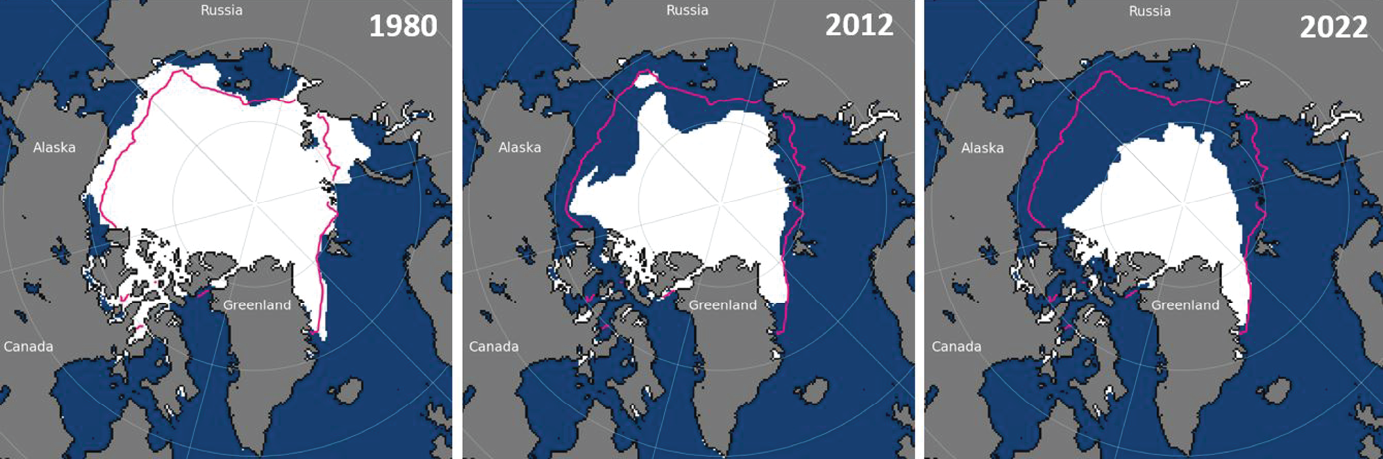
Maps depicting the monthly extent of Arctic sea ice in September 1980, 2012, and 2022. In the Arctic, September is typically the month with the minimum sea ice extent. The total monthly ice extent in September 1980 was 7.7×10⁶ square kilometers (km2); in September 2012, it was 3.6×10⁶ km2; and in September 2022, it was 4.9×10⁶ km2. The three maps show the expanse covered by ice at greater than 15-percent monthly mean concentration. The 2012 extent is the smallest monthly extent ever recorded. The magenta line shows the 1981 to 2010 median sea ice extent for the month of September. Ice extent is based on passive microwave data collected by the U.S. Defense Meteorological Satellite Program (DMSP) F-18 Special Sensor Microwave Imager/Sounder (SSMIS). National Snow and Ice Data Center (NSIDC) maps available from https://nsidc.org/data/masie were modified by the U.S. Geological Survey National Civil Applications Center in 2022 to produce the image.
This report describes the Global Fiducials Program (GFP) and how Global Fiducials imagery has been used to document Arctic sea ice dynamics. The origins and history of the GFP are described and examples are presented depicting how the GFP’s imagery products are uniquely used to document complex sea ice behavior at spatial resolutions previously not publicly available.
Global Fiducials Program and Library
Through the Global Fiducials Program (GFP), the U.S. Geological Survey (USGS) is helping the global science community to study rapidly changing Arctic sea ice behavior by providing free and unrestricted imagery time series of both moving ice containing drift buoys and static sites. The time series document annual and inter-annual variability. The imagery is available at a Global Fiducials Library (GFL) website, the Global Fiducials Library Data Access Portal (USGS GFLDAP) at https://www.usgs.gov/global-fiducials-library-data-access-portal, which is described below.
The GFP was created in the mid-1990s by the Central Intelligence Agency (CIA) through its MEDEA Program in conjunction with a Government Applications Task Force made up of 13 other U.S. Federal agencies, including the USGS (Baker and Zall, 2020). The term “MEDEA” is not an acronym. Rather, it was chosen to complement the name of another U.S. Government advisory group, “JASON,” which comes from the Greek myth related to Jason, Medea, and the Argonauts (Baker and Zall, 2020).
The agencies recognized that exploring the effects of global environmental change required earth science data that could be derived from extremely high resolution United States National Imagery Systems (USNIS) imagery. Such imagery could be used for systematic monitoring of dynamic and environmentally critical areas of the Earth in five major disciplines, which are described at the GFLDAP: ocean processes, land use/land cover, atmospheric processes, ice and snow dynamics, and geologic processes. The study of sea ice is a subset of both the ocean processes discipline and the ice and snow dynamics discipline.
Initially, MEDEA’s data acquisitions were based on input from a group of about 60 U.S. academic scientists who were selected by MEDEA Program managers and who obtained high-level security clearances. Beginning in 1997, Federal agency scientists were also able to nominate new locations for data acquisition.
Individual data-acquisition locations were referred to as “fiducial sites” or “fiducial points.” Each serves as a benchmark for long-term, ongoing monitoring of global environmental change (Baker and Zall, 2020, p. 23).
Following its inception, MEDEA’s GFP identified about 500 worldwide fiducial sites (Dozier, 1997), 6 of which were focused on Arctic sea ice. Collection of USNIS electro-optical images from the sites began in the mid-1990s, with thousands of images being collected (Molnia and others, 2018; Baker and Zall, 2020, p. 23). Many images were not usable because of clouds and haze. To date, most of the collected images remain classified and have not as yet been released to the public.
MEDEA’s Global Fiducials Program existed during 1993–2000 and from 2008 to May 2015, when it was abolished by the CIA. The USGS-led Civil Applications Committee (CAC) directed the GFP from 2000 to 2008 and twice joined with MEDEA to co-lead the program (1997–2000 and 2008–2015). Since 2015, the CAC’s Global Fiducials Working Group (GFWG) has solely led the GFP.
In 1997, the CAC established the Global Fiducials Library (GFL) to serve as a centralized archive for GFP imagery and to provide a mechanism for searching and accessing these data. The “About” page of the USGS GFLDAP site (U.S. Geological Survey, 2022) describes the GFL as follows: “The Global Fiducials Library (GFL) is a long-term archive of images from U.S. National Imagery Systems which represents a long-term periodic record for selected scientifically important sites. The GFL was created to be the collection, archive and data management component of the Global Fiducials Program (GFP).” The “long-term periodic record” consists of imagery time series (that is, sets of images taken sequentially of the same location) from the GFP that document natural hazards and disasters, global change, land resources issues, ecosystem dynamics, and many other types of Earth surface processes. The GFL contains imagery of domestic GFP sites, international GFP sites, Antarctic sites, and Arctic sea ice sites.
Since 2015, the GFWG has solely managed Global Fiducials activities, including the identification of new fiducial sites. Like MEDEA’s fiducial points, a fiducial site is a geographic location that is used as a benchmark for the long-term monitoring of processes, both natural and anthropogenic, associated with the causes and effects of global environmental change. Fiducials are marks or points of reference applied to images to present a fixed standard of reference; in the GFP, they refer to the identification of a place on Earth’s surface. The GFP maintains long-term data records for specific places on Earth’s surface, and the records are made available for scientific investigations. Fiducial sites are associated with Earth processes and environmentally sensitive areas that are being monitored so that scientists can better understand and model the dynamic systems and changes that are occurring. The sites are located around the globe.
According to a report by the U.S. Joint Chiefs of Staff (2017, p. G-9), an imagery-derived product (IDP) is “[a]ny representation made from US classified satellite imagery that is not a direct copy of the original image itself.” An IDP may be analog or digital. A literal IDP is an image-like product that is not a direct copy of the original image, whereas a nonliteral IDP is (1) a graphic product such as a map, a line drawing, a chart, or a graph or (2) metadata or other statistical data derived from imagery. Literal IDPs (LIDPs) have had their pixels digitally manipulated so that the pixels’ original characteristics are irreversibly changed while the appearance of the image remains unchanged. This manipulation is done to prevent adversaries from determining the capabilities of the sensors that collected the original image.
To date, more than 4,400 LIDPs, produced from USNIS images collected in support of the GFP, have been made available for unrestricted public distribution and scientific analysis at a resolution of about a meter. They are available from the USGS GFLDAP at https://www.usgs.gov/global-fiducials-library-data-access-portal. Of these LIDPs, 1,751 are sea ice images collected between 1999 and 2014. Many are accompanied by nonliteral IDPs. Examples of these IDPs appear in later sections of this report.
The CAC represents Federal civil agency interests and requirements in the use of Global Fiducials imagery (Molnia and others, 2012). The CAC facilitates the appropriate Federal civil uses of overhead remote sensing technologies and data collected by military and intelligence agencies and commercial sources. A primary function is ensuring that the personal privacy and civil rights of U.S. persons are not violated by the use of GFP imagery. The CAC is operated and staffed by the USGS on behalf of the U.S. Department of the Interior and its interagency partners (Opstal and Rogers, 2022).
The USGS GFLDAP provides unrestricted access to GFP imagery from more than 150 fiducial sites. Users may search the web portal for existing imagery and preview that imagery and its associated metadata. The USGS GFLDAP web portal (fig. 3) has a fiducial site location map and a brief description about each site. Fiducials imagery is available to preview through an imagery gallery, the Global Fiducials Library Image Gallery website, which is a part of the USGS long-term archive at https://gfl.usgs.gov/imagegallery/?PTAGNAME=ArcticBuoys&img:2573:208.
Screen capture of the main part of the Global Fiducials Library Data Access Portal web page. This is the gateway to Arctic sea ice imagery hosted by the U.S. Geological Survey. The imagery can be downloaded at https://www.usgs.gov/global-fiducials-library-data-access-portal.
Images collected over land are orthorectified to provide terrain-corrected, accurately positioned imagery. This is not done for sea ice images. Images of Arctic buoys and static sea ice sites are orthocorrected to a constant elevation because the sites are at sea level. Arctic sea ice buoy LIDPs have a spatial resolution of 1.3 meters (m). Metadata are also made available for all GFL sea ice imagery products, including Sun elevation and Sun azimuth for the Arctic datasets. All other GFL sites, including the static sea ice sites, have a spatial resolution of 1.0 m.
Studies of four types of GFP Arctic sea ice sites have produced imagery that is in the GFL. Descriptions and images from the four types of sites are listed below:
-
• Images collected during the 1997–1998 Surface Heat Budget of the Arctic Ocean (SHEBA) Project;
-
• Images collected from six static sea ice sites located throughout the Arctic Ocean;
-
• Images collected of sea ice containing 38 drift buoys, many of which were monitored for months; and
-
• Images collected in cooperation with the U.S. Office of Naval Research (ONR) of the Seasonal Ice Zone (SIZ) Region Sites and Marginal Ice Zone (MIZ) Sites.
Why Study Sea Ice Processes?
The extent of Arctic sea ice influences Earth’s climate and albedo. Large areas of ice and snow reflect much of the Sun’s energy back into space, helping to cool the Earth. Darker ocean water or substantial sea ice areas covered with melt ponds (fig. 4A, B) absorb the Sun’s energy, which increases ocean water temperature or accelerates sea ice melting. The more open water that is exposed, the more energy that is absorbed by the ocean. The increase in temperature significantly affects the survival of the sea ice cover during summer. Understanding the mechanisms and triggers of melt pond formation processes becomes critical for choosing data to use in modeling climate changes and the effects of melt ponds on Arctic sea ice extent. Storms and wind-driven waves also play a role in the Arctic sea ice breakup and melting.
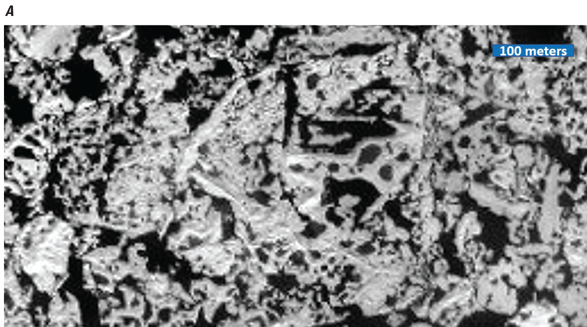
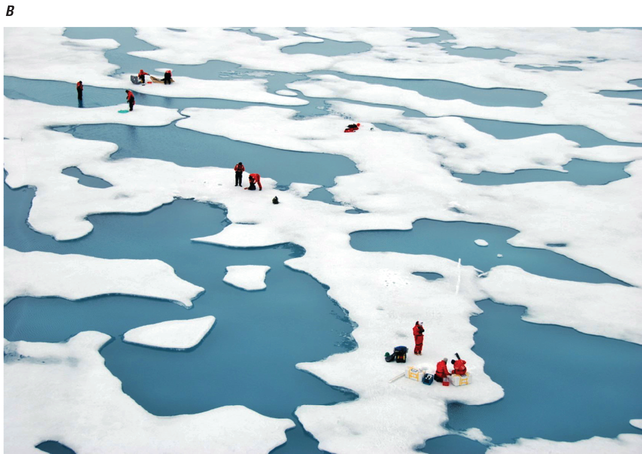
Two views of Arctic sea ice melt ponds. A. Image of sea ice at the Beaufort Sea site in August 2001. More than 40 percent of the image consists of melt ponds located on the surface of densely packed ice floes. The largest melt ponds present are slightly larger than 100 meters in length. The larger ponds form by the coalescing of adjacent ponds. The smallest that are visible are less than 5 meters in maximum dimension. The scale bar in the top right represents 100 meters. The site location is shown in figure 7. This literal imagery-derived product (LIDP) was derived from a U.S. National Imagery Systems electro-optical satellite image. The unannotated image is from the Global Fiducials Library Data Access Portal (https://www.usgs.gov/global-fiducials-library-data-access-portal). B. Photograph of nine scientists conducting a variety of sea ice and melt ponds investigations during an international sea ice research project in 2020 in the Arctic Ocean. Photograph by Melinda Webster, National Aeronautics and Space Administration, Goddard Space Flight Center, Greenbelt, Maryland; used with permission.
In general terms, the extent of sea ice in the Arctic increases in size during the fall and winter months (October through March) when little or no solar radiation reaches the ocean’s surface. This lack of solar radiation permits new first-year ice to form and thicken and, in some locations, to mix with existing ice. During the spring and summer months, the thickness and extent of the sea ice begin to decrease from melting as solar radiation reaching the ocean’s surface increases. If the sea ice does not thicken enough over the winter, it may completely melt away during summer. If the ice grows thick enough during the winter, it will experience thinning during the summer, but it may not completely melt away. In this scenario, the ice will remain until the following winter, when it will again grow and thicken. The ice formed during more than one winter is classified as multiyear ice. During winter, snow may accumulate on the surface of sea ice.
During spring and summer, snow remaining on top of the ice melts, and the resulting meltwater and additional water from melting sea ice accumulate in cracks and depressions on the sea ice surface, forming melt ponds. These melt ponds absorb more heat from the Sun’s radiation compared to the surrounding ice and snow, which typically reflects the sunlight. As the water in the melt ponds warms, the ponds become larger in surface area and deepen, melting into the underlying ice. As the melt ponds become deeper, they can melt through the entire thickness of the sea ice. Channels may form that connect melt ponds and drain meltwater from one melt pond to another.
Imagery in the GFL is of high enough resolution to allow mapping of melt ponds to get estimates of how much of the sea ice, on average, is covered by the darker-than-ice ponds. A melt pond dataset, compiled by Fetterer and others (2008), was based on GFL imagery from the GFL Arctic static ice sites.
Arctic Sea Ice Imagery Available From the Global Fiducials Library
On June 1, 2022, the USGS GFLDAP website displayed 1,751 Arctic sea ice images, collected between 1999 and 2014, that were available for free download. These images represent a subset of the more than 3,138 sea ice images that GFP records indicate were collected during that period, exclusive of SHEBA imagery. The images collection includes the following: 844 images collected from the six static sites, 1,734 images collected of sea ice containing drift buoys, and about 520 images collected of Marginal Ice Zone, Ice Edge, and Seasonal Ice Zone Region sites. The GFP plans for all sea ice imagery collected since 2014 to be added to the GFL website once LIDPs are produced and public release approval is received.
Imagery From the Surface Heat Budget of the Arctic Ocean (SHEBA) Project
The first Arctic sea ice studies began in 1893, when the Norwegian ship Fram, under the command of Fridtjof Nansen, was frozen into the Arctic Ocean as part of an attempt to reach the geographical North Pole (Nansen, 1897). This first systematic effort to monitor Arctic sea ice resulted in significant information about Arctic sea ice dynamics. Seventy-nine years later, the Arctic Ice Dynamics Joint Experiment (AIDJEX) was conducted. According to the NSIDC (2022c), the AIDJEX program was the first major sea ice experiment constructed specifically to answer emerging questions about sea ice movement and changes in the western Arctic Ocean in response to ocean and atmosphere forcing. Initial field deployment in 1972 was followed by expanded field activities in 1975 and 1976. This exceptional study was accomplished without a systematic space-based or aerial high-resolution imagery collection component or capability.
In 1997, 104 years after the Fram expedition, the Surface Heat Budget of the Arctic Ocean (SHEBA) Project began; it was funded by the National Science Foundation (NSF) of the United States (National Science Foundation, 1998). The Canadian icebreaker Des Groseilliers was purposely frozen into sea ice of the Beaufort Sea. The field component of the SHEBA Project lasted for 404 days, from August 25, 1997, to October 3, 1998, with the icebreaker serving as both an experiment platform and a base for scientific researchers. Scientists from across the globe were able to reside on the ship, perform experiments, and conduct field excursions to study and observe sea ice dynamics with the goal of gaining a better understanding of global climate change (Uttal and others, 2002).
Although all participants refer to the activity as “SHEBA,” multiple titles are used when the project name is fully spelled out. The NSF (National Science Foundation, 1998, 2000), which funded the experiment, referred to it as the “Surface Heat Budget of the Arctic Ocean” Project. The National Center for Atmospheric Research (NCAR; undated) also referred to it as the “Surface Heat Budget of the Arctic Ocean” Project, whereas the NSIDC, which cohosts the data, referred to it as the “Surface Heat Balance of the Arctic” Experiment (Fetterer and Untersteiner, 2000). The format used in this report, “Surface Heat Budget of the Arctic Ocean” Project, follows that used by the NSF.
The GFP’s monitoring of sea ice by using high-resolution USNIS satellite imagery began in September 1997. More than 100 USNIS high-resolution images were acquired of the ship and the ice adjacent to it as the ship drifted across the Beaufort Sea. When degraded and released, this GFP imagery was the only publicly available imagery with high enough resolution to document the complex changes that occurred in the sea ice during the period of observation. The resolutions of images from Landsat (15–30 m resolution), commercial satellites collecting electro-optical images (typically 3–5 m resolution), and similar Canadian and European satellites (such as RADARSAT) that were operational at the time of the SHEBA Project were too low to display the small and subtle changes that occurred on the sea ice surface. Median melt pond diameters observed during the SHEBA Project were about 4 m. The SHEBA Project provided the first high-resolution imagery to monitor the behavior of the same ensemble of Arctic sea ice for a significant period of time.
The Des Groseilliers transmitted the latitude and longitude of its changing position as it drifted (fig. 5). The hourly receipt of the ship’s coordinates permitted the USGS to anticipate future ship locations and to schedule time-sensitive new collections designed to reimage the large area (about 15×40 km) of the same sea ice that surrounded the drifting ship. Although most imagery showed significant cloud cover, 57 generally cloud free, optical-band reconnaissance images were reprocessed, and LIDPs were approved for public release by the National Imagery and Mapping Agency (now the National Geospatial-Intelligence Agency) at the request of the NSF. One of these images is presented in figure 6A. Figure 6B depicts the area outlined in red on figure 6A and shows the icebreaker. This publicly released imagery is housed in the GFL, and the LIDPs are available from the NSIDC (Fetterer and Untersteiner, 1998, 2000).
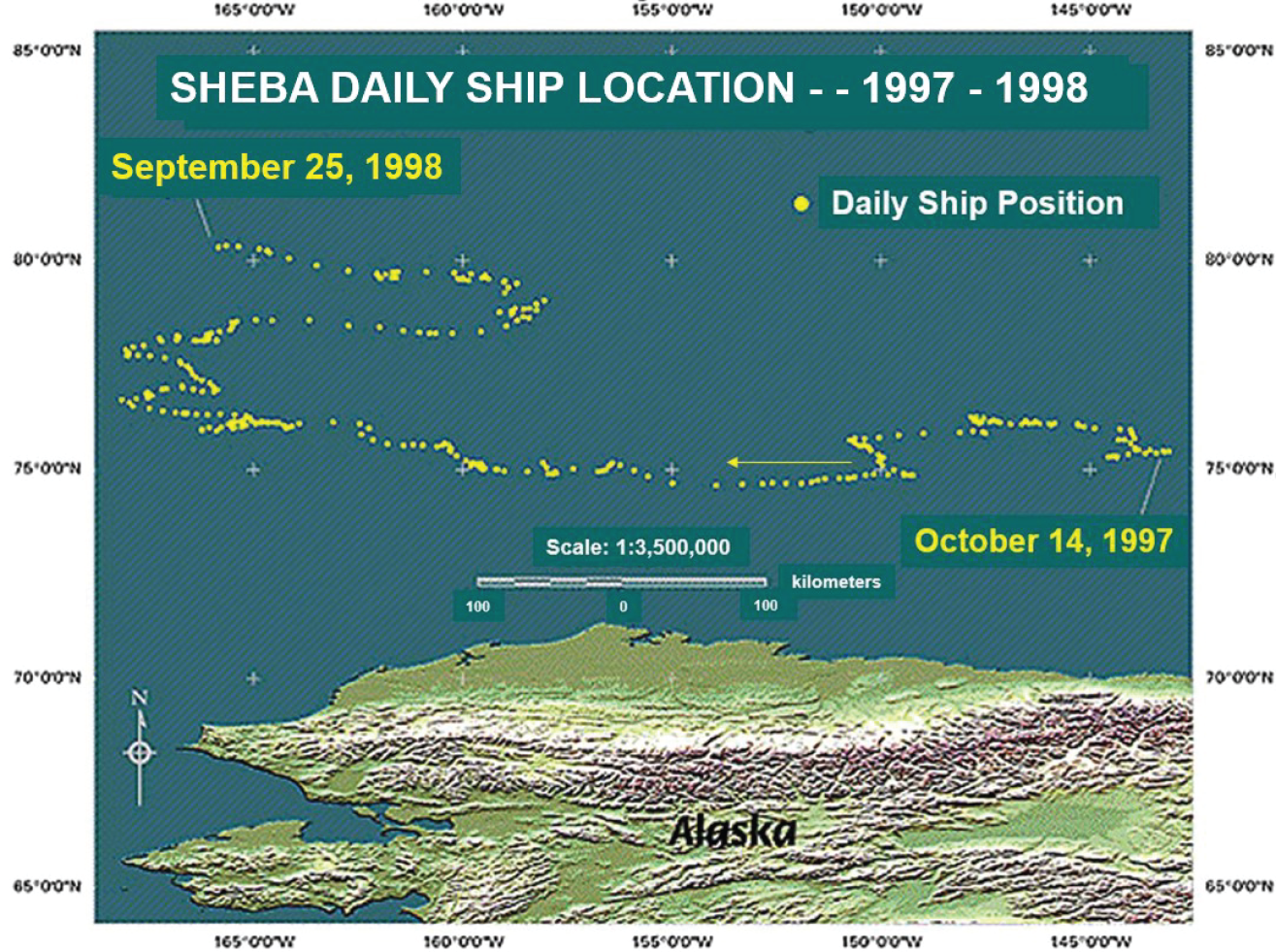
Track map showing the positions of the Canadian icebreaker Des Groseilliers as it drifted westwardly across the Beaufort Sea from October 14, 1997, to September 25, 1998, while embedded in sea ice. Scientists on the icebreaker collected data during the Surface Heat Budget of the Arctic Ocean (SHEBA) Project. The map was produced by the U.S. Geological Survey National Civil Applications Center in 2015.
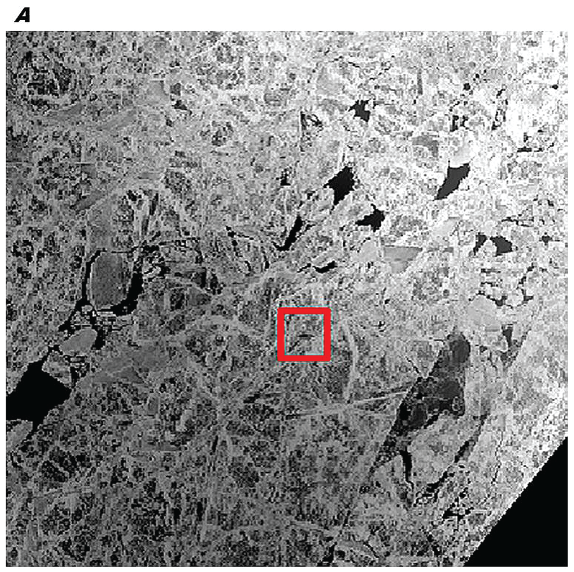
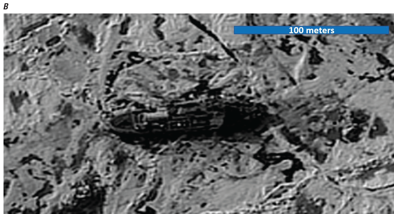
Images of the area where the Canadian icebreaker Des Groseilliers was frozen into the Beaufort Sea icepack in June 1998 during the Surface Heat Budget of the Arctic Ocean (SHEBA) Project. These literal imagery-derived products (LIDPs) were derived from a U.S. National Imagery Systems electro-optical satellite image. A, Image from June 1998 showing the icebreaker (within red rectangle), frozen into the Beaufort Sea icepack. The imaged area is about 7×7 kilometers. B, An enlargement of part of the image shown in part A, providing a closer view of the ship and its surrounding ice. The imaged area in part B, the area within the red rectangle in part A, is about 395×330 meters. The scale bar in the top right represents 100 meters. Many melt ponds (dark areas) are visible on the snow-covered ice surface. The unannotated images are from the Global Fiducials Library Data Access Portal (https://www.usgs.gov/global-fiducials-library-data-access-portal).
Imagery From Six Static Sea Ice Sites in the Arctic Ocean Monitored by the Global Fiducials Program
Following the successful imaging done during the SHEBA Project, in 1999, the GFP began to systematically monitor other Arctic sea ice by using imagery from the USNIS. Initially, six static locations were selected in order to better understand sea ice dynamics, distribution, age, melt history, and annual variability. The sites were “static” in that a finite location (fiducial point) was imaged and whatever ice, if any, that was present was documented. The static sea ice sites (fig. 7) were selected so that the quantity, age, and condition of sea ice could be repeatedly monitored at these unique locations. Four sites had collections over 15-year periods, while two were imaged for 10 years. The publicly released LIDPs have a spatial resolution of about 1.3 m and depict areas that are 2×2 km to 6×6 km in size.
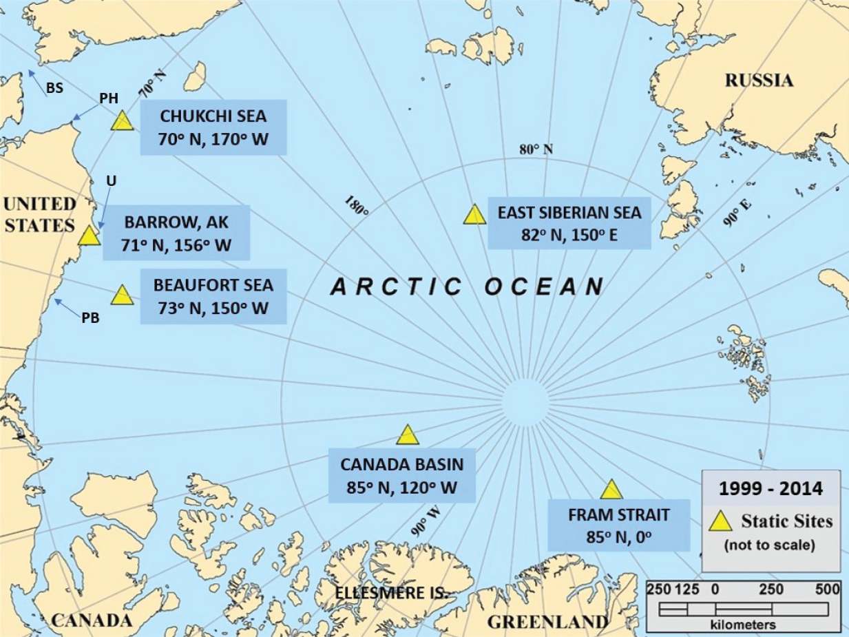
Map of the Arctic Ocean showing the locations and latitude and longitude of the six static sea ice sites monitored by the Global Fiducials Program. Terms: AK, Alaska; BS, Bering Strait; E, east; N, north; PB, Prudhoe Bay; PH, Point Hope; U, Utqiagvik; and W, west. The map was produced by the U.S. Geological Survey National Civil Applications Center in 2015.
The static sea ice sites in the Arctic Ocean (presented from west to east) are described below, and the latitude and longitude are given for each site. The descriptions of the static sites are derived from unpublished MEDEA and CAC documents produced during the GFP’s site selection process.
Chukchi Sea site (lat 70° N., long 170° W.)—The Chukchi Sea site is located about 225 km northwest of Point Hope, Alaska, and about 515 km south-southwest of the city of Utqiagvik (formerly Barrow), Alaska. Historically, the area containing the Chukchi Sea site was near the boundary between older multiyear ice and thinner first-year ice that tended to melt away every summer. Examination of satellite imagery and NSIDC-hosted data by author Molnia has shown that the age and extent of sea ice in this region have significantly declined since the late 1970s. At this site, 80 images were collected between 2005 and 2014.
Barrow, Alaska, site (lat 71° N., long 156° W.)—The Barrow, Alaska, site includes the part of Alaska’s North Slope Borough containing the city of Utqiagvik (formerly Barrow) and extends about 5 km from the shore over the adjacent continental shelf. It is in a location where sea ice forms along the western Alaska coast in winter and generally melts or breaks away by mid-July. Changes in the timing of coastal sea ice breakup and the location of offshore sea ice have significant local ecological, biological, and human effects. The image time series collected at this site portrays changes in the timing of coastal sea ice breakup and provides information on the properties of smaller areas of ice. Figure 8 depicts the variation that occurred in two consecutive years, comparing images collected a year apart in July 2006 and July 2007. At this site, 97 images were collected between 2005 and 2014.
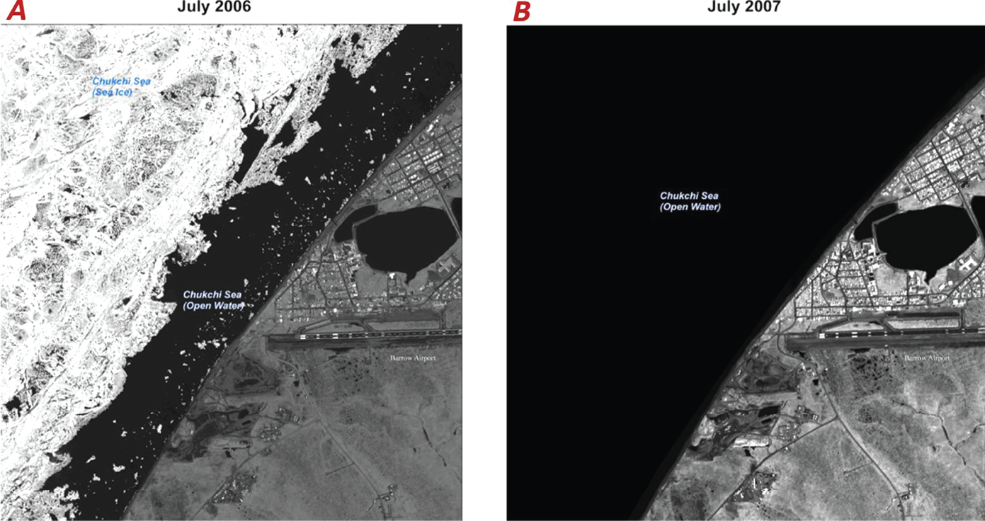
Annotated images of the Barrow, Alaska, site in (A) July 2006 and (B) July 2007. The site was selected to observe annual variability in the formation and breakup of nearshore sea ice. This pair of July images shows the significant difference in ice extent in two consecutive years. In July 2006, the edge of the ice pack was less than a kilometer from shore, whereas in July 2007, the edge of the ice pack was many kilometers offshore, well beyond the limits of the area imaged. The site location is shown in figure 7. Each image depicts an area of about 4.4 km (east–west) by 5.2 km (north–south). The literal imagery-derived products (LIDPs) were derived from U.S. National Imagery Systems electro-optical satellite images. The unannotated images are from the Global Fiducials Library Data Access Portal (https://www.usgs.gov/global-fiducials-library-data-access-portal).
Beaufort Sea site (lat 73° N., long 150° W.)—The Beaufort Sea site is located about 165 km north-northwest of Prudhoe Bay, Alaska. This region has been the site of many field studies since the International Geophysical Year (1957–1958). The site was typically near the edge of the ice pack, but annual ice conditions vary, as is shown by the two images in figure 9. In the August 2001 image, more than 75 percent of the field of view is ice covered. In the August 2007 image, more than 75 percent of the area is ice free. At this site, 163 images were collected between 1999 and 2014.
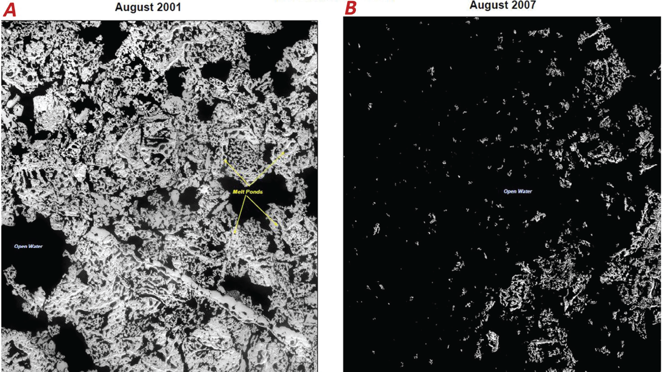
Annotated images of the Beaufort Sea site in (A) August 2001 and (B) August 2007. The site was selected to observe how Arctic sea ice changes during the period of Arctic daylight. This pair of August images shows that significant interannual variability existed between 2001 and 2007. Note the abundant ice with melt ponds on the 2001 image and the much smaller amount of sea ice on the 2007 image. When imaged in 2007, the site was located just south of the southern edge of the ice pack. The site location is shown in figure 7. Each image depicts an area of about 0.9 kilometer (east–west) by 1.0 kilometer (north–south). These literal imagery-derived products (LIDPs) were derived from U.S. National Imagery Systems electro-optical satellite images. The unannotated images are from the Global Fiducials Library Data Access Portal (https://www.usgs.gov/global-fiducials-library-data-access-portal).
Canada Basin site (lat 85° N., long 120° W.)—The Canada Basin site is located about 1,725 km north-northeast of Prudhoe Bay, Alaska, and about 500 km from the closest land on the coast of Ellesmere Island. The Canada Basin site typically has the oldest and thickest ice with the longest residence time in the Arctic Ocean. The GFP Arctic sea ice time series is one of the most significant datasets for documenting the types of change that are affecting this older ice area. At this site, 165 images were collected between 1999 and 2014.
Fram Strait site (lat 85° N., long 0°)—The Fram Strait site is located about 410 km northeast of the northernmost point of land in Greenland. The Fram Strait, located between Greenland and Spitsbergen, Norway, is the primary exit route of sea ice from the Arctic Ocean into the Greenland Sea. During the period of observation of the Fram Strait site, the age and quantity of ice observed declined. At this site, 167 images were collected between 1999 and 2014.
East Siberian Sea site (lat 82° N., long 150° E.)—The East Siberian Sea site is located about 1,100 km north-northeast of the closest point of land in Siberia, Russia. The region containing the site produces most of the Arctic Ocean’s first-year ice. On the basis of the observed reduction in ice age and duration, this area appears to be sensitive to inter-annual oceanic changes and atmospheric forcing. This sensitivity is borne out by the dramatic decreases in summer ice extent during most of the past two decades. At this site, 212 images were collected between 1999 and 2014.
Table 1 summarizes the number of images that were collected at each of the six static sea ice sites in the Arctic Ocean.
Table 1.
Number of images collected at six static sea ice sites in the Arctic Ocean between 1999 and 2014 and released to the Global Fiducials Library.[Data from the U.S. Geological Survey’s Global Fiducials Library Data Access Portal (https://www.usgs.gov/global-fiducials-library-data-access-portal), May 15, 2022. Sites are listed from west to east, and locations are shown in fig. 7]
Imagery From Global Fiducials Program Arctic Drift Buoy Studies
To study the response of Arctic sea ice to changing climate and meteorological conditions, the international sea ice science community placed buoys equipped with Global Positioning System (GPS) devices on ice floes in different regions of the Arctic Ocean. These buoys measure characteristics of the sea ice to which they are attached or anchored as the ice drifts around the Arctic. Types of buoy data collected include location, air and water temperature, and air pressure. Buoy data are combined with observations about ice thickness, ice age, ocean currents, and other variables, and with information resulting from analysis of GFP imagery about ice fracture patterns, melt pond extent, snow cover, and dynamics of leads (narrow channels between ice floes). All these factors are inputs for energy balance and climate models.
In the summer of 2008, MEDEA Program scientist Norbert Untersteiner of the University of Washington requested that the USGS develop a methodology similar to that used during the SHEBA Project that would permit transmitted buoy locations to guide the planning of new image acquisitions. As with SHEBA, this methodology would permit repeated imaging of the same sea ice floes located adjacent to drifting buoys, using the high-resolution electro-optical capabilities of USNIS sensors.
Resulting LIDPs are hosted in the GFL and can be downloaded from the GFLDAP website, from which they are available to the public at no cost. Also generated were a number of nonliteral imagery-derived products such as metadata, maps, and graphs.
Drifting Buoys Deployed by the International Arctic Buoy Program
The MEDEA Program recommended that the USGS track buoys that were deployed by the International Arctic Buoy Programme (IABP), which began in 1991 and which is coordinated by the University of Washington’s Polar Science Center. Twenty different research and operational institutions from nine different countries collaborate to maintain a network of drifting buoys in the Arctic Ocean. According to the University of Washington, Polar Science Center (2022b), the buoy network provides “meteorological and oceanographic data for real-time operational requirements and research purposes including support to the World Climate Research Programme (WCRP) and the World Weather Watch (WWW) Programme.”
As was the case with the SHEBA Project more than a decade earlier, in which the icebreaker’s position was frequently reported to the USGS, tracking multiple GPS-equipped buoys anchored in sea ice provided an opportunity to simultaneously collect high-resolution imagery to monitor the behavior of the same ensemble of Arctic sea ice for a significant period of time at multiple locations. Ultimately, in the newer study, 38 different drift buoy targets were successfully monitored and imaged between 2009 and 2014, with as many as 9 being observed and imaged during a single summer.
The IABP website (University of Washington, Polar Science Center, 2022a) indicates that the IAPB deploys several types of GPS-equipped buoys: (1) ice mass-balance buoys (IMBs), which measure meteorological and sea ice and snow parameters (Richter-Menge and others, 2006; Polashenski and others, 2011; Planck and others, 2019); (2) ice tethered profiler (ITP) buoys, which measure salinity and upper ocean temperature (Woods Hole Oceanographic Institution, 2022); and (3) Upper layer Temperature of the Polar Oceans (UpTempO) buoys, which measure salinity and temperature of the upper 25–60 meters of the water column (University of Washington, Polar Science Center, 2022d).
Figure 10 is a diagram depicting instrumentation of the IMB type of buoy. Figure 11 presents a photograph that shows an IMB buoy being prepared for deployment.
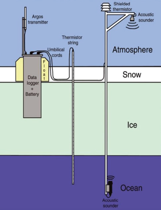
Schematic diagram of the instrumentation package of an International Arctic Buoy Programme (IABP) ice mass-balance buoy (IMB). Typically, IABP buoys record date, time, barometric pressure, surface temperature, air temperature, and water temperature and pressure at specific depths down to 60 meters below sea level. Diagram provided by C. Polashenski, Dartmouth College (from Polashenski and others, 2011, fig. 1); used with permission.
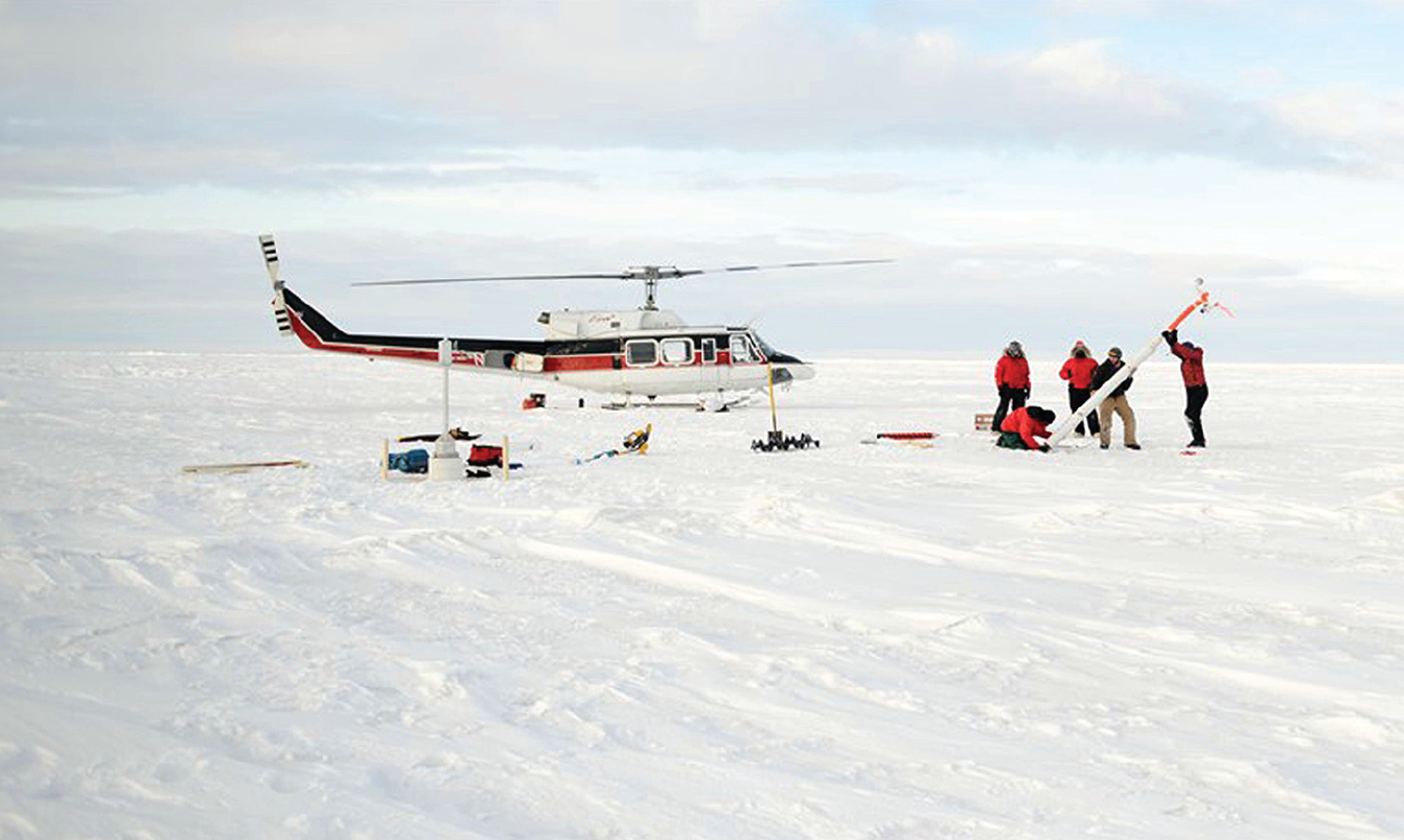
Photograph of an ice mass-balance buoy (IMB) used by the International Arctic Buoy Programme being prepared for deployment. Photograph provided by I. Rigor, University of Washington, used with permission.
Methods for Tracking Buoys
Until 2010, the Advanced Research and Global Observation Satellite (ARGOS) system was used to transmit data and buoy positions to the USGS. That year, the U.S. Army Cold Regions Research and Engineering Laboratory (CRREL), a U.S. logistics provider for the IABP, switched from ARGOS data transmission satellites to Iridium Communications transmission satellites. In 2011, GPS receivers and transmitters were added to the buoys equipped with Iridium Communications.
The IABP managers assisted the USGS by setting up a file transfer protocol (FTP) website that allowed the USGS to download buoy GPS data. With access to the buoy GPS data files, the USGS developed a methodology to convert the GPS data text files to a comma separated values (CSV) format and create an ArcGIS shapefile. The ArcGIS shapefile was then plotted within Esri’s ArcMap to plot out the latest buoy positions. By plotting the buoy track, USGS personnel saw how the wind and ocean currents affected buoy and associated ice floe movement. These plots aided in predicting where to task the next target location. Tasking is the formal process of determining and submitting the specific information necessary to correctly identify the location where a new image needs to be collected.
In the summer of 2008, the USGS successfully captured imagery of ice floes by using a target size of 4×4 nautical miles (nmi). This imagery demonstrated to the USGS, MEDEA, and the IABP that the USGS-developed methodology worked. In 2009, target sizes were modified to 10×10 nmi to maximize the amount of time the drifting buoy would be within the target area.
In 2009, the MEDEA Program asked the USGS to track the same ice floes over an entire season from April through September, over multiple sites (Wilson and others, 2012). In 2011, Python scripts were incorporated into the methodology to more quickly convert buoy GPS position text files to ArcGIS shapefiles. This development allowed the USGS to annually monitor and track more GPS buoys in support of the MEDEA Program.
The MEDEA Program scientists involved in cryosphere studies determined which areas of the Arctic needed to be studied. The IABP managers provided the locations of the GPS buoys. Together they determined which buoys in the IABP network the USGS would track and image. The IABP managers set up a website where selected Arctic buoy GPS data were updated hourly and stored. This was the primary source of information used by the USGS to track the buoys.
A buoy’s GPS text file contains the buoy’s ARGOS identification number, year, day, time, and latitude and longitude (fig. 12). This file information was updated hourly and was available on an FTP site for USGS collection managers to download and process into a geographic information system (GIS) format. These data were plotted to construct an ever-growing buoy track. The ArcGIS shapefile of the buoy track was used to estimate the displacement and direction of travel of the buoy.
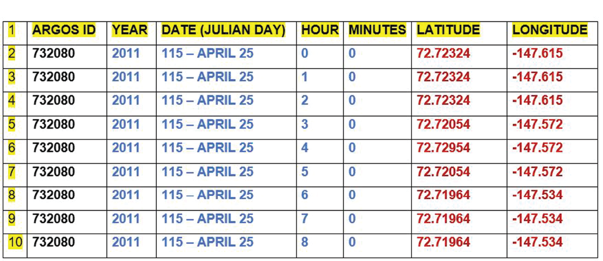
Example of a Global Positioning System (GPS) 8-hour text file from a buoy deployed by the International Arctic Buoy Programme (IABP). The buoy’s GPS text file contains the buoy’s Advanced Research and Global Observation Satellite system identification number (ARGOS ID), year, Julian day, time (hours [0-23] and minutes [0-59]), latitude, and longitude. These data were received hourly and downloaded from an IABP website for U.S. Geological Survey researchers to use.
The GPS buoy track of hourly records was plotted daily and was color coded by day (fig. 13). For example, all Monday positions were the same color, whereas the Tuesday positions were a different color, and so on.
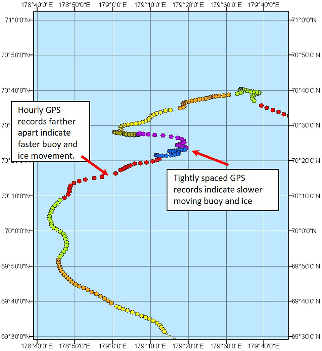
Example of a track map showing a plot of the Global Positioning System (GPS) locations of a buoy as it was tracked across the Arctic Ocean for 11 days. The plot is from an ArcGIS shapefile. Shapefiles of GPS position data were plotted in ArcMap so that U.S. Geological Survey (USGS) researchers could track buoys deployed by the International Arctic Buoy Programme. On track maps such as this one, circles representing hourly records were color coded for each day of the week; for example, Monday, red; Tuesday, blue; Wednesday, purple; Thursday, olive; Friday, yellow; Saturday, orange; Sunday, light green. Widely spaced circles indicate faster buoy movement than closely spaced circles. The map was produced by the USGS National Civil Applications Center in 2015.
The buoy movement was caused by prevailing winds and ocean currents pushing against the ice pack and ice floes. Because of this driving mechanism, the ice movement could be erratic. Alternatively, the buoy could travel for days in a straight line. To account for these variables, USGS collection managers plotted the buoy track daily.
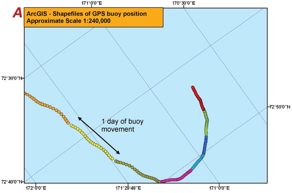
Next, the USGS used the buoy track plot to estimate a position for a target area. The challenging part was to position this target so that the buoy and therefore the surrounding sea ice would remain inside the target area for the next 2–3 days (fig. 14A, B). Estimates of the target position depended on the displacement rate and the direction in which the buoy and ice were moving. Sometimes, Arctic storms caused a buoy to move very quickly out of the target zone. The time of year also greatly affected buoy movements. For instance, in the spring when the sea ice was basically a large continuous sheet of pack ice, buoy and ice floe movements tended to be slower. As the year progressed, melt ponds and leads formed, and the ice began to melt and break apart. In late summer and early fall when sea ice extent was close to its minimum, there was more open water between ice floes. Buoys were pushed much greater distances, often at higher velocities. Plotting the GPS buoy track led to determining the displacement rate of the buoy, as the tighter the GPS spacing was between the hourly records (dots on a map), the slower the buoy was moving. Conversely, the farther apart the hourly GPS records, the faster the buoy and ice were moving.
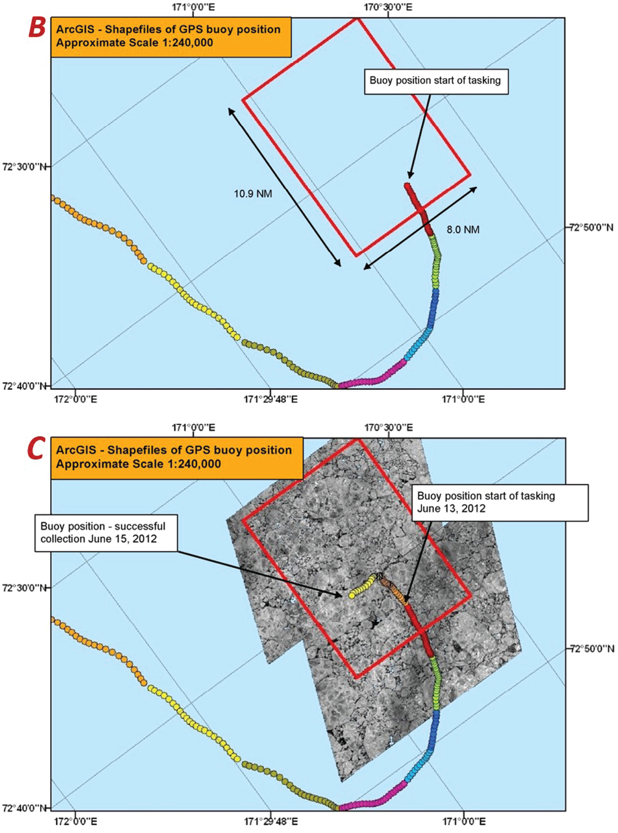
Maps showing the track of Advanced Research and Global Observation Satellite (ARGOS) system Buoy 82400 in the East Siberian Sea and imagery collected of part of the area traversed. A, Map showing hourly positions of ARGOS Buoy 82400 during a 8-day period in June 2012 (June 6–13). Global Positioning System (GPS) position data were plotted in ArcMap to represent the track, which was used to estimate the speed and direction of buoy and ice floe travel. B, Map showing the location of the tasking box (red rectangle) that was requested on the basis of the June 13, 2012, position of ARGOS Buoy 82400. The tasking box is the map area designated for collecting a satellite image of the buoy and surrounding ice. C, Map overlain by the images collected on June 15, 2012, in response to the tasking box shown in part B. The images are literal imagery-derived products (LIDPs) derived from U.S. National Imagery Systems electro-optical satellite images. The position of Buoy 82400 on that day was within the imaged area. On track maps such as these, circles representing hourly records of buoy positions were color coded for each day of the week. NM, nautical mile. The maps were produced by the U.S. Geological Survey National Civil Applications Center in 2015.
Figure 14C demonstrates the successful collection of an actual image captured 2 days after tasking. Receiving a cloud-free image of ice inside the projected target area constituted a successful collection. One reason that the USGS plotted the buoy track on an hourly and daily basis was to make sure that the buoy was still well inside the targeted area. If the buoy moved outside of the target zone, or even close to the edge of the target area, a new target position was calculated, plotted, and submitted for collection of future images. If a collected image had more clouds than was acceptable, the buoy track was checked against the target position, recalculated if necessary, and resubmitted for collection.
Occasionally, a GPS buoy stopped transmitting. This situation was caused by several different issues. The most likely cause was that the battery powering the GPS unit had run out of electrical power. In this case, the USGS contacted the IABP and MEDEA to identify an alternative buoy to target. Sometimes a buoy got caught up on an ice ridge, which caused the GPS transmission antenna to be tilted at an angle, resulting in the satellite relay not receiving the GPS signal. Sometimes the signal was blocked. In that situation, the USGS monitored the GPS website to see if the buoy resumed transmitting GPS data. If it did not transmit within a week, the USGS consulted with the IABP and MEDEA to switch collection to a new buoy. After the USGS downloaded an image, quality-assurance and quality-control steps were performed to confirm that the same ice floes were visible for each buoy being tracked.
For example, an image of the ice containing Buoy 132070 was taken on June 21, 2012 (fig. 15A), and compared to an image taken 32 days later on July 23, 2012 (fig. 15B), to make sure that the large dark ice mass, an unnamed ice island, was imaged in both scenes. It was. An oblique aerial photograph of the unnamed ice island had been taken more than a year earlier, on April 15, 2011. It is shown on figure 15C. The foreknowledge of the presence of the ice island was a factor in deciding the site of buoy placement.
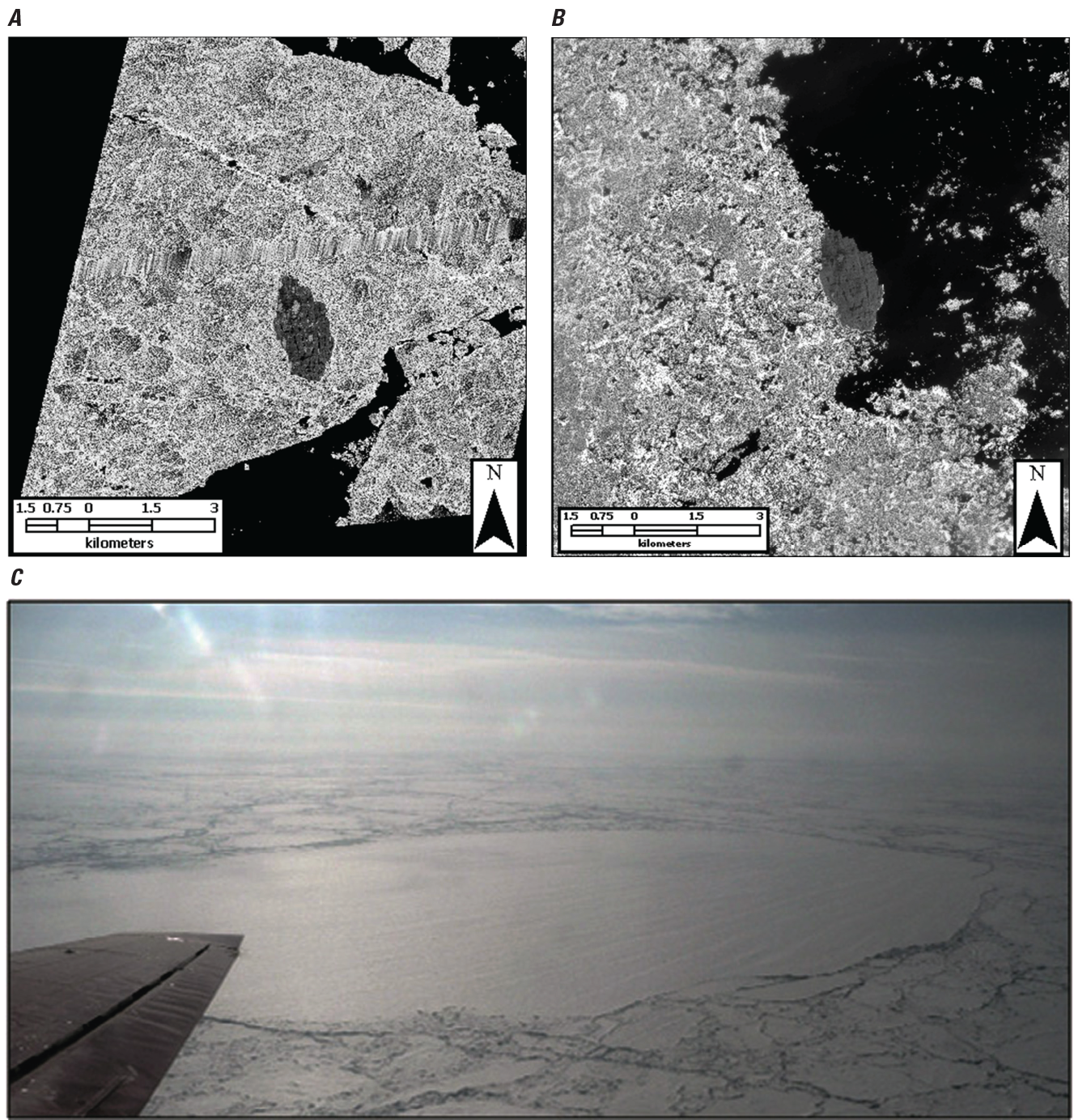
Two satellite images and an oblique aerial photograph of an unnamed Arctic Ocean ice island. A, A literal imagery-derived product (LIDP) derived from a U.S. National Imagery Systems electro-optical satellite image collected June 21, 2012, depicting an Arctic Ocean ice island and the adjacent sea ice. Advanced Research and Global Observation Satellite (ARGOS) system Buoy 132070 was installed on this ice island in the spring of 2012. The buoy is too small to be visible on the image. In parts A and B, the island appears dark gray, the surrounding sea ice is a mottled gray-white, and open water is black. Immediately north of the island, a band of distorted data extends across the entire image and represents an area about 0.25 kilometer (km) wide. The image area is about 10×10 km, while the ice island is about 2.7×1.3 km. B, An LIDP made from a satellite image collected 32 days later on July 23, 2012, of the same unnamed ice island and its surrounding sea ice shown in part A. Note the loss of sea ice in the upper right (northeast) quadrant of the image. C, Oblique aerial photograph taken April 15, 2011, of the ice island shown in parts A and B. The surface of the ice island is smooth, flat, and striated, while the adjacent sea ice appears hummocky and fractured. A detailed image time series showing changes in this ice island and its associated sea ice is shown in figure 18.
Usually, ice islands are not composed of sea ice. They are tabular icebergs of glacier origin, found in the Arctic Ocean, and they usually form by breaking off from an ice shelf. Ice islands typically are 30–50 m thick and occupy areas ranging from a few thousand square meters to 500 km2 (NSIDC, 2022b). Glacier ice and sea ice have different chemical and physical properties, including salinity, color, and surface texture.
Arctic ice islands typically calve from Canadian High Arctic ice shelves, primarily located along the north coast of Ellesmere Island. These Canadian High Arctic ice shelves are the only ice shelves in North America, and they are the most extensive ice shelves in the northern polar region. Ellesmere Island ice shelves originate from both glacier ice and sea ice (Jeffries, 1992).
Imagery Products From Sea Ice Buoys
Between 2009 and 2014, the USGS successfully tracked 38 different sea ice buoys and collected satellite images of the changes in the adjacent sea ice. The LIDPs of many of the resulting imagery products are available on the USGS GFLDAP website for free download and for unrestricted use. Table 2 summarizes the annual number of observed buoys and images collected.
Table 2.
Number of images collected from 38 buoys drifting in the Arctic Ocean between 2009 and 2014 and released to the Global Fiducials Library.[Data from the U.S. Geological Survey’s Global Fiducials Library Data Access Portal (https://www.usgs.gov/global-fiducials-library-data-access-portal),May 15, 2022]
The tracks of 38 buoys monitored between 2009 and 2014 are shown on figure 16. This figure depicts the general location, the path, and the complexity of the route that each individual buoy traveled during its period of observation. The USGS successfully imaged ice movement across hundreds or, in some cases, thousands of kilometers of the Arctic Ocean for periods from less than 2 months to, in one instance (IAPB Buoy 125530), more than 17 months. A description of some uses of drift buoy observations was presented in Kwok and Untersteiner (2011).
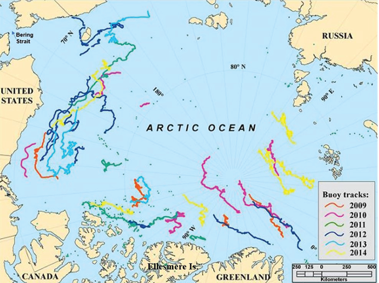
Map showing the tracks of the 38 drift buoys tracked by the U.S. Geological Survey (USGS) during the first 6 years (2009–2014) of the Global Fiducials Program’s Arctic Drift Buoy Sea Ice Study. Terms: E, East; N, North; and W, west. The map was produced by the USGS National Civil Applications Center in 2015.
Typically, imagery was analyzed by the USGS scientists, cooperators, and MEDEA scientists to determine ice fracture patterns, sea ice ridge heights, ice cover percentages, seasonal development and coverage of melt ponds, evolution of ice concentrations, floe size distribution, lateral melting, and other variables that are used to monitor sea ice extent and behavior and to refine and develop climate models. Resulting ice floe imagery has been added to the GFL for 38 buoys tracked from 2009 through 2014.
Case studies depicting the imagery for two drift buoys are presented below. These images demonstrated the timing and extent of melt pond development and allowed scientists to conduct comparative analysis studies to better understand seasonal changes and physical ice changes and processes that affected the same ice floes during the period of observation.
Case Study 1—Advanced Research and Global Observation Satellite Buoy 132070
ARGOS Buoy 132070, located on an unnamed ice island shown in figure 15C, was monitored between June 20, 2012, and September 24, 2012, and imaged between June 21, 2012, and September 21, 2012. During that 97-day monitoring period, Buoy 132070 drifted 1,570 km. The USGS GFLDAP website page for this buoy contains 15 LIDP images derived from images collected through September 21, 2012. This Beaufort Sea ice island was about 2.7 km long by 1.3 km wide when first imaged. Figure 17 is a map showing the westerly track the ice island and buoy followed from north of the United States-Canada border to north of the Bering Strait.
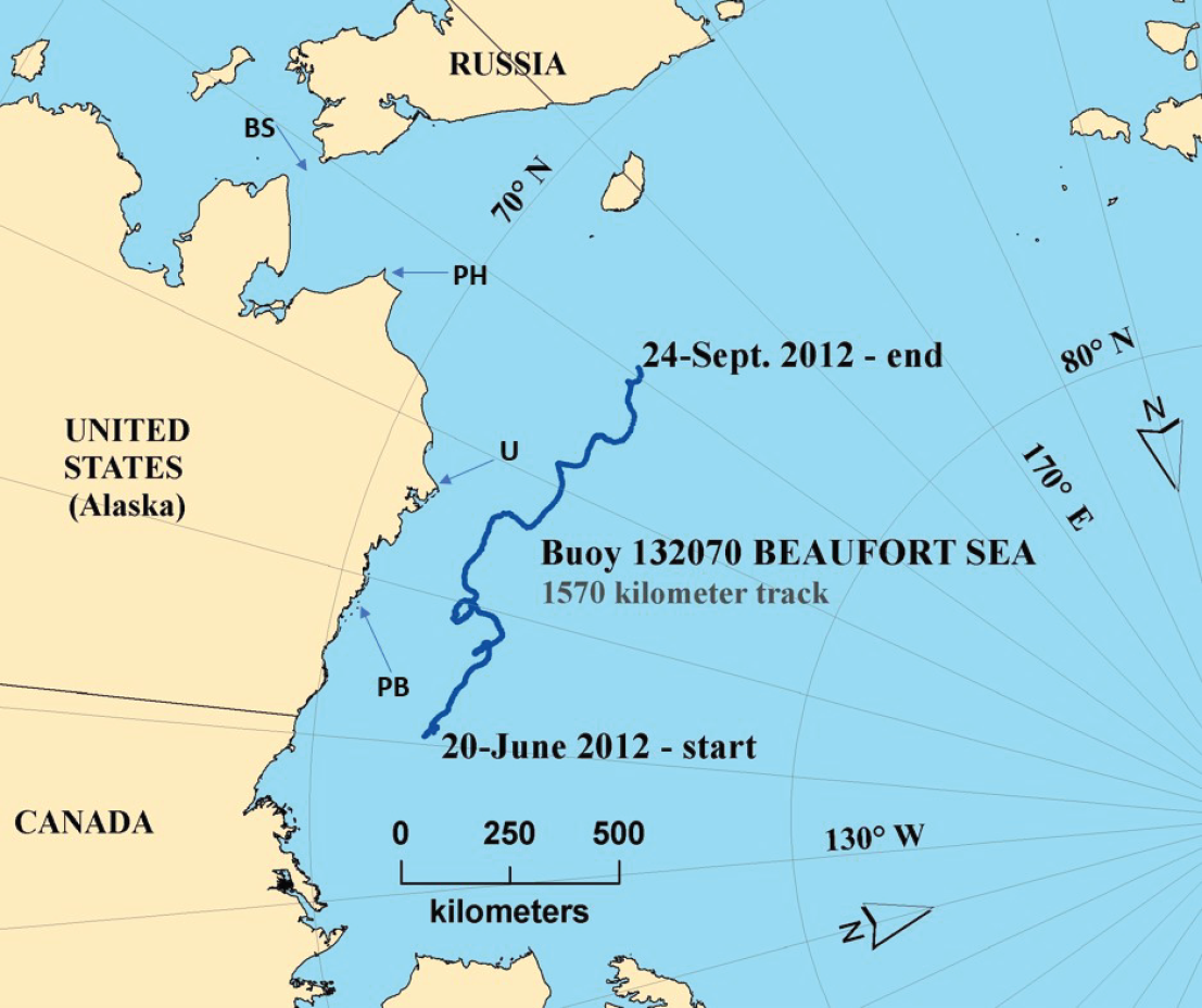
Map showing the westerly track of the unnamed ice island containing Advanced Research and Global Observation Satellite (ARGOS) system Buoy 132070 as it drifted from June 20, 2012, through September 24, 2012, in the Beaufort Sea from north of the United States-Canada border to north of the Bering Strait. Terms: BS, Bering Strait; E, East; N, North; PB, Prudhoe Bay; PH, Point Hope; U, Utqiagvik; and W, West. The map was produced by the U.S. Geological Survey National Civil Applications Center in 2015.
Figure 18 contains eight LIDP images derived from USNIS electro-optical images of the ice containing ARGOS Buoy 132070; the images were collected during the 48-day period between June 21 and August 7, 2012. All have been degraded for public release. Each image depicts an area that was 3.1 km from east to west by 3.6 km from north to south. The images show the changes that the unnamed ice island and adjacent sea ice experienced as they drifted to the west during the summer of 2012.
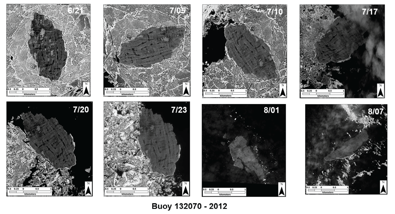
Eight annotated images of the ice island containing Advanced Research and Global Observation Satellite (ARGOS) system Buoy 132070 and its adjacent sea ice that were collected during the 48-day period between June 21 and August 7, 2012. These literal imagery-derived products (LIDPs) were derived from United States National Imagery Systems electro-optical satellite images. All have been degraded for public release. Each image depicts an area that was approximately 3.1 kilometers (km) from east to west by 3.6 km from north to south. The images show the changes that the unnamed ice island (dark gray) and adjacent sea ice (white) experienced as they drifted to the west in the Beaufort Sea during the summer of 2012. The LIDPs are from the Global Fiducials Library Data Access Portal (https://www.usgs.gov/global-fiducials-library-data-access-portal).
As shown in the image collected on June 21 (6/21 on fig. 18), the ice island, which had a dark-gray surface cut by subparallel fractures or crevasses, was oriented nearly north-south. The area surrounding it was composed of tightly packed angular ice floes with only four small areas of open water. Much of this area was snow covered with a mottled appearance, probably due to the presence of small melt ponds.
The image collected 15 days later, on July 5 (7/05 on fig. 18), showed that the ice island had rotated nearly 90° to the east. The former northern end was pointing to the northeast. The surrounding area was still composed of tightly packed angular ice floes. The southwestern corner of the area imaged had a large area of open water. Most of the snow was gone, and the number of small melt ponds had increased. A lead was beginning to form at what previously was the south end of the ice island.
The image collected 5 days later, on July 10 (7/10 on fig. 18), showed that the continued rotation of the ice island had resulted in the former northern end pointing to the southeast. Most of the surrounding area was still composed of tightly packed angular ice floes, but an area of open water measuring about 1.0×1.5 km had developed on the west side of the ice island. Most of the remaining snow was located between ice floes. The number of small melt ponds had continued to increase.
The image collected 7 days later, on July 17 (7/17 on fig. 18), showed that the former northern end was again pointing to the northeast. The direction of its rotation was unknown. Only the western part of the surrounding area was composed of tightly packed angular ice floes. The entire eastern area was open water. The size of the melt ponds had continued to increase.
The image collected 3 days later, on July 20 (7/20 on fig. 18), showed that the former northern end was pointing to the southeast, and the island’s area was decreasing due to calving and melting. Most of the western part of the surrounding area was composed of tightly packed angular ice floes with several large areas of open water. The entire eastern area was open water. The area of the melt ponds had continued to increase.
The image collected 3 days later, on July 23 (7/23 on fig. 18), showed that the former northern end was pointing to the south-southeast, yet the ice island had changed very little. Most of the western part of the surrounding area was composed of tightly packed angular ice floes with fewer areas of open water than on July 20. The entire eastern area was still open water. The area of the melt ponds had continued to increase.
The image collected 9 days later, on August 1 (8/01 on fig. 18), showed that more than half of the ice island present on July 23 had calved and melted away. Only a few small ice floes remained. The remaining area was open water.
The image collected 6 days later, on August 7 (8/07 on fig. 18), showed that the remaining piece of the ice island had continued to calve and melt. The remaining fragment, which was now about 0.7×1.9 km, had rotated nearly 90° to the west. Only a few small ice floes remained.
Although images used here extend through August 7, imaging continued through September 21, and position monitoring of the few remaining fragments of the ice island continued until September 24, 2012.
Case Study 2—World Meteorological Organization Buoy 47611
The World Meteorological Organization (WMO) Buoy 47611, located in the Beaufort Sea, was monitored from June 20, 2009, to September 24, 2009, and imaged from June 27, 2009, to September 14, 2009. During that 79-day imaging period, the buoy drifted nearly 800 km. The USGS GFLDAP website page for this buoy contains 49 unique LIDP images derived from images collected by the USNIS through September 14, 2009.
Figure 19 is a map showing the westerly track that WMO Buoy 47611 followed as it drifted from northeast of the United States-Canada border to north of Alaska.
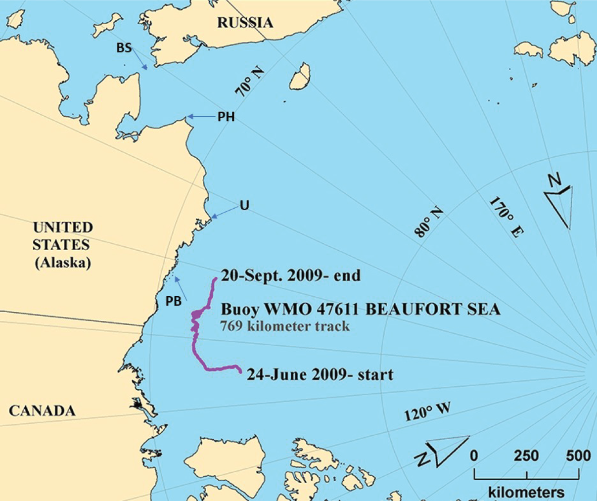
Map showing the westerly track of the sea ice containing World Meteorological Organization (WMO) Buoy 47611 as it drifted from June 24, 2009, through September 20, 2009, in the Beaufort Sea from northeast of the United States-Canada border to northeast of Utqiagvik (formerly Barrow), Alaska. Terms: BS, Bering Strait; E, East; N, North; PB, Prudhoe Bay; PH, Point Hope; U, Utqiagvik; and W, West. The map was produced by U.S. Geological Survey National Civil Applications Center in 2015.
Figure 20 contains 10 LIDP images derived from USNIS electro-optical satellite images of the ice containing WMO Buoy 47611 that were collected between June 27, 2009, and August 11, 2009. All have been degraded for public release. Each image depicts an area that was approximately 6.4 km from east to west by 6.8 km from north to south.
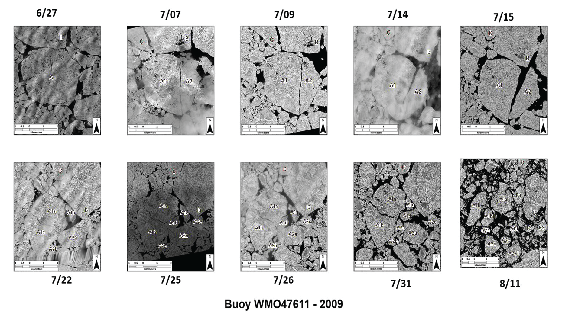
Ten images of the ice containing the World Meteorological Organization (WMO) Buoy 47611 that were collected between June 27, 2009, and August 11, 2009. These literal imagery-derived products (LIDPs) were derived from United States National Imagery Systems electro-optical satellite images. All have been degraded for public release. Each image depicts an area that was approximately 6.4 kilometers (km) from east to west by 6.8 km from north to south in the Beaufort Sea. The images show the changes that the monitored sea ice experienced as it drifted to the west during the 48-day period depicted in the figure. The LIDPs are from the Global Fiducials Library Data Access Portal (https://www.usgs.gov/global-fiducials-library-data-access-portal). Labels (A, B, C) identify the floes and their daughter products (smaller fragments), which have labels such as “A1b” and “B2.”
The images show the changes that the monitored sea ice experienced as it drifted to the west during the 48-day period depicted in the figure. On June 27, 2009 (6/27 on fig. 20), the monitored area contained more than a dozen large subrounded to angular composite ice floes. They ranged in maximum dimension from less than 0.25 km to more than 3.0 km. The two largest ice floes were labeled “A” and “B.” Only a part of floe B can be seen. Less than 15 percent of the area was open water. Some of the ice was snow covered with a mottled appearance, probably due to the presence of small melt ponds. Cloud shadows and small areas of sunshine provide a false hummocky texture to parts of the image.
The image collected 10 days later, on July 7, 2009 (7/07 on fig. 20), showed that most of the large composite ice floes described above changed minimally. A north-south fracture in composite ice floe A had resulted in the separation of its eastern third. To facilitate tracking, the two fragments were labeled “A1” and “A2.” Some of the smaller floes had fractured, producing many smaller fragments. Overall, the area of open water had increased slightly. The greatest change was northeast of floe A2. Cloud shadows and small areas of sunshine continued to provide a false hummocky texture to parts of the image. A large floe on the northwest corner of the image was labeled “C.”
The image collected 2 days later on July 9, 2009 (7/09 on fig. 20), showed an area that was cloud free. As in earlier images, most of the large composite ice floes showed minimal changes. Little change had occurred at the north-south fracture separating floes A1 and A2. Additional smaller floes had fractured, producing more fragments. The area of open water had continued to increase. The greatest change remained northeast of floe A2.
The image collected 5 days later on July 14, 2009 (7/14 on fig. 20), showed an area that was more than 90-percent cloud covered. However, the clouds were thin to the extent that they ranged between transparent and translucent. The most significant change that is visible from the previous image is at the north-south fracture separating floe fragments A1 and A2. Fragment A2 had begun to rotate toward the southeast, and as much as 0.2 km of separation had occurred at the north end of the fracture.
The image collected the next day, July 15, 2009 (7/15 on fig. 20), showed an area that was 100-percent cloud free. The most significant change was still the result of the continuing rotation of floe A2 along the north-south fracture separating floes A1 and A2. Maximum separation was about 0.6 km. Fragment A2 had drifted northward as it rotated toward the southeast. Melt ponds were the most significant surface feature on the ice floes.
The image collected on July 22, 2009 (7/22 on fig. 20), showed significant cloud cover and a band of lost data. In the 7 days between images, ice floes A1 and A2 each had broken into multiple fragments, although the fragments remained in close proximity to each other. The entire ice mass had rotated clockwise about 15°.
The image collected 3 days later, on July 25, 2009 (7/25 on fig. 20), showed an area that was cloud free. There was very little difference between ice floes A1 and A2 and their daughter products shown in this image compared with the previous image. Similarly, floes B and C showed minimal change since they were first described.
The image collected 1 day later, on July 26, 2009 (7/26 on fig. 20), had a band of cloud cover in mid-image. Compared to the previous image, this image shows very little difference between ice floes A1 and A2 and their daughter products. Similarly, floes B and C showed very little change.
The image collected 5 days later, on July 31, 2009 (7/31 on fig. 20), is cloud free. Surface snow cover and melt pond area were significantly less than previously shown. Since July 26, 2009, the amount of open water had increased by about 15 percent. Only small changes had occurred to ice floes A1 and A2 and their daughter products. While ice floe B continued to show very little change, the southwest side of ice floe C had fractured.
The final image in this sequence, collected 11 days later on August 11, 2009 (8/11 on fig. 20), is also cloud free. Open water covered about 40 percent of the area shown. Since July 31, all of the labeled ice floes except C had developed many fractures. The length of the largest fragment of floe B exceeded 3.0 km. Subsequent imagery showed the continued decrease in size of all ice floes. The final image, not shown here, was collected 34 days later, on September 14, 2009.
Imagery From Seasonal Ice Zone Sites
The Seasonal Ice Zone (SIZ) is the region between maximum winter sea ice extent and minimum summer sea ice extent. As such, it contains the full range of positions of the Marginal Ice Zone (MIZ), where sea ice interacts with open water. The long-term goal of the Seasonal Ice Zone Reconnaissance Surveys (SIZRS) Program is to track and understand the interplay among the ice, atmosphere, and ocean contributing to the rapid decline in summer ice extent that has occurred in recent years.
The overarching objectives for SIZRS are listed below as they were described by Morrison (2017, p. 1):
-
• Determine seasonal variations in air-ice-ocean characteristics across the SIZ extending over several years and for a variety of SIZ conditions;
-
• Investigate and test hypotheses about the physical processes that occur within the SIZ that require data from all components of SIZRS; and
-
• Improve predictive models of the SIZ through model validation and through the determination of observing system requirements.
The GFP has released more than 300 sea ice LIDP images derived from images collected by the USNIS in 2013 and 2014 in support of the SIZRS Program. The program is managed by the University of Washington’s Polar Science Center and is described on the center’s website as “a coordinated program of repeated ocean, ice, and atmospheric measurements across the Beaufort-Chukchi Sea seasonal sea ice zone (SIZ)” (University of Washington, Polar Science Center, 2022c). Through 2014, the last year for which GFP imagery is available, sites were imaged at every degree of latitude between 70° and 80° N. along a north-south transect.
Summary
Since 1997, the Global Fiducials Program (GFP) has collected remotely sensed high-resolution United States National Imagery Systems (USNIS) imagery to monitor Arctic sea ice behavior. Initial imagery collection efforts documented the Surface Heat Budget of the Arctic Ocean (SHEBA) Project, in which the Canadian icebreaker, Des Groseilliers was purposely frozen into sea ice of the Beaufort Sea. This Arctic sea ice project spanned 404 days, from August 25, 1997, to October 3, 1998, with the icebreaker serving as a platform for experiments and a base for scientific research. More than 100 USNIS images were acquired of the ship and the ice adjacent to it as the ship drifted across the Beaufort Sea.
Fifty-seven (57) of the images were publicly released as literal imagery-derived products (LIDPs) having a resolution of 1.3 meters. An LIDP is an image-like product that is not a direct copy of the original image. LIDPs have had their pixels digitally manipulated so that the pixels’ original characteristics are irreversibly changed while the appearance of the image remains unchanged. This manipulation is done to prevent adversaries from determining the capabilities of the sensors that collected the original image.
Beginning in 1999, six static sea ice sites in the Arctic Ocean were imaged for periods as long as 15 years in order to better understand sea ice dynamics, distribution, age, melt history, and annual variability. The sites were located (1) in the Chukchi Sea; (2) offshore of Barrow (now Utqiagvik), Alaska; (3) in the Beaufort Sea; (4) in the Canada Basin; (5) in the Fram Strait; and (6) in the East Siberian Sea. Between 1999 and 2014, the number of static site images approved for public release was 884.
In 2009, the U.S. Geological Survey (USGS) began to track and repeatedly capture imagery of the same ice over time as it drifted across the Arctic Ocean. The study method was to track telemetering buoys at various locations across the Arctic. Between 2009 and 2014, 38 buoys were monitored for periods ranging from less than 2 months to more than 17 months. The buoys and associated sea ice drifted across hundreds or, in some cases, thousands of kilometers of the Arctic Ocean during the periods of collection. A total of 1,734 LIDP images derived from USNIS images collected from tracking 38 unique buoys have been approved for public release.
In 2013 and 2014, in support of the Seasonal Ice Zone Reconnaissance Surveys (SIZRS) Program, the USGS imaged sites in the Beaufort and Chukchi Seas located at every degree of latitude between 70° and 80° N. along a north-south transect. This was done to track and understand the interplay among the ice, atmosphere, and ocean contributing to the rapid decline in summer ice extent that has occurred in recent years. In support of this goal, more than 300 sea ice LIDP images have been approved for public release.
For each of these efforts, resulting sea ice imagery products approved for public release are posted on two websites hosted by the USGS for the Global Fiducials Program:
-
• Global Fiducials Library (GFL) website, which has an image gallery at https://gfl.usgs.gov/imagegallery/?PTAGNAME=ArcticBuoys&img:2573:208, and
-
• Global Fiducials Library Data Access Portal website at https://www.usgs.gov/global-fiducials-library-data-access-portal.
References Cited
Baker, D.J., and Zall, L., 2020, The MEDEA Program—Opening a window into new Earth science data: Oceanography, v. 33, no. 1, p. 20–31, accessed May 15, 2022, at https://doi.org/10.5670/oceanog.2020.104.
Comiso, J.C., Parkinson, C.L., Markus, T., Cavalieri, D.J., and Gersten, R., 2022, Current state of sea ice cover: National Aeronautics and Space Administration, Goddard Earth Sciences Division Projects website, accessed October 25, 2022, at https://earth.gsfc.nasa.gov/cryo/data/current-state-sea-ice-cover.
Dozier, J., 1997, Environmental study and monitoring with classified satellite data [abs.]: Goddard Space Flight Center Engineering Colloquium, September 15, 1997, lecture abstract, accessed May 15, 2022, at https://ecolloq.gsfc.nasa.gov/archive/1997-Fall/announce.dozier.html.
Fetterer, F., and Untersteiner, N., 1998, Observations of melt ponds on Arctic sea ice: Journal of Geophysical Research, v. 103, no. C11, p. 24821–24835, accessed May 15, 2022, at https://agupubs.onlinelibrary.wiley.com/doi/abs/10.1029/98JC02034.
Fetterer, F., and Untersteiner, N., 2000, SHEBA reconnaissance imagery, version 1—Data set G02180: National Snow and Ice Data Center website, accessed May 15, 2022, at https://nsidc.org/data/G02180/versions/1.
Fetterer, F., Wilds, S., and Sloan, J., 2008, Arctic sea ice melt pond statistics and maps, 1999–2001, version 1—Data set G02159: National Snow and Ice Data Center website, accessed May 15, 2022, at https://nsidc.org/data/g02159.
Jeffries, M.O., 1992, Arctic ice shelves and ice islands—Origin, growth and disintegration, physical characteristics, structural-stratigraphic variability, and dynamics: Reviews of Geophysics, v. 30, no. 3, p. 245–267, accessed May 15, 2022, at https://agupubs.onlinelibrary.wiley.com/doi/10.1029/92RG00956.
Kwok, R., and Untersteiner, N., 2011, New high-resolution images of summer Arctic sea ice: Eos, Transactions, American Geophysical Union, v. 92, no. 7, p. 53–54, accessed May 15, 2022, at https://doi.org/10.1029/2011EO070002.
Meier, W.N., Fetterer, F., Savoie, M., Mallory, S., Duerr, R., and Stroeve, J., 2017, NOAA/NSIDC climate data record of passive microwave sea ice concentration, version 3—Data set G02202: National Snow and Ice Data Center website, accessed May 15, 2022, at https://nsidc.org/data/G02202/versions/3.
Molnia, B.F., Angeli, K.M., and Dilles, S.J., 2018, Using Global Fiducial Program imagery to better understand and manage the geology and hydrology of public lands [abs.], in Geological Society of America Annual Meeting, November 4–7, 2018, Indianapolis, Indiana: Geological Society of America Abstracts with Programs, v. 50, no. 6, accessed May 15, 2022, at https://doi.org/10.1130/abs/2018AM-320083.
Molnia, B.F., Price, S.D., and, King, S.E., 2012, Global Fiducials Program imagery—New opportunities for geospatial research, outreach, and education [abs.]: American Geophysical Union, Fall Meeting 2012, abstract id. ED34A-01, accessed May 15, 2022, at https://ui.adsabs.harvard.edu/abs/2012AGUFMED34A..01P/abstract.
Morrison, J., 2017, Ocean profile measurements during the Seasonal Ice Zone Reconnaissance Surveys Ocean Profiles: Final Technical Report, prepared for the Office of Naval Research for grant N00014–12–1–0236, 8 p., accessed May 15, 2022, at https://apps.dtic.mil/sti/pdfs/AD1026542.pdf.
Nansen, F., 1897, Farthest north—Being the record of a voyage of exploration of the ship “Fram” 1893–96 and of a fifteen months’ sleigh journey by Dr. Nansen and Lieut. Johansen: New York, Harper & Brothers Publishers, v. I, 120 p., accessed May 15, 2022, at https://archive.org/details/farthestnorthbe06svergoog/page/n10/mode/2up.
National Center for Atmospheric Research, [undated], SHEBA—Surface Heat Budget of the Arctic Ocean: National Center for Atmospheric Research, Earth Observing Laboratory website, accessed May 15, 2022, at https://www.eol.ucar.edu/field_projects/sheba.
National Centers for Environmental Information [NCEI], 2021, NOAA delivers new U.S. climate normals: National Oceanic and Atmospheric Administration news release published May 4, 2021, and updated May 5, 2021, accessed January 28, 2023, at https://www.ncei.noaa.gov/news/noaa-delivers-new-us-climate-normals.
National Science Foundation, 1998, SHEBA breaks free of Arctic’s icy embrace: National Science Foundation news release 98–068, accessed December 19, 2022, at https://www.nsf.gov/news/news_summ.jsp?cntn_id=102932.
National Science Foundation, 2000, SHEBA Program—Nifty 50, article 42 of Nifty 50 [articles published for the NSF’s 50th anniversary celebration]: National Science Foundation website, accessed May 15, 2022, at https://www.nsf.gov/about/history/nifty50/sheba.jsp.
National Snow and Ice Data Center [NSIDC], 2012, Arctic sea ice extent settles at record seasonal minimum: National Snow and Ice Data Center, Arctic Sea Ice News and Analysis web page, accessed May 15, 2022, at https://nsidc.org/arcticseaicenews/2012/09/arctic-sea-ice-extent-settles-at-record-seasonal-minimum/.
National Snow and Ice Data Center [NSIDC], 2022a, Charctic interactive sea ice graph—Arctic sea ice extent: National Snow and Ice Data Center, Arctic Sea Ice News and Analysis website, accessed September 8, 2022, at https://nsidc.org/arcticseaicenews/charctic-interactive-sea-ice-graph/.
National Snow and Ice Data Center [NSIDC], 2022b, Cryosphere glossary: National Snow and Ice Data Center website, accessed May 15, 2022, at https://nsidc.org/cryosphere/glossary/.
National Snow and Ice Data Center [NSIDC], 2022c, The Arctic Ice Dynamics Joint Experiment (AIDJEX): National Snow and Ice Data Center web page, accessed May 15, 2022, at https://nsidc.org/noaa/aidjex.
National Snow and Ice Data Center [NSIDC], 2023, Cryosphere glossary: National Snow and Ice Data Center website, accessed January 28, 2023, at https://nsidc.org/learn/cryosphere-glossary/ice-extent.
Opstal, D.W., and Rogers, R.T., 2022, Civil Applications Committee (ver. 1.1, February 2022): U.S. Geological Survey Fact Sheet 2022–3002, 2 p., accessed May 15, 2022, at https://pubs.usgs.gov/fs/2022/3002/fs20223002.pdf.
Peng, G., Meier, W.N., Scott, D.J., and Savoie, M.H., 2013, A long-term and reproducible passive microwave sea ice concentration data record for climate studies and monitoring: Earth System Science Data, v. 5, no. 2, p. 311–318, accessed May 15, 2022, at https://doi.org/10.5194/essd-5-311-2013.
Planck, C.J., Whitlock, J., Polashenski, C., and Perovich, D., 2019, The evolution of the seasonal ice mass balance buoy: Cold Regions Science and Technology, v. 165, article 102792, 8 p., accessed November 15, 2022, at https://doi.org/10.1016/j.coldregions.2019.102792.
Polashenski, C., Perovich, D., Richter-Menge, J., and Elder, B., 2011, Seasonal ice mass-balance buoys—Adapting tools to the changing Arctic: Annals of Glaciology, v. 52, no. 57, p. 18–26, accessed November 18, 2022, at https://doi.org/10.3189/172756411795931516.
Richter-Menge, J.A., Perovich, D.K., Elder, B.C., Claffey, K., Rigor, I., and Ortmeyer, M., 2006, Ice mass-balance buoys—A tool for measuring and attributing changes in the thickness of the Arctic sea-ice cover: Annals of Glaciology, v. 44, p. 205–210, accessed November 18, 2022, at https://doi.org/10.3189/172756406781811727.
University of Washington, Polar Science Center, [2022a], International Arctic Buoy Programme—About the maps: University of Washington, Polar Science Center website, accessed November 15, 2022, at https://iabp.apl.uw.edu/maps.html.
University of Washington, Polar Science Center, [2022b], International Arctic Buoy Programme—Overview: University of Washington, Polar Science Center website, accessed May 15, 2022, at https://iabp.apl.uw.edu.
University of Washington, Polar Science Center, [2022c], Seasonal Ice Zone Reconnaissance Surveys (SIZRS): University of Washington, Polar Science Center website, accessed May 15, 2022, at http://psc.apl.uw.edu/research/projects/sizrs/.
University of Washington, Polar Science Center, [2022d], UpTempO—Measuring the Upper layer Temperature of the Polar Oceans: University of Washington, Polar Science Center website, accessed November 15, 2022, at psc.apl.washington.edu/UpTempO/.
U.S. Geological Survey, 2022, Global Fiducials Library Data Access Portal: U.S. Geological Survey website, accessed May 15, 2022, at https://www.usgs.gov/global-fiducials-library-data-access-portal.
U.S. Joint Chiefs of Staff, 2017, Geospatial intelligence in joint operations: Joint Chiefs of Staff, Joint Publication 2–03 (July 5, 2017), variously paged [102 p.], accessed May 15, 2022, at https://www.jcs.mil/Portals/36/Documents/Doctrine/pubs/jp2_03_20170507.pdf. [Supersedes Joint Publication 2–03, “Geospatial Intelligence Support to Joint Operations,” version of October 31, 2012.]
Uttal, T., Curry, J.A, McPhee, M.G., Perovich, D.K., Moritz, R.E., Maslanik, J.A., Guest, P.S., Stern, H.L., Moore, J.A., Turenne, R., Heiberg, A., Serreze, M.C., Wylie, D.P., Persson, O.G., Paulson, C.A, Halle, C., Morison, J.H., Wheeler, P.A., Makshtas, A., Welch, H., Shupe, M.D., Intrieri, J.M., Stamness, K., Lindsey, R.W., Pinkel, R., Pegau, W.S., Stanton, T.P., and Grenfeld, T.C., 2002, Surface Heat Budget of the Arctic Ocean: Bulletin of the American Meteorological Society, v. 83, no. 2, p. 255–276, accessed May 15, 2022, at https://doi.org/10.1175/1520-0477(2002)083<0255:SHBOTA>2.3.CO;2.
Wilson, E.M., Wilds, S.R., Friesen, B.A., and Sloan, J.L., 2012, Global Fiducials Program—Arctic buoy sea ice studies [abs.]: American Geophysical Union, Fall Meeting 2012, abstract id. ED34A-03, accessed May 15, 2022, at https://ui.adsabs.harvard.edu/abs/2012AGUFMED34A..03W/abstract.
Woods Hole Oceanographic Institution, 2022, Ice tethered profilers: Woods Hole Oceanographic Institution website, accessed November 15, 2022, at https://www2.whoi.edu/site/itp/.
Abbreviations
AIDJEX
Arctic Ice Dynamics Joint Experiment
ARGOS
Advanced Research and Global Observation Satellite
CAC
Civil Applications Committee
CIA
Central Intelligence Agency
CRREL
U.S. Army Cold Regions Research and Engineering Laboratory
CSV
comma separated values
DMSP
U.S. Defense Meteorological Satellite Program
FTP
file transfer protocol
GFL
Global Fiducials Library
GFLDAP
Global Fiducials Library Data Access Portal
GFP
Global Fiducials Program
GFWG
Global Fiducials Working Group
GIS
geographic information system
GPS
Global Positioning System
IABP
International Arctic Buoy Programme
IDP
imagery-derived product
IMB
ice mass-balance
ITP
ice tethered profiler
km
kilometer
km2
square kilometer
LIDP
literal imagery-derived product
m
meter
MIZ
Marginal Ice Zone
NASA
National Aeronautics and Space Administration
NIC
U.S. National Ice Center
NM
nautical mile
nmi
nautical mile
NSF
National Science Foundation
NSIDC
National Snow and Ice Data Center
ONR
U.S. Office of Naval Research
SHEBA
Surface Heat Budget of the Arctic Ocean
SIZ
Seasonal Ice Zone
SIZRS
Seasonal Ice Zone Reconnaissance Surveys
SMMR
Scanning Multichannel Microwave Radiometer
UpTempO
Upper layer Temperature of the Polar Oceans
USGS
U.S. Geological Survey
USNIS
United States National Imagery Systems
WCRP
World Climate Research Programme
WMO
World Meteorological Organization
WWW
World Weather Watch Programme
Disclaimers
Any use of trade, firm, or product names is for descriptive purposes only and does not imply endorsement by the U.S. Government.
Although this information product, for the most part, is in the public domain, it also may contain copyrighted materials as noted in the text. Permission to reproduce copyrighted items must be secured from the copyright owner.
Suggested Citation
Molnia, B.F., and Wilson, E.M., 2023, Documenting Arctic sea ice dynamics with Global Fiducials Program imagery: U.S. Geological Survey Open-File Report 2023–1008, 32 p., https://doi.org/10.3133/ofr20231008.
ISSN: 2331-1258 (online)
| Publication type | Report |
|---|---|
| Publication Subtype | USGS Numbered Series |
| Title | Documenting Arctic sea ice dynamics with Global Fiducials Program imagery |
| Series title | Open-File Report |
| Series number | 2023-1008 |
| DOI | 10.3133/ofr20231008 |
| Publication Date | March 10, 2023 |
| Year Published | 2023 |
| Language | English |
| Publisher | U.S. Geological Survey |
| Publisher location | Reston, VA |
| Contributing office(s) | National Civil Applications Center |
| Description | viii, 32 p. |
| Online Only (Y/N) | Y |
| Additional Online Files (Y/N) | N |