

Calibration of the Trinity River Stream Salmonid Simulator (S3) with Extension to the Klamath River, California, 2006–17
Links
- Document: Report (7.7 MB pdf) , HTML , XML
- Download citation as: RIS | Dublin Core
Abstract
The Trinity River is managed in two sections: (1) the upper 64-kilometer (km) “restoration reach” downstream from Lewiston Dam and (2) the 120-km lower Trinity River downstream from the restoration reach. The Stream Salmonid Simulator (S3) has been previously constructed and calibrated for the restoration reach. In this report, we extended and parameterized S3 for the 120-km section of the lower Trinity River to the confluence with the Klamath River and then to the Pacific Ocean in northern California.
S3 is a deterministic life-stage structured-population model that tracks daily growth, movement, and survival of juvenile salmon. A key theme of the model is that river discharge affects habitat availability and capacity, which in turn drives density-dependent population dynamics. To explicitly link population dynamics to habitat quality and quantity, the river environment is constructed as a one-dimensional series of linked habitat units, each of which has an associated daily timeseries of discharge, water temperature, and useable habitat area or carrying capacity. In turn, the physical characteristics of each habitat unit and the number of fish occupying each unit drive (1) survival and growth within each habitat unit and (2) movement of fish among habitat units.
The physical template of the Trinity River was formed by classifying the river into 910 meso-habitat units that were designated into runs, riffles, or pools. For each habitat unit, we developed a timeseries of daily discharge, water temperature, amount of available spawning habitat, and fry and parr carrying capacity. Capacity timeseries were constructed using state-of-the-art models of spatially explicit hydrodynamics and quantitative fish habitat relationships developed for the Trinity River. These variables were then used to drive population dynamics such as egg maturation and survival, and in turn, juvenile movement, growth, and survival.
We estimated key movement and survival parameters by calibrating the model to 12 years (2007–18) of weekly juvenile abundance estimates from two rotary screw traps: (1) the Pear Tree trap near the downstream end of the restoration reach and (2) the Willow Creek trap site is about 40.2 km upriver from the Trinity River’s confluence with the Klamath River. The calibration consisted of replicating historical conditions as closely as possible (for example: flow, temperature, spawner abundance, spawning location and timing, and hatchery releases), and then running the model to predict weekly abundance passing the trap location. We also evaluated four alternative model structures that included either no density-dependence, density-independent movement and survival, density-dependent survival, or density-dependent movement. Akaike information criterion model selection was used to evaluate the strength of evidence for alternative model structures to simulate the observed abundance estimates.
Model selection supported the conclusion that the fully density-dependent model and density-dependent survival model was better supported by the data than the no density-dependence or density-dependent movement model. Because density-dependent movement was favored in past evaluations, we focus on the results from the fully density-dependent model. Parameter estimates from this model indicated that fry were less likely than parr to move downstream and that fry moved slower. Fry had a lower daily survival probability than parr. In contrast, hatchery fish had the highest probability of movement and the lowest daily survival probability.
Fitting the model to both traps individually enabled us to independently compare the fit and performance of S3 at simulating fish abundance, timing, and growth of juvenile salmon in the upper restoration reach and lower Trinity River. We obtained a better fit to the data at the Willow Creek trap site than we obtained at the Pear Tree trap site, regardless of whether we fit the model to the abundances at the Pear Tree trap or Willow Creek trap. This better fit was surprising given that the S3 input data for the upper restoration reach required fewer assumptions than fitting to the Willow Creek trap site that is farther down river. Fitting S3 to weekly abundances at the Willow Creek trap site required making assumptions about (1) extrapolating capacity-flow relationships to unmeasured habitat units; (2) spatially allocating spawners within the lower Trinity River; and (3) approximating the abundance, timing, and size of juveniles entering from tributaries. The model provided better fit to the data at the Willow Creek trap site. In the weekly abundance estimates, in relation to the S3 simulated abundances, several migration years’ (2011, 2015–17) weekly abundance estimates appeared truncated and were near or at peak annual abundances in January, suggesting that a large fraction of juveniles was migrating as early as December at the Pear Tree trap site. Some early life dynamics may not be currently incorporated into S3. For example, the estimation of abundance at the Pear Tree trap may be biased because of size selectivity. Knowing about selectivity at the Pear Tree trap could greatly improve S3’s ability to predict weekly and peak abundances each year.
Given that the model was initialized with only the spatiotemporal distribution of spawners, it performed well at capturing the essential outmigration features that are ultimately governed by rates of growth, movement, and mortality. Because we calibrated 6 parameters across 13 years of data, our final model represented the parsimonious set of “average” parameter values across the study years but fit in some individual years was particularly poor. Although the fit of S3 to the abundance data was poor in some years, the model tracked and matched the annual migration timing and mean size of juvenile outmigrants. However, the model underpredicted the mean size of juveniles early in the migration year at the Pear Tree trap site. Size selectivity of the rotary screw trap towards larger individuals could have contributed to this mismatch. Accounting for this mismatch might enhance S3 model performance and the estimation of abundance. Thus, S3 may be best used a tool to assess relative outcomes from hypothesized scenarios rather than as a predictive tool to estimate fish abundance.
The Trinity River Restoration Program (TRRP) Science Advisory Board recommended that the TRRP immediately focus on developing core elements of a decision support system (DSS; Buffington and others, 2014, https://www.trrp.net/library/document/?id=2172). To that end, the habitat and S3 models described in this report are both core elements of the DSS. The structure of S3 makes it a particularly useful fish production model for the DSS because population dynamics are sensitive to (1) water temperature, (2) daily flow management, and (3) habitat quality and quantity. Each of these variables are key management parameters under consideration in the TRRP. As such, the S3 model might provide valuable insights into the potentially variable impacts that various management decisions will have in the Trinity River.
Introduction
Background
One hundred years after the historic Gold Rush and dredging of the Trinity River, the construction of two main-stem dams near Lewiston, California blocked salmon migrations and altered the hydrology of the Trinity River. Completed in 1964, these projects included a tunnel to divert Trinity River water to the Central Valley for agriculture. Dams and water exports to the Central Valley have regulated and greatly reduced flows of the Trinity River, substantially modifying the historical natural flow regime. Additionally, dams inhibited gravel recruitment and modified natural channel-forming geomorphic processes that give rise to salmon habitat. For nearly two decades, a diverse group representing Tribal, federal, state, and local stakeholders has been working to rehabilitate the river and restore salmon populations.
In 2000, the Trinity River Restoration Program (TRRP) was established by the signing of the Trinity River Mainstem Fishery Restoration Record of Decision (U.S. Department of Interior, 2000), with the purpose of restoring the anadromous salmonid populations to pre-dam levels and supporting dependent Tribal, commercial, and recreational fisheries (Trinity River Restoration Program and ESSA Technologies, Ltd., 2009). TRRP’s strategy for restoring salmon fisheries is to restore physical processes to create and maintain freshwater salmonid habitats and meet the flow-dependent needs of salmonids. Actions to implement the restoration strategy include
-
1. mechanical channel rehabilitation,
-
2. managing flow releases based on water-year dependent instream allocations and biological and physical management targets,
-
3. coarse sediment augmentation, and
-
4. watershed restoration to reduce fine sediment input into the main-stem Trinity River.
The underlying hypothesis of the restoration strategy is that restoring the physical processes (given constraints of the existing infrastructure) and managing flows to meet micro-habitat and thermal needs of anadromous salmonids will provide increased spawning and rearing habitat (Trinity River Restoration Program and ESSA Technologies, Ltd., 2009). In turn, this will lead to increased abundance of high-quality naturally produced juvenile salmonids, ultimately resulting in increased spawners.
The TRRP is implemented under an Adaptive Environmental Assessment and Management (AEAM) framework (U.S. Department of Interior, 2000). Implementation of the AEAM process is outlined in the TRRP Integrated Assessment Plan (IAP; Trinity River Restoration Program and ESSA Technologies, Ltd., 2009). The Integrated Assessment Plan identifies key assessments necessary to provide short-term and long-term feedback on the effectiveness of the TRRP in meeting specific management objectives as well as long-term programmatic goals.
For evaluating management objectives to be implemented by the TRRP, a subcommittee of the TRRP Fish Workgroup was established to initiate the development of a Trinity River fish production model (Trinity River Restoration Program and ESSA Technologies, Ltd., 2009). Recommendations by the TRRP Science Advisory Board (SAB) further motivated the development of a Trinity River fish production model as part of the TRRP decision support system (DSS). The fish production model should enable the TRRP to evaluate:
-
1. response of fish production to different flow management alternatives, including variable flow levels during specific life history stages,
-
2. response of fish production to different channel rehabilitation actions,
-
3. overall restoration strategy of the TRRP using potential habitat estimates to attain fish population goals,
-
4. temperature response of fish growth and resulting production, and
-
5. growth/size of fish in response to different flow/temperature alternatives and relate this to potential survival.
Given the required outputs of a fish production model for the TRRP, the Stream Salmonid Simulator (S3) was selected as the modeling framework for the Trinity River DSS. S3 is a population model that simulates daily growth, movement, and mortality of freshwater life stages of riverine salmonids. The model is spatially explicit, representing the river as a linked series of meso-habitat units (MHUs), each with associated discharge, water temperature, and habitat characteristics that are linked to demographic processes to drive population dynamics using the following:
-
1. a mathematical basis for population dynamics in a spatial river environment,
-
2. recent advances in modeling the movement of juvenile salmon,
-
3. growth models parameterized for the fish of interest, and
-
4. an open-source modeling platform.
The development of S3 for the Klamath River in 2012, following completion of River Basin Model-10 (RBM10) for the Klamath River (Perry and others, 2011). RBM10 is a spatially explicit water temperature model that provided simulations of daily water temperatures and discharge required as input for the S3 model. Since 2012, our modeling team has (1) developed new growth models for juvenile Chinook salmon (Oncorhynchus tshawytscha; Perry and others, 2015; Plumb and Moffitt, 2015) and Coho salmon (O. kisutch; Manhard and others, 2018), (2) developed new analytical methods for quantifying habitat suitability criteria needed for modeling available fish habitat (Som and others, 2018a), and (3) constructed the underlying S3 modeling framework that is implemented in the R statistical programming language (R Core Team, 2020; Perry and others, 2018b). The application, parameterization, and calibration of S3 to the Klamath River and the restoration reach of the Trinity River are available (Perry and others, 2018c, a).
Purpose and Scope
This report describes the application of the S3 model to simulate juvenile Chinook salmon as they migrate from natal spawning grounds to the ocean. This report extends our previous calibration efforts reported by Perry and others (2018a). We detail model construction, parameterization, and calibration, and we evaluate how well the production of juvenile Chinook salmon predicted by S3 compares to observed data collected at two fish traps. This report is a companion to Perry and others (2018b), which details the general model structure and sub-models that are common across applications of S3 to Chinook salmon in both the Klamath and Trinity Rivers, Perry and others (2018c, a).
Study Site
The Trinity River in northwestern California is the largest tributary to the Klamath River, with a drainage area of 7,700 square kilometers (km2; fig. 1). Approximately one-fourth of the Trinity River Basin lies above Lewiston Dam, which is located on the main-stem Trinity River near Lewiston, 181 kilometers (km) upstream from the Trinity-Klamath River confluence. The Klamath River empties into the Pacific Ocean 70 km downstream from the Trinity-Klamath River confluence. Completed in 1963, Lewiston Dam regulates the flow of the Trinity River and stands as an impassable migration barrier to anadromous fish populations. The majority of upstream inflows is captured and stored by Trinity Dam, which is about 11 km upstream of Lewiston Dam.
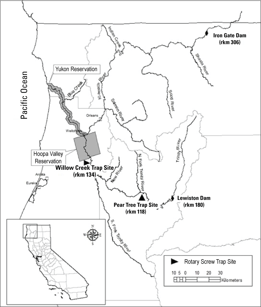
Trinity River and locations of major tributaries, dams, and the Pear Tree and Willow Creek fish traps. The restoration reach extends from Lewiston Dam to the confluence with the North Fork of the Trinity River, California.
Native anadromous fish of the Trinity River include Chinook salmon (Oncorhynchus tshawytscha), Coho salmon (O. kisutch), and steelhead trout (O. mykiss), all of which sustain valuable Tribal, commercial, and recreational fisheries (Trinity River Restoration Program and ESSA Technologies, Ltd., 2009). The Trinity Fish Hatchery, at the base of Lewiston Dam, has supplemented these fish populations to mitigate the loss of upstream fish habitat since 1958 (when dam construction began). Coho salmon belong to the Southern Oregon/Northern California Coast (SONCC) evolutionary significant unit (ESU), listed as threatened since 2005 under the federal Endangered Species Act (U.S. Department of Interior, 2000). Trinity River Chinook salmon belong to the Chinook salmon SONCC ESU, and in 1999 a petition for federal Endangered Species Act listing was declined.
The Chinook salmon population is comprised of two distinct subpopulations: spring and fall run. Adult spring Chinook salmon return to the Trinity River from April to September, and by July are concentrated in deep cold-water pools near Lewiston Dam. spring-run fish typically remain in cold-water refugia near the dam for months prior to spawning, which occurs from late September through October. Adult fall Chinook salmon return to the Trinity River from August to December and hold for shorter periods of time prior to spawning. Spawn timing for fall-run fish typically begins in mid-October, peaks in November, and ends in late December. Spawning activity is concentrated near Lewiston Dam early in the spawning season, and then diffuses throughout the river as the season progresses.
Since 2000, the TRRP has worked to improve and restore fish habitat and to promote fluvial geomorphic processes in the restoration reach of river that spans from Lewiston Dam downstream to the confluence with the North Fork Trinity River. This section of river also defines the spatial extent for the current application of S3 for the Trinity River. Fish populations in the restoration reach are monitored intensively. Spawner surveys are performed annually to estimate spawner abundance (Chamberlain and others, 2012). Juvenile production is monitored using mark-recapture methods at rotary screw traps fished at Pear Tree Gulch and Willow Creek (Petros and others, 2017).
Methods
First, we present methods for construction of the habitat template, the extrapolation of capacity-flow relations to unmeasured habitat units, and development of the physical and biological inputs used by S3. Next, we define a set of candidate models to test hypotheses about the mechanism by which density dependence affects population dynamics. Last, we describe methods for model calibration and parameter estimation, along with the model selection criteria we use to identify which candidate model best fits observed abundance estimates.
S3. Model Inputs
Habitat Template
The spatial domain of the S3 model is defined by a one-dimensional series of discrete habitat units. Habitat units are spatially referenced by their upstream and downstream boundaries measured as the distance in river kilometers from the confluence of the Trinity and Klamath rivers. The length of a habitat unit is simply the difference between its upstream and downstream boundaries. Habitat unit boundaries were defined by a combination of field surveys and Geographic Information System (GIS) mapping. To define the MHU boundaries for the Trinity River, field biologists delineated MHUs at transitions between three distinct meso-habitat types: riffles, runs, and pools. The Trinity River S3 model totals 910 habitat units between Lewiston Dam and its confluence with the Klamath River, of which 356 MHUs lie within the restoration reach (fig. 1). MHU delineations were drawn perpendicular and normal to the river flow using orthographic satellite imagery and GIS.
Habitat Capacity
To define the quality and quantity of fish habitat within each MHU we used habitat models developed for the restoration reach (Som and others, 2018a; Perry and others, 2018a) applied to the cells of 2-dimensional (2D) hydraulic models for the restoration reach (Bradley, 2018) and segments of the lower Trinity River (Som and others, 2018b). For this application, we assigned cells of the finer-scale hydraulic model to each MHU. We used the habitat model of Som and others (2018a), following the methods of Perry and others (2018a), to calculate the carrying capacity of each cell of the 2D hydraulic model over a range of river flows. The total carrying capacity of each MHU was then calculated by summing the capacity of each cell within an MHU to construct the one-dimensional inputs required by the S3 model.
Of the 910 meso-habitat units in the Trinity River S3 model, 380 were modeled using the 2D hydraulic models, leaving 530 unmodeled habitat units that fell outside the domain of the 2D models. To estimate flow-to-capacity relations for the unmodeled MHUs, we used an extrapolation technique similar to that used on the Klamath River (Perry and others, 2018c). However, we extended the extrapolation procedure to include a bootstrap sampling procedure to estimate uncertainty associated with the extrapolation procedure.
Habitat capacity for juvenile Chinook salmon fry and parr were extrapolated using 356 source habitat units from the restoration reach and 24 source habitat units from the lower Trinity River. The flow-to-capacity curves for these MHUs were used as “source” habitat units, with different flow-habitat relations, which were applied to the 530 unmeasured “target” habitat units downriver of the restoration reach. The habitat unit library is hierarchical, so that the measured habitat units were assigned to one or more of six general reach types. Within each of these reach designations the habitat units were also categorized by habitat type: “Run,” “Riffle,” or “Pool.” Unmeasured target habitat units were assigned to one of the six combinations comprised of six source reaches from the measured habitat units. Likewise, habitat units were matched according to similar channel morphology and then habitat type. Matching source to target reaches was done via deliberations between personnel from the Yurok Tribe and the USFWS that were familiar with the Trinity River and its fluvial morphology. Matching source reaches to target reach types in the lower Trinity River ensured that flow-to-habitat relations of unmeasured units would be drawn from source reaches with similar morphological structure. The source reaches (and river kilometer range relative to Klamath River confluence) with modeled hydrodynamics were: (1) Willow Creek (rkm 34–37), (2) Prairie Creek (rkm 97–117), (3) Junction City (rkm 117–129), (4) upper Junction City (rkm 129–139), (5) canyon (rkm 140–147), and (6) Limekiln (rkm 157–165). These six reach designations were then used in six different combinations to designate the source samples to be mapped to the unmeasured target habitats within the lower Trinity River. For example,
-
• 247 target habitat units were mapped to similar habitat units within source reaches 2, 5, and 6;
-
• 92 target habitat units were mapped to similar habitat units within source reaches 2, 4, 5, and 6;
-
• 1 target habitat unit was mapped to similar habitat units in reach 2;
-
• 19 target habitat units were mapped to similar habitat units within source reaches 1,2, 5, and 6;
-
• 111 target habitat units were mapped to similar habitat units within source reaches 1 and 3; and
-
• 60 target habitat units were mapped to similar habitat units within source reaches 1 and 5.
The capacity curves from the 2D models could not be applied directly to the unmodeled habitat units in S3 because target units will have a different length, width, and range of flows than the source habitat units, especially if tributaries enter between source and target units. Thus, the capacity curves had to be scaled proportionately from source to target units. Our procedure for scaling capacity curves scaled carrying capacity according to expected length and width differences between source and target unit. We used the following steps to extrapolate capacity area from source to target units:
-
1. Standardize capacity for each source unit by dividing by the length of the habitat unit, which yields capacity per linear meter of stream (m2/m).
-
2. Calculate the exceedance probability associated with a given daily river flow for each target habitat unit.
-
3. Quantify the relation between channel width and river flow (using output for the habitat units from the 2D hydrodynamic models), where channel width was calculated as the total wetted surface area divided by the channel length. This relation is calculated over a range of common exceedance probabilities.
-
4. Use the flow-to-width relation for each exceedance probability from step 3 to estimate mean channel width of each target unit at a given daily river flow.
-
5. Use the flow-to-width relation to estimate the mean channel width of the source unit associated with the same exceedance probability of the target habitat unit in step 4.
-
6. Scale the capacity (K, see Juvenile Capacity section) using the average width of the target unit relative to the source unit by multiplying K by the ratio of source to target channel widths:
Our procedure for scaling capacity curves over the range of flows is based on established continuity equations that define hydraulic channel geometry as a power function of discharge (Leopold and Maddock, 1953). Leopold and Maddock (1953) showed that geometric channel properties (such as channel width) along a river’s longitudinal profile follow a power function at common exceedance flows:
whereis the width of habitat unit h,
is the discharge of the habitat unit associated with exceedance probability p, and
and
are parameters that vary with exceedance probability.
To develop the width continuity equations for S3, we first quantified exceedance flows in 1 percent increments for all 910 habitat units using a 39-year historical flow record provided by Perry and others (2011) and Jones and others (2016). Second, for all 2D habitat units, we (1) estimated mean channel width as the wetted surface area divided by the length of the habitat unit, and (2) averaged the width of replicate habitat units at a given 2D site to develop composite widths associated with each source capacity curve. Third, we estimated the parameters of equation 2 by fitting log-log linear regressions to the widths of all habitat units at flows associated with each 1 percent increment of exceedance (fig. 2).
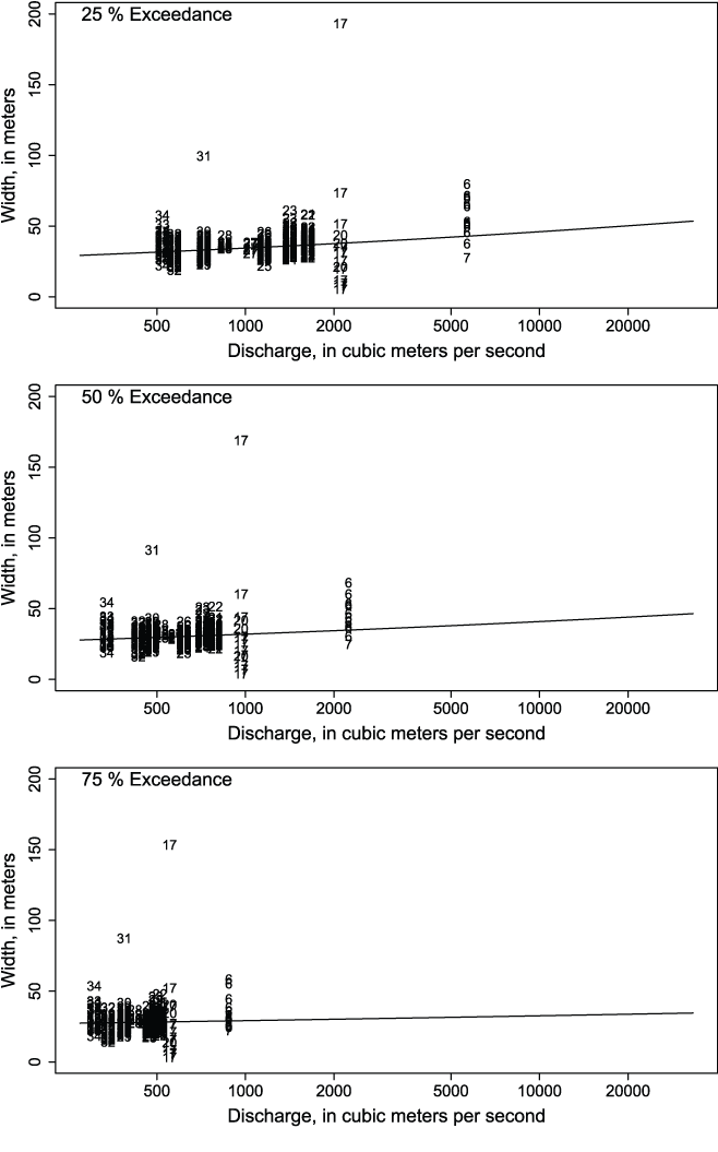
The relation between discharge and channel width of habitat units at 2D sites for selected exceedance probabilities. Symbols represent the 34 hydrologic reaches that were output via the River Basin Model-10 to obtain flows for the Trinity River, California.
These equations served two functions: (1) they let us scale discharge between source and target habitat units by relating flows at different locations to common exceedance probabilities, and (2) they provided an estimate of channel width of both source and target unit at a common exceedance probability, which allowed us to scale capacity by the relative change in channel width between source and target unit.
Once the source reaches and units were assigned to reaches and units of the lower Trinity River, we used a bootstrap approach by drawing random samples with replacement to assign source habitat units to unmeasured target habitat units. Habitat types were assigned using a stratified random sample with run, riffle, and pool habitat types forming the strata. For example, pools from a given reach type library were randomly selected to assigned pools in the target habitat units of the same reach type. We conducted 100 stratified bootstrapped samples of randomly chosen habitat units for a given reach type and habitat type. Because only the reach types were chosen through group consensus, we felt this hierarchical bootstrap approach was more objective than arbitrarily mapping a target habitat unit to a source habitat unit.
Bootstrapped estimates of capacity for target habitat units reflected the relative differences in capacity among the habitat types but estimates of capacity differed between source and target habitat units (table 1 and fig. 3). Distributions of juvenile Chinook salmon capacity by habitat type (fry or parr per m2) at flows from 274 to 5,000 ft3/s were right-skewed and highly variable as a result of geomorphic differences among habitat types over a wide range of flows. For source habitat units, the 2.5 percentile for fry capacity was 19.1 fry/m2, the median was 55.1 fry/m2, and the 97.5 percentile was 155.2 fry/m2. Similarly, the 2.5 percentile for parr capacity for target habitat units was 3.7 parr/m2, the median was 16.7 parr/m2, and the 97.5 percentile was 465.7 parr/m2. For target habitat units, the 2.5 percentile for fry capacity was 7.8 fry/m2, the median was 44.8 fry/m2, and the 97.5 percentile was 228.2 fry/m2. Similarly, the 2.5 percentile for parr capacity for target habitat units was 1.9 parr/m2, the median was 16.8 parr/m2, and the 97.5 percentile was 423.3 parr/m2. Overall, the distribution and median capacity was similar between those bootstrapped for target habitat units and measured source habitat units, whereby some habitat units have little constraint on capacity (>400 fry or parr per m2), especially at high flows. Therefore, for use in S3, we used the median capacity for each habitat unit across the bootstrap samples at a given flow as the capacity of an unmeasured unit at a given flow.
Table 1.
Summary statistics for useable spawning area, in square meters (m2), and the capacity of fry and parr per m2 for source and target habitat units.[Abbreviations: Min, minimum; Max, maximum. Symbols: %, percent; >, greater than.]
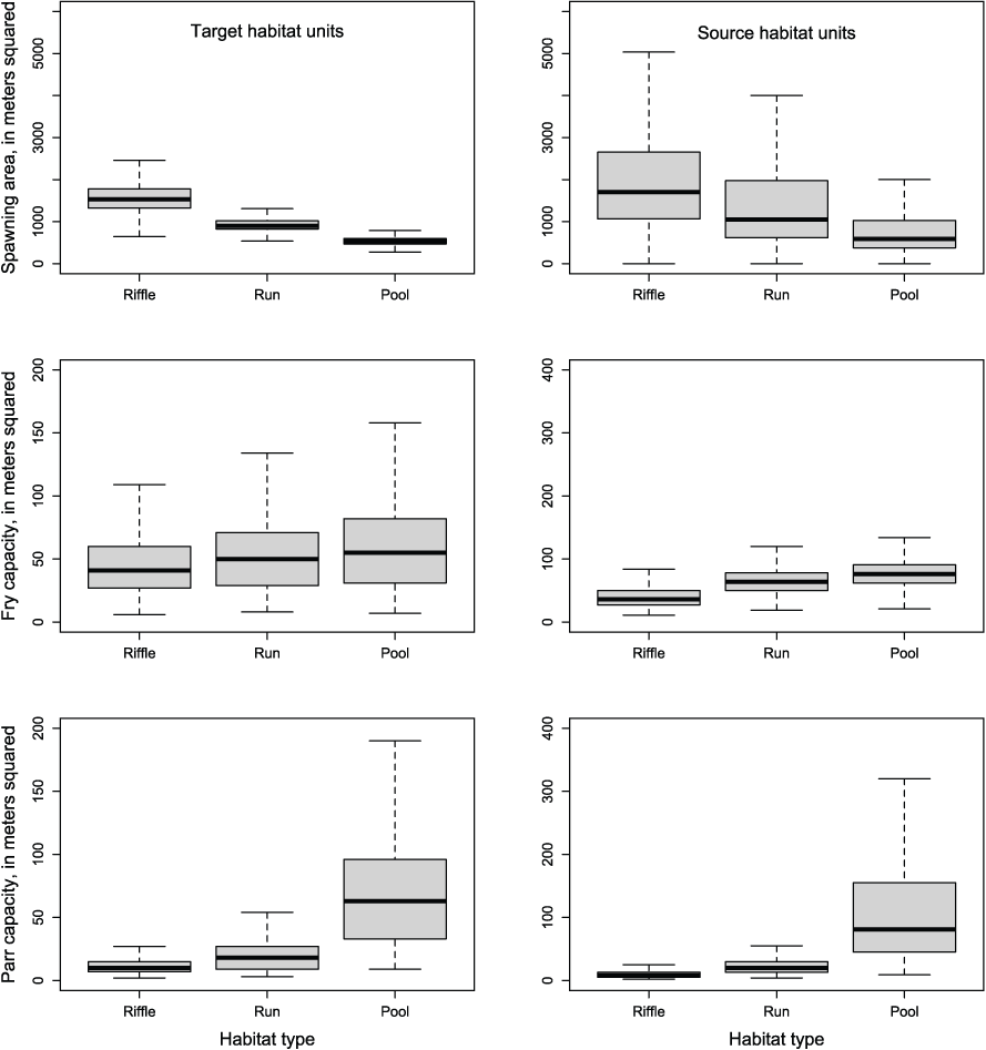
The distribution of capacity estimates for individual habitat units by habitat type and source versus target habitat units over river flows from 274 to 5,000 cubic feet per second. The median is thick line, the quartiles are the extent of the boxes, the whiskers represent 1.5 times the interquartile range. Definitions for habitat type are based on characteristics at base flows such that a pool at base flow may have characteristics of a run at higher flow.
Physical Inputs
The S3 model requires two physical inputs that drive population dynamics, either directly or indirectly: (1) water temperature and (2) streamflow. The S3 model requires these inputs as a timeseries of daily mean water temperature (degrees Celsius [°C]) and daily mean discharge (cubic feet per second [ft3/s]) for each MHU. We used RBM10 (Jones and others, 2016) to simulate the historical timeseries of temperature and stream flow for the restoration reach and the lower Trinity River below the Pear Tree trap. Daily mean temperature and daily mean stream flow were output for locations 0.32 rkm downstream from Lewiston Dam and 0.32 rkm downstream from seven main-stem tributaries included in the RBM10 model (table 2). These 33 output locations accounted for flow accretions and the associated changes in water temperature. RBM10 output was mapped to each MHU in S3 such that flow and temperature were constant among MHUs between tributaries but varied among reaches between tributaries (table 1).
Table 2.
Tributaries included in the River Basin Model-10 (RBM10) water temperature model that lie within the Trinity River restoration reach, RBM10 output locations, and the corresponding Stream Salmonid Simulator meso-habitat units associated with the RBM10 output.[Abbreviations: Cr., Creek; R., River; rkm, river kilometer; Stn., Station]
Biological Inputs
The S3 model relies on the three primary forms of biological inputs to simulate population dynamics: (1) female spawners, (2) juvenile hatchery fish releases, and (3) juveniles entering from tributaries.
Female Spawners
To develop inputs for the number of female spawners, spawner survey data (Chamberlain and others, 2012) were summarized as a weekly time series of redd counts by survey reach. Of the 14 spawner-survey reaches between Lewiston Dam and the Klamath River confluence, seven reaches fall within the restoration reach (table 3). We modeled two distinct spawning subpopulations in S3, early and late spawners, which track the timing of spawning for spring and fall Chinook salmon. Because spring and fall Chinook salmon redds cannot be visually differentiated, the State of California’s Department of Fish and Wildlife (CDFW) estimates a spawning cut-off date that determines when redds switch classification from spring Chinook salmon to fall Chinook salmon. CDFW generates this cut-off date based on coded-wire tag recoveries collected at the hatchery (Borok and others, 2015). To assign spawners to subpopulations in S3, we adopted the cut-off dates provided by CDFW. Although we label the early and late-spawning populations as “spring” and “fall” Chinook salmon in this report, we recognize that a simple cut-off date does not capture overlap in the temporal spawning distribution of spring and fall Chinook salmon. Furthermore, the cutoff date based on hatchery returns may not be representative of the timing of in-river spawning. Therefore, although we label the modeled populations as “spring” and “fall,” the reader is advised to recognize that the S3 model is tracking the progeny of these early (spring) and late (fall) spawners based on the cutoff date provided by CDFW.
To construct model inputs, we mapped the reach-level redd survey data to each MHU and converted the weekly counts of female spawners to daily counts by dividing weekly counts by seven (table 3). Within each survey reach, daily number of female spawners were then distributed to MHUs proportional to the distribution of daily redd capacity in each survey reach.
Table 3.
Location of spawning survey reaches for the Trinity River that were used as input for the number of spawners that are allocated to each habitat unit in Stream Salmonid Simulator.[Abbreviations: km, kilometer; rkm, riverkilometer]
Female Spawners in the Lower Trinity River and Tributaries
The data collected on the spawning population to estimate the number of female spawners provide a robust estimate for the restoration reach of the Trinity River. However, there is little information on the spawning population in the lower Trinity River below rkm 77.6. We assumed a proportion of female spawners = 0.5 for years where sex ratios were unavailable, which was approximately the average sex ratio from 2005 to 2010. The product of the proportion of female spawners and the total run reported in the Klamath/Trinity Basin MegaTables for the years 2005–17 (Klamath/Trinity Basin Megatables, 2022) provided the total annual number of females entering the Trinity River. We estimated the annual number of females available to spawn in the lower Trinity River (table 4) by subtracting the total annual number of female spawners estimated from carcass mark-recapture surveys in the upper Trinity River (spawning reaches 1–10; table 3) from the total number of spawners in the MegaTable.
Table 4.
Annual number of fall and spring Chinook salmon (Oncorhynchus tshawytscha) female spawners that were used as inputs to the Stream Salmonid Simulator model, Trinity River, California.[Annual numbers based on subtracting the estimates within the restoration reach of the Trinity River (spawning reaches 1–7; table 2) from the total number of females entering Trinity River, California.]
To estimate the number of adult female Chinook salmon that spawned in the lower Trinity River, versus those that spawned in tributaries, we took the total watershed area of the lower Trinity River and four major tributaries and then calculated the proportional area among these five river segments. The major tributaries considered (and their percent area) were: (1) Canyon Creek (64 mi2; 2.2%), (2) North Fork of the Trinity River (152.4 mi2; 5.3%), (3) the New River (233.6 mi2; 8.1%), and (4) the South Fork of the Trinity River (932.1 mi2; 9.2%). The lower Trinity was estimated at 2,969.8 mi2; representing 52.3 percent of the watershed area considered. Thus, subtracting the number of spawners in the survey data (spawning reaches 1–10; table 2) from the total number of female spawners in the MegaTable provided the total number of female spawners to be partitioned among the tributaries and lower Trinity River (tables 4 and 5). These annual numbers of fish were allocated to a tributary or river based on their proportional watershed area. Allocating the number of spawners according to watershed area is supported by studies that demonstrate fish production as a function of watershed size (Liermann and others, 2010). The adult female spawners allocated to the different tributaries (table 5) allowed us to estimate the number of juvenile salmon entering from the tributaries and be used as input for S3 simulations.
Table 5.
Annual number of fall and spring Chinook salmon (Oncorhynchus tshawytscha) female spawners that were allocated to each of the four tributaries of the Trinity River, California.[Annual numbers based on the proportion of water shed area relative to the total watershed area. These adult spawners provided the number of juvenile salmon entering from the tributaries to be used as Stream Salmonid Simulator inputs. Abbreviations: Canyon, Canyon Creek; New, New River; NF, North Fork Trinity River; SF, South Fork Trinity River]
Juvenile Salmon Entering from the Tributaries and Hatchery
To calculate the number of juvenile Spring and fall Chinook salmon entering from the tributaries, we used data from Klamath River tributaries to develop a relation between watershed area and the number of juvenile salmon recruits per adult female spawner (Hendrix and others, 2011). Specifically, we used the annual stock-recruitment data (1993–2008) obtained for four Klamath River tributaries: Bogus Creek, the Shasta River, Scott River, and the Trinity River to develop a power equation between watershed area (mi2; ) and annual estimates of the number of recruits per spawner, which yielded the following equation:
where the intercept, =8.1107 (SE=0.9176) and the slope for watershed area,=-0.5276 (SE=0.1392; r2=0.269.) estimate the expected annual production of juveniles per female spawner (RST) for the given tributary’s corresponding watershed area (AwT). The product between the annual number of female spawners (S) and the expected number of juvenile recruits per spawner (RS) provided the estimate of the total annual number of juvenile recruits that survived and emigrated from a tributary to the Trinity River (JTy; table 5) such that:Because the S3 model also requires the entry timing of tributary-sourced juvenile Chinook salmon into the Trinity River, we first estimated the mean week of out-migration using the relation between the number of recruits per spawner and the mean calendar week of out-migration obtained from the fish trap data on the four Klamath River tributaries mentioned above. The mean week of outmigration for Trinity River tributaries was fit to annual (y) data from Klamath River tributaries (T) and it can be expressed as:
where When fitting this equation to the data =3.723 (SE=0.121) =-0.173 (SE=0.025), and r2=0.556. To apply this equation to Trinity River tributaries, we used RST for each tributary to estimate the mean weekly outmigration. We then assumed a normal distribution for the expected W for each tributary to determine the proportion of the total annual juvenile production (eq. 3) from each tributary that would be expected to out-migrate in weeks earlier and later than the mean outmigration week, thereby providing an estimate of the expected weekly number of juveniles emigrating from each tributary and year.The last key input that must be estimated for juvenile salmon entering from the tributaries is the mean weekly size of the fish upon entry into the main-stem Trinity River. To estimate the weekly size of juveniles emigrating from tributaries, we regressed the mean lengths of juvenile fish obtained from the Klamath River tributaries at fish monitoring traps (including the Trinity River) against the mean week of their out-migration using the following equation:
whereis the mean weekly fork length (FL; mm) given the week of outmigration observed across years and tributaries of the Klamath River.
Trinity River Hatchery released two to three times as many juvenile fall Chinook salmon as spring Chinook salmon, depending on the year (table 6). Annual releases of juvenile spring Chinook salmon ranged from 662,000 to 948,000, whereas releases of fall Chinook salmon ranged from 1.8 to 2 million. Based on the mean size of release groups, there was considerable variation among years in the life stage at which spring Chinook salmon were released. In two of the years, only smolts were released; in two other years, only parr were released; and in one year, about 60 percent more parr than smolts were released. In contrast, for fall Chinook salmon, hatchery releases were comprised of parr exclusively for all years used in calibration
Table 6.
Estimated annual number of juvenile fall- and spring-run Chinook salmon (Oncorhynchus tshawytscha) entering from tributaries and the Trinity River Hatchery, California.[Estimates for the tributaries are based on the production of juveniles as a function of total watershed area and the total number of spawners to the tributary. Abbreviations: Fall, late fall; Spring; early spring]
Stream Salmonid Simulator Submodels and User-Defined Parameter Settings
When simulating fish populations with S3, some population dynamics are dictated via user defined options and parameter inputs. Juvenile fish populations in the S3 model are affected by three dynamic processes: (1) survival, (2) growth, and (3) movement. We describe how the submodels were parameterized for the Trinity River and specify values of user-defined parameters. For details on the mathematical structure of individual submodels, see Perry and others (2018b). The biological processes of survival, growth, and movement are determined by life stage, which in S3 are (1) spawning, (2) egg development, and the juvenile life stages of (3) fry, (4) parr, and (5) smolt. Other than updates based on more data availability, we used the same set of assumed parameters and data when originally calibrating the model to the weekly abundance estimates at the Pear Tree trap site (Perry and others 2018a).
Spawning, Egg Development, and Egg Survival Submodels
The number of eggs that survive to emerge as fry is affected by several S3 parameters and submodels. We set the fecundity of female spawners to 3,046 eggs per redd to approximate the mean number of eggs observed for Chinook salmon returning to the Trinity River Hatchery from 2000 to 2017. The mean time from spawning to fry emergence is modeled as a function of daily water temperature and accumulation of degree days (see Perry and others, 2018b). Variation in emergence timing is assumed to follow a normal distribution about the mean emergence date and is controlled by the standard deviation in degree days required to hatch, which we set to 26.6 °C days (Perry and others, 2018b).
During the incubation period, S3 considers three mechanisms that affect egg-to-fry survival: (1) baseline “natural” mortality, (2) temperature-related mortality, and (3) redd superimposition (Perry and others, 2018b). The natural mortality rate was set at 0.25 percent per day, which equates to a baseline survival rate of about 92.8 percent per month. Thermal tolerance parameters were set so that water temperatures less than or equal to 17 °C had no effect on egg survival, but temperatures greater than 17 °C imposed a daily mortality rate of 25 percent (Geist and others, 2006).
Redd superimposition is the process whereby a later arriving spawner builds a redd on top of an existing redd and dislodges or entombs the eggs laid by the earlier spawner. Superimposition is modeled in S3 as a function of habitat capacity and spawner abundance. The probability of redd superimposition is defined by redd density (redd abundance/redd capacity), which is calculated and applied daily for each MHU. The amount of redd mortality attributed to superimposition on day t is simply the number of redds to be recruited that day multiplied by the existing pre-recruitment redd density. However, given the propensity of Chinook salmon to guard their redds until death, the S3 model allows the user to set a “guarding period” parameter. We set the guarding period to 10 days, assuming semelparous Chinook salmon live to guard their nests for 10 days after spawning. Redds are not vulnerable to superimposition during the guarding period.
Although redd-scour owing to freshets is known to influence the survival of eggs, we have not yet implemented mortality owing to scour in the Trinity River S3 model, because there is little evidence for substantial redd scour in brood years we used for calibration. Incorporating the effects of sediment load and redd scour sufficiently into S3 simulations is an area of ongoing interest. The S3 model team and collaborators are seeking ways to include a function that can tenably account for the effects of egg-scour on redd survival.
Juvenile Growth
S3 provides two options for temperature-driven growth models: the Ratkowsky Model and the Wisconsin Bioenergetics Model (Perry and others, 2018b). Mean fish size for each source population and life stage in each habitat unit was incremented daily as a function of water temperature using the Wisconsin Bioenergetics Model with a revised consumption function (Plumb and Moffitt, 2015). For application to the Trinity River, we fixed the proportion of maximum consumption parameter to 0.66 and set all other parameter values to those listed in Perry and others (2018b). Under this parameterization, the Wisconsin and Ratkowsky growth models show similar growth rates over a range of water temperatures (Perry and others, 2018b). The growth model governs life-stage transitions by moving fish to the next life stage when their mean size exceeds user-defined size thresholds for each life stage. For our simulations, the juvenile life-stage classifications were fry: fork length (FL) ≤ 50 millimeters (mm); parr: 50 < FL ≤ 90 mm; and smolt: FL > 90 mm. For natural-origin fish, we set the weight of emergent fry to 0.3 grams, which back-calculates to a fork length of 30 mm (see app. 1–4). The mean size of fry, parr, and smolt were recomputed daily within each MHU to account for daily growth, growth-based life-stage transitions, recruitment of emergent fry, and movement among habitat units. We assumed that the growth model applied uniformly to all juvenile life stages, natural- and hatchery-origin fish, and spring and fall Chinook salmon subpopulations.
Juvenile Movement
S3 has two submodels for simulating fish movement: (1) the “mover-stayer” model, and (2) the “advection-diffusion” model (Perry and others, 2018b). In both models, movement from one MHU to another is simulated in the downstream direction only. In our simulations, we used the mover-stayer model for rearing fry and parr, and the advection-diffusion model for actively migrating smolts. The mover-stayer model can be implemented with density-independent or density-dependent movement, which is a user-specified option. With density-independent movement, abundance and capacity have no effect on movement probability. Density-independent movement is the only option available with the advection-diffusion model.
Two parameters drive movement in the mover-stayer model: (1) the probability of remaining in the currently occupied MHU (Pstay) from time t to t+1 (resulting in “stayers”), and (2) the mean distance moved downstream (that is, resulting in “movers”; kilometers per day). For the density-dependent form of the model, Pstay is expressed as a Beverton-Holt function such that Pstay declines as the ratio of abundance to capacity increases. That is, the probability of moving (1-Pstay) increases as abundance approaches capacity. We estimated the Pstay parameter for density-dependent and density-independent forms of the mover-stayer model. The mean distance moved was calculated deterministically as a function of fork-length, using the same size-based movement rate as we used for the smolt life stage, as described in Perry and others (2018a, b).
We modeled smolt movement using a density-independent advection-diffusion process because this model was developed for actively migrating smolts, not smaller rearing fish that are less likely to move downstream (Zabel and Anderson, 1997; Zabel, 2002). The advection-diffusion model assumes that the spatial distribution of a population at a given point in space after t time units is described by a normal distribution with a mean location and standard deviation. We allow the movement rate of smolts to depend on size, with the rate of movement increasing with fish size. The parameters of this model were based on size relations developed by Zabel (2002) and Plumb (2012) for juvenile Snake River fall Chinook salmon (Perry and others, 2018b).
Juvenile Survival
Daily survival probability, like movement probability, can be specified either as density-independent or density-dependent. In the density-dependent form, survival probability is expressed as a Beverton-Holt function that decreases as the ratio of abundance to capacity increases (Perry and others, 2018b). In this form, we estimate the expected survival as abundance approaches zero. In the density-independent form, daily survival probability is estimated as a constant value that does not depend on abundance or habitat capacity. Under both forms of the survival model, parameters may be allowed to differ among life stages and source-populations. Parameters of the survival model were estimated via calibration. We compare alternative models that use either the density-independent or density-dependent form of the survival model. Additionally, we allow the parameters to vary among life stages and source populations.
Model Calibration
Juvenile Abundance Data
We calibrated S3 to 13 years of weekly juvenile Chinook salmon abundance estimates from the Pear Tree and Willow Creek fish traps. We calibrated to abundance estimates from brood years 2005–17. These years were selected based on the completeness and robustness of the juvenile abundance estimates among available years. For all years, we fit S3 to 694-point estimates at the Pear Tree trap and 665-point estimates at the Willow Creek trap that represented weekly abundance of juvenile Chinook salmon passing the traps. Weekly abundance estimates were separated into hatchery and natural origin but were not otherwise broken down by life stage or tributary source. We used the calibrated model to simulate abundance of fish passing a trap and then compared simulated to observed weekly abundances in similar manner as Perry and others (2018a, c) for each trap separately.
Calibration
The goal of calibration was to estimate survival and movement parameters of the S3 model by fitting the model to estimates of weekly abundance of juveniles passing the Pear Tree and Willow Creek fish traps. To fit the model to abundance estimates, we used a likelihood function where deviations between simulated and estimated weekly abundances followed a normal distribution:
whereis the number of juveniles estimated to have passed the trap in week w of year y,
is the simulated number of juvenile salmon passing the trap in week w of year y for a given vector of parameters , and
is a normally distributed error term with mean zero and standard deviation σ.
is the negative log-likelihood of the parameters given the observed data and specified model structure, and
ww,y
are weights that are proportional to the uncertainty in each .
Although the S3 model simulates daily abundance by life stage and source population, weekly abundance estimates () were aggregated over all life stages but were separated for natural- and hatchery-origin fish. Consequently, for fitting the model to observed data, represents the total simulated weekly abundance passing a trap, summed over life stages and source populations separately for natural- and hatchery-origin juveniles.
Given a fitted model, we used a parametric bootstrap routine to generate confidence intervals in simulated weekly abundance of fish passing the traps. First, we generated 100 parameter sets by drawing each parameter set from a multivariate normal distribution with the mean parameter vector and variance-covariance matrix estimated through model calibration. Next, we ran S3 for each of the parameter sets and summarized the weekly abundance passing each trap. Last, bootstrap confidence intervals for each simulated weekly abundance were generated using the 2.5th and 97.5th percentile of the output from the 100 model runs.
Model Selection
To determine which formulation of the survival and movement parameters best explain the dynamics of the juvenile Chinook salmon outmigration, we fit a set of four candidate models to the weekly abundances at the Pear Tree trap and the Willow Creek trap. We fit each candidate model separately to each trap to understand how parameter estimates differed across different datasets and different model domains. When fitting to the Pear Tree trap, parameters represent average survival and movement within the restoration reach where there were data on spatiotemporal spawner abundance, a hydrodynamic model with which to estimate capacity for every mesohabitat unit, and no major tributaries contributing juveniles to the main stem. In contrast, when fitting to the Willow Creek trap we assumed the spatiotemporal distribution of spawners, approximated the numbers of juveniles entering from tributaries, and extrapolated the meso-habitat units with capacity relations.
The four candidate models represented different combinations of density-independent or density-dependent survival or movement: (1) density-independent survival and movement, (2) density-independent survival and density-dependent movement, (3) density-dependent survival and density-independent movement, and (4) density-dependent survival and movement (table 7). By fitting different combinations of density-dependent movement and survival models to the same dataset, we compared the fit of the different candidate models to the data and evaluated which combination best explained the weekly abundances of fish passing the trap.
We assumed a priori that movement and survival parameters differed by life stage and among hatchery and natural-origin populations, yielding six estimated parameters for each model (table 7). Each model estimated three movement parameters and three survival parameters. For movement, we estimated a unique Pstay for natural-origin fry and parr. We also estimated a unique Pstay parameter that was common for both hatchery-origin fry and parr because the vast majority of hatchery releases were of parr size, and there was not enough data on hatchery fry to estimate unique parameters for each life stage. Movement parameters of both natural- and hatchery-origin smolts were fixed according to the advection-diffusion model described in Perry and others (2018b). For survival, unique parameters were estimated for natural-origin fry. However, we estimated common survival parameters for parr and smolt life stages because there was not enough information in the trapping data to estimate unique survival parameters for these life stages. A third common survival parameter was estimated for hatchery-origin fry, parr, and smolt because the calibration routine had difficulty estimating unique survival parameters of hatchery-origin fish by life stage.
We compared the relative rank of each candidate model using Akaike information criterion (AIC), where the lowest AIC value indicates the model with the most support given its fit to the data and the number of parameters (see Burnham and Anderson, 2002). In this model selection framework, the best model has the lowest AIC score, and models within two AIC points are deemed competitive alternatives.
Table 7.
Candidate Stream Salmonid Simulator models that were fit to weekly estimated abundances at the Pear Tree and Willow Creek traps on the Trinity River, California.[Model: S, survival; M, movement; I, density-independent; D, the density-dependent model forms; g, indicating a group-effect for different source-populations (natural or hatchery origin); a, life-stage effect for different juvenile life stages (fry, parr, and smolt); *, a parameter relation between the group- and age-effects that allows life-stage specific parameters to differ among hatchery- and natural-origin fish populations]
Results
Calibration, Model Selection, and Parameter Estimates
Calibration
Fitting a complex simulation model like S3 to abundance data collected at fish traps is challenging because of the run time for the optimization of model parameters. For example, all but one model took more than 45 days to converge to the minimum log-likelihood when fitting the model’s parameters to the data. Model 2 fit to data from the Willow Creek trap did not converge to a minimum log-likelihood. As more of the river is included in the S3 model, the number of source populations and meso-habitat units in S3 increases, causing slower run times and longer times per iteration in the optimization routine. Slower run times are apparent when comparing the range of iterations obtained over the same period between the Pear Tree and Willow Creek traps. Considering the long run times and difficulty of fitting these models, improving the efficiency and statistical rigor of the fitting of model parameters would be beneficial.
Model Selection
Despite the differences in the underlying model structure between the trap sites, we obtained similar relative importance of density dependence on both survival and movement. Regardless of the trap site and data that we fit the S3 model to, models that expressed survival as a function of density-dependence were most supported by AIC model selection, and contrastingly the model where both survival and movement were density-independent were least favored (table 8). We obtained slightly different model selection results depending on the data from each of the fish traps. When fitting to the Pear Tree trap data, the fully density-dependent model for survival and movement (model 4; table 7) was the AIC best model, whereas the density-dependent survival model (model 3) was the AIC best model when fitting to data from the Willow Creek trap site.
Comparison of AIC values among the candidate models revealed differences in model fit to the weekly abundance estimates (table 8). For example, among the models fit to the weekly trap abundances at the Pear Tree trap site, models 2 and 3 were both similarly less than 2 AIC units from model 1 whereas models 2 and 3 were also greater than 7 AIC units from model 4 the AIC best model. These results support density-dependent processes affecting both movement and survival (model 4; fig. 4) because these models explained the abundances and run timing at the Pear Tree trap site. Similarly, models fit to the weekly abundances at the Willow Creek trap site also indicate that density-dependent survival and movement are relatively important factors in explaining variation in weekly abundances among the years.
![Graphs showing the convergence of candidate density-independent (I) and -dependent
(D) survival (S) and movement (M) models (models 1–4) plotted on the iteration number
when optimizing the model’s parameters to fit the modelled weekly abundances to the
weekly abundances at the Pear Tree (upper) and Willow Creek (lower) trap sites. [Cr.,
Creek]](https://pubs.usgs.gov/of/2023/1023/images/ofr20231023_fig04.png)
Graphs showing the convergence of candidate density-independent (I) and -dependent (D) survival (S) and movement (M) models (models 1–4) plotted on the iteration number when optimizing the model’s parameters to fit the modelled weekly abundances to the weekly abundances at the Pear Tree (upper) and Willow Creek (lower) trap sites. [Cr., Creek]
Table 8.
Model selection results and their corresponding parameter estimates for juvenile Chinook salmon (Oncorhynchus tshawytscha) survival and movement, Trinity River, California.[The candidate Stream Salmonid Simulator models were fit to weekly estimated abundances at the Pear Tree and Willow Creek traps on the Trinity River, California. Model: S, survival; M, movement; I, density-independent; D, the density-dependent model forms; for different source-populations (natural; W, or hatchery; H, origin); a, life-stage effect for different juvenile life stages (fry; f, parr; p, and smolt; s)]
Model fit when output from previous estimates (Perry and others, 2018a) were used against the current data.
Parameter Estimates
Daily survival estimates from fitting S3 to the weekly abundance estimates at the traps appeared relatively consistent across the models (fig. 5). However, small differences (> 0.005) in daily survival probability can have meaningful consequences due to the long-term probability of survival for a fish over a migration season (fig. 6). Likewise, there were marked differences in daily survival among the candidate models. Among models, we identified the biggest difference in survival and movement between hatchery and natural fish (figs. 5 and 6). Estimates of daily survival were lower for hatchery fish than for natural fish, and the daily holding probabilities for hatchery fish were consistently estimated at or near zero, indicating hatchery fish traveled faster and had a lower intercept in daily survival probability over the range in fish density than the natural fish in S3 fitting and simulations (fig. 7).
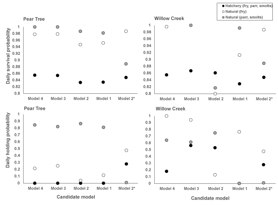
Parameter estimates from the candidate density-independent and -dependent survival and movement models (models 1–4; tables 6 and 7) fit to the Pear Tree and Willow Creek traps’ week abundance estimates for juvenile Chinook salmon (Oncorhynchus tshawytscha). Model 2* represents the parameter estimates reported by Perry and others (2018a).
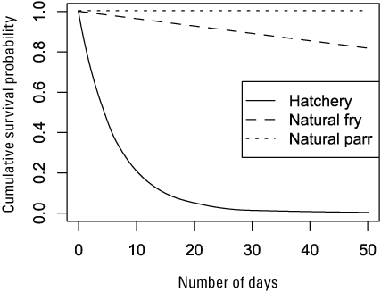
Graph showing the cumulative effect of time on survival probability for hatchery- and natural-produced subyearling Chinook salmon (Oncorhynchus tshawytscha) given a density of one fish. Parameter estimates for the intercept of the Beverton-Holt model (model 4) fit to the Willow Creek trap abundance estimates were used to produce the curves.
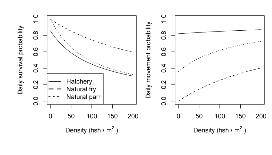
Graphs showing the effect of fish density on daily survival (left) and movement (right) probabilities for hatchery- and naturally produced subyearling Chinook salmon (Oncorhynchus tshawytscha). Parameter estimates for the intercept of the Beverton-Holt model (model 4) fit to the Willow Creek trap abundance estimates were used to produce the curves.
Simulated Versus Estimated Abundance
We evaluated how well simulated abundance at each trap compared to observed abundance when using parameters from the best fit model (model 4) fitted to Willow Creek trap data. Overall, the model predicted the weekly abundances of juvenile Chinook salmon at the fish traps poorly (fig. 8). Simulated abundances at both traps were often near zero when estimated abundances were higher, indicating that when S3 was fit to all years of data simultaneously, the resulting simulated weekly abundances were lower than weekly abundances measured from trap catches for both hatchery and natural juvenile Chinook salmon. At the Willow Creek trap, peak weekly abundances for the natural juvenile Chinook salmon were simulated lower than the estimated weekly abundances at the Willow Creek trap. Comparing simulated annual abundance to the total annual trap abundances provided a complementary picture to weekly values. Nonetheless, years that were particularly over or underestimated were more apparent when compared on an annual basis (fig. 9). The best fit to annual abundance of natural fish occurred when model parameters estimated from the Pear Tree trap were used to simulate abundance of fish passing the Willow Creek trap (figs. 2.3 and 2.4).
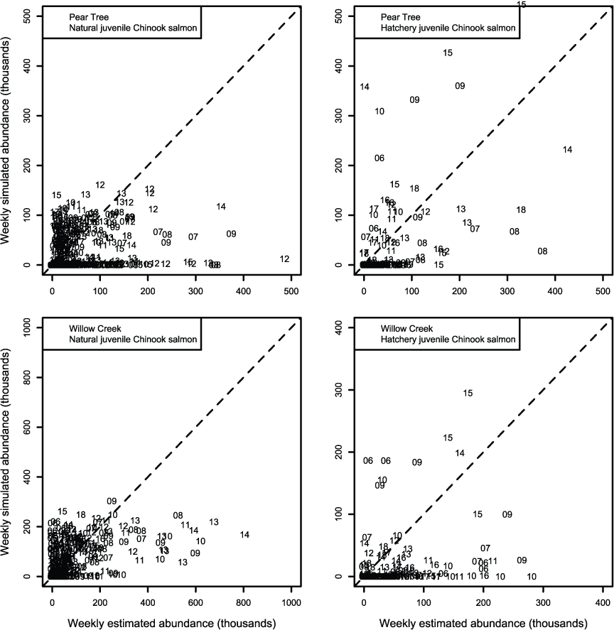
Weekly abundance estimates for Trinity River Chinook salmon (Oncorhynchus tshawytscha) that passed Pear Tree and Willow Creek fish traps compared to those simulated by the Stream Salmonid Simulator (S3) model under model 4 that was fit to the weekly abundances at the Willow Creek trap. Data points represent the last two digits of the juvenile out-migration year.
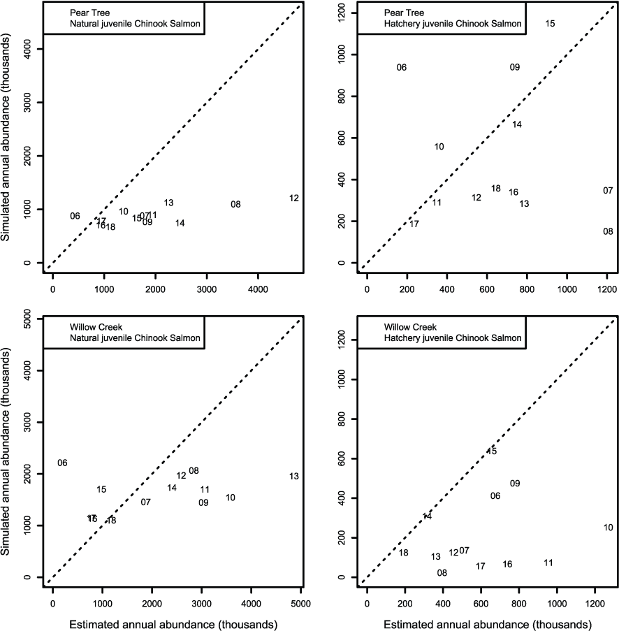
Graphs showing annual abundance estimates for juvenile Trinity River fall Chinook salmon (Oncorhynchus tshawytscha) that passed the Pear Tree and Willow Creek fish traps compared to those simulated by Stream Salmonid Simulator (S3) model. Data points represent the last two digits of the juvenile out-migration year.
Simulated and Estimated Migration Timing
Migration timing of juvenile Chinook salmon passing the Willow Creek fish trap was approximated by S3. Simulated migration timing tracked the inter-annual variation in the estimated 20th, 50th, and 80th percentiles very well over the 13 years of data (figs. 10 and 11), though a consistent earlier simulation of migration dates was apparent.
However, for the Pear Tree trap, the model consistently predicted later migration dates than those generated from weekly abundance estimates. At Pear Tree trap, the simulated 20th, 50th, and 80th percentiles in migration dates were generally later than the estimated migration timing. The discrepancy between simulated and estimated migration timing at the Pear Tree trap was especially apparent in 2015, 2016, and 2017 when weekly abundance estimates indicated a high abundance in January.
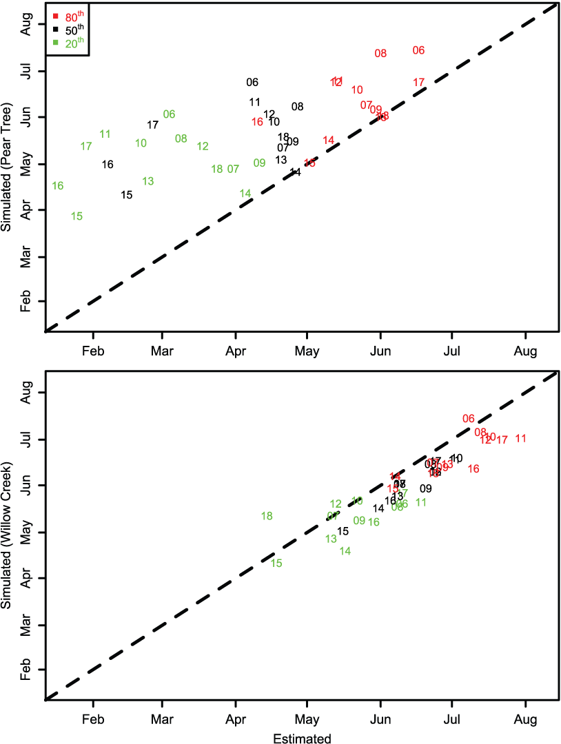
The 20th, 50th, and 80th percentiles in the annual migration dates for Trinity River juvenile Chinook salmon (Oncorhynchus tshawytscha) that passed the Pear Tree and Willow Creek fish traps versus those that were simulated by the Stream Salmonid Simulator model. Data points represent the last two digits of the migration year.
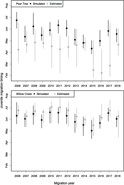
Range from the 20th to 80th percentiles (extent of bars) and the median (data points) in the annual migration dates for Trinity River Chinook salmon (Oncorhynchus tshawytscha) that passed the Pear Tree and Willow Creek fish traps and those simulated by the Stream Salmonid Simulator (S3) model.
Simulated and Observed Fish Size
Although we used a literature-based average value for p(Cmax), simulated mean fish length tracked the average seasonal trend in the size of fish passing the Pear Tree and Willow Creek traps well (figs. 12 and 13). The biggest difference between observed and simulated fish sizes at the traps were for fry-sized fish early in the year. This discrepancy was most apparent at the Pear Tree trap compared to the Willow Creek trap, suggesting that either S3 is missing some aspect of the dynamics in the population’s early life history, size selectivity in trap abundance estimates, or both. Nonetheless, despite this discrepancy in the estimation of average weekly size of fry, the size and timing of life-stage transitions from fry to parr to smolt was well captured. Thus, even though the average weekly size of fry was not well estimated, the annual timing of fry to parr transitions were well simulated.
![Graphs showing simulated versus observed fork length of Trinity River Chinook salmon
(Oncorhynchus tshawytscha) that passed the Pear Tree fish trap as estimated from the
model fit to the Willow Creek fish trap. Note that simulated fork lengths are presented
as a weekly average, whereas the observed fork lengths show the size of individual
fish. Horizontal dashed lines show size cut-offs used to define fry (<50 millimeters
[mm]), parr (51–90 mm), and smolts (>90 mm) in the Stream Salmonid Simulator (S3).](https://pubs.usgs.gov/of/2023/1023/images/ofr20231023_fig12.png)
Graphs showing simulated versus observed fork length of Trinity River Chinook salmon (Oncorhynchus tshawytscha) that passed the Pear Tree fish trap as estimated from the model fit to the Willow Creek fish trap. Note that simulated fork lengths are presented as a weekly average, whereas the observed fork lengths show the size of individual fish. Horizontal dashed lines show size cut-offs used to define fry (<50 millimeters [mm]), parr (51–90 mm), and smolts (>90 mm) in the Stream Salmonid Simulator (S3).
![Graphs showing simulated versus observed fork length of Trinity River Chinook salmon
(Oncorhynchus tshawytscha) that passed the Willow Creek fish trap. Note that simulated
fork-lengths are presented as a weekly average, whereas the observed fork lengths
show the size of individual fish. Horizontal dashed lines show size cut-offs used
to define fry (<50 millimeters [mm]), parr (51–90 mm), and smolts (>90 mm) in the
Stream Salmonid Simulator (S3).](https://pubs.usgs.gov/of/2023/1023/images/ofr20231023_fig13.png)
Graphs showing simulated versus observed fork length of Trinity River Chinook salmon (Oncorhynchus tshawytscha) that passed the Willow Creek fish trap. Note that simulated fork-lengths are presented as a weekly average, whereas the observed fork lengths show the size of individual fish. Horizontal dashed lines show size cut-offs used to define fry (<50 millimeters [mm]), parr (51–90 mm), and smolts (>90 mm) in the Stream Salmonid Simulator (S3).
Estimates of Juvenile Abundance at the Ocean
Coupling the S3 model for the Trinity River with the S3 model for the Klamath River allowed us to determine the annual number of simulated Trinity River juvenile Chinook salmon that were expected to survive and arrive at the Pacific Ocean (table 9). Overall, the numbers of simulated juvenile Chinook salmon arriving at the ocean were relatively stable for natural fish from the Trinity and Klamath rivers. However, there were a few years where the survival of hatchery fish from Iron Gate Hatchery to the ocean was simulated to be near zero (tables 9 and 10).
Table 9.
Stream Salmonid Simulator predicted annual numbers of hatchery- and naturally produced juvenile Chinook salmon (Oncorhynchus tshawytscha), Klamath and Trinity Rivers, California.[Numbers are those predicted to have survived and arrived at the ocean that originated from the Klamath (and its major tributaries) and the Trinity Rivers (and its major tributaries) in California.]
Table 10.
Annual survival of Stream Salmonid Simulator predicted hatchery- and naturally produced juvenile Chinook salmon (Oncorhynchus tshawytscha) that originated from the Klamath and Trinity Rivers, California.[Note that survival estimates are from the point of the fish’s entry into the Klamath or Trinity Rivers to the ocean.]
Discussion
In this report, we constructed and parameterized the S3 fish production model to support the Trinity River restoration efforts and decision support system (DSS). The structure of the S3 model allows for the assessment of hypothesized management actions because the model is sensitive to (1) water temperature, (2) daily flow management, and the resulting changes in (3) habitat quality and quantity. Each of these variables are key management parameters under consideration in the Trinity and other river systems. Furthermore, the Trinity River S3 model is unique and unprecedented among detailed simulation models of fish populations owing to (1) state-of-the-art sub-models forming key drivers in S3 (for example, hydrodynamics and fish habitat models), (2) high-quality abundance estimates available for evaluating model output, (3) calibration of the model to estimate key demographic parameters, and (4) comparison of alternative hypotheses about the mechanisms of density-dependence driving population dynamics.
This report is an extension to our previous report (Perry and others 2018a), and here we included seven more years of weekly trap abundance estimates as well as two trap locations in S3 calibration. One of these traps is located near the end of the upper 64-km restoration reach, Pear Tree, and the other is located just upstream from the confluence between Trinity and Klamath Rivers, at Willow Creek. Fitting S3 to two traps at different sections of the river allowed us to compare the performance of the S3 model over a range of assumptions and data inputs. Overall, we qualitatively found a better fit between S3 and the weekly abundances at the Willow Creek trap site than we did between S3 and weekly abundances at the Pear Tree trap site. Two factors likely contributed to the poorer fit to the Pear Tree trap. First, the trap abundance estimates themselves may be biased due to size selectivity in trap efficiency. There were several years (2015–17) when weekly trap abundance estimates were near or at their peak in January, indicating that either the trap estimates are biased due to size selectivity, or S3 may not be sufficiently incorporating some early life-stage dynamics such as spawn timing, tributary juveniles, or egg development in the main-stem Trinity River. Thus, gain in the fit and predictive accuracy of S3 may be best achieved by identifying the factors that affect both fish trap abundance estimates and S3 simulations.
We made historical simulations of fish entering from tributaries as realistic as possible by using Klamath Basin stock-recruitment information and watershed area relations to estimate the weekly entry timing, size, and abundance of fish entering from four major tributaries to the Trinity River. Data on tributary spawning, and its subsequent contribution to the number and size of juveniles entering the Trinity River, are largely unquantified and lacks consistent measurement from year-to-year. So, we used empirical relations obtained from the literature and Klamath River watershed studies to estimate juvenile Chinook salmon inputs from tributaries for fitting the S3 model. Implicitly, the timing, size and abundance of juvenile Chinook salmon entering the Trinity River from smaller tributaries remains unknown.
Inputs for the upper restoration reach of the Trinity River S3 model were constructed from state-of-the-art models of spatially explicit hydrodynamics (Bradley, 2018) and quantitative fish habitat relations (Som and others, 2016). In contrast, for the lower Trinity River, we relied on 2D hydrodynamic models assigned to reach-type libraries and the extrapolation of habitat capacity from the 2D models within these libraries to un-modeled habitat units in lower Trinity River. Thus, we used a similar method to Perry and others (2018c) whereby fish habitat measures were extrapolated from representative measured habitat units to unmeasured habitat units within the Klamath River. The approach to extrapolate habitat capacity from measured to unmeasured habitat units in this report represents an objective and quantitative improvement to the methods applied by Perry and others (2018c). First, there was more hydrodynamic modeling data on different habitats for the upper 64-km as well as two other representative locations in the lower Trinity River. This relatively large amount of measured habitat units enabled us to create libraries of the river based on representative reach type categories. Thus, more information on flow-habitat capacity relations was available to inform habitat capacity in unmeasured habitat units within the lower Trinity River. Second, the libraries of reach types and habitat types for the measured habitat units allowed us to match similar reach types to unmeasured reach and habitat types. From this, we were able to construct stratified bootstrapped samples (that is, by reach and habitat type) to estimate the expected ‘average’ flow-capacity relation and its associated error for unmeasured habitat units. In contrast, in the Klamath River, habitat relations (flow to Weighted Useable Area) from measured to unmeasured habitat units were assigned via deliberations between knowledgeable parties with institutional knowledge (Perry and others, 2018c). Thus, reach types that included source habitat units were arbitrarily matched to reach types that included target habitat units. Our bootstrap approach enabled us to draw random samples from the source reach type and quantify the expected uncertainty of mapping source to target reach types and habitat units; this approach is a more objective and quantitative improvement over our prior efforts to extrapolate habitat relations and their use in S3 simulations.
The S3 model assumes that river flow affects the amount and capacity of juvenile fish habitat, which in turn influences population dynamics (such as, survival and movement) via density-dependent mechanisms. By fitting S3 to observed abundance estimates at the Pear Tree and Willow Creek traps, we were able to evaluate whether density-dependent movement or survival produced a pattern of simulated abundance that was more consistent with observed abundance estimates at the traps. Model selection criterion favored the inclusion of both density-dependent movement and survival over an absence of density-dependent processes to estimate dynamics. This finding stands in contrast to previous efforts to fit the S3 model to just five years of weekly abundances at the Pear Tree trap, where the model that included just density-dependent movement was the AIC best model. Perhaps more years of data and the inclusion of fish entering from tributaries over a longer stretch of river favored density-dependent survival over density-dependent movement alone. Given previous findings from our other efforts to fit the S3 model to trap abundances (Perry and others, 2018c, a) and the equivocal difference in AIC values, we felt it was prudent to include the model with both density-dependent survival and movement. Our model selection provided quantitative evidence for a link between habitat and population dynamics and the inclusion of both density-dependent processes in S3 simulations.
Our calibration of S3 to weekly abundances estimated at fish traps is an indirect method for estimating daily demographic parameters over a 13-year time series. Perhaps it is unreasonable to expect that both inter- and intra-annual variation in the abundance, timing, and growth of three juvenile life stages from two different run types and multiple tributaries can be captured by estimating just six demographic parameters from weekly trap abundance estimates. Although the S3 simulations often failed to estimate the weekly and annual abundances at the trap, model simulations captured the inter-annual variation in migration timing and the growth of fish passing the Willow Creek trap quite well. In addition, one would expect that the best fit between observed and simulated abundance at a given trap would occur when using parameter values fitted to that fish trap. However, we found that parameter estimates obtained from the Pear Tree trap matched the annual abundances of natural-origin fish at the Willow Creek trap even better than at the Pear Tree trap (figs. 2.3 and 2.4). Based on these findings and the overall poor performance of models fit to Willow Creek trap data, we recommend that parameters estimated from the Pear Tree trap be used for the entire model domain.
The inability of S3 to predict weekly trap abundances indicated that the fitting of S3 models to data may be best improved by using estimates of demographic parameters generated outside of the calibration procedure (for example, data from telemetry studies that estimate survival and movement for known fish sizes and life stages). The fit of simulated to estimated annual abundances was improved over the fit to weekly abundances, suggesting that some within-year factor may not be currently captured by the S3 model. Perhaps the most limiting aspect of our fitting procedure is that estimates of weekly abundance at the fish traps represent a total juvenile abundance across all juvenile life stages and estimating life-stage-specific demographic parameters from a total abundance is problematic due to the possibility of correlation among life-stage-specific parameters. For example, estimates of survival in S3 currently depend on an assumed egg survival estimate obtained from the literature, and our subsequent estimates of survival for later life stages is dependent on this assumption. In contrast, if estimates of fry and parr movement from supporting studies could be provided to S3 rather than estimated, then perhaps difficult to obtain measures such as egg survival could be estimated more accurately during the fitting procedure. Another possible improvement to the fitting procedure is in the trap abundance estimates themselves. An allocation of effort towards estimating life-stage-specific weekly abundances at the traps could be a fruitful endeavor. A hierarchical modeling framework could be constructed from the size and catch data at the traps to inform the estimation of life-stage-specific abundances. Supplying S3 with life-stage-specific estimates of weekly abundances during the fitting process would ‘anchor’ the estimation of life stage specific demographic parameters and the opportunity to estimate an average daily egg survival rate. Lastly, the historical contribution of spring- and fall-run juvenile fish entering from various tributaries and how this influences the total abundance of fish at the two fish traps is largely unknown. We used information from other studies to obtain inputs for S3 on the abundance, timing, and size of juvenile Chinook salmon entering from four major tributaries to the Trinity River. These assumed weekly contributions of juvenile fish are fixed inputs to S3 that must be reconciled against the weekly estimates of abundances at the traps during the fitting process, and so directly influence the estimation of movement and survival parameters and the simulated weekly abundances and migration timing. Thus, the fit of the S3 model was reasonable given the assumptions required to construct the S3 model and its necessary input data. So S3 simulations appear to capture the underlying dynamics for growth and the timing of life-stage transitions during outmigration, but the estimation of abundance might be improved by: (1) using other studies (such as telemetry) to inform S3 model parameters for key life stages, (2) providing life-stage specific abundance estimates at the traps for fitting the S3 model, (3) identifying possible sources for size selectivity in trap abundance estimates, and (4) searching for better ways to bolster the estimation of abundance, timing, and size of juveniles entering from tributaries to the Trinity River.
During a review of the TRRP’s first phase of restoration activities, the TRRP Science Advisory Board (SAB) recommended the TRRP immediately focus on implementation of a Decision Support System (DSS) and noted development of the DSS’s core elements as the highest priority of the TRRP (Buffington and others, 2014). The habitat and S3 models described in this report are both core elements of the DSS, and their application will help provide valuable information to TRRP scientists and decision makers. For smaller spatial scales (for example, an individual restoration site), one would not expect a full population dynamics model, nor the entire fish population of study, to be measurably sensitive to alterations or changes. However, the habitat model could be used to evaluate how differing restoration alternatives alter the capacity of the site and help predict which restoration design provides the greatest increases in capacity across flows.
This report presents our second iteration of fitting the S3 model to trap abundance estimates on the Trinity River. The S3 model offers the opportunity to integrate biological and physical characteristics over the entire temporal and spatial freshwater residency of juvenile salmonid populations. As such, the S3 model can provide valuable insights to the variable impacts that different management decisions may have in the Trinity River. Combinations of system attributes (for example, physical habitat, hydrographs) subject to manipulation by managers can be translated to scenarios that form the inputs for S3 model runs. The S3 model has the potential to provide more accurate predictions of absolute abundance by (1) using alternative sources for life-stage-specific parameters, (2) estimating life-stage-specific abundances at the traps, (3) investigating size selective bias by the traps, and (4) improving our understanding of tributary production. Currently, S3 model output may be useful when comparing relative differences of population demographics such as fish abundance, size, and run timing across pre-specified scenarios. These predictions will inform the broader DSS (as well as model development), and in turn, complete the adaptive management loop, and lead to a refined management decision process for the benefit of the Trinity River.
Acknowledgments
This research was facilitated by high-performance computing resources provided by the Core Science Analytics, Synthesis, & Libraries (CSASL) Advanced Research Computing (ARC) group at the U.S. Geological Survey. We are grateful to staff of multiple state, federal, and Tribal agencies who have collected the field data on which our modeling efforts are based. To obtain data used by this report please see associated citations or contact the California Department of Fish and Wildlife or U.S. Fish and Wildlife Service in Arcata, California.
References Cited
Buffington, J., Jordan, C., Merigliano, M., Peterson, J., and Stalnaker, C., 2014, Review of the Trinity River Restoration Program following Phase 1, with emphasis on the Program’s channel rehabilitation strategy: Weaverville, California, Trinity River Restoration Program, 756 p., accessed July 20, 2020, at https://www.trrp.net/library/document/?id=2172.
Geist, D.R., Abernethy, S.C., Hand, K.D., Cullinan, V.I., Chandler, J.A., and Groves, P.A., 2006, Survival, development, and growth of fall Chinook salmon embryos, alevins, and fry exposed to variable thermal and dissolved oxygen regimes: Transactions of the American Fisheries Society, v. 135, no. 6, p. 1462–1477.
Jones, E.C., Perry, R.W., Risley, J.C., Som, N.A., and Hetrick, N.J., 2016, Construction, calibration, and validation of the RBM10 water temperature model for the Trinity River, northern California: U.S. Geological Survey Open-File Report 2016–1056, 46 p., accessed October 1, 2018, at https://doi.org/10.3133/ofr20161056.
Klamath/Trinity Basin MegaTables, 2022, Klamath/Trinity program biological information documents: California Department of Fish and Wildlife, accessed October 1, 2018, at: https://nrm.dfg.ca.gov/documents/ContextDocs.aspx?cat=KlamathTrinity.
Liermann, M.C., Sharma, R., and Parken, C.K., 2010, Using accessible watershed size to predict management parameters for Chinook salmon, Oncorhynchus tshawytscha, populations with little or no spawner-recruit data—A Bayesian hierarchical modelling approach: Fisheries Management and Ecology, v. 17, no. 1, p. 40–51.
Manhard, C.V., Som, N.A., Perry, R.W., and Plumb, J.M., 2018, A laboratory calibrated model of coho salmon growth with utility for ecological analyses: Canadian Journal of Fisheries and Aquatic Sciences, v. 75, no. 5, p. 682–690, accessed July 10, 2020, at https://cdnsciencepub.com/doi/full/10.1139/cjfas-2016-0506.
Perry, R.W., Jones, E.C., Plumb, J.M., Som, N.A., Hetrick, N.J., Hardy, T.B., Polos, J.C., Martin, A.C., Alvarez, J.S., and De Juilio, K.P., 2018a, Application of the Stream Salmonid Simulator (S3) to the restoration reach of the Trinity River, California—Parameterization and calibration: U.S. Geological Survey Open-File Report 2018–1174, 64 p., accessed July 10, 2020, at https://doi.org/10.3133/ofr20181174.
Perry, R.W., Plumb, J.M., Jones, E.C., Som, N.A., Hetrick, N.J., and Hardy, T.B., 2018b, Application of the Stream Salmonid Simulator (S3) to the Restoration Reach of the Trinity River, California—Parameterization and Calibration: U.S. Geological Survey Open-File Report2018–1056, 32 p. [Also available at https://doi.org/10.3133/ofr20181174.]
Perry, R.W., Plumb, J.M., Jones, E.C., Som, N.A., Hetrick, N.J., and Hardy, T.B., 2018c, Application of the Stream Salmonid Simulator (S3) to Klamath River fall Chinook salmon: U.S. Geological Survey Open-File Report2018–1056, 32 p. [Also available at https://doi.org/10.3133/ofr20191107.]
Perry, R.W., Risley, J.C., Brewer, S.J., Jones, E.C., and Rondorf, D.W., 2011, Simulating daily water temperatures of the Klamath River under dam removal and climate change scenarios: U.S. Geological Survey Open-File Report2011–1243, 78 p. [Also available at https://pubs.usgs.gov/of/2011/1243/.]
Petros, P., W.D. Pinnix, and N.J. Harris. 2017. Juvenile Salmonid Monitoring on the Mainstem Trinity River, California, 2016. Hoopa Valley Tribal Fisheries Department, Yurok Tribal Fisheries Program, and U. S. Fish and Wildlife Service, Arcata Fish and Wildlife Office. Arcata Fisheries Data Series Report Number DS 2017-51, Arcata, California.
R Core Team, 2020, R—A language and environment for statistical computing, version 3.5.1 (Feather Spray): R Foundation for Statistical Computing software release, accessed July 10, 2020, at https://www.r-project.org/ and https://cran.r-project.org/src/base/R-3/.
Som, N.A., Perry, R.W., Jones, E.C., De Juilio, K., Petros, P., Pinnix, W.D., and Rupert, D.L., 2018a, N-mix for fish—Estimating riverine salmonid habitat selection via N-mixture models: Canadian Journal of Fisheries and Aquatic Sciences, v. 75, no. 7, p. 1048–1058, accessed July 10, 2020, at https://www.nrcresearchpress.com/doi/10.1139/cjfas-2017-0027.
Som, N.A., Alvarez, J., and Martin, A., 2018b, Assessment of Chinook salmon smolt habitat use in the lower Trinity River: Arcata, California, Hoopa Valley Tribal Fisheries Department, Yurok Tribal Fisheries Program, and U. S. Fish and Wildlife Service, Arcata Fisheries Data Series Report Number DS 2018-57.
Appendix 1. Additional Figures for Best Model Fit to Willow Creek Fish Trap Abundances
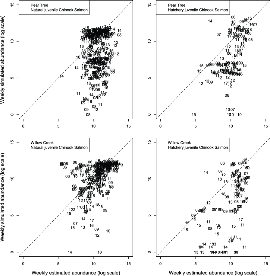
Weekly abundance estimates (log scale) for Trinity River Chinook salmon (Oncorhynchus tshawytscha) that passed Pear Tree and Willow Creek fish traps compared to those simulated by the Stream Salmonid Simulator (S3) model under model 4 that was fit to the weekly abundances at the Willow Creek trap. Data points represent the last two digits of the juvenile out-migration year.
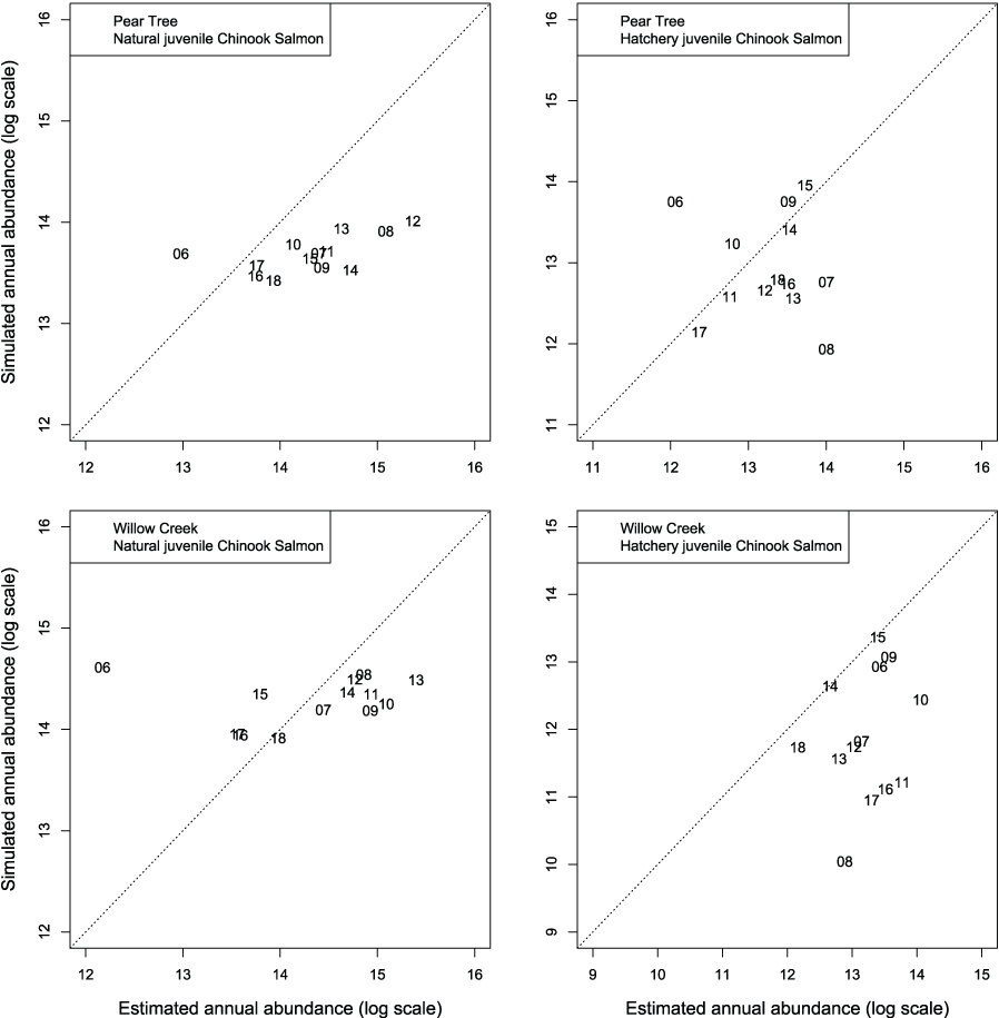
Annual abundance estimates (log scale) for Trinity River fall Chinook salmon (Oncorhynchus tshawytscha) that passed Pear Tree and Willow Creek fish traps compared to those simulated by the Stream Salmonid Simulator (S3) model under model 4 that was fit to the weekly abundances at the Willow Creek trap. Data points represent the last two digits of the juvenile out-migration year.
Appendix 2. Figures for Best Model Fit to Pear Tree Fish Trap Abundances
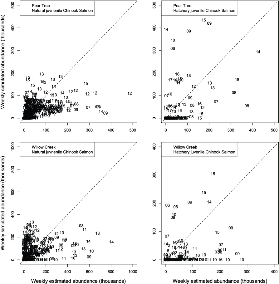
Weekly abundance estimates for Trinity River fall Chinook salmon (Oncorhynchus tshawytscha) that passed Pear Tree and Willow Creek fish traps compared to those simulated by the Stream Salmonid Simulator (S3) model under model 4 that was fit to the weekly abundances at the Pear Tree trap. Data points represent the last two digits of the juvenile out-migration year.
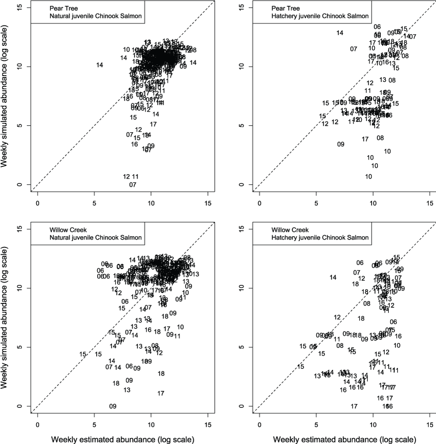
Weekly abundance estimates (log scale) for Trinity River fall Chinook salmon (Oncorhynchus tshawytscha) that passed Pear Tree and Willow Creek fish traps compared to those simulated by the Stream Salmonid Simulator (S3) model under model 4 that was fit to the weekly abundances at the Pear Tree trap. Data points represent the last two digits of the juvenile out-migration year.
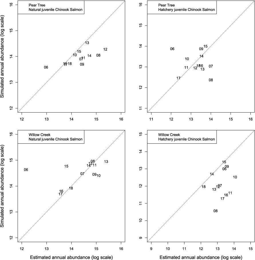
Annual abundance estimates (log scale) for Trinity River fall Chinook salmon (Oncorhynchus tshawytscha) that passed Pear Tree and Willow Creek fish traps compared to those simulated by the Stream Salmonid Simulator (S3) model under model 4 that was fit to the weekly abundances at the Pear Tree trap. Data points represent the last two digits of the juvenile out-migration year.
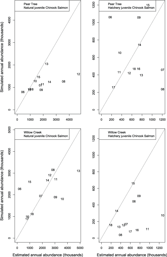
Annual abundance estimates for Trinity River fall Chinook salmon (Oncorhynchus tshawytscha) that passed Pear Tree and Willow Creek fish traps compared to those simulated by the Stream Salmonid Simulator (S3) model under model 4 that was fit to the weekly abundances at the Pear Tree trap. Data points represent the last two digits of the juvenile out-migration year.
Appendix 3. Run-Timing from Best Model Fit to Pear Tree Fish Trap Abundances
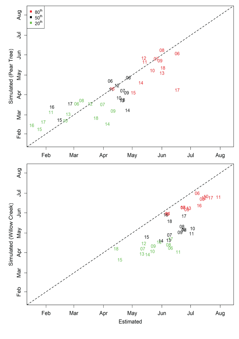
The 20th, 50th, and 80th percentiles in the annual migration dates for Trinity River juvenile Chinook salmon (Oncorhynchus tshawytscha) that passed the Pear Tree and Willow Creek fish traps compared to those that were simulated by the Stream Salmonid Simulator (S3).
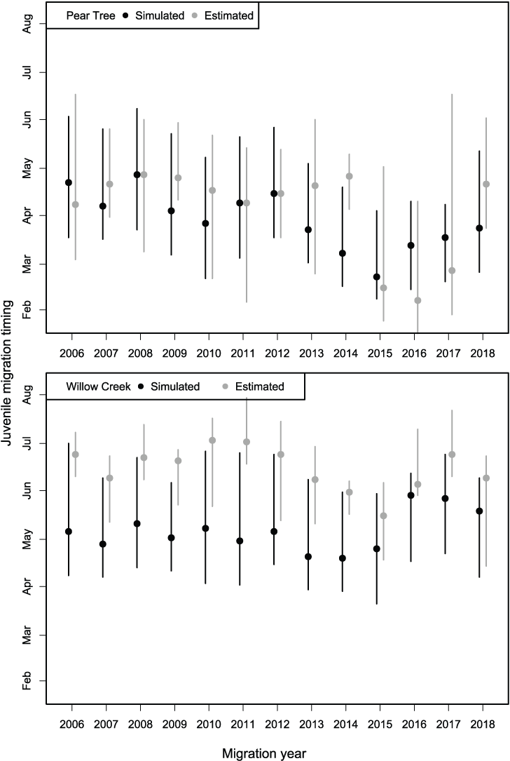
Range from the 20th to 80th percentiles (extent of bars) and the median (data points) for Klamath River Chinook salmon (Oncorhynchus tshawytscha) that passed the Pear Tree and Willow Creek fish traps compared to those simulated by the Stream Salmonid Simulator (S3) model (Model 4) that was fit to the abundance estimates at the Pear Tree fish trap.
Appendix 4. Fish Size Based on Best Model Fit to Pear Tree Fish Trap Abundances
![Graphs showing simulated versus observed fork length of Trinity River Chinook salmon
(Oncorhynchus tshawytscha) that passed the Pear Tree fish trap as estimated from the
model fit to the Pear Tree fish trap. Note that simulated fork-lengths are presented
as a weekly average, whereas the observed fork lengths show the size of individual
fish. Horizontal dashed lines show size cut-offs used to define fry (<50 millimeter
[mm]), parr (51–90 mm), and smolts (>90 mm) in the Stream Salmonid Simulator (S3).](https://pubs.usgs.gov/of/2023/1023/images/ofr20231023_fig04.01.png)
Simulated versus observed fork length of Trinity River Chinook salmon (Oncorhynchus tshawytscha) that passed the Pear Tree fish trap as estimated from the model fit to the Pear Tree fish trap. Note that simulated fork-lengths are presented as a weekly average, whereas the observed fork lengths show the size of individual fish. Horizontal dashed lines show size cut-offs used to define fry (<50 millimeter [mm]), parr (51–90 mm), and smolts (>90 mm) in the Stream Salmonid Simulator (S3).
![Graphs showing simulated versus observed fork length of Trinity River Chinook salmon
(Oncorhynchus tshawytscha) that passed the Willow Creek fish trap as estimated from
the model fit to the Pear Tree fish trap. Note that simulated fork-lengths are presented
as a weekly average, whereas the observed fork lengths show the size of individual
fish. Horizontal dashed lines show size cut-offs used to define fry (<50 millimeter
[mm]), parr (51–90 mm), and smolts (>90 mm) in the Stream Salmonid Simulator (S3).](https://pubs.usgs.gov/of/2023/1023/images/ofr20231023_fig04.02.png)
Simulated versus observed fork length of Trinity River Chinook salmon (Oncorhynchus tshawytscha) that passed the Willow Creek fish trap as estimated from the model fit to the Pear Tree fish trap. Note that simulated fork-lengths are presented as a weekly average, whereas the observed fork lengths show the size of individual fish. Horizontal dashed lines show size cut-offs used to define fry (<50 millimeter [mm]), parr (51–90 mm), and smolts (>90 mm) in the Stream Salmonid Simulator (S3).
Conversion Factors
International System of Units to U.S. customary units
Temperature in degrees Celsius (°C) may be converted to degrees Fahrenheit (°F) as follows:
°F=(1.8×°C)+32
Abbreviations
2D
2-dimensional
>
greater than
<
lesser than
AEAM
Adaptive Environmental Assessment and Management
AIC
Akaike information criterion
CDFW
California Department of Fish and Wildlife
DSS
decision support system
FL
fork length
MHU
meso-habitat units
RBM10
River Basin Model-10
rkm
river kilometer
S3
Stream Salmonid Simulator
TRRP
Trinity River Restoration Project
For information about the research in this report, contact
Director, Western Fisheries Research Center
U.S. Geological Survey
6505 NE 65th Street
Seattle, Washington 98115-5016
https://www.usgs.gov/centers/wfrc
Manuscript approved on March 7, 2023
Publishing support provided by the U.S. Geological Survey
Science Publishing Network, Tacoma Publishing Service Center
Disclaimers
Any use of trade, firm, or product names is for descriptive purposes only and does not imply endorsement by the U.S. Government.
Although this information product, for the most part, is in the public domain, it also may contain copyrighted materials as noted in the text. Permission to reproduce copyrighted items must be secured from the copyright owner.
Suggested Citation
Plumb, J.M., Perry, R.W., Som, N.A., Goodman, D.H., Martin, A.C., Alvarez, J.S., and Hetrick, N.J., 2023, Calibration of the Trinity River Stream Salmonid Simulator (S3) with extension to the Klamath River, California, 2006–17: U.S. Geological Survey Open-File Report 2023–1023, 44 p., https://doi.org/10.3133/ofr20231023.
ISSN: 2331-1258 (online)
Study Area
| Publication type | Report |
|---|---|
| Publication Subtype | USGS Numbered Series |
| Title | Calibration of the Trinity River Stream Salmonid Simulator (S3) with extension to the Klamath River, California, 2006–17 |
| Series title | Open-File Report |
| Series number | 2023-1023 |
| DOI | 10.3133/ofr20231023 |
| Publication Date | June 02, 2023 |
| Year Published | 2023 |
| Language | English |
| Publisher | U.S. Geological Survey |
| Publisher location | Reston, VA |
| Contributing office(s) | Western Fisheries Research Center |
| Description | vi, 44 p. |
| Country | United States |
| State | California |
| Online Only (Y/N) | Y |