

Guidelines for Calibration of Uncrewed Aircraft Systems Imagery
Links
- Document: Report (3.7 MB pdf) , HTML , XML
- Download citation as: RIS | Dublin Core
Executive Summary
This report outlines quality assurance (QA) processes, including radiometric and geometric calibration guidelines, and guidelines for data acquisition and quality control to be followed by U.S. Geological Survey (USGS) researchers for acquiring and processing uncrewed aircraft systems (UAS) data. These QA processes ensure that UAS data can be used for quantitative analysis and are comparable with other standard geospatial data.
Remote sensing data play a critical role in monitoring Earth’s resources. Traditionally, the USGS and Department of the Interior have used well calibrated metric sensors mounted on satellite or aircraft platforms to collect these data. These sensors and platforms are stable, and data have been processed using standard pipelines. These processes ensured that the data are generally consistent with each other and benefitted a diverse group of users. These data are shared among multiple researchers around the world through the internet and other means, using standard formats and metadata.
In the last few years, UAS platforms have democratized the remote sensing data collection further, bringing an unparalleled level of control of time, sensors, and processes to individual researchers. Together with the development of cheaper and lighter sensors and relaxation of prohibitions against UAS operation in the National Airspace System by the Federal Aviation Authority, researchers can collect remote sensing data using UAS platforms. Researchers often customize the sensors on these UAS systems based on their specific requirements and use ad hoc processing steps to generate data.
A challenge is that these data are often produced by a wide array of sensors and processes that render them potentially inconsistent with each other. Therefore, unlike data collected from metric sensors, UAS-based data are designed to benefit only specific user groups. The data thus generated often lack traceability to known standards, making them difficult to use with other geospatial data.
This report provides radiometric and geometric calibration guidelines, as well as guidelines for data acquisition and quality control, that can be followed by USGS researchers in acquiring and processing UAS data. Instead of calibrating sensors, researchers collecting UAS data can focus on calibrating the data. Various radiometric calibration processes are provided, and the two panel empirical line method is highlighted for radiometric calibration.
For geometric calibration, USGS and Department of the Interior researchers are experienced in following standard calibration procedures provided by standard UAS data processing software. However, researchers may be aided in paying attention to the tie points and the accuracy of the ground control points used for geometric calibration and data production. The accuracy of ground control points are related to the requirements of the project. The ground control points and the quality of tie points directly contribute to the geometric accuracy of the data, regardless of the ground sample distance of the imagery.
The guidelines outlined in this report are intended to ensure that the data are in common units and are quantifiable and comparable with other data. These QA and calibration processes can be critical in ensuring that these datasets are used to the maximum extent possible. Including the calibration parameters (and their uncertainties) as part of metadata can allow for easier data discovery and analytical filters.
Introduction
Uncrewed aircraft systems (UAS) have democratized remote sensing data collection for monitoring and mapping. Together with the development of cheaper and lighter sensors, and relaxation of prohibitions against UAS operation in the National Airspace System by the Federal Aviation Authority, researchers can collect remote sensing data using UAS platforms. The various stakeholders and their interests stemming from the guidelines are listed in figure 1.
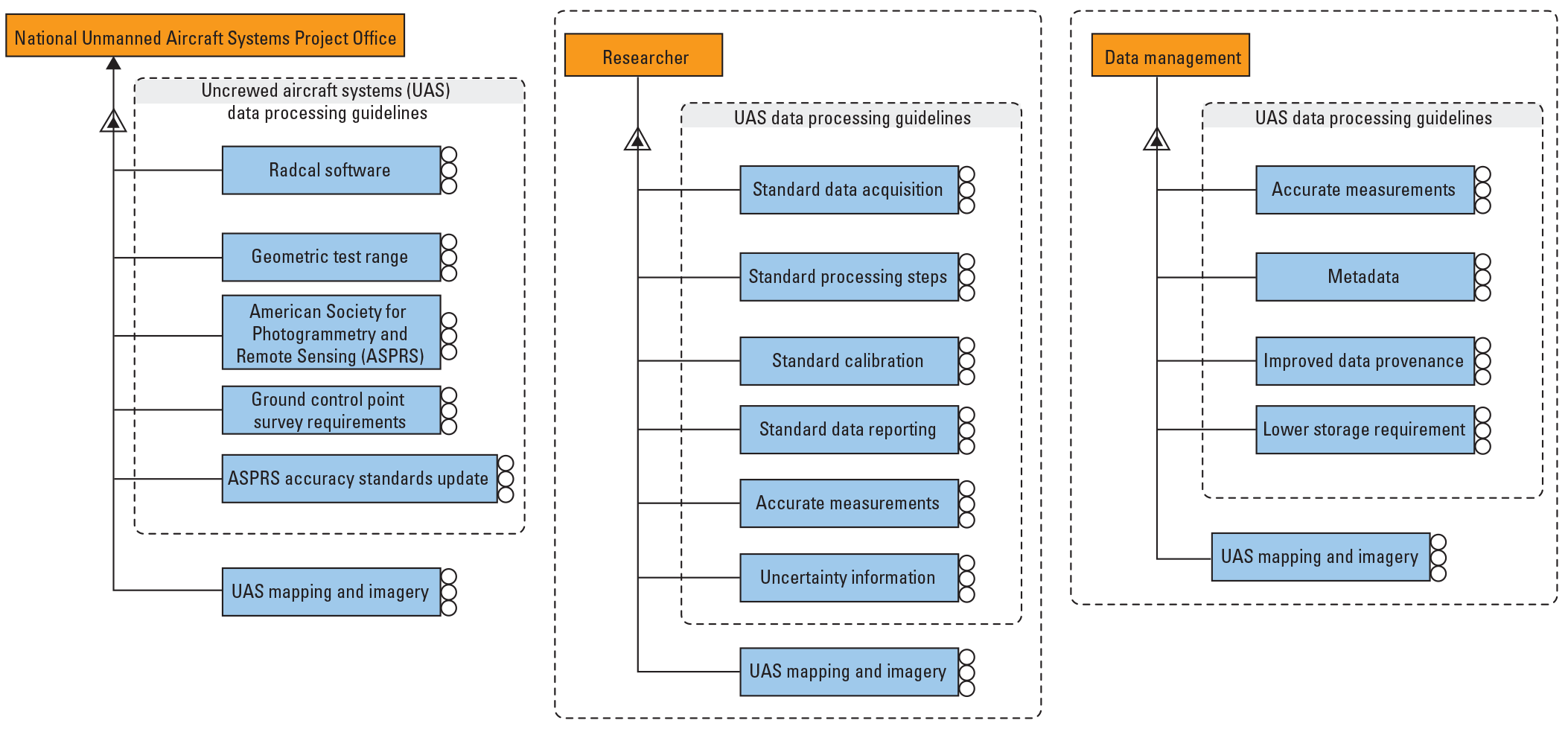
Uncrewed aircraft systems guidelines and their uses to respective stakeholders.
Most of the remote sensing data used by the scientific community (at the U.S. Geological Survey [USGS] and beyond) have been collected using expensive and stable metric sensors, and data have been processed using standard pipelines. These processes ensured that the data are generally consistent with each other and benefitted a diverse group of users. Researchers often customize systems based on their requirements and use ad hoc processing steps to generate data acquired from uncrewed aircraft systems (UAS) platforms.
The value of UAS data to researchers includes the following:
-
• Ability to customize sensors based on research requirements and
-
• Ability to collect data at times when needed by the researcher.
A challenge is that these data are often produced by a wide array of sensors and processes that render the data potentially inconsistent with each other. Therefore, unlike data collected from metric sensors, UAS-based data are designed to benefit limited user groups.
UAS imagery data need to be in the same scale and units as other geospatial data to be used in quantitative research. More specifically, the digital numbers (DNs) measured by the sensors on the UAS platforms need to be relatable to sensor energy radiance or surface reflectance units, which requires the use of radiometric calibration procedures that convert raw DNs measured by the sensor to energy units. Similarly, the metric measurements of size and shape made from UAS imagery and the derived point cloud need to be in common distance units, which requires geometric calibration of the data. Further, the UAS data are being distributed via the USGS EarthExplorer database where they are used by non-USGS and Department of the Interior (DOI) users. The expectation of quality on these products by these users is high. Current data calibration practices followed by USGS and DOI researchers vary in rigor. The use of cheaper, lighter, and mostly commercial off-the-shelf sensors also contributes to varying quality of data. These variations on data quality may be mitigated by using standard procedures for planning, data collection, calibration, processing, verification, and validation. However, even though the UAS-based remote sensing technology has been growing exponentially for more than a decade, a systematic, universal, feasible, and convenient calibration procedure has not been developed to date (Wang and Myint, 2015).
Purpose and Scope
In this report, guidelines for standard radiometric and geometric calibration procedures for UAS data are included. The guidelines are intended to be used by National Unmanned Aircraft Systems Project Office (NUPO) researchers and the USGS Earth Resources Observation and Science (EROS) Center for data management. The included quality assurance (QA) and calibration procedures can be critical in ensuring that UAS datasets are used to the maximum extent possible. Including (radiometric and geometric) calibration parameters (and their uncertainties) as part of the metadata can also allow for easier data discovery and analytical filters. These documentations can make it easier to decide whether the data can or cannot be used for a certain application. To help the USGS achieve this goal within the UAS community and provide the USGS and EROS with the ability to acquire and distribute such data, the following are required:
Remote Sensing
Remote sensing has played a vital role in monitoring and quantifying the changes on the Earth’s surface because of natural or anthropogenic effects at regional, continental, and global scales. However, the limitations of some platforms for remote sensing, including satellite platforms, are high cost, lack of spatial resolution for the identification of ground traits, cloudy scenes preventing the view of ground traits, and long revisit times (Han-Ya and others, 2010; Gevaert and others, 2015). Generally, satellite acquisition of the Earth’s surface is limited by its fixed orbital pattern, which is further curtailed by cloud cover and consumer demand for resolutions higher than those offered by orbital satellites. Piloted airborne systems capture high-resolution imagery in a timely manner but are often cost prohibitive (Rango and others, 2009). UAS occupy a previously unfilled niche through their capacity to generate the high-resolution imagery on a flexible temporal scale (Dunford and others, 2009). UAS offer the scientific community and other users an unprecedented level of accessibility and flexibility of data generation to address individual research interests and issues (Kelcey and Lucieer, 2012). Therefore, UAS has become a viable alternative to conventional satellite and airborne platforms for acquiring high-resolution imagery (Everaerts, 2008).
Uncrewed Aircraft Systems Remote Sensing
In recent years, UAS applications have become an ever-expanding area in remote sensing driven by scientific and commercial success (Pajares, 2015). This expansion has been attributed to the low cost, versatility, and continued technological development associated with UAS, which has increased their performance and made them useful for an ever-increasing range of applications, including (a) agriculture and forestry (monitoring crop health, precision agriculture, environmental monitoring), (b) firefighting (forest fires, emergency rescue), and (c) Earth observation and remote sensing (aerial photography, mapping, and surveying). Technological development in electronics and plastics has resulted in producing lightweight navigation systems, controllers (Joseph and others, 2016), and lightweight plastic chassis with comparable mechanical strength of the previous metal chassis (Zhu and others, 2004). These weight reducing strategies have resulted in increased flight time capacity (Lee and others, 2020). Given the relative economy of UAS and their continued technological improvements, the use of UAS will likely increase to include a wider range of applications in the next 5 years; therefore, establishing a standard method of image calibration and increased data quality would be beneficial.
The advantages of using UAS for remote sensing are many:
-
• High spatial, spectral, and temporal resolution at a low cost compared to satellite and aerial platforms.
-
• Minimum atmospheric effect on the radiance recorded by the UAS sensor. This effect generally is ignored because the UAS sensor flies close to the ground surface (about 200 meters above); therefore, it passes through a small column of atmosphere, limiting atmospheric effects (Iqbal and others, 2018).
-
• Increased versatility. UAS can be deployed on a cloudy day if the cloud cover resides above the UAS flight path, allowing for image acquisition when satellite imaging would be hindered by cloud cover.
Radiometric Calibration
All remote sensors record data in arbitrary units, referred to as “DNs.” Without a calibration to physical energy properties of the site, such as radiance, reflectance, or temperature, the DNs are without meaning and of no use for further scientific analysis; therefore, consistent, accurate, and reproducible calibrations are required for all UAS data acquisition intended for scientific studies, and calibration is a prerequisite for any optical sensor collecting data for scientific study.
UAS-derived imagery ideally would be radiometrically calibrated to maintain spectral consistency during the field campaign (Smith and Milton, 1999). Spectral consistency allows users to compare the data acquired on different days and at different times within a day. UAS-acquired data become more versatile and useful to the scientific community when they are radiometrically calibrated to the target’s radiometric properties.
Theoretical Perspective
Calibration of remote sensing data is necessary for the data to be useful to the scientific community (Helder and others, 2018). Calibration can be done using two methods: sensor calibration and image calibration. Sensor calibration is used to calibrate well calibrated scientific grade mission sensors such as the Operational Land Imager (Landsat), Thermal Infrared Sensor (Landsat), Multispectral Instrument (Sentinel 2), and Moderate Resolution Imaging Spectroradiometer. The sensors aboard each spacecraft are rigorously characterized before and after launch to maintain their data quality. Teams of scientists and technicians have worked to minimize the uncertainty of the associated data products. Calibration activities continue throughout the life of the sensor, which can be more than 20 years, as was the case for Landsat 5, which provided copious high-quality images of the Earth for the global scientific and commercial communities.
Sensors in Landsat missions are calibrated because each of these programs selected a single sensor type, which could be procured from a single manufacturer, and the deployment environment (space) was well controlled. Further, bias could be easily acquired from shutter for reflective bands and deep space and black body for thermal bands. A coordinated team of scientists and technicians monitor, recalibrate, and publish the data acquired, ensuring a standard format of archived data that can be shared with the global community.
Sensor-based calibration is not feasible for a UAS-based system because many different sensors are available from many different manufacturers; have variable platforms; and are deployed by numerous individuals in the private, academic, commercial, and government sectors. Therefore, standardization of UAS sensors would be a monumental task. However, there is a simple alternative: calibrate the UAS image instead of its sensor. A single process change, the addition of standardized target panels at the acquisition site, is required to implement image-based calibration. The standardized target panels would need to be well characterized at various spectral energies with correction factors assigned to each spectral energy of interest. The panel correction factors are essential for the conversion of the DN to a physical site property such as reflectance, which is the “common language” across many remote sensing customers. Correction factors are easily acquired from either the manufacturer of the panel or through characterization of the panel by the data collection team. Image-based calibration can transcend the difficulties associated with the variety of platforms, sensors, manufacturers, and image contributors currently present in the UAS realm because they are sensor independent.
Image-based calibration for UAS images would be superior for at least three reasons:
-
• Variable users would use the same calibration approach, providing a universal standard all product users could easily adopt. Currently, each UAS manufacturer has a different calibration approach for their sensor, which is not universal or standard; therefore, comparing UAS products from different manufacturers, or even the same manufacturer, is problematic. However, an image-based calibration approach allows for direct comparisons of different UAS products through a common characteristic of interest like reflectance.
-
• Many different instruments can be used because the calibration method is sensor independent while meeting the end user goals. Many users want data that can be easily analyzed, published, peer reviewed, and replicated but are not necessarily interested in how those goals are completed. Image-based calibration of UAS products would allow these data to be provided in a simple, economically palatable process that is sensor independent.
-
• Most users prefer to know the reflectance of their target rather than the associated radiance because reflectance is illumination intensity independent whereas radiance varies with the illumination source intensity.
Image-based calibration is the most fundamental method to correlating the DN recorded by the sensor to reflectance. It requires ground measurements of reflectance at several known targets to produce reliable, repeatable results (Smith and Milton, 1999). One common way of determining the empirical relation between the sensor DN and corresponding reflectance is the empirical line method (ELM).
Empirical Line Method
ELM is the most widely used calibration technique for UAS images to date because it is simple, effective, and easily implemented in the field (Smith and Milton, 1999). ELM assumes that the image consists of one or more calibration targets of different reflectance covering a wide range of reflectance values for the wavelengths recorded by the sensor. Although this method is simple, effective, and straightforward, nuances exist that warrant careful management to avoid acquiring erroneous results; for example, choosing reflectance targets that encompass the reflectance range of the surfaces within the scene is important. Additionally, careful and thorough characterization of the spectral properties of the calibration targets is equally important for accurate image calibration (Smith and Milton, 1999). Further, this method has been implemented using one calibration target by using the bias reported by the manufacturer or taking an image with the shutter closed. Clearly, this is not a true bias because imaging a zero-reflectance panel would not result in the same value as the laboratory-acquired bias nor the closed shutter bias; therefore, the calibration curve would not be as accurate as taking two or more calibration target images. It is worth noting that most researchers use two (Ben-Dor and others, 1994; Dwyer and others, 1995; Laliberte and others, 2011), four (Farrand and others, 1994; Price and others, 1995), or more calibration targets to improve calibration accuracy.
One-Point Method
Single calibration target implementation of ELM assumes that a surface with zero reflectance will produce zero radiance at the sensor. It does not account for atmospheric light scattering recorded by the sensor. The dark point is the first calibration point, and the second point on the calibration curve is the single target of known reflectance, taken as the bright target in the image. The calibration target is well characterized spectrally across all wavelengths to be measured. With the dark point and bright point (a well characterized calibration target), a calibration curve is constructed for the image. The calibration coefficient (gain of the straight line; that is, slope) is used to convert the DNs of the image to a physical unit, usually reflectance or radiance. Freemantle and others (1992) and McArdle and others (1992) used the single point calibration method for their images and reported 20-percent and 15-percent error, respectively.
Two-Point Method
An improvement over the one-point method is the two-point method. By using two well characterized calibration panels of known reflectance, one dark and one bright, preferably encompassing the reflectance range within the image, a calibration curve more closely aligning with the actual reflectance of the image can be acquired. The camera or spectrometer records the DN for both the panels. Using the same technique mentioned in the one-point method, a calibration curve is created by drawing a line between the two calibration target points as shown in figure 2. Calibration coefficients (gain and bias) are acquired by establishing a relation between the measured DN and reflectance of the calibration panel. The calibration coefficients are used to assign reflectance to all other DNs. Several researchers (Kruse and others, 1990; Ben-Dor and others, 1994; Dwyer and others, 1995; Ferrier and Wadge, 1996) have used this two-point method. They have generated reasonable calibrations; however, studies (Fawcett and Anderson, 2019; Mamaghani and Salvaggio, 2019) have documented the benefits of ELM-based calibration quantitatively.
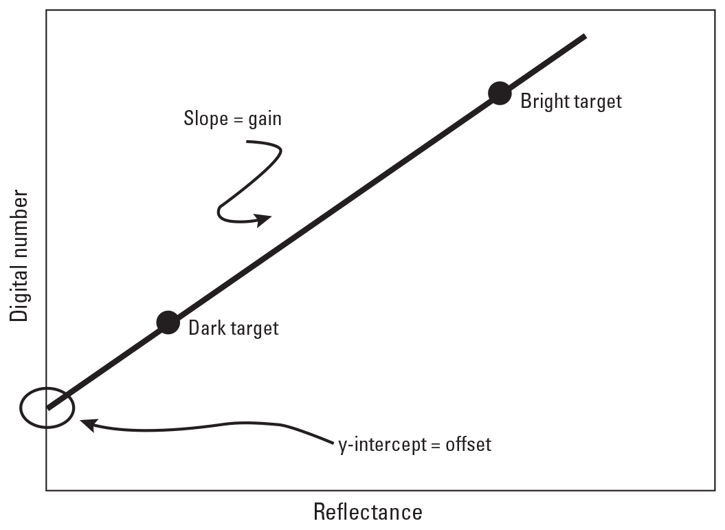
Gain and offset derived from a single channel via the empirical line method (Farrand and others, 1994).
A potential drawback to the two-point ELM is it assumes that the sensor response is linear in nature. However, some work has been done using more than two calibration targets to accurately determine the relation between radiance recorded by a sensor and its corresponding reflectance, thus removing the linear relation assumption (Iqbal and others, 2018). Farrand and others (1994) and Price and others (1995) illustrated the value of additional calibration targets by demonstrating the improvement in calibration results using four calibration targets. Nonlinearity seems to be consolidated in the extreme reflectance ranges, either very dark or very bright. The assumption of linearity in the middle range seems to be reasonable.
Although ELM is a common calibration method, it has some limitations based on some fundamental assumptions. The first assumption is the illumination of the target site is constant throughout image acquisition; however, illumination varies throughout the flight because the solar angle changes during the flight. The second assumption is all surfaces measured are Lambertian in nature, which is not true. Earth’s surfaces demonstrate bidirectional properties, which means reflectance varies with solar and viewing angle changes.
Predetermination of Sensor Bias
The predetermination of the sensor bias method is similar to the one-point ELM explained in the “One-Point Method” section. The objective is to acquire the calibration coefficients via the calibration curve obtained through the bias and one bright calibration target point. Two approaches can be used to determine the sensor bias. The first is to use the calibration bias published by the sensor (camera) manufacturer. The manufacturer obtains the bias by measuring the dark current and uses the energy recorded by the sensor at zero input (zero radiance) during laboratory characterization of the camera. The second approach takes a dark current measurement before the field campaign by recording the sensor measurement when the camera lens is covered (that is, the shutter is closed), which is a zero-radiance measurement.
Calibration Panel
The calibration panel is the most important part of an image-based calibration approach because it is the basis for the acquisition of calibration coefficients used to adjust all the UAS image pixels to a standard calibration. Therefore, the panel material and size are of extreme importance and should be considered carefully before a UAS campaign is started. The type of panel material and its size are briefly discussed in the following sections.
Panel Material
In the early days of ELM, researchers used a natural calibration target. Freemantle and others (1992) used a road as a calibration target, McArdle and others (1992) used the top of a gray water tank, and Price and others (1995) used gravel rooftops and a patch of snow for calibrating their image using ELM. These researchers reported an error of 10–20 percent predicted reflectance using the derived calibration coefficients. The material used for a calibration target substantially affects calibration accuracy; therefore, researchers implementing ELM recently have been using more accurate calibration targets to enhance their calibration accuracy. Most calibration panels that were used are pressed and painted barium sulfate powder panels and pressed polytetrafluoroethylene powder panels (Jackson and others, 1992). There panels are expensive as they are robust and technically difficult to manufacture. Wang and Myint (2015) studied 10 different materials that are cost-efficient and easy to transport, and they reported that Masonite hardboard had optimal radiometric properties that met their calibration criteria for their UAS campaign. Among different calibration panels, Spectralon targets are used for field applications that require long exposure to harsh environments (Pro-Lite Technology, Ltd., 2022) due to their robustness. These targets demonstrate near Lambertian characteristics, which help to maintain constant contrast over a wide range of viewing and solar geometry. Because of these properties, these targets have been widely used by different calibration groups in ground site validation campaigns for well calibrated sensors such as the Operational Land Imager, Thermal Infrared Sensor, and Multispectral Instrument. In addition, compared with painted targets, Spectralon is durable, washable, and waterproof (Pro-Lite Technology, Ltd., 2022), which are useful characteristics for UAS calibration. UAS teams can use calibration panels consisting of material that meets their calibration criteria. A “self-made” calibration panel can be used if it is well characterized; that is, its reflectance at variable electromagnetic wavelengths is reported. Reflectance measured at variable viewing and solar angles is measured and reported, and its property changes over exposure time (degradation) are reported/measured.
Panel Size
Calibration quality is affected by the number and quality of pixels imaged from the calibration panel; therefore, the calibration panel size warrants consideration during UAS calibration using ELM. The panel ideally would be large enough to include adequate “pure” pixels in the UAS image. Pure pixels are the pixels that have minimum adjacency effects. Generally, the pixels at the side of a calibration target are more susceptible to this effect because they contain additional signal scatters off the objects residing nearby. Maximizing “pure” pixels so that intrinsic variability of the pixels can be reduced through averaging is the method used to obtain the true reflectance of the calibration panel. Smith and Milton (1999) indicated that the side of the calibration target should be at least several times larger than the sensor ground field of view. Wang and Myint (2015) quantified the relation between panel and pixel size and indicated that the side of a calibration target should be at least 10 times larger than the maximum possible pixel size to achieve enough “pure” pixels for UAS calibration.
Sensor Correction
Sensor correction is done for dark current correction and vignetting correction.
Dark Current Correction
Dark current is a residual current that flows through photosensitive devices when there is no input radiation (Sarkar and others, 2013). Dark current is measured by capturing several images with the lid of the camera closed. The dark current of each detector is calculated by taking an average of those captured images. The estimated dark current value of each detector/pixel is subtracted from every image before any further processing.
Vignetting Correction
Vignetting effect in the sensor is due to radial falloff of illumination at the edge of the image. This effect is position dependent and arises as a sensor component (aperture) blocks the light energy from the detector at a wide angle (Yu, 2004; Goldman, 2010) as shown in figure 3. The vignetting effect degrades the image quality of the sensor as the radial shadowing effect increases towards the image periphery.
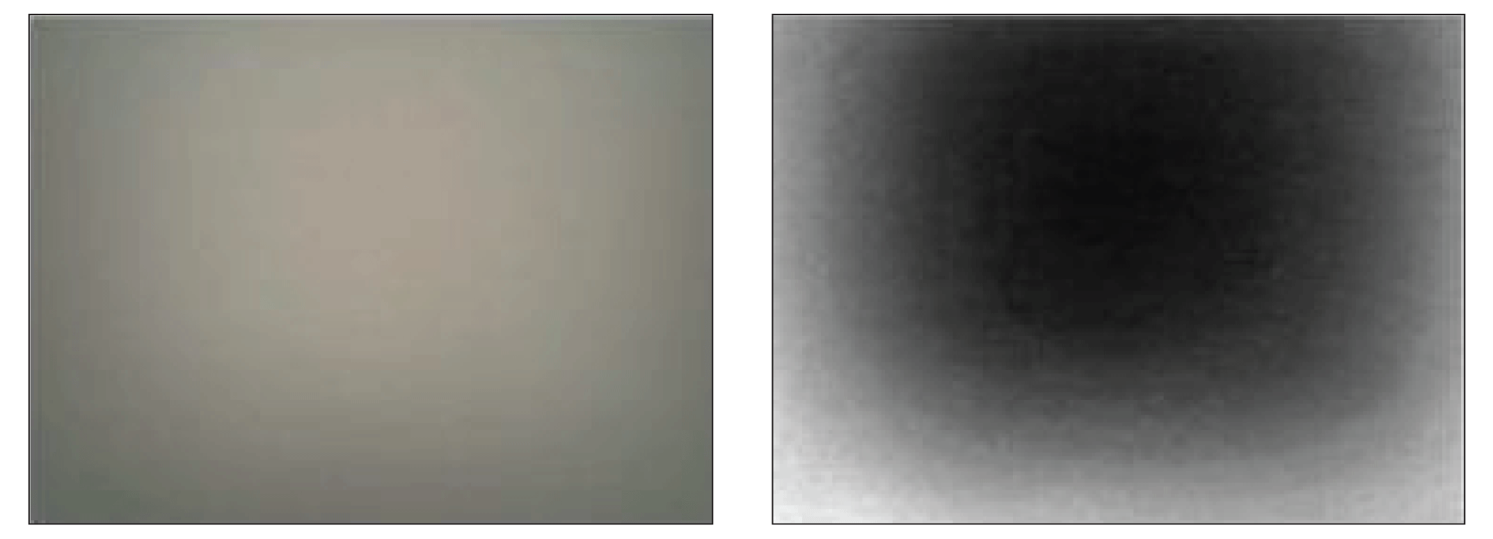
The vignetting effect (left) and its correction factor (right; Yu, 2004).
Vignetting correction is completed by modeling the radial illumination falloff. For this modeling, a flat field surface is used as a reference. Flat field surfaces are the surfaces that demonstrate uniform, spectrally homogeneous Lambertian properties (Mansouri and others, 2005). A flat field surface is imaged multiple times, which demonstrates the radial illumination falloff from a homogeneous condition at the edge of the image. The brightest or center pixel value of these images is considered the true flat field measurement and is used as a reference to calculate the correction factor for the rest of the pixels. Such a derived per-pixel correction factor, as shown in figure 3, is used to restore the true flat file value in every pixel of an image (Yu, 2004; Mansouri and others, 2005). As the illumination decreases towards the periphery of an image, the correction factor increases towards the periphery to compensate for the fading illumination within the image.
Bidirectional Reflection Distribution Function
The bidirectional reflection distribution function (BRDF) describes the interaction of light with a given point on the surface by relating the incoming and outgoing radiance at that point. Formally, BRDF quantifies the radiance scattered in all directions from the surface illuminated by the source from any direction. Mathematically, BRDF is given by the following equation:
wherefr
is the BRDF of the surface;
is the incident zenith angle, in units of degree;
is the incident azimuth angle, in units of degree;
is the reflected zenith angle, in units of degree;
is the reflected azimuth angle, in units of degree;
is the wavelength, in units of nanometer;
dLr
is the spectral radiance leaving the surface, in units of Watt meter−2 steradian−1 nanometer−1; and
dEi
is the irradiance illuminating the surface, in units of Watt meter−2 steradian−1 nanometer−1.
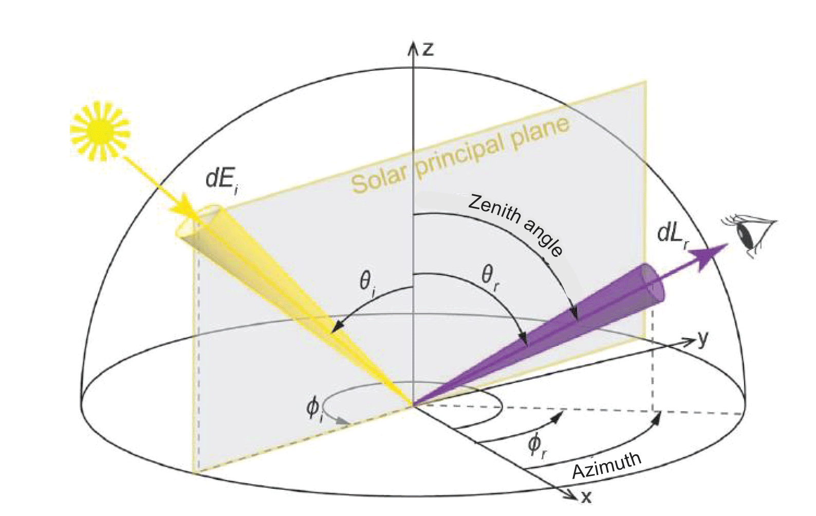
Concept of incident and reflected angles in spherical coordinate system (adapted from Doctor and others [2015]). [x, y, and z represent the three directions in three dimensional space]
Most of the Earth’s surface is non-Lambertian in nature; thus, its reflectance varies with the viewing and solar geometry. This phenomenon is called the BRDF effect. The BRDF effect is inevitable for all optical satellite sensors, and its magnitude depends on the magnitude of viewing and solar geometry; that is, optical systems having a narrow field of view have smaller BRDF effects (Roy and others, 2016). However, a change in the illumination angle also contributes to the BRDF effect so, despite a narrow field of view, BRDF effect should be corrected to improve the data quality and, hence, radiometric calibration. Calibration teams of different well calibrated sensors, such as those present on Landsat, Sentinel 2, Moderate Resolution Imaging Spectroradiometer, and so on, have used different types of BRDF models to improve their calibration accuracy (Wu and others, 2008; Helder and others, 2013; Farhad and others, 2020). In UAS imagery, it is important to address the BRDF effects to compare the reflectance observed for a surface at different viewing and illumination geometries.
Radiometric Calibration Steps
This section briefly describes the steps to follow during the field campaign. It highlights the importance of camera setting, dark current measurement, and panel measurement to improve the data quality.
Data Acquisition During Field Campaign
A rigorous literature search was completed for UAS radiometric and geometric calibration methods. Some of the theoretical findings have been mentioned in previous sections. Based on the findings from the literature search and discussion among the team members, the following steps are outlined to improve radiometric and geometric calibration of UAS data acquired during a field campaign.
Before the site is measured, choose a location to place the calibration panels such that the UAS captures an image of them at the beginning and end of each flight. The more frequently these panels are imaged, the greater the enhancement of the image quality. Optimally, calibration panels would be captured every 10 minutes during flight; however, because most UAS have a fuel capacity for about 15 minutes of flight, panels may be minimally imaged at the beginning and end of each flight. Generally, the panels are placed at the same location as UAS takeoff and landing.
Checking Camera Settings
Manual setting of the camera allows gain and shutter speed to be kept constant during the flight. The appropriate gain and shutter speed of the camera should be set. The dynamic range of the camera should be maximized for the intended target; that is, maximum vegetation reflectance in the near-infrared band is around 0.5; therefore, the camera should be set in such a way that it will saturate around 0.6, which will increase the radiometric resolution of the camera. These steps will provide better resolution than when saturation is set at 1 reflectance unit (100-percent reflective) when imaging vegetation that has a maximum reflectance value of 0.5.
The automatic setting can be used but the camera should record the setting used while capturing the image. Each image will have a different set of settings if “automatic” is selected; therefore, for optimal radiometry, the camera should be calibrated in each setting combination. Manually selecting the camera settings ensures the settings remain constant and decreases the amount of sensor calibration necessary for accurate radiometric imaging; however, the images themselves may appear blurred.
Data Processing
This section briefly describes the steps that are needed to process raw digital number to physical quantities such as radiance and reflectance.
Bias Correction
Bias for the camera is estimated by averaging the images collected with the aperture closed. Before any further processing, subtract the bias from UAS imagery. Bias estimation for the camera also is provided by its manufacturer; however, as sensor responsivity changes, bias calculated during the field campaign will be a more accurate estimation of dark current than bias provided by the manufacturer.
Vignetting Correction
Vignetting refers to radial fall off of pixel intensity from the center towards the edge of an image. A correction factor should be applied to remove this effect. Generally, camera manufacturer provides this correction factor. For example, MicaSense (2022) provides a radial vignette model to correct the radial fall off the illumination at the edge of the image. To apply the model, cx, cy, and six polynomial coefficients are provided in the metadata file. This information can be used to calculate a per-pixel correction factor by applying the following equation (MicaSense, 2022):
wherer
is the distance of the pixel (x, y) from the vignette center, in pixels;
(x, y)
is the coordinate of the pixel being corrected;
cx, cy
are the center coordinate of vignetting center pixel;
ki
i = 0,1,2,3,4, and 5 is a polynomial coefficients that generates correction factor for any pixel;
K
is the correction factor by which the raw pixel value should be divided to correct for the vignette;
I(x, y)
is the original intensity of the pixel at x, y; and
Icorrected(x, y)
is the corrected intensity of the pixel at x, y.
Camera Corrections
All the passive remote sensing devices go through some level of laboratory calibration to determine radiometric calibration coefficients. Radiometric calibration coefficients helps to convert raw digital recorded by sensor to physical quantities such as radiance and reflectance. For example, sensor manufacturers often provide a radiometric calibration model that converts the raw pixel values of an image into absolute spectral radiance values. The model compensates for sensor black level, the sensitivity of the sensor, sensor gain and exposure settings, and lens vignette effects. For example, MicaSense provides the formula for computing the spectral radiance from the pixel value as follows (MicaSense, 2022):
whereL
is the spectral radiance, in Watt per square meter per steradian per nanometer (W/m2/sr/nm);
V(x, y)
is the vignette polynomial function for pixel location (x, y);
x, y
are the pixel column and row number, respectively;
a1, a2, a3
are the radiometric calibration coefficients;
p
is the normalized raw pixel value (the normalized pixel value is calculated by dividing the raw DN for the pixel by 2N);
N
is the number of bits in the image (MicaSense cameras save images either in a 12-bit or 16-bit format);
pBL
is the normalized black level value;
g
is the sensor gain setting; and
te
is the image exposure time.
Applying the Empirical Line Method
After completing all the camera corrections, the ELM can be applied using the bright and dark calibration panel measurements, as shown in figure 5 and equation 4:
whereρ(x, y)
is the pixel reflectance,
ρBright
is the bright reflectance panel,
ρDark
is the dark reflectance panel,
Lʹ(x, y)
is the input pixel value,
LʹBright
is the average pixel value of the bright pixel, and
LʹDark
is the average pixel value of the dark pixel.
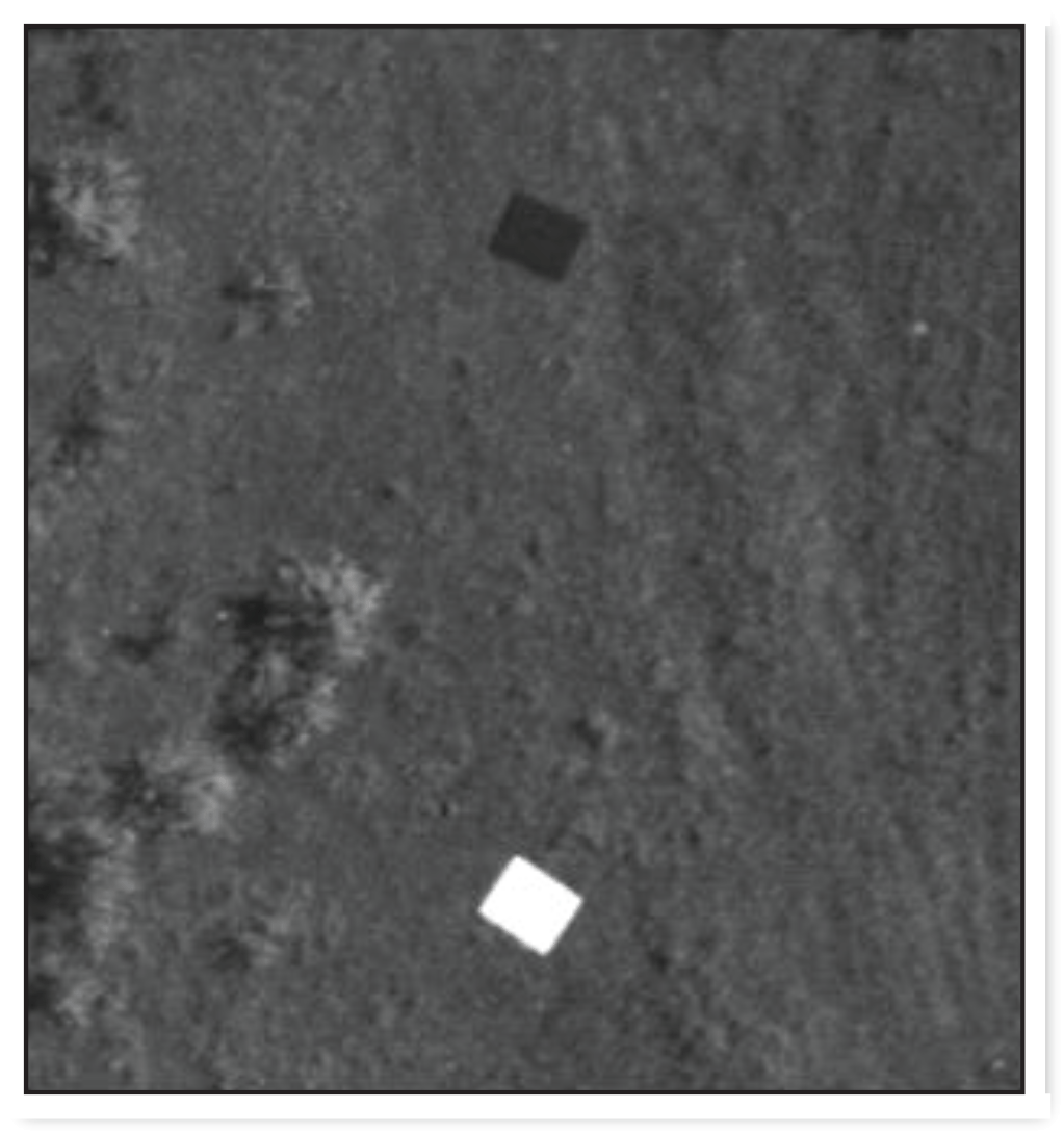
Bright and dark panels during an uncrewed aircraft systems field campaign.
Interpolation Across Images
If there is only one set of calibration panels, follow steps mentioned in the “Applying the Empirical Line Method” section; if there are two sets of calibration panels, then calibration information can be interpolated across the first and second sets of calibration panel measurements to improve calibration accuracy of UAS images as follows:
wherei
is the parameters after (i−1) minutes of the first acquisition of the calibration panels,
i
1 is the acquisition time for the calibration panels at the beginning of the flight,
i
N is the acquisition time for the calibration panels at the end of the flight,
m1
is the slope of the line at the beginning of the flight,
mN
is the slope of the line at the end of the flight, and
mi
is the slope of the line after (i−1) minutes of the first acquisition of the calibration panels.
Field Data
Careful data collection is as important as communicating the information to the global community. Therefore, this section includes a minimal list of items to be included in a final report. This section is intended to provide guidance regarding the information necessary to make the acquired data useful and reproducible for as many users as possible.
Equipment List
An equipment list is not only important for the users of the data, but it also serves as an important planning tool for beginning a field campaign. Once the purpose of the campaign has been determined and the physical aspects to be measured have been determined, then a list of necessary equipment can be developed. The final field report should include all the equipment used, the manufacturer, model number, specifications, and settings; for example, determine how to refer to the camera, an analytical spectroradiometer, a thermal sensor, and so on and remain consistent throughout the data acquisition, data reporting, and final report. If a commercial reflectance panel was used, make sure the manufacturer and correction factors are reported. Including this information in a README file where the raw data reside will facilitate communication across groups and to various users if the intent of the campaign is to produce information that can be used outside the acquisition team.
Reflectance Panel Specifications
Even when a commercial panel is used, field characterization of that panel can be acquired quickly and easily by placing the panel as flat as possible at the scene (using a bubble level). Taking an image of the panel at 0-, 90-, 180-, and 270-degree (°) rotations will provide a quick image analysis of the reflectance pattern for that panel. Additionally, by taking images of the panel at a 0° rotation and rotating the sensor by 0, 90, 180, and 270°, any image anomalies residing within the sensor can be easily identified.
Alternatively, “self-made” panels can be used if they are fully characterized. The material that was used and why should be described. As many characterization properties as possible regarding the material and the panels should be provided, including how the panels were prepared, painted, and dyed; if the panels were made with a three-dimensional (3D) printer, the resin/dye formula and how reflectance was determined for the panel should be included.
The panel size, how many “pure” pixels were acquired, and how that was determined should be included in addition to how a stable flight altitude was obtained and what that altitude was. The anticipated size of the pixel and how that size was maintained throughout the acquisition process should be reported.
This information is of interest to anyone desiring to use the data acquired for their own analysis; therefore, including this information in a README file where the raw data exist would be a good practice.
Bias Method
How the bias was acquired substantially affects the accuracy of the reflectance calibration; therefore, a detailed description of which bias method was used should be included in the final report. The description also should be included with the data files. Consider including this information in a README file where the raw data reside.
Image Acquisition
A planned pattern for image acquisition of the ground site should be determined before the campaign and walked/surveyed with the UAS before image acquisition to ensure the site meets all the anticipated criteria. Including this pattern in the final report would be of interest to the end users. Once the image acquisition pattern has been determined and surveyed, acquisition of the images can begin. The precise time, altitude, and location of each image taken (including the calibrated panel images) are useful for determining the BDRF because the BDRF changes continuously. A description of the flights, altitude, time in flight, refueling times, weather, and cloud cover would be useful as well. Including these descriptions in a README file in the same directory as the raw data facilitates communication with end users.
Reflectance Calibration Curve
The most important tool used on the raw data is the calibration curve. As described previously, the ELM is applied after all the image corrections for the camera, bias, and vignetting effects. The ELM produces a final product in a “universal” language: reflectance. How the ELM was applied will determine its expected accuracy and reliability; therefore, a thorough explanation regarding how many calibration panels were used, when and where they were imaged, and which formulas were used to acquire the reflectance values is the most important information that can be shared regarding the field acquisition.
Geometric Data Quality
UAS data (imagery) generally have high planimetric (x−y) accuracy as compared to data obtained from conventional aerial photogrammetry, even though most of the UAS data are collected using off-the-shelf and nonmetric cameras. This high planimetric accuracy can be attributed to the lower flying height of the UAS platforms during data acquisition. The vertical accuracy of the data (point cloud) is often dependent on the texture of the surface being imaged. The quality of any geospatial data can be maximized by following the principles of QA and quality control (QC). Toth and Jóźków (2016) describe QA as a set of all activities that need to be completed to ensure that the quality of data meets the required standards and QC as the set of activities that verify the data quality meets the requirements of the project. By adapting this definition to UAS-based data collection, the most important set of QA practices includes the following:
The previously mentioned tasks are all interrelated. Calibration is usually completed in the field using the process of “self-calibration”; therefore, the data acquisition process (for example, flying height, flight patterns, overlap, and so on) and the placement of GCPs become an integral part of calibration. The guidelines reflect this interdependence. The USGS and DOI researchers and users of UAS data generally use software-based self-calibration procedures for calibrating data for the following reasons:-
• Researchers do not have the means to ensure the most optimal flight configuration for self-calibration.
-
• Researchers do not have the means to assess the quality of calibration.
-
• Researchers do not have resources to collect sufficient ground check points because of the following:
Data Acquisition
Data acquisition best practices are important for ensuring the overall accuracy of data. Current practices have yielded good results, particularly for ensuring the accuracy of orthophotographs. However, for 3D accuracy, and because of the prevalence of self-calibration processes for cameras, the data acquisition procedures need to be documented and tested.
Ground Control Points
The spatial positioning and accuracy of the GCPs used for data acquisition play an important role in the overall accuracy of UAS data. GCPs can be obtained using survey grade global positioning system/global navigation satellite system (GNSS) receivers or using a combination of GNSS methods and total station based conventional surveying techniques. For the best accuracy (subcentimeter), total station based methods can be used along with published high accuracy benchmarks. Such benchmarks are often documented and maintained by survey organizations such as the National Geodetic Survey or State and national departments of transportation. Another method is to create project benchmarks by occupying these locations with survey grade GNSS receivers for several hours on multiple occasions.
It is important to note that the accuracy of these GCPs need to be at least three times the required accuracy of UAS imagery. The accuracy of the UAS data, therefore, has no direct relation with the ground sample distance (GSD) of the pixels of the imagery. Therefore, a dataset with a 1-centimeter (cm) GSD may well have an accuracy of less than 6 cm (at 1 sigma) if the GCPs have an accuracy of 2 cm or less at 1 sigma. Care is needed by the researcher or user of the UAS imagery to not assign higher accuracy to the imagery just because the GSD is lower. On the other hand, a lower GSD allows the user to identify documented and other kinds of targets on the ground, which in turn, helps achieve higher accuracy for the data.
The USGS EROS Center has been unable to test using a variable number of GCPs because of limitations imposed by the DOI’s grounding of UAS flights for nonemergency missions under Secretarial Order 3379 issued on January 29, 2020 (https://www.doi.gov/sites/doi.gov/files/elips/documents/signed-so-3379-uas-1.29.2020-508.pdf).
Data Acquisition Flight Patterns
It is recommended that UAS data be acquired using two flight elevations, flown in orthogonal orientation (fig. 6); for example, let us say east-west flights are normal data collection flights. The north-south flights are flown at a 50 percent higher elevation such that the ratio of the number of control points to the number of photographs is 4 times higher (for the north-south flights). The north-south flights would not be used to generate final data but will be used only for the alignment and calibration of camera parameters of the east-west flights (that is, for the exterior and interior orientation of east-west flights).
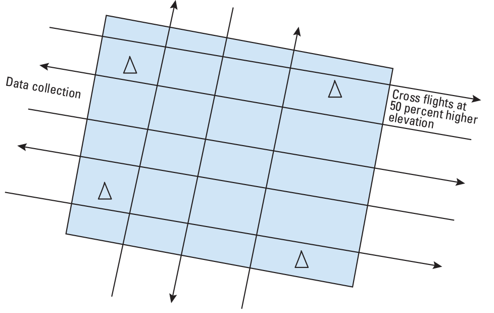
Suggested flight lines for data acquisition to maximize the ratio of control points to the number of photograph frames. The “triangle” symbols are the locations of ground control points.
In a limited set of experiments completed in Granby, Colorado (fig. 7), data were acquired in the suggested flight pattern, along with 11 signalized GCPs. The GCPs were acquired with an average accuracy of 1 cm in the x-y directions (1 sigma) and 2 cm in the z direction (1 sigma). From the discussion in the previous section, “Ground Control Points,” the image data should not be expected to be more accurate than 2 cm in the x-y directions and 5.1 cm in elevation.
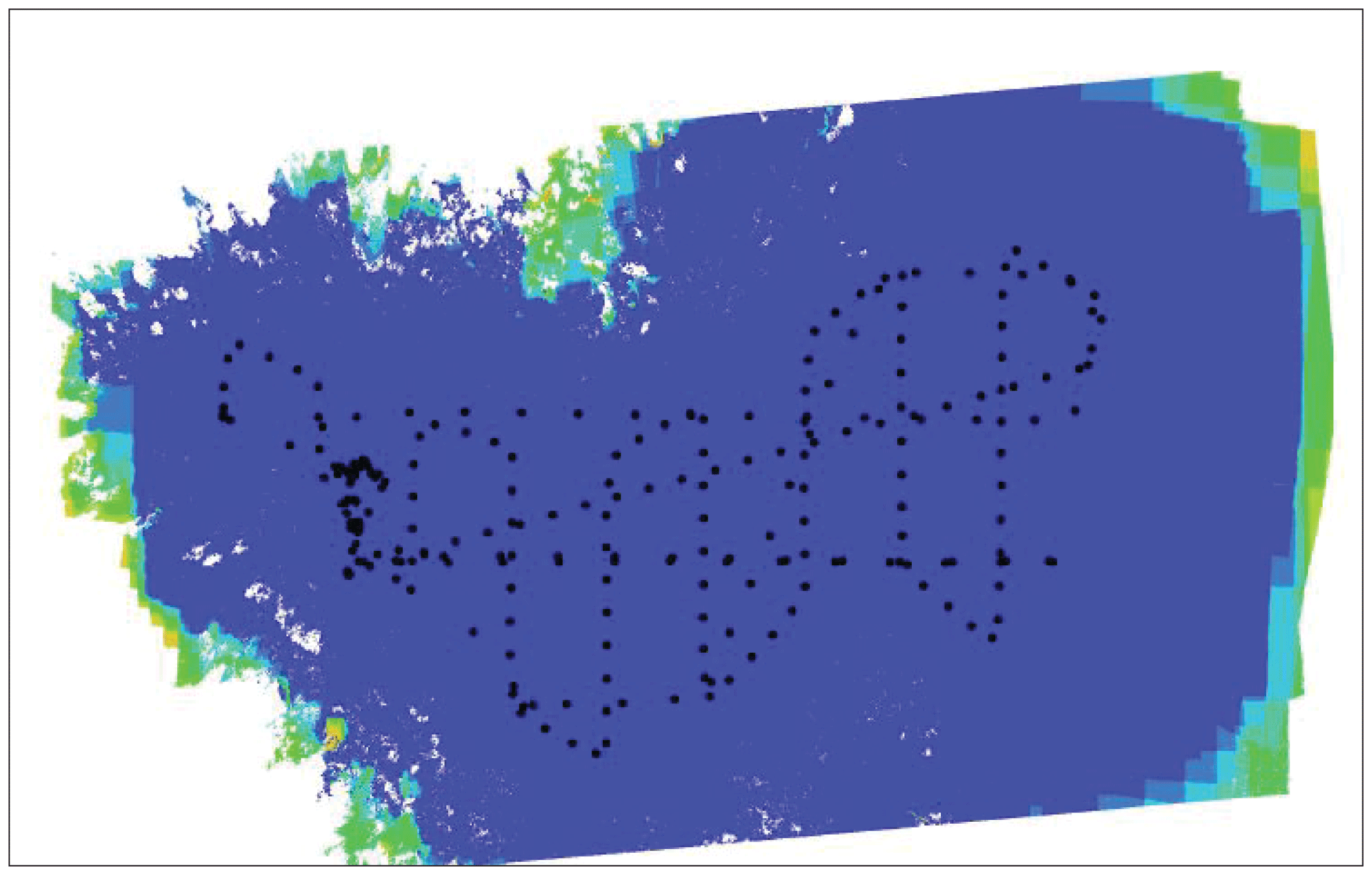
Flight pattern (dots) and image (blue) frames generated for experimental uncrewed aircraft systems flight in Granby, Colorado.
In the processing, we used only 4 GCPs and about 72,000 automatically generated tie points. The selection of tie points is discussed further in the next section because tie points are essential for calibration.
Data Acquisition Flight Patterns
Collecting data using an orthogonal flight pattern may offer the best means to maximize the accuracy of the data for a given number of GCPs because the tie points used for completing camera calibration/interior orientation parameter determination are imaged multiple times and are at different sections of the camera frame, which leads to a more robust least-squares solution to the interior orientation parameters used in the extended collinearity equations.
Geometric Calibration
Camera calibration aims to describe the path of a ray of light that enters a camera at the time of exposure. The parameters used to completely characterize this process are termed the interior orientation parameters. The main parameters are the focal length of the lens and the location of the principal point of symmetry; however, for photogrammetric purposes, the knowledge of the deviation of the light ray from a straight line, described by polynomial coefficients, also is important. This deviation is termed lens distortion, and the polynomial coefficients are termed lens distortion parameters. In this research, two methods used by the USGS are presented to determine these parameters for small and medium format digital cameras.
The importance of calibrating a camera used for photogrammetric purposes cannot be overstated. Although it is possible to obtain accurate orthoproducts without a well calibrated camera, these products would require a dense network of control points. Such a network will make a photogrammetric project prohibitively expensive. The calibration procedures described in this research are based on the least-squares solution to the photogrammetric resection problem. The projective collinearity equations form the basis for the mathematical model.
wherex, y
are the measured image coordinates of a feature,
xp, yp
are the locations of the principle point of the lens in the image coordinate system,
f
is the focal length, and
is the camera orientation matrix.
Because the lens in the camera is a complex system consisting of a series of lenses, the path of light is not always rectilinear. The result is that a straight line in object space is not imaged as one in the image. The effect is termed distortion. Primarily, we are interested in characterizing the radial distortion and decentering distortion. Radial (Miller and others, 2020) distortion displaces the image points along the radial direction from the principal point (Mugnier and others, 2004). The distortion also is symmetrical around the principal point. The distortion is defined by a polynomial (Brown, 1971; Light, 1992):
where The (x, y) components of the radial distortion are given by the following equation:The second type of distortion is the decentering distortion, which is due to the displacement of the principle point from the center of the lens system. The distortion has radial and tangential components and is asymmetrical with respect to the principal point (Mugnier and others, 2004). The components of decentering distortion, in the x-y direction, are given by δx2=P1(r2+2x2)+2P2xy and δy2=2P1xy+P2(r2+2y2).
A third distortion element, specific to digital cameras, accounting for scale distortion of pixel sizes in the x-y direction also is incorporated:
The final mathematical model is a result of adding all the equations to the right-hand side of the collinearity equations to obtain the following “extended collinearity equations.”
Laboratory-Based Methods
The USGS EROS Center hosted a digital camera calibration facility that could be replicated at NUPO. The position of the calibration cage, with respect to the room, is shown in figure 8. For longer focal length cameras, a large room is required; however, for the UAS camera, the room should be large enough to hold the cage and have about 3 m of space in front of the cage to hold a tripod. Some of the positions for locating the cameras are shown in figure 8. The cage consists of three parallel panels. Each panel has several circular retroreflective targets (dots) and a few coded targets (fig. 9). The coded targets are so referred because the pattern of the placement of the individual circular dots that make up these targets is unique (fig. 10). Each coded target has five dots that are positioned in the same relative orientation as the red lines shown in figure 10. The intersection of the red lines is taken as the center of the coded target. For the calibration procedure, the camera lens is always focused at infinity. The choice of the distance of the camera from the front panel of the cage depends on the focal length of the camera and the depth of focus that has been selected. Once the camera-cage distance is fixed, three angular positions from the center of the front panel of the cage are selected. The angular positions are selected with the optimal angles for convergent photography in mind, within the limitation of the dimensions of the calibration room. Ideally, the angular positions will be close to the positions shown in figure 8.
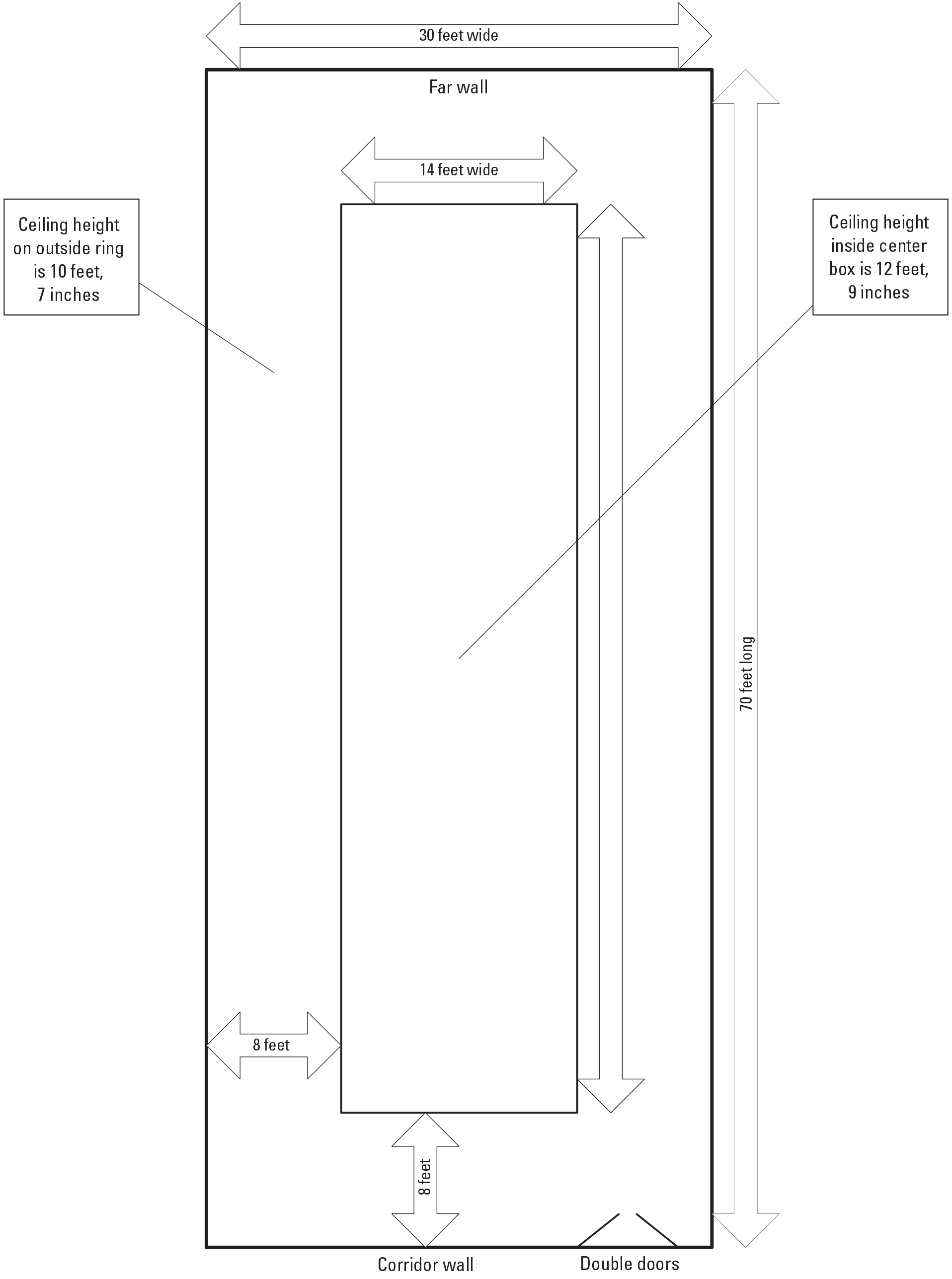
Layout of the calibration laboratory and the calibration cage.
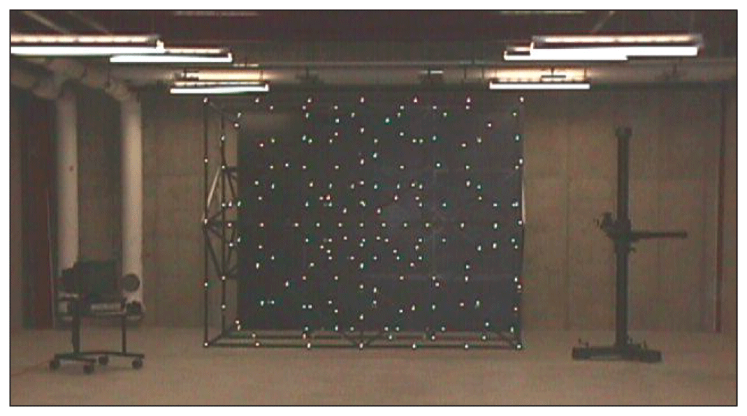
Photograph of the calibration cage.
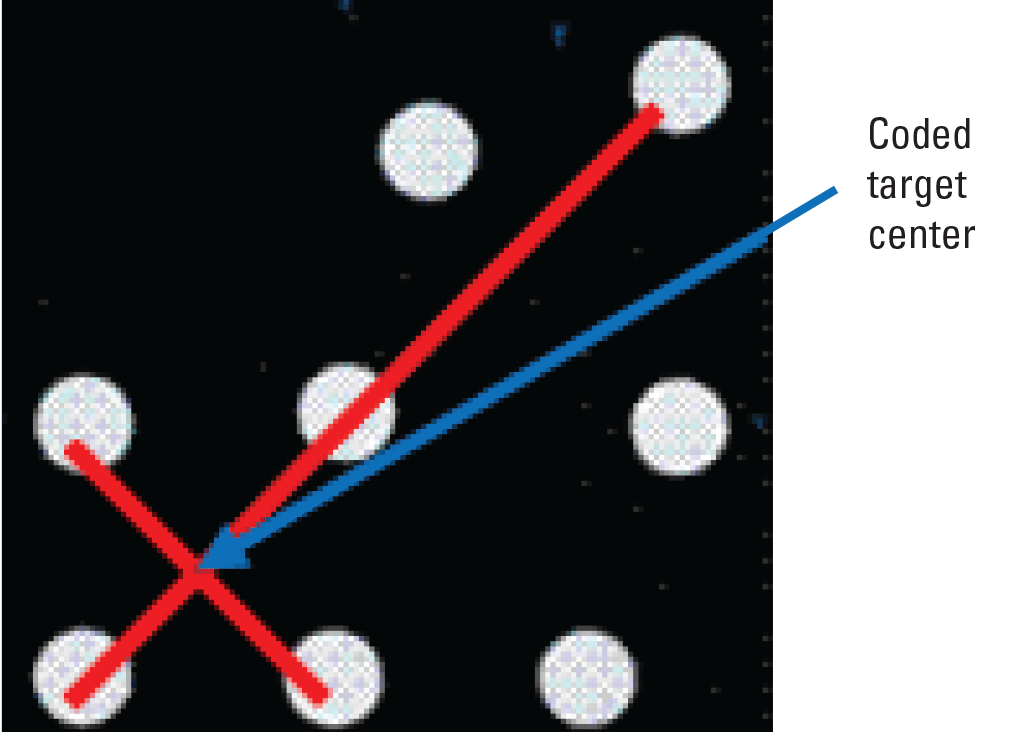
Five dots (connected with red lines) that make up the pattern in a coded target.
Once the images are captured, they can be processed using software called Australis (Fraser 1997). Australis uses a free network method of bundle adjustment. The software recognizes the patterns in the coded targets and calculates their center. The coded target center is not the actual centroid of the individual target dots but is determined in a manner shown in figure 10. The software requires at least four coded targets in each image that are common with other images and uses the targets to determine the initial relative orientation of the camera at all the exposure stations. The software then uses the circular targets to determine a free network least-squares bundle adjustment solution of the extended collinearity equations. Because it is a free network solution, the least-squares iteration converges easily, and a relative measure of the geometry of the system (the lens, camera, and targets) is obtained.
The USGS used to operate a multicollimator calibration instrument at Reston, Virginia, from 1973 to 2019 (Light, 1992). The instrument was used to calibrate film-based cameras, and although digital cameras are increasingly used, several photogrammetric companies still use film cameras. The aerial camera is placed on top of the collimator bank, aligned, and focused at infinity. Images that capture the precision targets in telescope lenses (of the multicollimator) are taken. The deviation of the measured image (x, y) coordinates from the known (X, Y) coordinates forms the basis for solving for the calibration parameters.
A simple procedure for completing in situ calibration is to use a chess board pattern and the vertices squares as the calibration target device. This method has been developed by the California Institute of Technology (Bouguet, 2022). This procedure may be useful in featureless areas where obtaining enough tie points to get good calibration parameters is difficult or areas where establishing ground control is difficult. The goal would be to complete calibration before flight (similar to the radiometric calibration of targets).
Laboratory/In Situ Calibration Using Dense Ground Control Points
Many metric camera manufacturers use in situ methods of calibration in conjunction with laboratory-based calibration methods to produce the best camera calibration results. These methods are mostly used for calibrating large cameras that cannot be easily calibrated in laboratories alone. The cameras are hence calibrated while they are in operation and fixed to the aerial platform. In situ calibration methods require an area (a calibration range) with a dense distribution of highly accurate control points. While maintaining a high density, the control points in the calibration range should be well distributed in the horizontal and vertical directions. A rigorous least-squares block adjustment based on the colinearity equations augmented by equations modeling radial and decentering distortion can generate accurate calibration parameters. The in situ method requires aerial imagery over a calibration range, which can be inconvenient to the camera operators. Also, careful maintenance of the calibration range is required.
In Situ Field-Based Self-Calibration Using Dense Tie Points and Sparse Ground Control Points
In theory, laboratory-based calibration offers the most accurate possibilities to calibrate the UAS camera. In practice, laboratory-based geometric calibration is considered impractical for calibrating UAS sensors, often because calibration parameters can change between laboratory and field because the sensors are not stable.
The field-based self-calibration method combines the best of laboratory- and field-based calibration methods. This method uses a sparse set of GCPs and combines them with automatically extracted tie points from the imagery data collected during acquisition. This method is the most common method in UAS-based mapping. This process determines the calibration parameters as part of the overall data (3D point cloud, orthophotograph mosaic, digital elevation model, and so on) generation process; for example, in the Agisoft Metashape software. Methods of self-calibration include generating Kruppa equations (Faugeras and others, 1992), enforcing linear constraints on the calibration matrix (Hartley, 1994), a method that determines the absolute quadric, which is the image of the cone at a plane at infinity. Although many techniques are used by researchers (Faugeras and others, 1992; Hartley, 1994), most of these techniques do not find solutions for distortion and principal point because they are not considered critical for computer vision. On the other hand, for photogrammetrists, these are critical parameters necessary to produce an accurate product at a moderate price.
Ideally, UAS cameras can be calibrated with a combination of field and laboratory testing. The initial interior orientation parameters may be obtained from the laboratory tests, and these parameters can be refined in the field; however, the USGS has many researchers and several hundred camera sensors in use. An in situ calibration during data acquisition is probably best suited. UAS data processing software can allow researchers to calibrate the camera using data collected during the data acquisition process.
Most structure from motion software completes self-calibration using image matching techniques by automatically identifying conjugate “tie” points across multiple images. Self-calibration (in Agisoft, this is the alignment stage) combines interior orientation and camera (optical) distortion parameter estimation with exterior orientation (the position and orientation of the sensor at the time of photography) estimation. The self-calibration (internal to the software) happens in the “pixel domain or dimension”; that is, the size of the pixel is the basic measurement, and all the interior orientation parameters (focal length, principal point location, and distortion parameters) are determined in that dimension and converted to “distance units” internally by multiplying the values with the physical size of the pixel. Often, using GCPs at this stage constrains this (nonlinear) problem, limits the overall errors, and ensures that final data products match the GCP locations. The calibration parameters thus obtained are always optimized to the data (and the GCPs), which is preferred. To ensure data are of acceptable quality in other locations, one must ensure that the tie points are well distributed, vertically and horizontally, which may require breaking up the project or processing boundaries in accordance with the terrain. It is generally noted that the accuracy of the orthoimage is high and may be a direct function of the accuracy of GCPs used for the project. The vertical accuracy often depends on the terrain (for correlation) and the geometry. Although the geometry of data collection imposes enough constraints to limit horizontal errors, vertical measurements may not have enough constraints (see fig. 11). This also is the case with global positioning system-based measurements where horizontal accuracy is 2–3 times better than vertical accuracy.
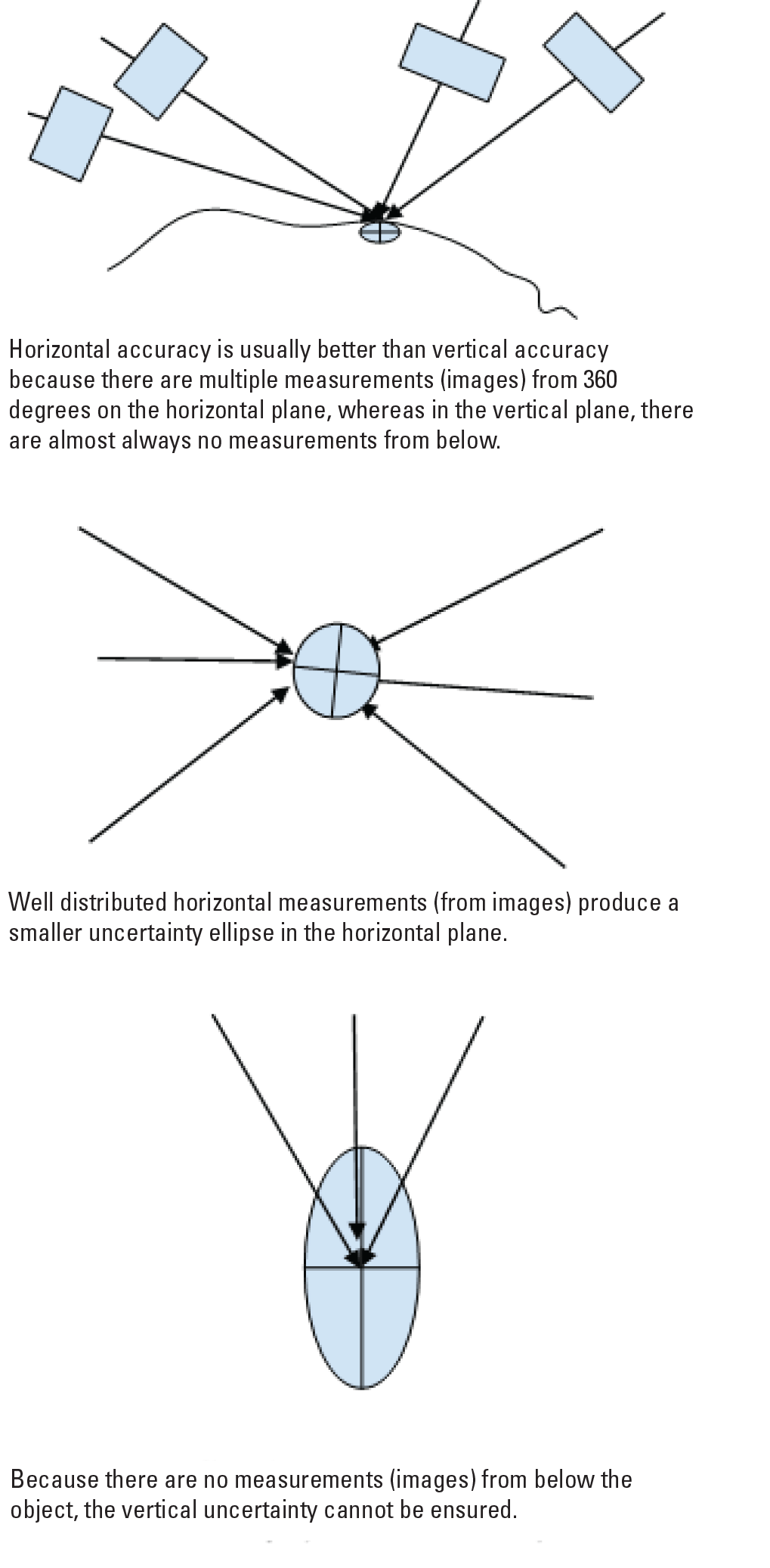
Satellite positions used to ensure accuracy in measurements and structure from motion data.
The automatically detected tie points used for calibration and the spatial distribution of GCPs are important to the stability of the calibration parameters; therefore, it is recommended that tie points be chosen to represent stable surfaces (as opposed to treetops, leaves, and so on). This method of choosing tie points may be achievable if the reprojection accuracy requirements of tie points are chosen appropriately, along with a requirement that the tie points are imaged from at least six locations, to ensure (depending on the overlap and side lap percentage) that tie points are imaged from opposing flight lines.
Data Quality Control
The American Society for Photogrammetry and Remote Sensing positional accuracy standards for geospatial data indicate that at least 30 GCPs be used to assess the positional accuracy of any geospatial data (American Society for Photogrammetry and Remote Sensing, 2014). The requirement follows the Federal Geographic Data Committee standards (Federal Geographic Data Committee, 1998) and is based on decades of experience with aerial photogrammetric orthoimagery products. For USGS researchers, collection of 30 signalized or photograph-identifiable GCPs is the recommended practice when possible.
A screenshot from the Agisoft Metashape software, where GCPs can be selected for use in calibrating the cameras used for data acquisition, is shown in figure 12. The calibration routine needs to be run multiple times, and in each run (or trial), a subset of GCPs and all the automatically generated tie points could be used to generate calibration parameters. The rest of the GCPs (those not used) become validation points for that trial. At each iteration, the residuals against these “check points” are stored. After several trials (typically at least 30), the residuals are summarized. These cross-validated residuals can provide an accurate summary of the accuracy of data, even when the American Society for Photogrammetry and Remote Sensing and Federal Geographic Data Committee recommended number of control points are not available.
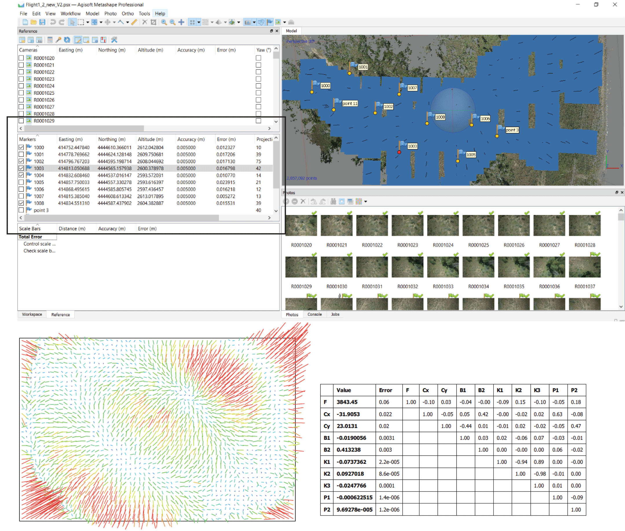
Agisoft Metashape software generating calibration parameters using cross validation.
The method uses a random subset of GCPs to generate a residual/coefficient pair. Using multiple random pairs can generate an optimal set of calibration parameters and allow independent data validation. GCPs should be well distributed in the planimetric dimension and the elevation dimension. The accuracy of GCPs determines the quality of data whereas the accuracy of check points determines how well the data can be validated. In general, the remote sensing data cannot be more accurate than the GCPs; therefore, the method of measurement of GCPs is important. In most cases, real-time kinematic solutions-based GCPs offer an accuracy of around 2–3 cm at 1 sigma, which indicates that the accuracy of UAS imagery can be validated only to as much as 6 cm. Where higher accuracy is desired, researchers could use total station methods for measuring GCPs.
Additional Calibration Considerations
Additional considerations for calibration are described in this section. These include calibration targets, thermal band calibration, test ranges, optimal flight patterns, cross validation to reduce GCP requirements, in situ geometric calibration, and metadata.
Calibration Targets
Calibration accuracy of the UAS image using the ELM depends on the number and quality of calibration panels used during a field campaign. Some of the commercial high-quality reflectance targets are expensive. A calibration target provided commercially may be smaller in size and might not provide enough pure pixels for radiometric calibration of UAS; therefore, calibration panel options that are cost-effective, large enough to provide 10 by 10 pure pixels, and lightweight enough to deploy during a UAS field campaign would be beneficial.
House siding material has been used previously (Wang and Myint, 2015); however, this material is not lightweight. An alternative that could be investigated is the use of canvas, which is lightweight and comes in a variety of colors, including black, dark gray, and gray. Canvas can be dyed or painted to suit the individual campaign criteria and is easily portable. A lightweight plastic or wood frame needs to be designed and tested. A canvas that is slightly larger than 1 square meter would be ideal. Velcro applied to the edge of the canvas for attachment to the frame would allow for complete stretching of the canvas across the frame. Tent spikes could be used to hold the canvas and frame in place in the field. A bubble level would ensure the canvas target was horizontal. A complete characterization of the canvas panel could be completed using spectroradiometer. Additionally, the target reflectance could be acquired in the field and laboratory. Degradation patterns could be characterized by leaving the canvas in the Sun over several days, making hourly spectroradiometer measurements. Other materials also could be considered. For example, lightweight resins molded by a 3D printer could be evaluated in the same way and secured to the ground using tent spikes. Developing lightweight, Lambertian, reflectance-stable targets continues to be of interest in the remote sensing community. Human-made targets would offer better control over spectral reflectance and surface characteristics than natural targets.
Thermal Band Calibration
The fundamental idea of the UAS thermal band calibration also is similar to the solar reflective band calibration. However, thermal band calibration has more challenges because it requires the calibration target to demonstrate a stable temperature throughout the field campaign. Additionally, the temperature of the target would need to be monitored throughout the campaign; therefore, deployment of a thermal radiometer would be necessary.
The “cold” target requirement can be easily achieved using an ice/water bath in a plastic tote. The plastic tote provides little thermal signature, and the presence of ice and water ensures the mixture is at a triple point; therefore, it demonstrates a known temperature of 0 degrees Celsius reliably. Use of a large plastic tote for a reasonably sized target is ideal for achieving the 10 x 10 pure pixel criterion mentioned previously. The warm target is more difficult to achieve. A black lid on the plastic tote could be used to absorb solar radiation, and field tests could determine if a stable maximum temperature is achieved or elusive. In either case, a thermal radiometer could be used to measure the temperature of the black lid coincident with the UAS fly over. Laboratory-based calibration indicates that thermal radiometer instruments are accurate to within 1.28 kelvins (Miller and others, 2020). The DN and temperature measurement of thermal calibration targets from the UAS image and thermal radiometer, respectively, can be used to establish the empirical relation between the targets. A set of calibration coefficients obtained from the empirical relation can be used to calibrate the remaining UAS pixels.
Developing Test Ranges
Sensors can be assessed using a test grid of GCPs on a test range to be established by EROS in consultation with NUPO. Researchers at EROS would need to work with NUPO to establish a test range of GCPs to assess new sensors, which may include structure from motion (camera), thermal, and lidar sensor specific targets. Another option is to assess these sensors by completing extensive surveys during UAS data collection.
Investigating Optimal Flight Patterns
The optimized flight pattern can be assessed for maximizing accuracy. A limited set of experiments has been completed; however, they were not completed on a standard test range. Testing ideally would include collecting data by flying aircraft at two elevations, and the second flight elevation should be 50 percent higher than the first and at cross directions.
Cross Validation to Reduce Ground Check Point Requirements
A limited set of experiments has been completed on a single dataset; however, the process requires automatic processing using computer programming, which has not been completed yet. The process estimates error by completing calibration multiple times. While completing calibration/alignment steps using GCPs, it is recommended to use a random subset of GCPs and complete/refine calibration of the sensor using this subset. This step can be repeated multiple times (by computer programming; each time selecting a different random set of GCPs for calibration), completing verification (error assessment) on the points not used for calibration each time (Hastie and others, 2009). Finally, the residual values of errors in the GCPs not used at each trial can be summarized for error estimation.
In Situ Geometric Calibration for Optimal Calibration
In situ geometric calibration may be especially useful in featureless areas where it is difficult to get enough tie points to get good calibration parameters or areas where it is difficult to establish ground control. The goal would be to complete calibration before flight. One possible method to investigate could be the chess board calibration pattern developed by the California Institute of Technology (Bouguet, 2022).
Metadata
Metadata are important in providing the users of data with all the calibration information necessary to make UAS data and products useful. Metadata also provide the basis for the assessment of data quality and the possibility of data sharing and comparing between scientists.
Study of metadata based on the following broad classes may be continued in the following areas:
-
• Pixel specific metadata.
-
• Signal-to-noise ratio.
-
• Radiometric resolution (gives an indication of the quality of a pixel value stored in a data product).
-
• Measurement time (to reconstruct the Sun’s position).
-
• Illumination conditions.
-
• Storing measurement geometry of the field of view or the instantaneous field of view of every pixel, for imaging sensors.
-
-
• Scene-based metadata.
Metadata can be stored in Material Template Library files, having uncertainty assigned to quantitative metadata parameters. Additional factors to consider that were not visible in remote sensing data of coarser resolution, for example, include wind and wind gusts that can affect the spectral signature.
Conclusions
The calibration procedures described in this document range from simple to complex; however, using any of these procedures can improve the usability of UAS data. Calibration procedures bring the UAS remote sensing data to a common unit of measurement and are quantifiable and comparable with other data.
By using two well characterized reflectance panels and acquiring site measurements in a standardized manner, globally digestible data can be collected. Because ELM for calibration is sensor independent, sensor calibration activities (that is, sending the sensor out for certified third-party analysis) are unnecessary. Most importantly, a globally useful set of calibrated images is produced, which could not be achieved through sensor calibration in this venue. The results are immediate in that image-calibrated remote sensing data are analysis ready for multiple parties with minimal, if any, format modifications, which could shorten the time required to publish findings.
Using an orthogonal flight pattern to collect data can maximize the accuracy of data for a given number of GCPs because the tie points used for completing camera calibration/interior orientation parameter determination are imaged multiple times and are at different sections of the camera frame, which leads to a more robust least-squares solution to the interior orientation parameters used in the extended collinearity equations.
A simple procedure for completing in situ calibration is to use a chess board pattern and the vertices squares as the calibration target device. This method has been developed by the California Institute of Technology (Bouguet, 2022). This procedure may be especially useful in featureless areas where it is difficult to get enough tie points to get good calibration parameters or areas where it is difficult to establish ground control. The goal would be to complete calibration before flight.
The automatically detected tie points used for calibration and the spatial distribution of GCPs are important to the stability of the calibration parameters; therefore, it is recommended that tie points be chosen to represent stable surfaces (as opposed to treetops, leaves, and so on). This method of choosing tie points may be achievable if the reprojection accuracy requirements of toe points are chosen appropriately, along with a requirement that the tie points are imaged from at least six locations, which help ensure (depending on the overlap and side lap percentage) that tie points are imaged from opposing flight lines.
GCPs should be well distributed in the planimetric dimension and the elevation dimension. The accuracy of GCPs determines the quality of data whereas the accuracy of check points determines how well the data can be validated. In general, the remote sensing data cannot be more accurate than the GCPs; therefore, the method of measurement of GCPs is important. In most cases, real-time kinematic solutions-based GCPs offer an accuracy of around 2–3 cm at 1 sigma, which indicates that the accuracy of UAS imagery can be validated only to as much as 6 cm. If higher accuracy is desired, the researchers may want to consider using total station based methods for measuring GCPs.
The development of a calibration and validation test site containing targeted and “natural” control and check points can aid in developing and verifying innovative data acquisition and processing techniques and validation of final data products. Finally, the metadata should include all calibration coefficients and documented processes used in generating the data, including any links to theoretical basis documents, calibration coefficient parameters, and GCPs.
Acknowledgments
This report documents the research efforts of the U.S. Geological Survey Earth Resources Observation and Science Center and the National Unmanned Aircraft Systems Project Office. Many of the requirements for calibration and validation of data have been gleaned from interviews with U.S. Geological Survey uncrewed aircraft systems researchers, including Matthew Burgess, Dr. Dennis Helder, Sandy Brosnahan, Dr. Christopher Holmquist-Johnson, Josip Adams, Mark Bauer, Todd Preston, and David Wood.
References Cited
American Society for Photogrammetry and Remote Sensing, 2014, ASPRS positional accuracy standards for digital geospatial data: American Society for Photogrammetry and Remote Sensing, v. 81, no. 3, p. A1–A26, accessed March 2023 at https://doi.org/10.14358/PERS.81.3.A1-A26.
Ben-Dor, E., Kruse, F.A., Lefkoff, A.B., and Banin, A., 1994, Comparison of three calibration techniques for utilization of GER 63-channel aircraft scanner data of Makhtesh Ramon, Negev, Israel: Photogrammetric Engineering and Remote Sensing, v. 60, no. 11, p. 1339–1354. [Also available at https://www.infona.pl/resource/bwmeta1.element.elsevier-0cf033ad-9ecd-3951-98af-780ae4bfeae1.]
Bouguet, J.-Y., 2022, Camera calibration toolbox for Matlab (1.0): CaltechDATA digital data, accessed March 2023 at https://doi.org/10.22002/D1.20164.
Brown, D.C., 1971, Close-range camera calibration: Photogrammetric Engineering, v. 37, no. 8, p. 855–866. [Also available at https://www.asprs.org/wp-content/uploads/pers/1971journal/aug/1971_aug_855-866.pdf.]
Doctor, K.Z., Bachmann, C.M., Gray, D.J., Montes, M.J., and Fusina, R.A., 2015, Wavelength dependence of the bidirectional reflectance distribution function (BRDF) of beach sands: Applied Optics, v. 54, no. 31, p. F243–F255. [Also available at https://doi.org/10.1364/AO.54.00F243.]
Dunford, R., Michel, K., Gagnage, M., Piégay, H., and Trémelo, M.-L., 2009, Potential and constraints of unmanned aerial vehicle technology for the characterization of Mediterranean riparian forest: International Journal of Remote Sensing, v. 30, no. 19, p. 4915–4935. [Also available at https://doi.org/10.1080/01431160903023025.]
Dwyer, J.L., Kruse, F.A., and Lefkoff, A.B., 1995, Effects of empirical versus model-based reflectance calibration on automated analysis of imaging spectrometer data—A case study from the Drum Mountains, Utah: Photogrammetric Engineering and Remote Sensing, v. 61, no. 10, p. 1247–1254. [Also available at https://www.asprs.org/wp-content/uploads/pers/1995journal/oct/1995_oct_1247-1254.pdf.]
Farhad, M.M., Kaewmanee, M., Leigh, L., and Helder, D., 2020, Radiometric cross calibration and validation using 4 angle BRDF model between Landsat 8 and Sentinel 2A: Remote Sensing (Basel), v. 12, no. 5, art. 806, 20 p., accessed March 14, 2023, at https://doi.org/10.3390/rs12050806.
Farrand, W.H., Singer, R.B., and Merényi, E., 1994, Retrieval of apparent surface reflectance from AVIRIS data—A comparison of empirical line, radiative transfer, and spectral mixture methods: Remote Sensing of Environment, v. 47, no. 3, p. 311–321. [Also available at https://doi.org/10.1016/0034-4257(94)90099-X.]
Faugeras, O.D., Luong, Q.-T., and Maybank, S.J., 1992, Camera self-calibration—Theory and experiments, in Sandini, G., ed., Lecture notes in computer science (v. 588): Margherita Ligure, Italy, Springer-Verlag, p. 321–334. [Also available at https://doi.org/10.1007/3-540-55426-2_37.]
Fawcett, D., and Anderson, K., 2019, Investigating impacts of calibration methodology and irradiance variations on lightweight drone-based sensor derived surface reflectance products, in Neale, C.M.U., and Maltese, A., eds., Remote sensing for agriculture, ecosystems, and hydrology XXI (proceedings of SPIE, v. 11149), Strasbourg, France, September 9–11, 2019: Strasbourg, France, SPIE, 14 p. [Also available at https://doi.org/10.1117/12.2533106.]
Ferrier, G., and Wadge, G., 1996, The application of imaging spectrometry data to mapping alteration zones associated with gold mineralization in southern Spain: International Journal of Remote Sensing, v. 17, no. 2, p. 331–350. [Also available at https://doi.org/10.1080/01431169608949009.]
Fraser, C.S., 1997, Digital camera self-calibration: ISPRS Journal of Photogrammetry and Remote Sensing, v. 52, no. 4, p. 149–159. [Also available at https://doi.org/10.1016/S0924-2716(97)00005-1.]
Freemantle, J., Pu, R., and Miller, J., 1992, Calibration of imaging spectrometer data to reflectance using pseudo-invariant features, in Proceedings of the Fifteenth Canadian Symposium on Remote Sensing, Toronto, Ontario, Canada, June 1–4, 1992: North York, Ontario, Canada, Ontario Centre for Remote Sensing, p. 452–455.
Gevaert, C.M., Suomalainen, J., Tang, J., and Kooistra, L., 2015, Generation of spectral–temporal response surfaces by combining multispectral satellite and hyperspectral UAV imagery for precision agriculture applications: IEEE Journal of Selected Topics in Applied Earth Observations and Remote Sensing, v. 8, no. 6, p. 3140–3146. [Also available at https://doi.org/10.1109/JSTARS.2015.2406339.]
Goldman, D.B., 2010, Vignette and exposure calibration and compensation: IEEE Transactions on Pattern Analysis and Machine Intelligence, v. 32, no. 12, p. 2276–2288. [Also available at https://doi.org/10.1109/TPAMI.2010.55.]
Han-Ya, I., Ishii, K., and Noguchi, N., 2010, Satellite and aerial remote sensing for production estimates and crop assessment: Environment Control in Biology, v. 48, no. 2, p. 51–58. [Also available at https://doi.org/10.2525/ecb.48.51.]
Hartley, R.I., 1994, Euclidean reconstruction from uncalibrated views, in Mundy, J.L., Zisserman, A., and Forsyth, D., eds., Applications of invariance in computer vision: Ponta Delgada, Azores, Portugal, Springer, p. 235–256. [Also available at https://doi.org/10.1007/3-540-58240-1_13.]
Hastie, T., Tibshirani, R., and Friedman, J., 2009, The elements of statistical learning—Data mining, inference, and prediction (2d ed.): New York, Springer Science & Business Media, 745 p. [Also available at https://hastie.su.domains/Papers/ESLII.pdf.]
Helder, D., Markham, B., Morfitt, R., Storey, J., Barsi, J., Gascon, F., Clerc, S., LaFrance, B., Masek, J., Roy, D.P., Lewis, A., and Pahlevan, N., 2018, Observations and recommendations for the calibration of Landsat 8 OLI and Sentinel 2 MSI for improved data interoperability: Remote Sensing (Basel), v. 10, no. 9, art. 1340, 29 p., accessed March 14, 2023, at https://doi.org/10.3390/rs10091340.
Helder, D., Thome, K.J., Mishra, N., Chander, G., Xiong, X., Angal, A., and Choi, T., 2013, Absolute radiometric calibration of Landsat using a pseudo invariant calibration site: IEEE Transactions on Geoscience and Remote Sensing, v. 51, no. 3, p. 1360–1369. [Also available at https://doi.org/10.1109/TGRS.2013.2243738.]
Iqbal, F., Lucieer, A., and Barry, K., 2018, Simplified radiometric calibration for UAS-mounted multispectral sensor: European Journal of Remote Sensing, v. 51, no. 1, p. 301–313. [Also available at https://doi.org/10.1080/22797254.2018.1432293.]
Jackson, R.D., Clarke, T.R., and Moran, M.S., 1992, Bidirectional calibration results for 11 spectralon and 16 BaSO4 reference reflectance panels: Remote Sensing of Environment, v. 40, no. 3, p. 231–239. [Also available at https://doi.org/10.1016/0034-4257(92)90005-5.]
Joseph, W., Aerts, S., Vandenbossche, M., Thielens, A., and Martens, L., 2016, Drone based measurement system for radiofrequency exposure assessment: Bioelectromagnetics, v. 37, no. 3, p. 195–199. [Also available at https://doi.org/10.1002/bem.21964.]
Kelcey, J., and Lucieer, A., 2012, Sensor correction and radiometric calibration of a 6-band multispectral imaging sensor for UAV remote sensing: International Archives of the Photogrammetry, Remote Sensing and Spatial Information Sciences, v. XXXIX–B1, p. 393–98. [Also available at https://doi.org/10.5194/isprsarchives-XXXIX-B1-393-2012.]
Kruse, F.A., Kierein-Young, K.S., and Boardman, J.W., 1990, Mineral mapping at Cuprite, Nevada with a 63-channel imaging spectrometer: Photogrammetric Engineering and Remote Sensing, v. 56, no. 1, p. 83–92. [Also available at https://www.asprs.org/wp-content/uploads/pers/1990journal/jan/1990_jan_83-92.pdf.]
Laliberte, A.S., Goforth, M.A., Steele, C.M., and Rango, A., 2011, Multispectral remote sensing from unmanned aircraft—Image processing workflows and applications for rangeland environments: Remote Sensing (Basel), v. 3, no. 11, p. 2529–2551. [Also available at https://doi.org/10.3390/rs3112529.]
Lee, Y., Park, E.-T., Jeong, J., Shi, H., Kim, J., Kang, B.-S., and Song, W., 2020, Weight optimization of hydrogen storage vessels for quadcopter UAV using genetic algorithm: International Journal of Hydrogen Energy, v. 45, no. 58, p. 33939–33947. [Also available at https://doi.org/10.1016/j.ijhydene.2020.09.014.]
Light, D.L., 1992, The new camera calibration system at the U.S. Geological Survey: Photogrammetric Engineering and Remote Sensing, v. 58, no. 2, p. 185–188. [Also available at https://www.asprs.org/wp-content/uploads/pers/1992journal/feb/1992_feb_185-188.pdf.]
Mamaghani, B.G., and Salvaggio, C., 2019, Comparative study of panel and panelless-based reflectance conversion techniques for agricultural remote sensing: American Journal of Agricultural Science, v. 6, no. 4, p. 40–58. [Also available at https://home.cis.rit.edu/~cnspci/references/mamaghani2019b.pdf.]
Mansouri, A., Marzani, F., and Gouton, P., 2005, Development of a protocol for CCD calibration—Application to a multispectral imaging system: International Journal of Robotics and Automation, v. 20, no. 2, p. 94–100. [Also available at https://doi.org/10.2316/Journal.206.2005.2.206-2784.]
McArdle, S., Miller, J., and Freemantle, J., 1992, Airborne image acquisition under cloud—Preliminary comparisons with clear-sky scene radiance and reflectance imagery, in Proceedings of the Fifteenth Canadian Symposium on Remote Sensing, Toronto, Ontario, Canada, June 1–4, 1992: Toronto, Ontario, Canada, Ontario Centre for Remote Sensing, p. 446–449.
MicaSense, 2022, Radiometric calibration mode for MicaSense sensors: MicaSense web page, accessed April 27, 2022, at https://support.micasense.com/hc/en-us/articles/115000351194-Rededge-Camera-Radiometric-Calibration-Model.
Miller, J., Gerace, A., Eon, R., Montanaro, M., Kremens, R., and Wehle, J., 2020, Low-cost radiometer for Landsat land surface temperature validation: Remote Sensing, v. 12, no. 3, art. 416, 13 p., accessed March 14, 2022, at https://doi.org/10.3390/rs12030416.
Pajares, G., 2015, Overview and current status of remote sensing applications based on unmanned aerial vehicles (UAVs): Photogrammetric Engineering and Remote Sensing, v. 81, no. 4, p. 281–330. [Also available at https://doi.org/10.14358/PERS.81.4.281.]
Pro-Lite Technology, Ltd., 2022, Welcome to Pro-Lite: Pro-Lite Technology, Ltd., web page, accessed April 9, 2020, at https://www.pro-lite.co.uk/File/spectralon_targets.php.
Rango, A., Laliberte, A.S., Herrick, J.E., Winters, C., Havstad, K.M., Steele, C., and Browning, D.M., 2009, Unmanned aerial vehicle-based remote sensing for rangeland assessment, monitoring, and management: Journal of Applied Remote Sensing, v. 3, no. 1, art. 033542, 19 p. [Also available at https://doi.org/10.1117/1.3216822.]
Roy, D.P., Zhang, H.K., Ju, J., Gomez-Dans, J.L., Lewis, P.E., Schaaf, C.B., Sun, Q., Li, J., Huang, H., and Kovalskyy, V., 2016, A general method to normalize Landsat reflectance data to nadir BRDF adjusted reflectance: Remote Sensing of Environment, v. 176, p. 255–271. [Also available at https://doi.org/10.1016/j.rse.2016.01.023.]
Sarkar, M., Büttgen, B., and Theuwissen, A.J.P., 2013, Feedforward effect in standard CMOS pinned photodiodes: IEEE Transactions on Electron Devices, v. 60, no. 3, p. 1154–1161. [Also available at https://doi.org/10.1109/TED.2013.2238675.]
Smith, G.M., and Milton, E.J., 1999, The use of the empirical line method to calibrate remotely sensed data to reflectance: International Journal of Remote Sensing, v. 20, no. 13, p. 2653–2662. [Also available at https://doi.org/10.1080/014311699211994.]
Toth, C., and Jóźków, G., 2016, Remote sensing platforms and sensors—A survey: ISPRS Journal of Photogrammetry and Remote Sensing, v. 115, p. 22–36. [Also available at https://doi.org/10.1016/j.isprsjprs.2015.10.004.]
Wang, C., and Myint, S.W., 2015, A simplified empirical line method of radiometric calibration for small unmanned aircraft systems-based remote sensing: IEEE Journal of Selected Topics in Applied Earth Observations and Remote Sensing, v. 8, no. 5, p. 1876–1885. [Also available at https://doi.org/10.1109/JSTARS.2015.2422716.]
Wu, A., Xiong, X., Cao, C., and Angal, A., 2008, Monitoring MODIS calibration stability of visible and near-IR bands from observed top-of-atmosphere BRDF-normalized reflectances over Libyan Desert and Antarctic surfaces, in Butler, J.J., and Xiong, J., eds., Earth observing systems XIII (proceedings of SPIE, v. 7081), San Diego, Calif., August 10–14, 438 p.
Yu, W., 2004, Practical anti-vignetting methods for digital cameras: IEEE Transactions on Consumer Electronics, v. 50, no. 4, p. 975–983. [Also available at https://doi.org/10.1109/TCE.2004.1362487.]
Zhu, Y.T., Lowe, T.C., and Langdon, T.G., 2004, Performance and applications of nanostructured materials produced by severe plastic deformation: Scripta Materialia, v. 51, no. 8, p. 825–830. [Also available at https://doi.org/10.1016/j.scriptamat.2004.05.006.]
Conversion Factors
Abbreviations
BRDF
bidirectional reflectance distribution function
DN
digital number
DOI
Department of the Interior
ELM
empirical line method
EROS
Earth Resources Observation and Science
GCP
ground control point
GNSS
global navigation satellite system
GSD
ground sample distance
NUPO
National Unmanned Aircraft Systems Project Office
QA
quality assurance
QC
quality control
UAS
uncrewed aircraft systems
USGS
U.S. Geological Survey
3D
three dimensional
°
degree
For more information about this publication, contact:
Director, USGS Earth Resources Observation and Science Center
47914 252nd Street
Sioux Falls, SD 57198
605–594–6151
For additional information, visit: https://www.usgs.gov/centers/eros
Publishing support provided by the
Rolla and Sacramento Publishing Service Centers
Disclaimers
Any use of trade, firm, or product names is for descriptive purposes only and does not imply endorsement by the U.S. Government.
Although this information product, for the most part, is in the public domain, it also may contain copyrighted materials as noted in the text. Permission to reproduce copyrighted items must be secured from the copyright owner.
Suggested Citation
Sampath, A., Shrestha, M., While, M., and Scholl, V.M., 2023, Guidelines for calibration of uncrewed aircraft systems imagery: U.S. Geological Survey Open-File Report 2023–1033, 23 p., https://doi.org/10.3133/ofr20231033.
ISSN: 2331-1258 (online)
| Publication type | Report |
|---|---|
| Publication Subtype | USGS Numbered Series |
| Title | Guidelines for calibration of uncrewed aircraft systems imagery |
| Series title | Open-File Report |
| Series number | 2023-1033 |
| DOI | 10.3133/ofr20231033 |
| Publication Date | July 25, 2023 |
| Year Published | 2023 |
| Language | English |
| Publisher | U.S. Geological Survey |
| Publisher location | Reston, VA |
| Contributing office(s) | Earth Resources Observation and Science (EROS) Center |
| Description | v, 23 p. |
| Online Only (Y/N) | Y |