

Learning from a High-Severity Fire Event: Conditions Following the 2018 Carr Fire at Whiskeytown National Recreation Area
Links
- Document: Report (16 MB pdf) , HTML , XML
- Data Releases:
- USGS Data Release - UAS imagery at Whiskeytown National Recreation Area in 2018 and 2019 following the Carr Fire
- USGS Data Release - Forest conditions following the 2018 Carr Fire at Whiskeytown National Recreation Area
- NGMDB Index Page: National Geologic Map Database Index Page (html)
- Download citation as: RIS | Dublin Core
Acknowledgments
We thank the U.S. National Park Service (NPS) and U.S. Geological Survey crews who collected data; C. Freeman and K. Mosher for unoccupied aircraft system data acquisition, planning, logistics, and analysis; and L. Shaskey and additional NPS staff for providing key logistical support for fieldwork. The NPS Klamath Inventory and Monitoring program supplied field data. This manuscript was funded by the U.S. Geological Survey Ecosystems Mission Area to the Western Ecological Research Center, H.R. 2157; Additional Supplemental Appropriations for Disaster Relief Act 2019 (Public Law 116-20); and the U.S. National Park Service (IAA P18PG00450 and P19PG00287).
Abstract
The 2018 Carr Fire burned more than 90 percent of Whiskeytown National Recreation Area, with much of the park burning at high severity. California yellow pine and mixed conifer forests are not well adapted to large, high-severity fires, and forest recovery after these events may be problematic. Large, high-severity fire patches pose difficulties for recruitment with interiors that are long distances from potential seed trees and may develop fuel structures that can promote further high-severity fire. This report details patterns of forest structure derived from field plots measured 2–3 years after the Carr Fire, providing a characterization of immediate fire effects. We coupled these observations with remotely sensed information, including data collected from unoccupied aircraft system surveys. The remotely sensed data were used to depict erosion after the Carr Fire as well as to create a high-resolution land cover classification map, a debris flow risk map and hazard assessment, and a post-fire canopy vegetation loss map. Results indicated high levels of tree mortality after the Carr Fire, including high-value old growth forest stands, supporting remotely sensed assessments of fire severity. The high-resolution tree mortality model also aligned well with other remotely sensed estimates of immediate burn severity. Results of the land cover classification illustrated the high percentage of dead vegetation remaining in the understory and canopy 8 months post-fire. Changes in vegetation height identified areas with canopy vegetation loss from 1- to 8-months post-fire. Pairing the post-fire debris accumulation with debris flow probabilities may identify high-risk debris flow areas. The results of this study will help inform future decisions concerning wildland fire and vegetation management strategies at Whiskeytown National Recreation Area and are broadly relevant for management in the aftermath of large, high-severity fires in mixed, dry coniferous forests in the western United States.
Introduction
The 2018 Carr Fire burned more than 90 percent of Whiskeytown National Recreation Area (WHIS). Much of the coniferous forests at WHIS burned at high severity, killing many of the large, overstory trees (fig. 1). The National Park Service (NPS) faces several challenges developing a path forward for park management after the Carr Fire and other high-severity fires (for example, the 2021 Dixie Fire and KNP Complex Fire). Successfully navigating these challenges is made easier by gaining a detailed picture of immediate fire effects and an outlook for forest recovery in moderate- and high-severity fire patches.
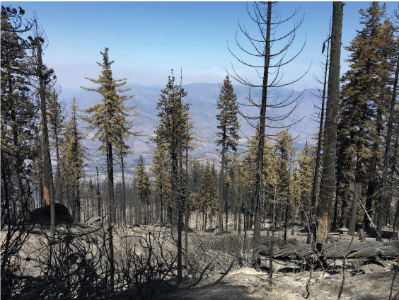
Mixed conifer forest conditions immediately following high-severity fire at Upper Boulder Creek, Whiskeytown National Recreation Area. Photograph by Eamon Engber, National Park Service.
The objective of this study is to describe the immediate effects of the Carr Fire, with a particular emphasis on the conifer forests at WHIS. The Carr Fire provides a potential preview of expected fire behavior and forest responses in an era of increasing “megadisturbances” (Millar and Stephenson, 2015). Managers will need to develop new insights, strategies, and tools to facilitate forest adaptation to these changing conditions. These approaches are primarily centered on increasing disturbance resistance (remaining unchanged in the face of disturbance), resilience (promoting forest recovery to pre-disturbance composition or structure), and managing transitions to more stable vegetation communities (Holling, 1973; Folke and others, 2004; Petraitis, 2013). Describing immediate fire effects helps managers decide which of these strategies is appropriate and where to effectively deploy each one.
In cooperation with the U.S. National Park Service (NPS), this research considered the effects of the 2018 Carr Fire, focusing on understanding patterns of mortality (resistance) and regeneration (resilience) in post-fire conifer forests at WHIS to inform future management decisions following large, high-severity fires in mixed dry coniferous forests in the western United States. Specifically, we seek to answer these questions:
-
• How has conifer forest structure changed in long-term and temporary forest monitoring sites at WHIS after the Carr Fire?
-
• How were old-growth conifer forest stands affected by the Carr Fire?
-
• Can intensive unoccupied aircraft system (UAS) surveys be used to assess the effects of fire on forest cover and structure?
Methods
Study Area
WHIS is situated in the southeast part of the Klamath Mountains in northern California (fig. 2). WHIS experiences a Mediterranean climate, with hot, dry summers and cool, wet winters. At low elevations at WHIS, the average annual temperature is 14 degrees Celsius (°C) with annual precipitation of 152 centimeters (cm; U.S. Department of Interior, 2003), though the climate varies sharply over the mountainous terrain at WHIS. The vegetation at WHIS also varies with elevation (Smith and others, 2021). Vegetation at relatively low elevation is composed of shrub and oak species, primarily California black oak (Quercus kelloggii Newb.), canyon live oak (Quercus chrysolepis Liebm.), and tanoak (Notholithocarpus densiflorus (Hook. & Arn.) Manos, C.H. Cannon & S. Oh). Low to mid-elevations also contain knobcone pine (Pinus attenuata Lemmon), gray pine (P. sabiniana Douglas), and yellow pine (Pinus jeffreyi Grev. & Balf. and P. ponderosa Douglas ex Lawson & C. Lawson). Mixed conifer forests are found at higher elevations, often dominated by white fir (Abies concolor (Gordon & Glend.) Lindl. ex Hildebr.) and Douglas-fir (Pseudotsuga menziesii (Mirb.) Franco). The highest elevation forests at WHIS are comprised of red fir (Abies magnifica A. Murray bis). There was intensive logging in the 1950s and 1960s across much of the yellow pine and mixed conifer forests at WHIS before the park was established.
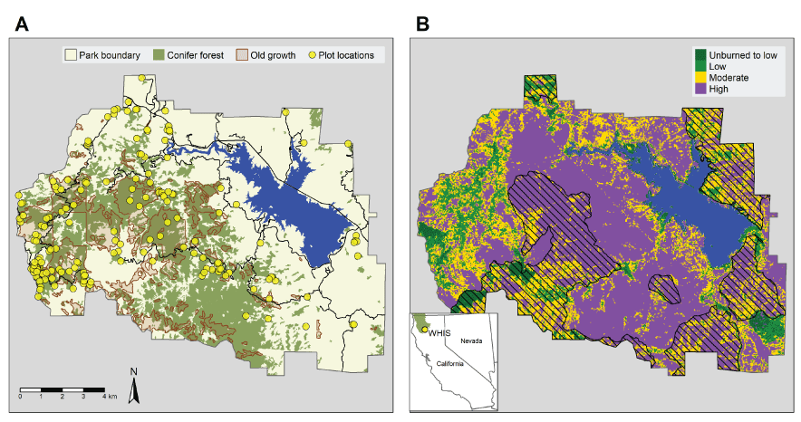
Simplified vegetation types and location of existing plot-based vegetation survey data at Whiskeytown National Recreation Area (WHIS). A, Assessments of fire severity following the Carr Fire using data from Monitoring Trends in Burn Severity (Monitoring Trends in Burn Severity, https://www.mtbs.gov); and B, the hashed areas show footprints from earlier wildfires. The inset shows the location of WHIS (yellow circle) within the Klamath region (in green) in Northern California.
Fire was historically common in the many coniferous forests across western North America, with fire return intervals in mixed-conifer forests at WHIS generally less than 5 years before 1850 (Fry and Stephens, 2006). Indigenous burning practices were halted by the arrival of Europeans in the mid-19th century, whereas other land uses, such as intensive logging and grazing, further altered these landscapes (Hagmann and others, 2021). Fire suppression policies effectively removed fire from these landscapes for much of the 20th century (Stephens and Ruth, 2005), including at WHIS (Fry and Stephens, 2006). The net result of these changes was the accumulation of surface fuel and the establishment of small trees and shrubs, which allow fire to readily move from the surface to forest canopies (Skinner, 1995; Taylor, 2000). This general pattern was also present at WHIS, where Leonzo and Keyes (2010) reported a cohort of small shade-tolerant tree species that could allow surface fire to reach forest canopies, increasing the potential for high-severity fire.
In response to these changes, the National Park Service began a program of fuel treatments in the mid-1990s, which used mechanical treatments (thinning and mastication) and prescribed fire to reduce fuel and fire hazards. Within the past decades there have been several wildfires at WHIS, most notably the 2008 Moon Fire (part of the Shasta-Trinity Unit Lightning Complex Fire). The Carr Fire started in late July 2018 at WHIS. On July 26, 2018, weather, topography, and fuel combined to produce rapid fire spread, including a fire vortex that had windspeeds greater than 64 meters per second (Lareau and others, 2018). The Carr Fire eventually burned more than 90,000 hectares (ha), causing 7 fatalities and the destruction of more than 1,500 structures (https://www.fire.ca.gov/incidents/2018/7/23/carr-fire/).
Post-fire Severity Patterns
We used several separate plot-based data sources to determine site-level changes in forest structure, which allowed us to capitalize on existing long-term plot data collected before and after the fire to reliably infer fire-caused changes. We also collected additional post-fire plot data to increase the coverage of these data sources. In the following section, we describe each of these plot-based data sources.
National Park Service Plots
Fine-scale assessments of forest condition were obtained using a combination of remeasuring existing plots and by installing new plots. The NPS installed plots using three different protocols, described in this report.
Before the Carr Fire, managers at WHIS installed more than 40 0.1-ha forest monitoring plots following protocols in the NPS Fire Monitoring Handbook (FMH; https://www.nps.gov/orgs/1965/upload/fire-effects-monitoring-handbook.pdf). Typically, these plots were established prior to fuel management treatments to document forest and fuel structure. These plots were revisited multiple times before the Carr Fire. In 2019, the NPS resurveyed most of these plots for forest structure, and seedling density was surveyed in 2019 and 2020. Standard procedures for the FMH plots include recording stem diameter at breast height (DBH; 1.37 m), species identity, and live and dead status for all trees greater than 15-centimeters (cm) DBH (National Park Service, 2003). Additional measurements of live tree saplings (stems greater than or equal to 2.5 to less than or equal to 15-cm DBH) were collected in a 0.025 ha subplot within each plot.
The NPS also installed plots to monitor thinning treatment effectiveness in black oak/ponderosa pine and canyon live oak forest types in the Boulder and Brandy Creek treatment units. There were 10 plots installed in each unit. The Brandy Creek plots were installed in 2010, and the Boulder Creek plots were installed in 2013. Plots within each treatment unit were remeasured several times before the Carr fire and again after the fire in 2019. The plot design differed from FMH plots, described earlier. Species identity, live and dead status, and DBH were measured for overstory trees (more than 28-cm DBH) within a 15 m (0.071 ha) radial plot, whereas saplings (from 2.5 to 28 cm) were measured in 8 m (0.020 ha) radial subplots.
We used available plot data from the Klamath Inventory and Monitoring (I&M) Program at WHIS. The Klamath I&M plots at WHIS are part of a long-term effort to determine vegetation changes at national parks in northern California and southern Oregon (Smith and others, 2021). The Klamath I&M Program surveys vegetation at randomly located sites stratified across vegetation types in the park, with trees (stems greater than or equal to 15-cm DBH) inventoried at 0.1-ha plots and saplings (stems greater than 2.5 to less than 15-cm DBH) inventoried in four 10-square meter subplots. At each sampling occasion, observations on trees for species identity, size, and condition (including live/dead status) are recorded, whereas live saplings are tallied in the subplots. Details on the vegetation sampling are presented in Odion and others (2011). We used 46 Klamath I&M plots that had pre- and post-Carr Fire surveys. Most plots were inventoried in WHIS in 2018 just before to the Carr Fire (one plot was inventoried in 2012; seven plots were inventoried in 2015) and inventoried again in 2022 (post-fire).
Temporary Plots
In addition to the NPS data, we established 108 temporary plots in the summers of 2020 and 2021 (fig. 2). For most of these plots (n=76), we used Geographic Information Systems to randomly select sampling locations within conifer forests conditioned on locations with slopes less than or equal to 50 percent, being greater than 50 m and less than 500 m from a road, and greater than or equal to 100 m from non-vegetated areas (for example, Whiskeytown lake). The sampling locations were stratified across burn severity and predicted conifer regeneration. Monitoring Trends in Burn Severity (MTBS) data were unavailable when we generated the samples, so burn severity was derived using the National Burn Severity Mapping Project extended severity assessment (https://burnseverity.cr.usgs.gov), whereas conifer regeneration was predicted using the models developed in Stewart and others (2021) and the poscrptR R package (Wright and others, 2020). We used a vegetation alliance map (National Park Service, https://irma.nps.gov/DataStore/Reference/Profile/2233415) to identify conifer forests by selecting polygons with Douglas-fir, mixed conifer, ponderosa pine, or red fir forest alliance types. We established 12 of the 108 plots within UAS sampling polygons (described later in the text) to assist with future vegetation mapping projects using the same criteria described earlier, with the exception that plot locations were stratified by burn severity and whether the forest alliance was conifer (described earlier in the text) or oak, including black oak, blue oak, canyon live oak, interior live oak, Oregon white oak, and tanoak forest and woodland alliances. We established 20 of the 108 temporary plots in the same locations as earlier surveys of old-growth conifer forests (Leonzo and Keyes, 2010). Three of the original plot locations described in Leonzo and Keyes (2010) could not be reached because of unsafe conditions, so we located three replacement plots using the same plot location criteria outlined in Leonzo and Keyes (2010). Where possible, we measured sampling point locations with high locational precision, collecting at least 50 Global Positioning System (GPS) positions for each point, which were averaged and adjusted using post-processing differential correction. Note that for 31 of the 108 plots, we collected locations with a lower precision handheld GPS. At each sampling point, we measured slope, aspect, and visually estimated fuel (Scott and Burgan, 2005). Forest plots covered a range of forest types and burn severities (fig. 2).
At the temporary plots, we measured live and standing dead trees, recording stem diameter at breast height, species identity, and live and dead status for all trees greater than 15-cm DBH over a 0.1-ha circular plot. Within a 0.011-ha subplot at the plot center, we measured sapling (stems from 0.1- to 15.0-cm DBH) stem diameter, species location, and status. We measured distance and azimuth to the plot center for all overstory trees within the UAS plots.
We estimated the difference between pre- and post-fire forest conditions in all plot types by summarizing stand density and basal area for overstory trees and saplings in six major genera: (1) Abies, (2) Pinus, (3) Calocedrus, (4) Pseudotsuga, (5) Quercus, and (6) Notholithocarpus. Because no pre-fire observations were available for the temporary plots, we summarized post-fire observations by status (live and dead), assuming that dead trees are a rough proxy for fire related mortality. We compared pre- and post-fire and live and dead stand structure summaries by burn severity, using data from MTBS (https://www.mtbs.gov/). Data used in these analyses (including old growth forest structure, see the “Changes in Old Growth Forest Structure” section) can be found in a data release by Wright and others (2024).
Changes in Old Growth Forest Structure
We used a 35.56-cm diameter threshold similar to that used in Leonzo and Keyes (2010) to classify old growth trees for all plots (temporary, FMH, and I&M) located in old growth areas, as determined using the same NPS timber type map (National Park Service, unpublished data, 2010) as Leonzo and Keyes (2010). Leonzo and Keyes (2010) used visual cues to further classify old growth trees; we did not. We compared the total number of plots by burn severity class for each plot type as well as the proportion of dead old growth post-Carr Fire basal area. We also calculated the proportion of dead basal area (out of total) using the original data for all of the resampled plots (n=17) from Leonzo and Keyes (2010). We compared this proportion against the proportion of dead basal area from the 2020 and 2021 samples in the same plots.
Remotely Sensed Data
Plot-based surveys provide fine-scale estimates of forest conditions that are usually limited in scale, and therefore, we incorporated remotely sensed data to assess larger areas in WHIS. We related the plot data (described earlier) to landscape-scale products and metrics based on lidar (light detection and ranging) and UAS (orthoimagery and multispectral sensor) imagery. Lidar is a method of 3D mapping by measuring distances between a sensor and surface with a returning laser signal. Terrestrial lidar penetrates vegetation and provides high-resolution images of the Earth’s surface. The existing lidar data covering the park boundary consists of acquisitions from 2011 to 2019. The lidar data were viewed in conjunction with available imagery, including normalized difference vegetation index (NDVI, measure of vegetation greenness). UAS data are processed to create 3D structures from 2D images based on the theory and techniques of structure-from-motion photogrammetry (Ullman, 1979; Westoby and others, 2012; Fonstad and others, 2013). Although UAS multispectral sensors do not penetrate vegetation, the 3D point cloud structures it produces are often comparable to that of lidar ground mapping. UAS survey areas were identified by the Burned Area Emergency Response (BAER) program and NPS teams as areas with high potential for post-fire erosion and debris flows. Also, locations with cultural resources and severe burn effects were identified and surveyed with UAS.
Unoccupied aircraft system flights used a 3DR Solo quadcopter platform (3DR Robotics) with a Ricoh GR II camera (www.ricoh-imaging.co.jp/english/products/gr-2/) for high resolution (3.4 cm at 400 feet [ft] above ground level [AGL] horizontal resolution) orthoimagery and a MicaSense RedEdge (www.ageagle.com/solutions/micasense-series-multispectral-cameras/) multispectral sensor (8 cm at 400 feet [ft] AGL horizontal resolution). UASs were flown at 400-ft AGL with both sensors. Multiple ground control points were deployed and surveyed using a Real time kinematic GPS. Photogrammetry was conducted in Metashape (Agisoft LLC, 2021) to produce orthoimagery, elevation models, and surface models. The orthoimagery data were used to create digital elevation models (DEM) for 2019 surveys and digital surface models (DSM) for 2018 and 2019 surveys. The multispectral sensor provided an 8-cm resolution layer that was used as the basis for an NDVI analysis of forest plots and burned areas. NDVI is an important metric to assess forest burned, unburned, and revegetation extent as well as recovery progress (table 1).
Table 1.
Name and description of all spectral vegetation indices and elevation models used in analyses.[NIR, near infrared band; Red, red band; —, no data]
UAS surveys with both sensors were completed in October 2018 (fig. 3) immediately after the fire, which provided a baseline dataset for post-fire effects on elevation change and vegetation. These baseline areas were resurveyed in May 2019 with the Ricoh sensor and in June 2019 with the MicaSense sensor. The 2018 UAS flights used an adjacent parallel transect pattern (lawnmower) for data collection, whereas in 2019, a crosshatch pattern was used to reduce data gaps by flying overlapping perpendicular flight paths. Additional UAS flights were planned for 2020 but were cancelled because of the grounding of the U.S. Department of the Interior UAS fleet. The UAS datasets were analyzed to determine if any erosion or canopy vegetation loss occurred between the 2018 and 2019 surveys. Further, the high-resolution multispectral imagery was used to classify post-fire land cover.
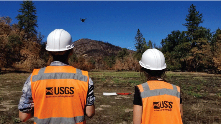
U.S. Geological Survey employees conducting unoccupied aircraft system (UAS) surveys at Whiskeytown National Recreation Area, October 2018. Photograph by the U.S. Geological Survey.
Land-cover Classification
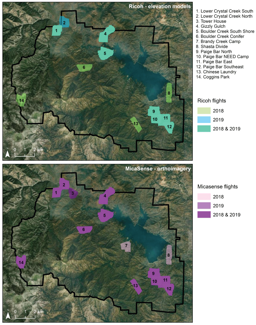
High-resolution multispectral imagery from the May/June 2019 UAS flights were used to calculate spectral vegetation indices and elevation models (table 1). Seven WHIS sites had data from both sensors (MicaSense and Ricoh) in 2019 (Lower Crystal Creek North, Grizzly Gulch, Boulder Creek South Shore, Paige Bar East, Paige Bar NEED Camp, Paige Bar North, and Paige Bar Southeast). Training polygons were manually generated, and values were extracted from vegetation and elevation layers to train the random forest model and classify site images into 10 land cover groups: (1) bare ground, (2) dead grass/understory, (3) dead trees/shrubs, (4) infrastructure, (5) pavement, (6) rock, (7) water, (8) grass, (9) trees (greater than 8 meters [m]), and (10) shrubs (less than 8 m). Not enough live trees remained to classify trees further into group or species using this classification method. The random forest model included additive predictors: MicaSense bands (blue, green, red edge), NDVI, Modified Soil Adjusted Vegetation Index (MSAVI), Chlorophyll Index Red Edge (CIRE), DEM, DSM, and Canopy Height Model (CHM; table 1).
Erosion and Debris Flow Risk Assessment
Change in ground elevation (DEMs) from fall 2018 to spring 2019 was calculated to determine if erosion was detectable (table 2). Change in vegetation height also was calculated to determine canopy vegetation loss and to identify areas of potential debris accumulation following fire containment (table 2). Elevation models were resampled at 1 m to account for minor pixel variability between flight pattern differences by year (lawnmower versus crosshatch). Canopy height loss was grouped into three categories (5–10 m, 10–20 m, and 20+ m) and mapped with the Carr Fire’s Post Wildfire Debris Flow Hazard Assessment (U.S. Geological Survey, 2022). This assessment estimated percent probability of debris flow at stream segments given a designed high-intensity, short-duration rainstorm (15-minute peak intensity of 24 millimeters per hour), which has triggered debris flows at USGS monitoring sites in other burn areas and is likely to happen in most western states (U.S. Geological Survey, 2022). The combination of our high-resolution vegetation change measurements with existing moderate-resolution debris flow risk models may provide managers with valuable information on habitat change and risk after high-severity wildfires. Data for the remotely sensed information can be found in a data release by Thorne and others (2024).
Table 2.
Remote sensing analyses with corresponding flight sensor files, sites, and descriptions.[DEM, digital elevation model; NA, not applicable; DSM, digital surface model; CHM, canopy height model]
Results
Post-fire Severity Patterns
National Park Service Plots
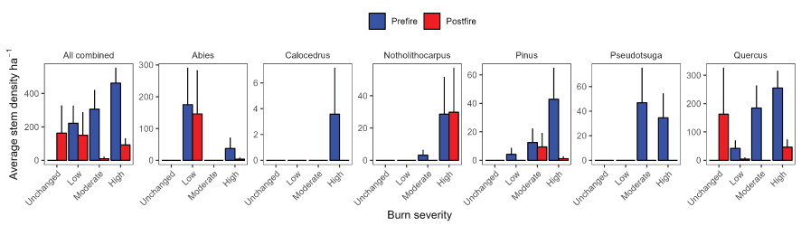
We detected a steep decline in average live tree basal area and stem density with increasing fire severity in the FMH plots (fig. 4). This trend was especially apparent in the sapling size class (less than or equal to 15-cm DBH), where nearly all live trees died except in the unchanged burn severity class (fig. 5). We found similar patterns in the Boulder and Brandy Creek plots (figs. 6, 7). However, the Boulder and Brandy Creek plots did have some notable differences. Unlike the FMH plots, there was little difference in mortality patterns in plots that burned at moderate and high severity, and saplings in the plots that burned at low severity showed less dramatic changes than occurred in the FMH plots.
Average pre- and post-fire live basal area and stem density (±1 standard error) for overstory trees (diameter at breast height greater than 15 centimeters) in the Fire Monitoring Handbook plots. Data are shown for all trees and selected genera by burn severity class.
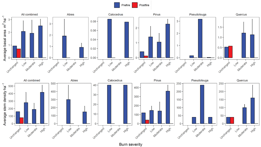
Average pre- and post-fire live basal area and stem density (plus or minus 1 standard error) for saplings (diameter at breast height greater than 2.5 centimeters [cm] and less than or equal to 15 cm) in Fire Monitoring Handbook plots. Data are shown for all trees and selected genera by burn severity classes.
Average pre- and post-fire live basal area and stem density (plus or minus 1 standard error) for overstory trees (diameter at breast height greater than 15 centimeters) in the Boulder and Brandy Creek plots. Data are shown for all trees and select genera by burn severity classes.
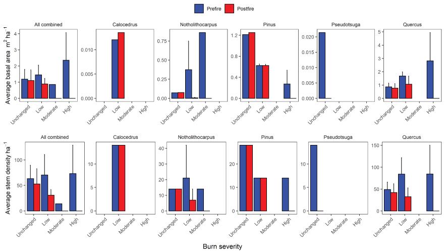
Average pre- and post-fire live basal area and stem density (plus or minus 1 standard error) for saplings (diameter at breast height greater than 2.5 centimeters [cm] and less than or equal to 15 cm) in the Boulder and Brandy Creek plots. Data are shown for all trees and select genera by burn severity classes.
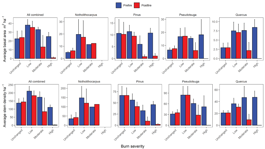
The Klamath I&M plots showed similar patterns as the other NPS plots following the Carr Fire (figs. 8, 9). Average basal area and stem density of trees declined in most sites, particularly for areas that experienced moderate to high severity fire. Changes were less apparent for plots that were in the unchanged and low burn severity classes. Similar to trees, saplings in the Klamath I&M plots had sharp declines in stem densities following the Carr Fire across most genera and burn severity classes. Stem diameter for saplings was not measured in the Klamath I&M plots, so we were unable to calculate changes in basal area for stems in this size class for these plots.
Average pre- and post-fire live basal area and stem density (plus or minus 1 standard error) for overstory trees (diameter at breast height greater than or equal to 15 centimeters) in the Klamath Inventory and Monitoring plots. Data are shown for all trees and select genera by burn severity classes.
Average pre- and post-fire live stem density (plus or minus 1 standard error) for pole size trees (diameter at breast height less than 2.5 centimeters [cm] and greater than 15 cm) in the Klamath Inventory and Monitoring Creek plots. Data are shown for all trees and select genera across observed Normalized Difference Burn Ratio classes.
Overall, the dramatic changes between pre- and post-fire basal area and stem density for standing trees within moderate- and high-severity classes indicates that these plots experienced substantial tree mortality after the Carr Fire, although changes in sapling density was less apparent in two resprouting hardwood genera, Notholithocarpus and Quercus.
Temporary Plots
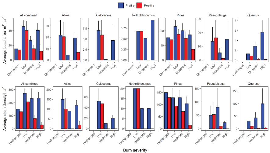
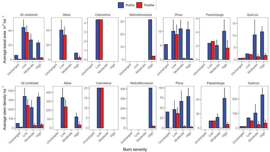
The average dead basal area of overstory trees in the temporary plots increased with increasing burn severity, whereas average live basal area tended to decrease (fig. 10). This pattern was mirrored in tree density. Average dead sapling basal area was higher than average live sapling basal area in nearly all cases (fig. 11). However, differences between live and dead trees with increasing burn severity were less apparent for sapling density in some genera, particularly for Notholithocarpus and Quercus. The similarity between live and dead stem density for these genera was largely because of what seemed to be basal resprouts in high-severity plots.
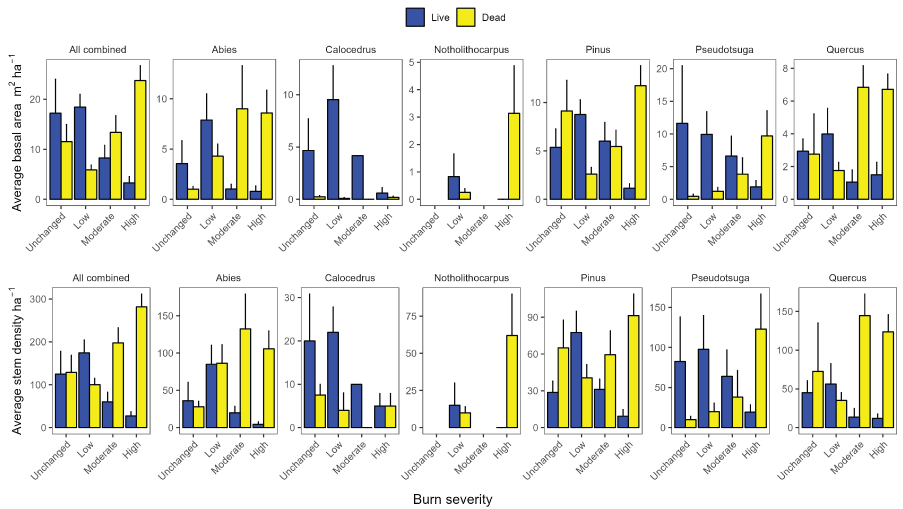
Average live and dead basal area and stem density (plus or minus 1 standard error) for overstory trees (diameter breast height greater than 15 centimeters) in the temporary plots. Data are shown for all trees and select genera by burn severity classes.
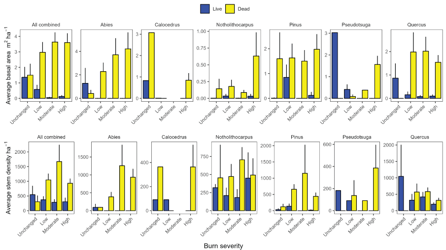
Average live and dead basal area and stem density (plus or minus 1 standard error) for saplings (diameter breast height greater than or equal to 0.1 centimeter [cm] and less than or equal to 15 cm) in the temporary plots. Data are shown for all trees and select genera by burn severity classes.
Changes in Old Growth Forest Structure
More than half of the old growth area in the Carr fire burned at high severity. With the exception of a single plot, the proportion of dead basal area in the 2020 and 2021 post-fire sample dwarfed the values recorded in 2006 (Leonzo and Keyes, 2010; fig. 12). Plot F3 had a lower proportion of dead basal area in the post-fire sample, which was unexpected. However, Leonzo and Keyes (2010) recorded that this plot had a large number of snags, some of which might have fallen in the intervening years or were consumed during the Carr Fire. This plot also burned at low severity with relatively little overstory tree mortality, providing few opportunities to replace any fallen dead trees.
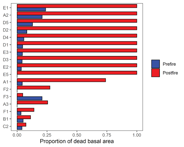
Proportion of dead basal area for pre- and post-fire measurements of the Leonzo and Keyes (2010) plot locations (plot identifier on y-axis). Pre-fire measurements were recorded in 2006; post-fire measurements were recorded in 2020 and 2021.
It should be noted that the Leonzo and Keyes (2010) plots disproportionately burned at high severity. Out of the 17 resampled Leonzo and Keyes plots, 12 (71 percent) burned at high severity according the MTBS assessments (fig. 13). In contrast, just over half of the other plot types located in the old growth areas burned at high severity and suffered much less proportional basal area loss.
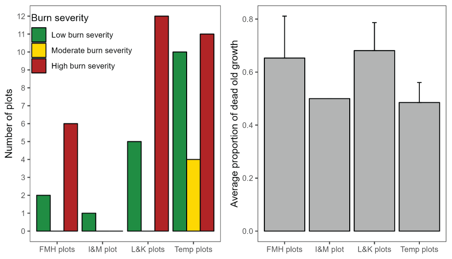
Number of plots by burn severity class and proportion of old dead growth (plus or minus 1 standard error) by plot type for all plots in old growth areas. Old growth areas were determined using an unpublished timber type map from the National Park Service. Old growth trees were defined using the diameter threshold listed in Leonzo and Keyes (2010). Axis labels for Leonzo and Keyes (2010) plots are abbreviated to “L&K plots,” and temporary plots are labeled “Temp plots.” Only a single inventory and monitoring plot with post-fire data was in an old growth area; it is labeled “I&M plot.”
Remotely Sensed Data
UAS surveys were completed in fall 2018 and spring 2019 across 14 sites and covered a total of 1,092 ha (fig. 14). In 2018, a total of 61 flights were conducted (approximately 13 hours of flight time), and in 2019, 87 flights were conducted (approximately 17 hours of flight time) for elevation surveys using the Ricoh sensor. The DEMs and DSMs generated from UAS data from late fall 2018 and spring 2019 were compared to determine if erosion or debris flows could be detected. Only three sites (Brandy Creek Campground, Coggins Park, and Shasta Divide Dozer Line) have DSMs because of processing issues with DEM construction (fig. 14). A qualitative comparison of the DEMs did not reveal any areas that experienced large-scale erosion (fig. 15) of management concern. However, a quantitative estimate of elevation change was not possible because of inherent differences in surveying methods between the two periods; the 2018 survey used a lawnmower style flight path, whereas the 2019 survey used a crosshatch flight path. Additionally, there were substantial foliage remaining on the burned trees during the 2018 survey, which had fallen from the trees by the 2019 survey and created a mismatch in bare ground overlap. Structure from motion techniques can only capture what is visible from the air and are not capable of penetrating vegetation. We investigated elevation differences over two static landscape features (a dirt road and a parking area) to better understand the effects of the different surveying methods (lawnmower versus crosshatch). We detected median elevation differences of 1.39 m across the road and 0.28 m across the parking area. Elevation differences across open landscapes were minor and equally variable. Despite the issues in comparing the DEMs, the data from 2019 serve as a high-resolution baseline of elevation and vegetation cover for future assessments of forest recovery (fig. 16; appendix 1).
Location of unoccupied aircraft system surveys across Whiskeytown National Recreation Area. A total of 1,092 hectares was flown in fall 2018 and spring 2019. Locations were selected by the National Park Service and Burned Area Emergency Response teams.
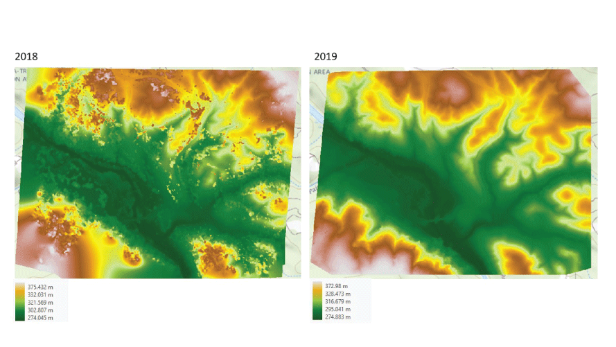
Elevation at Paige Bar NEED Camp from unoccupied aircraft system surveys in fall 2018 (digital surface model) and spring 2019 (digital elevation model).

Example of unoccupied aircraft system datasets (spring 2019) from the Paige Bar NEED Camp in Whiskeytown National Recreation Area. A, The digital elevation model (DEM) was created from a Ricoh sensor with a resolution of 3.4 centimeters (cm); B, the normalized difference vegetation index (NDVI) image was created from the MicaSense sensor with a resolution of 8 cm. NDVI is a measure of greenness with high values identifying green healthy vegetation. NDVI values from 0.00 to 0.02 are scaled to 0–200; and C, the Infrared image is a false-color composite (MicaSense). All site maps are in appendix 1.
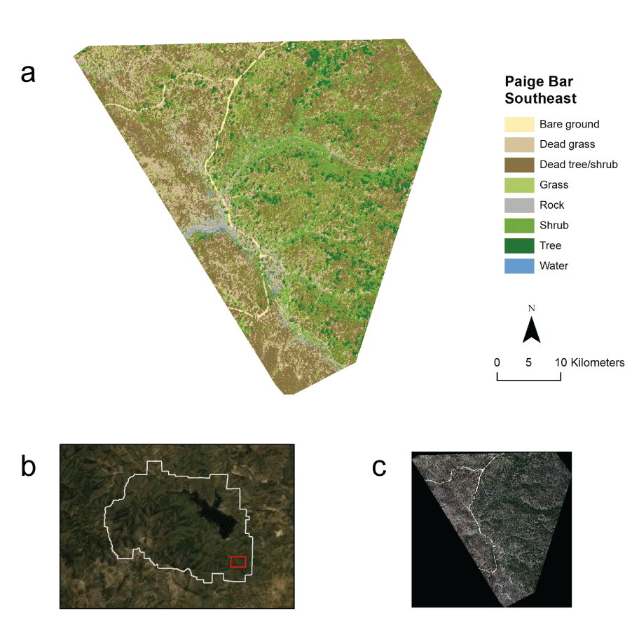
In 2018, a total of 119 flights were conducted (approximately 23 hours of flight time), and in 2019, 142 flights were conducted (approximately 25 hours of flight time) for vegetation surveys using the MicaSense sensor. Land-cover classification based on the random forest model produced high-resolution maps of ground cover at seven sites (fig. 17; appendix 1). The predictive accuracy of the random forest models ranged from 0.05 to 0.53 percent across all seven sites. The most important variables in land cover classification varied greatly by site. Across all sites, the most important spectral variables were the green band, red edge band, NDVI, and MSAVI. The digital elevation and digital surface models were equally important in classification (table 3). As predicted, dead vegetation cover was higher than live vegetation across classified sites (60–85 percent versus 11–33 percent) at 8 months post-fire. Among live vegetation, shrub cover was the highest at each site (8–24 percent) followed by tree (1–10 percent) and grass (1–4 percent) cover. Canopy height loss was measured at six sites, those with high-resolution surface models (DSMs) from 2018 and 2019 (table 2). The canopy vegetation loss maps identified areas with delayed post-fire biomass loss through fallen leaves, stems, and trunks (fig. 18). Combined with post-fire debris flow hazard probabilities (U.S. Geological Survey, 2022), it may be possible to identify high-risk areas (that is, areas with high probability of debris flow and post-fire debris accumulation; fig. 18; appendix 1).
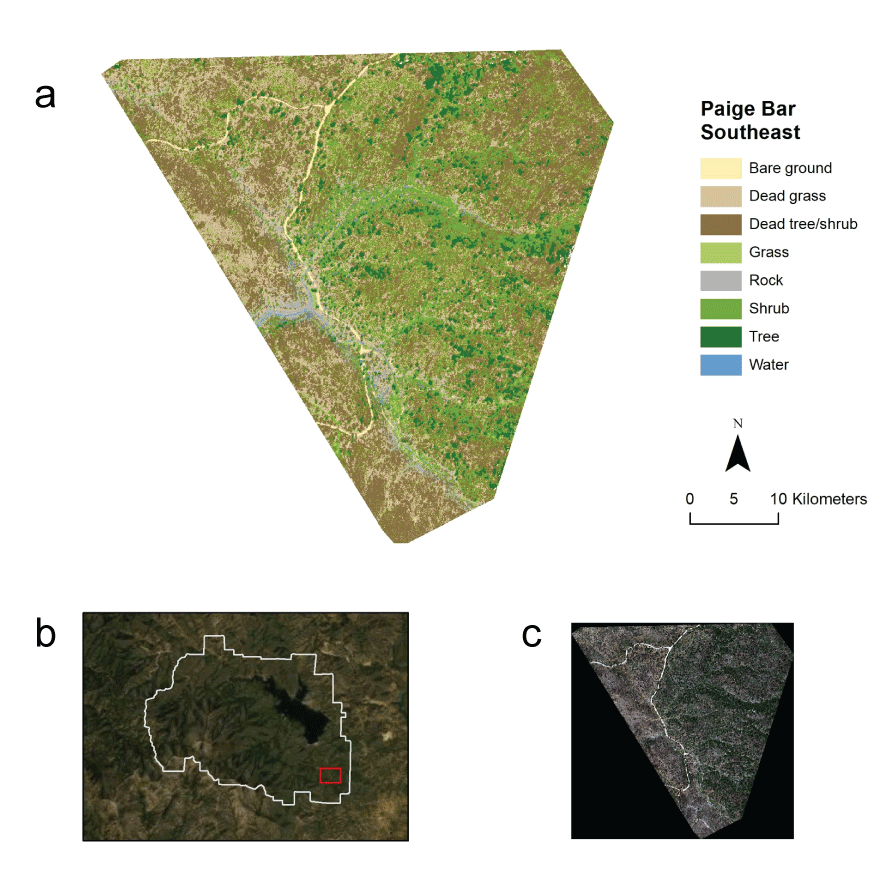
A, Land cover classification from a random forest model at the Paige Bar Southeast site; B, with site location relative to Whiskeytown National Recreation Area boundary; and C, true color image. All site classifications are in appendix 1.
Table 3.
Random forest model accuracy and variable importance by site.[%, percent; DEM, digital elevation model; NDVI, normalized difference vegetation index; DSM, digital surface model; MSAVI, modified soil adjusted vegetation index]
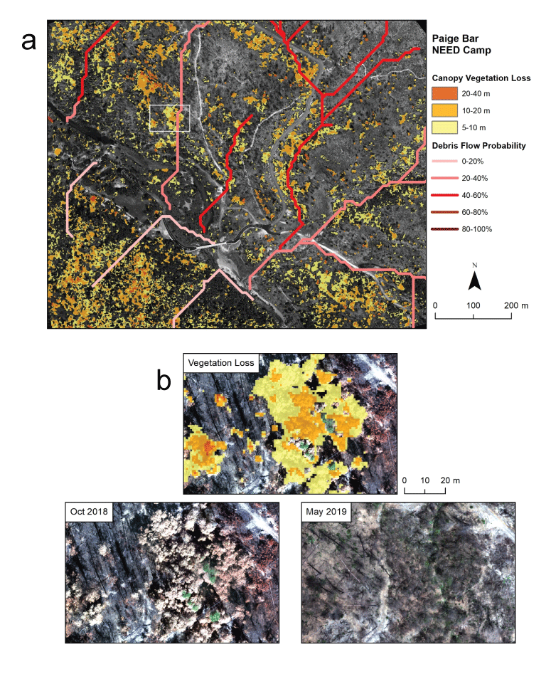
A, Debris flow risk maps with canopy vegetation loss and post-fire debris flow hazard assessment at the Paige Bar NEED camp; and B, with close-up example of vegetation loss between 2018 and 2019. All site risk maps are in appendix 1.
Summary
Our plot-based field data generally confirmed remotely sensed assessments of fire severity, finding steep declines in average live tree basal area and stem density with increasing fire severity categories. Losses were especially apparent in small trees (for example, less than 15-centimeters diameter at breast height), which are typically missed in remotely sensed surveys. Greater loss of small trees is not surprising because protective features such as thick bark and high tree crowns scale positively with tree size (Hood and others, 2018). We detected generally similar patterns in post-fire mortality across major tree genera. Although tree species have variable vulnerability to fire (Stevens and others, 2020), high-intensity fires such as the Carr Fire have the potential to overwhelm even large, fire-resistant trees. We detected an exception to these patterns with hardwood genera, such as Notholithocarpus and Quercus, where small tree stem density was high likely due to post-fire resprouting. This finding highlights the difference in post-fire response between sprouting and non-sprouting genera, where sprouting species may dominate in the years immediately after fire (Pausas and Keeley, 2014). If additional major fires do not occur in the period required for regenerating conifers to establish and grow to fire-resistant sizes (approximately 50–100 years), forests may recover to conditions resembling forests before the Carr Fire. If another major wildfire were to occur in the next few decades, it has the potential to set the stage for a more permanent vegetation type conversion, with landscapes dominated by resprouting shrubs, hardwood species, and nonnative grasses (Falk and others, 2022). Additional years of observation are needed to fully gauge the recovery trajectory of these forests after the Carr Fire.
Old growth forests at Whiskeytown National Recreation Area (WHIS) appeared to be heavily affected by the Carr Fire. At WHIS, old growth forests contain large trees that serve as biological legacies (Parsons and DeBenedetti, 1979) and include a large fraction of biomass within forests (Lutz and others, 2012). There are many reports that large trees are declining in the western United States and elsewhere (Lutz and others, 2009). Even in the absence of high-severity fire, large trees may be declining because of other stressors, such as drought and pest activity (reviewed in Lutz and others, 2009; Lindenmayer and others, 201413). The loss of large trees in U.S. national parks is concerning because these areas were often created to conserve landscapes and features that were present at the time of park establishment. The temporal scale at which large trees will again be common in the severely burned areas of WHIS will likely be on the order of centuries.
There was high potential of erosion after the Carr Fire because it occurred in late summer, was fully contained by August 2018, and preceded a relatively wet winter. However, we were unable to calculate differences in unoccupied aircraft system-derived digital elevation models from fall 2018 and spring 2019 because of highly variable ground elevation values from differing flight patterns. We did detect canopy vegetation loss between 2018 and 2019. This loss could be used to track potential debris accumulation resulting in increased flow risk, particularly in areas with modeled high probabilities of debris flow (U.S. Geological Survey, 2022). In addition to canopy vegetation loss, dead vegetation was more widespread than live vegetation 8 months post-fire. Tracking vegetation cover and new loss is important for post-fire monitoring and management because the risk of debris flow remains elevated for 2 to10 years after a wildfire (Cannon and others, 2010; DeGraff and others, 2015).
How these forests at WHIS develop after the Carr Fire is contingent on unknown future conditions, such as the probability of additional disturbances like high-severity fire and drought (which may cause additional tree mortality and impede the establishment and growth of conifers). Managers at WHIS may wish to prioritize actions that minimize the likelihood of occurrence or reduce the severity of future disturbances. The use of fuel treatments, such as mechanical thinning and prescribed fire, may reduce future fire severity and allow greater flexibility in the management of future fires. Mechanical thinning operations, where appropriate, may also reduce the moisture stress of residual trees (Sankey and Tatum, 2022). Fuel and stand structure management may help increase the resilience of these forests to future disturbance and reduce the potential for vegetation type conversions (Falk and others, 2022).
References Cited
Agisoft LLC, 2021, Agisoft Metashape 1.6.5—Professional edition: St. Petersburg, Russia, Agisoft LLC software, accessed June 22, 2023, at https://www.agisoft.com/downloads/installer/.
Cannon, S.H., Gartner, J.E., Rupert, M.G., Michael, J.A., Rea, A.H., and Parrett, C., 2010, Predicting the probability and volume of post-wildfire debris flows in the intermountain western United States: Geological Society of America Bulletin, v. 122, no. 1–2, p. 127–144. [Available at https://doi.org/10.1130/B26459.1.]
DeGraff, J.V., Cannon, S.H., and Gartner, J.E., 2015, The timing of susceptibility to post-fire debris flows in the western United States: Environmental & Engineering GeoScience, v. 21, no. 4, p. 277–292. [Available at https://doi.org/10.2113/gseegeosci.21.4.277.]
Falk, D.A., van Mantgem, P.J., Keeley, J.E., Gregg, R.M., Guiterman, C.H., Tepley, A.J., Young, D.J.N., and Marshall, L.A., 2022, Mechanisms of forest resilience: Forest Ecology and Management, v. 512, article 120129. [Available at https://doi.org/10.1016/j.foreco.2022.120129.]
Folke, C., Carpenter, S., Walker, B., Scheffer, M., Elmqvist, T., Gunderson, L., and Holling, C.S., 2004, Regime shifts, resilience, and biodiversity in ecosystem management: Annual Review of Ecology, Evolution, and Systematics, v. 35, no. 1, p. 557–581. [Available at https://doi.org/10.1146/annurev.ecolsys.35.021103.105711.]
Fonstad, M.A., Dietrich, J.T., Courville, B.C., Jensen, J.L., and Carbonneau, P.E., 2013, Topographic structure from motion—A new development in photogrammetric measurement: Earth Surface Processes and Landforms, v. 38, no. 4, p. 421–430. [Available at https://doi.org/10.1002/esp.3366.]
Fry, D.L., and Stephens, S.L., 2006, Influence of humans and climate on the fire history of a ponderosa pine-mixed conifer forest in the southeastern Klamath Mountains, California: Forest Ecology and Management, v. 223, nos. 1–3, p. 428–438. [Available at https://doi.org/10.1016/j.foreco.2005.12.021.]
Hagmann, R.K., Hessburg, P.F., Prichard, S.J., Povak, N.A., Brown, P.M., Fulé, P.Z., Keane, R.E., Knapp, E.E., Lydersen, J.M., Metlen, K.L., Reilly, M.J., Sánchez Meador, A.J., Stephens, S.L., Stevens, J.T., Taylor, A.H., Yocom, L.L., Battaglia, M.A., Churchill, D.J., Daniels, L.D., Falk, D.A., Henson, P., Johnston, J.D., Krawchuk, M.A., Levine, C.R., Meigs, G.W., Merschel, A.G., North, M.P., Safford, H.D., Swetnam, T.W., and Waltz, A.E.M., 2021, Evidence for widespread changes in the structure, composition, and fire regimes of western North American forests: Ecological Applications, v. 31, no. 8, article e02431. [Available at https://doi.org/10.1002/eap.2431.]
Holling, C.S., 1973, Resilience and stability of ecological systems: Annual Review of Ecology and Systematics, v. 4, no. 1, p. 1–23. [Available at https://doi.org/10.1146/annurev.es.04.110173.000245.]
Hood, S.M., Varner, J.M., van Mantgem, P., and Cansler, C.A., 2018, Fire and tree death—Understanding and improving modeling of fire-induced tree mortality: Environmental Research Letters, v. 13, no. 11, article 113004. [Available at https://doi.org/10.1088/1748-9326/aae934.]
Lareau, N.P., Nauslar, N.J. and Abatzoglou, J.T., 2018, The Carr Fire vortex—A case of pyrotornadogenesis?: Geophysical Research Letters, v. 45, no. 23, p. 13107–13115. [Available at https://doi.org/10.1029/2018GL080667.]
Leonzo, C.M., and Keyes, C.R., 2010, Fire-excluded relict forests in the southeastern Klamath Mountains, California, USA: Fire Ecology, v. 6, no. 3, p. 62–76. [Available at https://doi.org/10.4996/fireecology.0603062.]
Lindenmayer, D.B., Laurance, W.F., Franklin, J.F., Likens, G.E., Banks, S.C., Blanchard, W., Gibbons, P., Ikin, K., Blair, D., McBurney, L., Manning, A.D., and Stein, J.A.R., 2014, New policies for old trees—Averting a global crisis in a keystone ecological structure: Conservation Letters, v. 7, no. 1, p. 61–69. [Available at https://doi.org/10.1111/conl.12013.]
Lutz, J.A., Larson, A.J., Swanson, M.E., and Freund, J.A., 2012, Ecological importance of large-diameter trees in a temperate mixed-conifer forest: PLOS One, v. 7, no. 5, article e36131. [Available at https://doi.org/10.1371/journal.pone.0036131.]
Lutz, J.A., van Wagtendonk, J.W., and Franklin, J.F., 2009, Twentieth-century decline of large-diameter trees in Yosemite National Park, California, USA: Forest Ecology and Management, v. 257, no. 11, p. 2296–2307. [Available at https://doi.org/10.1016/j.foreco.2009.03.009.]
Millar, C.I., and Stephenson, N.L., 2015, Temperate forest health in an era of emerging megadisturbance: Science, v. 349, no. 6250, p. 823–826. [Available at https://doi.org/10.1126/science.aaa9933.]
National Park Service, 2003, Fire monitoring handbook: Boise, Idaho, Fire Management Program Center, National Interagency Fire Center, 274 p. [Available at https://www.nps.gov/orgs/1965/upload/fire-effects-monitoring-handbook.pdf.]
Odion, D.C., Sarr, D.A., Mohren, S.R., and Smith, S.B., 2011, Monitoring vegetation composition, structure, and function in the parks of the Klamath Network: Natural Resource Report NPS/KLMN/NRR-2011/401, National Park Service, Fort Collins, Colo., 243 p. [Available at https://www.researchgate.net/publication/278668448_Monitoring_Vegetation_Composition_Structure_and_Function_in_the_Parks_of_the_Klamath_Network.]
Parsons, D.J., and DeBenedetti, S.H., 1979, Impact of fire suppression on a mixed-conifer forest: Forest Ecology and Management, v. 2, p. 21–33. [Available at https://doi.org/10.1016/0378-1127(79)90034-3.]
Pausas, J.G., and Keeley, J.E., 2014, Evolutionary ecology of resprouting and seeding in fire-prone ecosystems: New Phytologist, v. 204, no. 1, p. 55–65. [Available at https://doi.org/10.1111/nph.12921.]
Petraitis, P., 2013, Multiple stable states in natural ecosystems: Oxford, England, Oxford University Press, 188 p. [Available at https://doi.org/10.1093/acprof:osobl/9780199569342.001.0001.]
Sankey, T., and Tatum, J., 2022, Thinning increases forest resiliency during unprecedented drought: Scientific Reports, v. 12, article 9041. [Available at https://doi.org/10.1038/s41598-022-12982-z.]
Scott, J.H., and Burgan, R.E., 2005, Standard fire behavior fuel models—A comprehensive set for use with Rothermel’s surface fire spread model: Ft. Collins, Colo., U.S. Department of Agriculture, Forest Service, Rocky Mountain Research Station, General Technical Report RMRS-GTR-153, 72 p. [Available at https://doi.org/10.2737/RMRS-GTR-153.]
Skinner, C.N., 1995, Change in spatial characteristics of forest openings in the Klamath Mountains of northwestern California, USA: Landscape Ecology, v. 10, no. 4, p. 219–228. [Available at https://doi.org/10.1007/BF00129256.]
Smith, S.B., van Mantgem, P.J., and Odion, D., 2021, Vegetation community monitoring—Species composition and biophysical gradients in Klamath Network parks: Ft. Collins, Colo., National Park Service, Natural Resource Report NPS/KLMN/NRR-2021/2236. [Available at https://doi.org/10.36967/nrr-2284769.]
Stephens, S.L., and Ruth, L.W., 2005, Federal forest-fire policy in the United States: Ecological Applications, v. 15, no. 2, p. 532–542. [Available at https://doi.org/10.1890/04-0545.]
Stevens, J.T., Kling, M.M., Schwilk, D.W., Varner, J.M., and Kane, J.M., 2020, Biogeography of fire regimes in western U.S. conifer forests—A trait‐based approach: Global Ecology and Biogeography, p. 944–955. [Available at https://doi.org/10.1111/geb.13079.]
Stewart, J.A.E., van Mantgem, P.J., Young, D.J.N., Shive, K.L., Preisler, H.K., Das, A.J., Stephenson, N.L., Keeley, J.E., Safford, H.D., Wright, M.C., Welch, K.R., and Thorne, J.H., 2021, Effects of postfire climate and seed availability on postfire conifer regeneration: Ecological Applications, v. 31, no. 3, article e02280. [Available at https://doi.org/10.1002/eap.2280.]
Taylor, A.H., 2000, Fire regimes and forest changes in mid and upper montane forests of the southern Cascades, Lassen Volcanic National Park, California, U.S.A.: Journal of Biogeography, v. 27, no. 1, p. 87–104. [Available at https://doi.org/10.1046/j.1365-2699.2000.00353.x.]
Thorne, K.M., Freeman, C.M., Colley, A., and Rankin, L.L., 2024, UAS imagery at Whiskeytown National Recreation Area in 2018 and 2019 following the Carr Fire: U.S. Geological Survey data release, available at https://doi.org/10.5066/P9GS9V1J.
Ullman, S., 1979, The interpretation of structure from motion: Proceedings of the Royal Society B, Biological Sciences, v. 203, no. 1153, p. 405–426. [Available at https://doi.org/10.1098/rspb.1979.0006.]
U.S. Department of the Interior, 2003, Whiskeytown fire management plan and draft environmental impact statement: Pacific West Region, Whiskeytown National Recreation Area, U.S. Department of the Interior, National Park Service, 329 p. [Available at https://pubs.nps.gov/eTIC/WEPO-WI/WHIS_611_03017_0346pg.pdf.]
U.S. Geological Survey, 2022, Emergency assessment of post-fire debris-flow hazards: U.S. Geological Survey, accessed September 7, 2022, at https://landslides.usgs.gov/hazards/postfire_debrisflow.
Westoby, M.J., Brasington, J., Glasser, N.F., Hambrey, M.J., and Reynolds, J.M., 2012, ‘Structure-from-motion’ photogrammetry—A low-cost, effective tool for geoscience applications: Geomorphology, v. 179, p. 300–314. [Available at https://doi.org/10.1016/j.geomorph.2012.08.021.]
Wright, M.C., Engber, E., and van Mantgem, P.J., 2024, Forest conditions following the 2018 Carr Fire at Whiskeytown National Recreation Area: U.S. Geological Survey data release, available at https://doi.org/10.5066/P97Y21L1.
Wright, M.C., Stewart, J.A.E., van Mantgem, P.J., Young, D.J.N., Shive, K.L., Preisler, H.K., Das, A.J., Stephenson, N.L., Keeley, J.E., Safford, H.D., Welch, K.R., and Thorne, J.H., 2020, poscrptR (version 0.1.3): U.S. Geological Survey software release, available at https://code.usgs.gov/werc/redwood_field_station/poscrptr.
Glossary
- basal area
Summed cross-sectional area of live tree stems at breast height (1.37 meters) per unit area.
- DBH
Tree stem diameter at breast height (1.37 meters).
- LANDSAT
A space-based remotely sensed imagery of the Earth’s surface, active since the mid-1970s.
- MTBS
A remotely sensed assessment of burn severity and fire perimeters. Assessments are based on pre-fire and 1-year post-fire conditions from LANDSAT imagery.
- RAVG
A remotely sensed assessment of burn severity and fire perimeters. Assessments are based on pre-fire and immediate post-fire (30–45 days post-fire) conditions from LANDSAT imagery.
- stem density
Count of live tree stems per unit area.
Appendix 1. Unoccupied Aircraft System Imagery
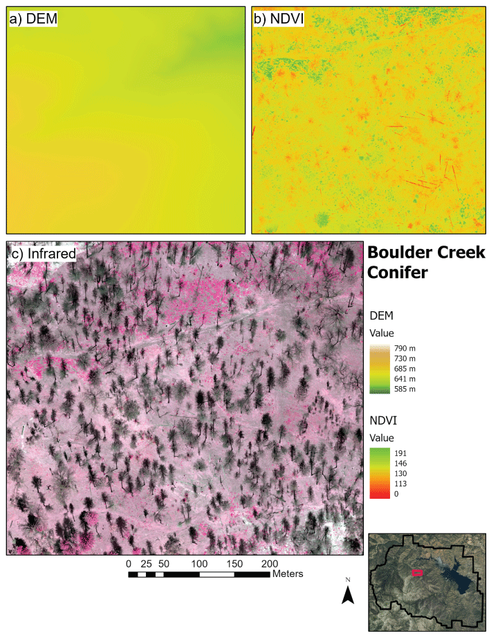
Unoccupied aircraft system products for Boulder Creek Conifer site at Whiskeytown National Recreation Area. A, 2018 digital elevation model (DEM); B, normalized difference vegetation index (NDVI); and C, false color infrared orthomosaic image.
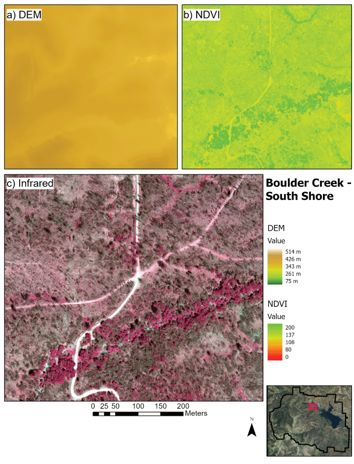
A, Digital elevation model (DEM); B, normalized difference vegetation index (NDVI); and C, a false color infrared image at the Boulder Creek South Shore site.
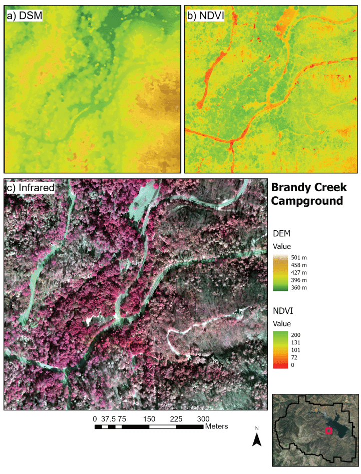
A, Digital surface model (DSM); B, normalized difference vegetation index (NDVI); and C, a false color infrared image at the Brandy Creek Campground site.
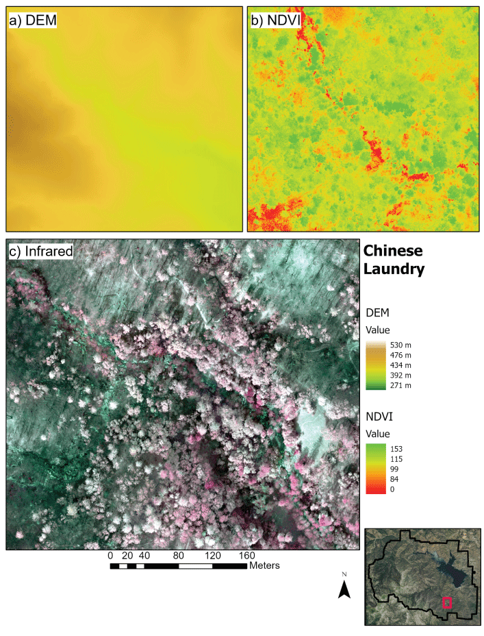
A, Digital elevation model (DEM); B, normalized difference vegetation index (NDVI), and C, a false color infrared image at the Chinese Laundry site.
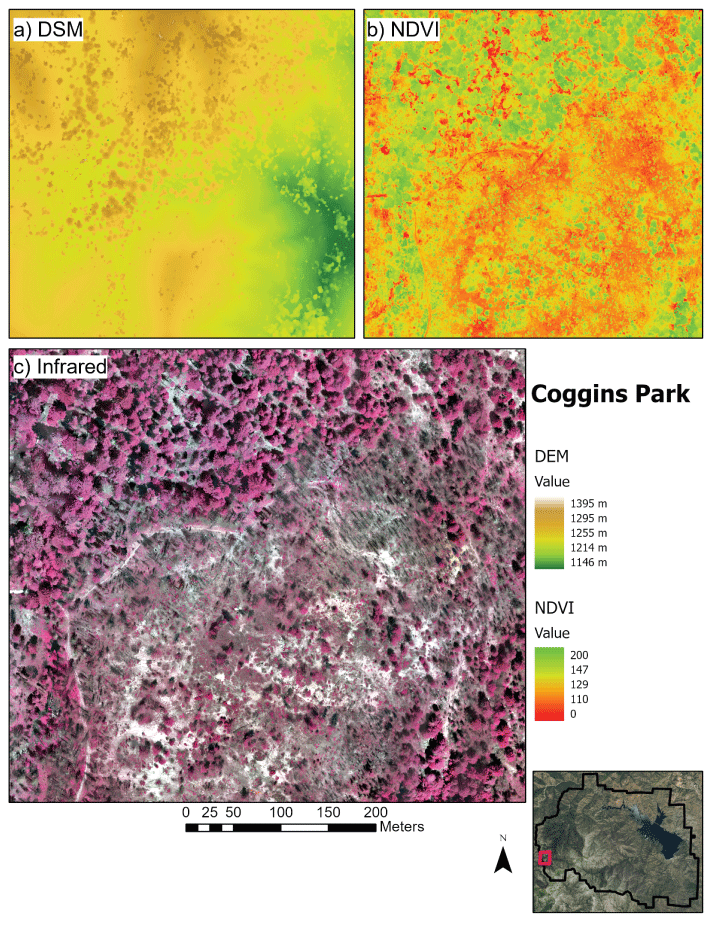
A, Digital surface model (DSM); B, normalized difference vegetation index (NDVI); and C, a false color infrared image at the Coggins Park site.
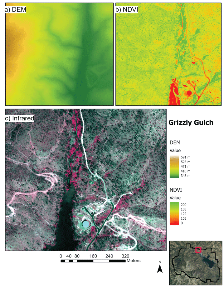
A, Digital elevation model (DEM); B, normalized difference vegetation index (NDVI); and C, a false color infrared image at the Grizzly Gulch site.
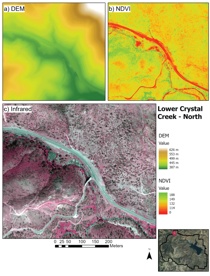
A, Digital elevation model (DEM); B, normalized difference vegetation index (NDVI); and C, a false color infrared image at the Lower Crystal Creek North site.
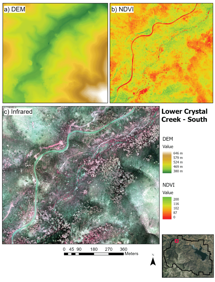
A, Digital elevation model (DEM); B, normalized difference vegetation index (NDVI); and C, a false color infrared image at the Lower Crystal Creek South site.
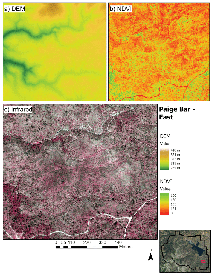
A, Digital elevation model (DEM); B, normalized difference vegetation index (NDVI); and C, a false color infrared image at the Paige Bar East site.
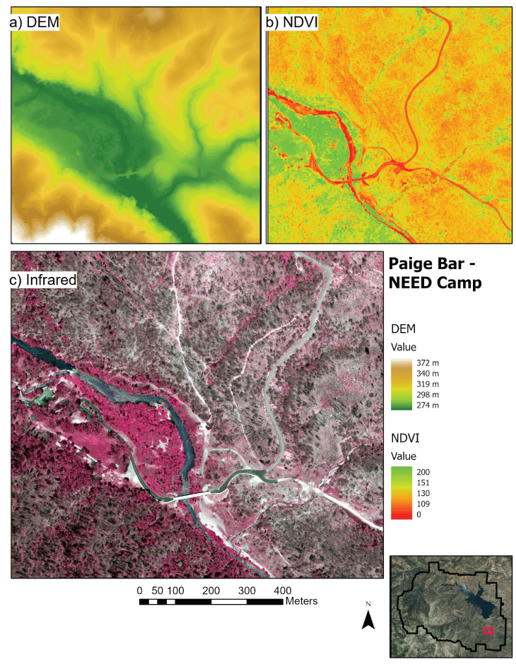
A, Digital elevation model (DEM); B, normalized difference vegetation index (NDVI); and C, a false color infrared image at the Paige Bar NEED Camp.
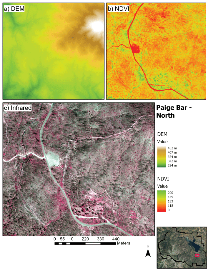
A, Digital elevation model (DEM); B, normalized difference vegetation index (NDVI); and C, a false color infrared image at the Paige Bar North site.
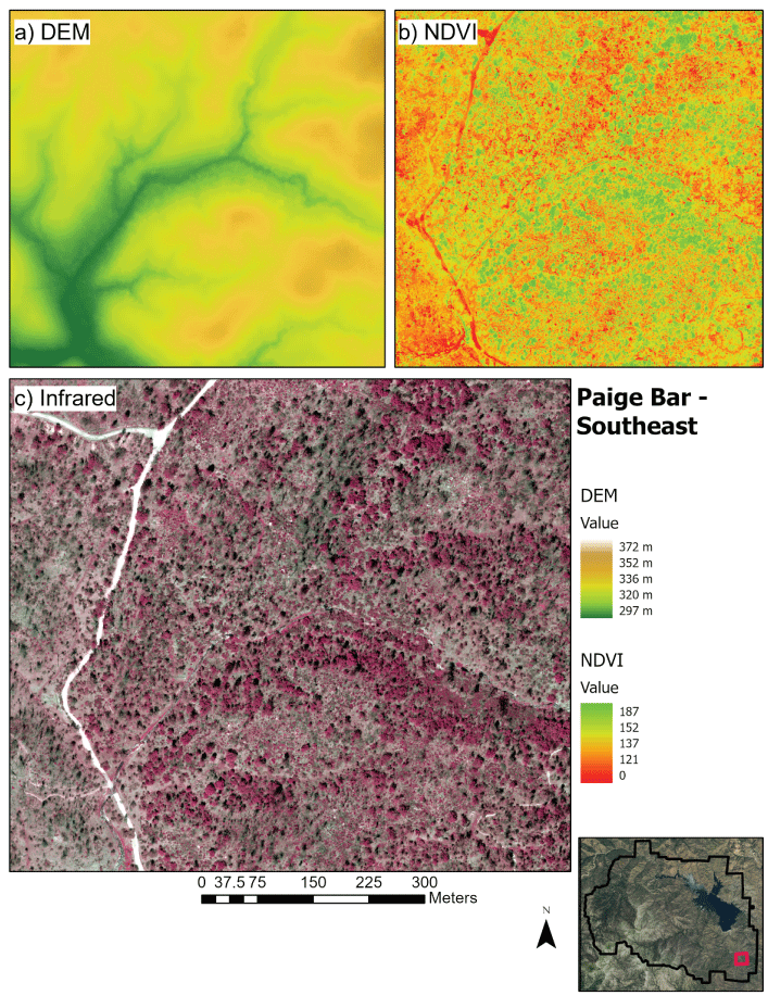
A, Digital elevation model (DEM); B, normalized difference vegetation index (NDVI); and C, a false color infrared image at the Paige Bar Southeast site.
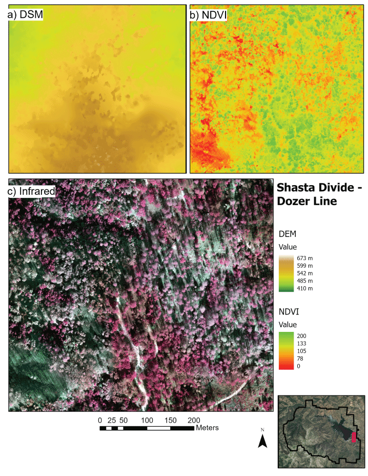
A, Digital surface model (DSM); B, normalized difference vegetation index (NDVI); and C, a false color infrared image at the Shasta Divide Dozer Line site.
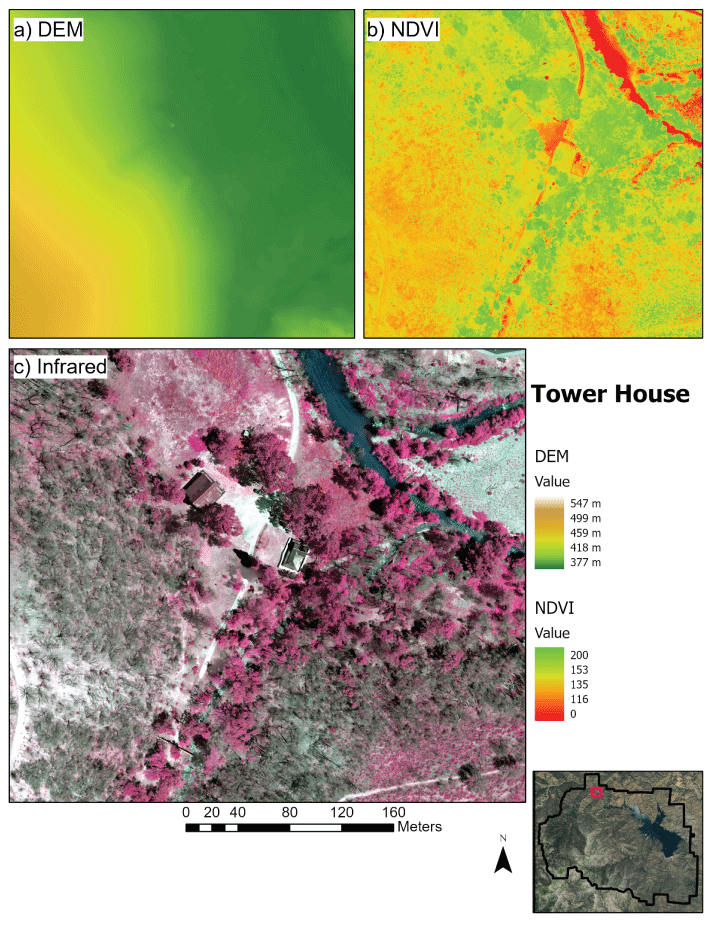
A, Digital elevation model (DEM); B, normalized difference vegetation index (NDVI); and C, a false color infrared image at the Tower House site.
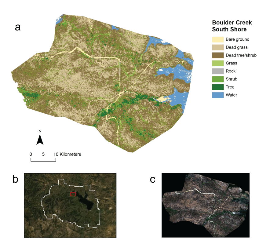
A, Land cover classification from a random forest model at the Boulder Creek South Shore site; B, with site location relative to the Whiskeytown National Recreation Area boundary; and C, true color image.
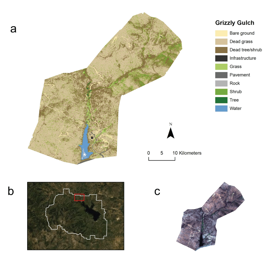
A, Land cover classification from a random forest model at the Grizzly Gulch site; B, with site location relative to the Whiskeytown National Recreation Area boundary; and C, true color image.
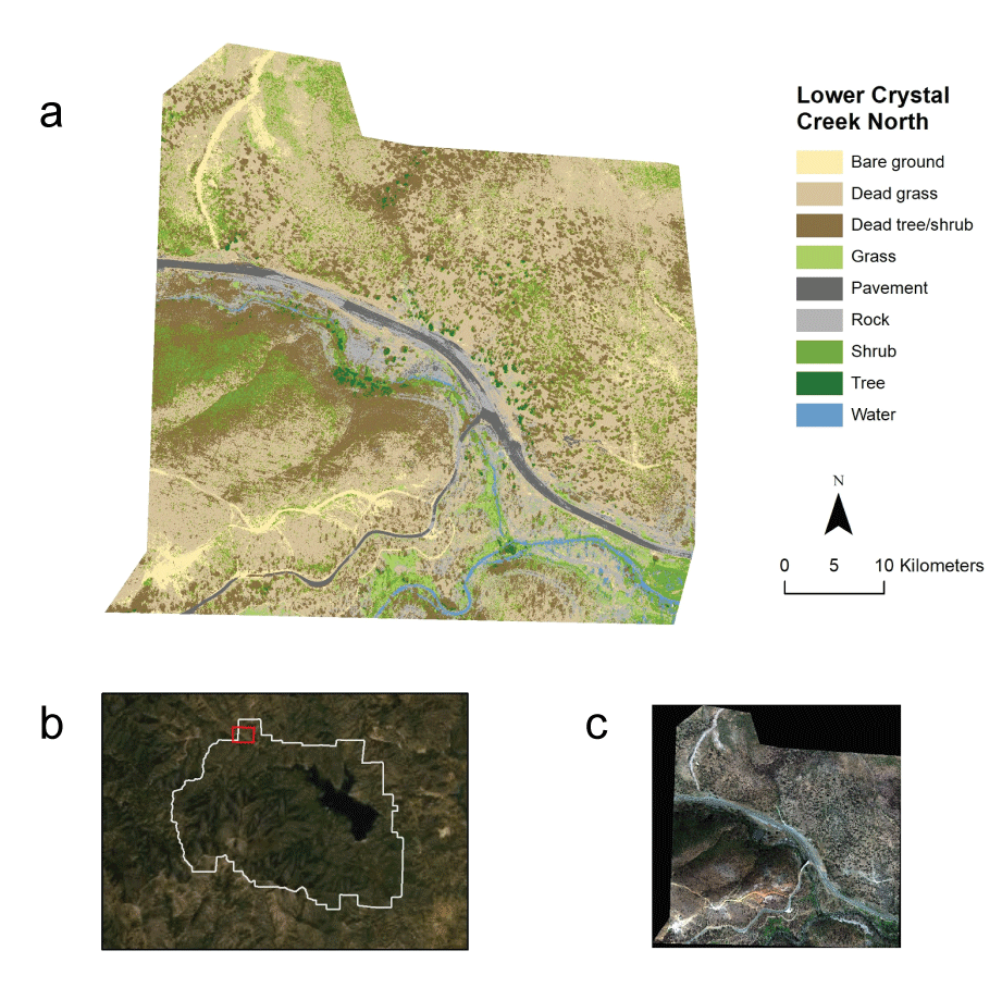
A, Land cover classification from a random forest model at the Lower Crystal Creek North site; B, with site location relative to WHIS boundary; and C, true color image.
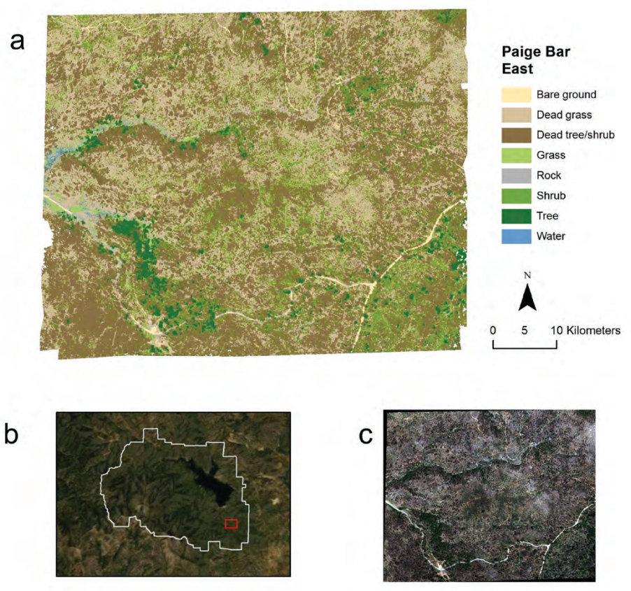
A, Land cover classification from a random forest model at the Paige Bar East site; B, with site location relative to the Whiskeytown National Recreation Area boundary; and C, true color image.
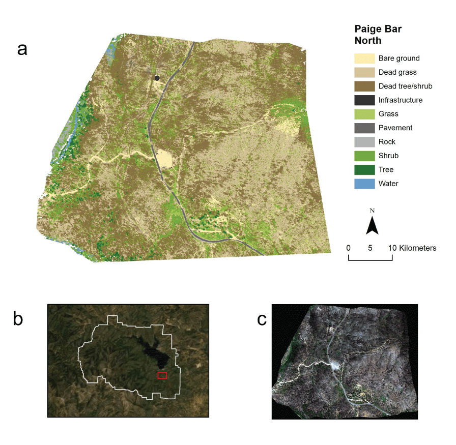
A, Land cover classification from a random forest model at the Paige Bar North site; B, with site location relative to the Whiskeytown National Recreation Area boundary; and C, true color image.
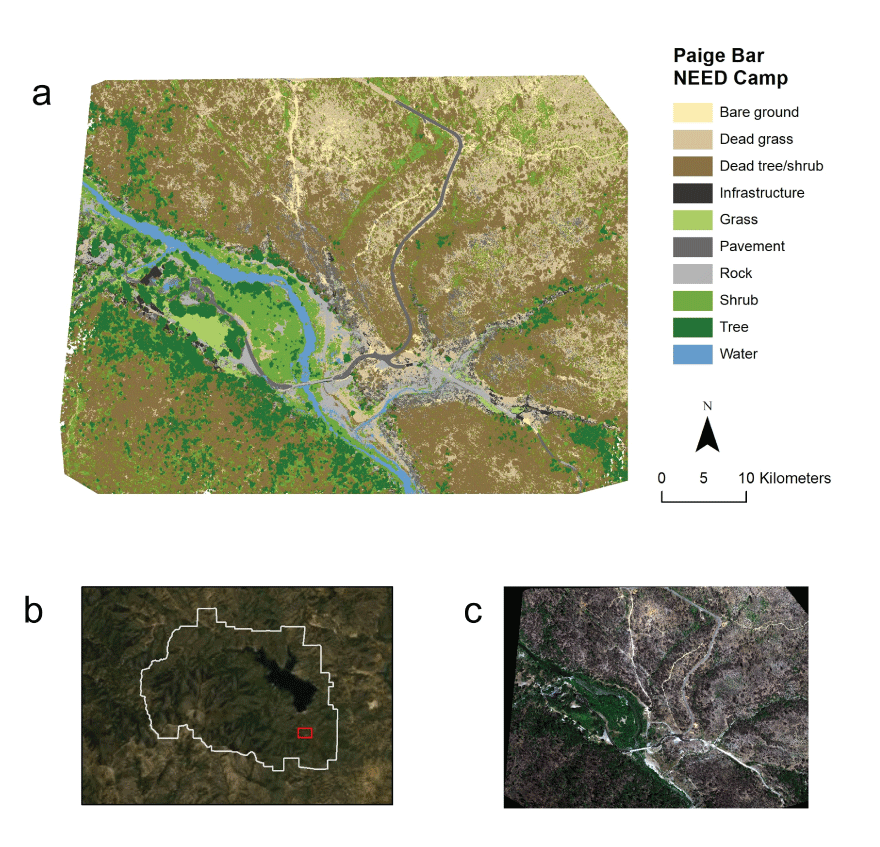
A, Land cover classification from a random forest model at the Paige Bar NEED Camp; B, with site location relative to the Whiskeytown National Recreation Area boundary; and C, true color image.
A, Land cover classification from a random forest model at the Paige Bar Southeast site; B, with site location relative to the Whiskeytown National Recreation Area boundary; and C, true color image.
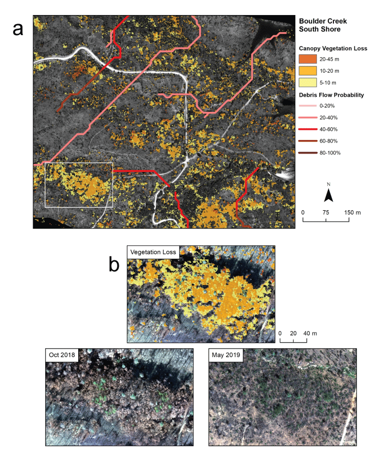
A, Debris flow risk maps with canopy vegetation loss and post-wildfire debris flow hazard assessment at the Boulder Creek South Shore site; and B, with close-up example of vegetation loss between 2018 and 2019.
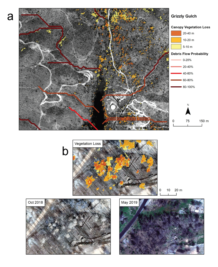
A, Debris flow risk maps with canopy vegetation loss and post-wildfire debris flow hazard assessment at the Grizzly Gulch site; and B, with close-up example of vegetation loss between 2018 and 2019.
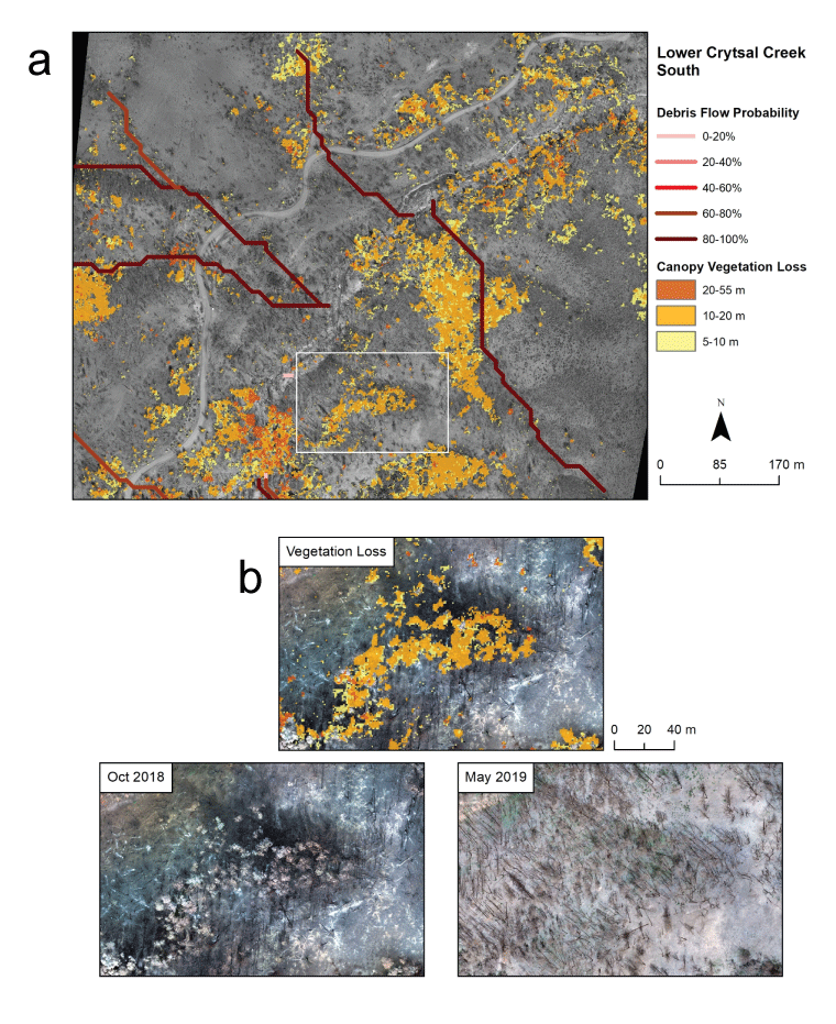
A, Debris flow risk maps with canopy vegetation loss and post-wildfire debris flow hazard assessment at the Lower Crystal Creek South site; and B, with close-up example of vegetation loss between 2018 and 2019.
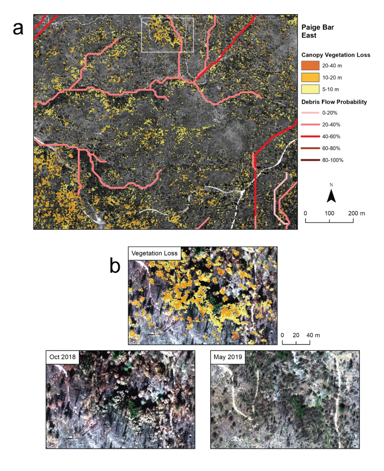
A, Debris flow risk maps with canopy vegetation loss and post-wildfire debris flow hazard assessment at the Paige Bar East site; and B, with close-up example of vegetation loss between 2018 and 2019.
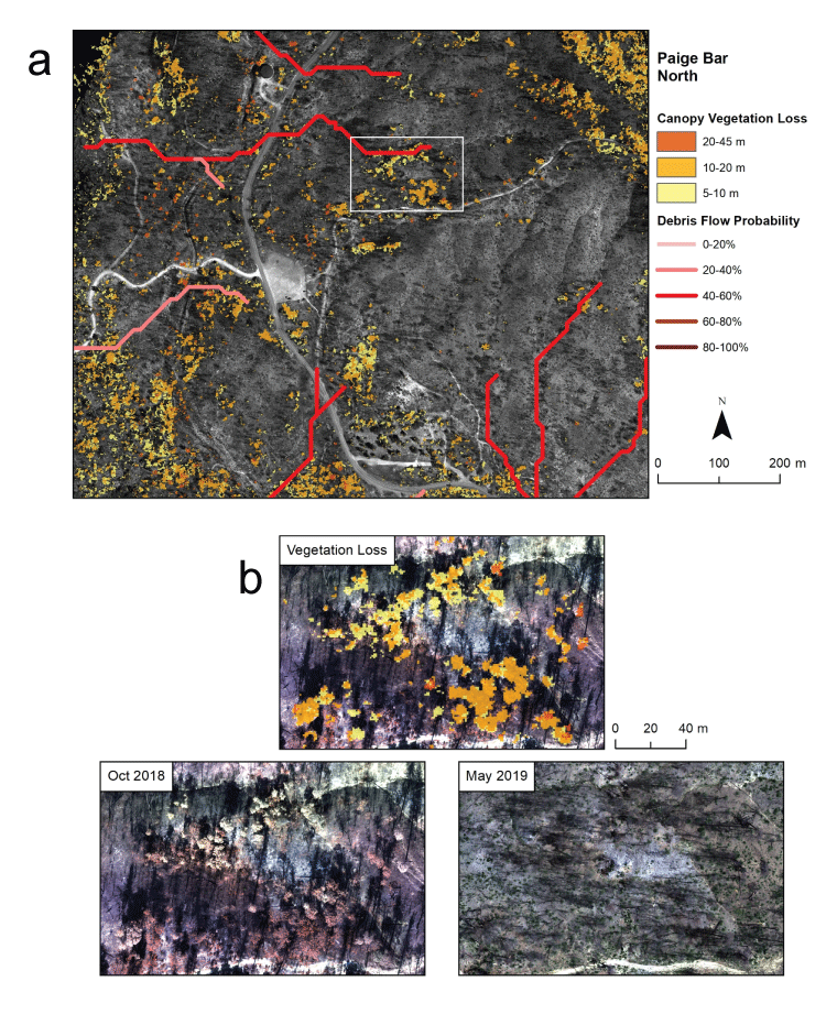
A, Debris flow risk maps with canopy vegetation loss and post-wildfire debris flow hazard assessment at the Paige Bar North site; and B, with close-up example of vegetation loss between 2018 and 2019.
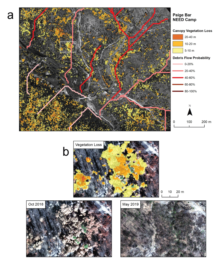
A, Debris flow risk maps with canopy vegetation loss and post-wildfire debris flow hazard assessment at the Paige Bar NEED Camp; and B, with close-up example of vegetation loss between 2018 and 2019.
Conversion Factors
Temperature in degrees Celsius (°C) may be converted to degrees Fahrenheit (°F) as follows:
°F = (1.8 × °C) + 32.
Temperature in degrees Fahrenheit (°F) may be converted to degrees Celsius (°C) as follows:
°C = (°F − 32) / 1.8.
Abbreviations
AGL
above ground level
DBH
diameter at breast height
DEM
digital elevation model
DSM
digital surface model
FMH
Fire Monitoring Handbook
GPS
Global Positioning System
I&M
Inventory and Monitoring
Lidar
Light Detection and Ranging
MTBS
Monitoring Trends in Burn Severity
NDVI
Normalized Difference Vegetation Index
NPS
National Park Service
UAS
unoccupied aircraft system
WHIS
Whiskeytown National Recreation Area
For more information concerning the research in this report, contact the
Director, Western Ecological Research Center
U.S. Geological Survey
3020 State University Drive East
Sacramento, California 95819
https://www.usgs.gov/centers/werc
Publishing support provided by the U.S. Geological Survey Science Publishing Network, Sacramento Publishing Service Center
Disclaimers
Any use of trade, firm, or product names is for descriptive purposes only and does not imply endorsement by the U.S. Government.
Although this information product, for the most part, is in the public domain, it also may contain copyrighted materials as noted in the text. Permission to reproduce copyrighted items must be secured from the copyright owner.
Suggested Citation
van Mantgem, P.J., Wright, M.C., Thorne, K.M., Beckmann, J., Buffington, K., Rankin, L.L., Colley, A., and Engber, E.A., 2024, Learning from a high-severity fire event—Conditions following the 2018 Carr Fire at Whiskeytown National Recreation Area: U.S. Geological Survey Open-File Report 2023–1053, 52 p., https://doi.org/10.3133/ofr20231053.
ISSN: 2331-1258 (online)
Study Area
| Publication type | Report |
|---|---|
| Publication Subtype | USGS Numbered Series |
| Title | Learning from a high-severity fire event—Conditions following the 2018 Carr Fire at Whiskeytown National Recreation Area |
| Series title | Open-File Report |
| Series number | 2023-1053 |
| DOI | 10.3133/ofr20231053 |
| Publication Date | August 30, 2024 |
| Year Published | 2024 |
| Language | English |
| Publisher | U.S. Geological Survey |
| Publisher location | Reston, VA |
| Contributing office(s) | Western Ecological Research Center |
| Description | Report: viii, 52 p.; 2 Data Releases |
| Country | United States |
| State | California |
| Other Geospatial | Whiskeytown National Recreation Area |
| Online Only (Y/N) | Y |