

Application of the Stream Salmonid Simulator (S3) Model to Assess Fall Chinook Salmon (Oncorhynchus tshawytscha) Production in the American River, California
Links
- Document: Report (5.6 MB pdf) , HTML , XML
- Download citation as: RIS | Dublin Core
Acknowledgments
We are grateful to the many entities, agencies, and field staff that have collected and provided data to inform the Stream Salmonid Simulator for the American River. From our colleagues at the U.S. Geological Survey, we extend our gratitude to Phil Haner, Brad Liedtke, Ryan Tomka, Jill Hardiman, and Joe Warren for their diligence in data collection whether rain or shine. From outside the U.S. Geological Survey, we’d like to thank Logan Day (Pacific States Marine Fisheries Commission) for providing the abundance estimates of juvenile fall Chinook salmon (Oncorhynchus tshawytscha) passing the fish trap required to fit the Stream Salmonid Simulator (S3) model parameters, and Tracy Grimes (California Department of Fish and Wildlife) for providing spawning escapement estimates that are foundational and integral to all S3 simulations. This modeling would not be possible without all their contributions.
Executive Summary
Anadromous fish returning to the lower American River are restricted to 36 kilometers of free-flowing river between Nimbus Dam and American River’s confluence with the Sacramento River, California. Salmon in the American River provide an important freshwater recreational fishery. However, annual salmon production in the American River in recent years has been low relative to the mid-1990s (Surface Water Resources, Inc., 2001). To investigate the low production of fall-run Chinook salmon (Oncorhynchus tshawytscha), the Bureau of Reclamation requested that the U.S. Geological Survey apply the Stream Salmonid Simulator (S3) model to the population of fall-run Chinook salmon on the American River.
The American River was chosen among seven candidate Sacramento Basin rivers for S3 application. The American River was selected because of its management and public interest, recently low anadromous fish production, and rich time series of key demographic data needed for S3 application. Data that were not available, however, were empirical estimates on juvenile salmon habitat suitability in the American River. Therefore, a large component of applying S3 to the American River was devoted to the estimation of juvenile salmon habitat suitability and capacity. This entailed snorkeling the lower American River for 3 weeks in March 2021 during the early out-migration period for juvenile Chinook salmon. These efforts were fruitful and showed that the typically small fish (<55 millimeters) in the American River preferred much shallower depths than predicted by habitat suitability criteria derived from the literature for this population. Having empirical estimates on juvenile salmon in the American River provided a solid foundation from which to simulate the population using the S3 model.
The S3 model is a spatially explicit population model that runs on a daily time step to simulate redd superimposition, egg maturation, fry emergence and the subsequent growth, survival, and emigration of juvenile Chinook salmon from the river. The key features of this model relevant to this report include (1) a temperature-dependent bioenergetics model driving daily growth rates; (2) density-dependent dynamics that are influenced by the effect of flow on suitable habitat area; and (3) within-year habitat, river flow, and water temperature effects specific to spawning, egg incubation, and fry, parr, and smolt life stages. We used estimates of spawning escapement and geo-referenced redd locations to quantify the spatial and temporal distribution of female spawners for brood years 2014–19. These estimates of female spawners initiate the simulation of each year’s juvenile salmon emergence and emigration over a spatial domain extending from Nimbus Dam to the river’s confluence with the Sacramento River.
Using weekly estimates of juvenile salmon abundance and size (fork length) that passed the Watt Avenue fish trap (river kilometer 14.7), we calibrated the S3 model by estimating three key demographic parameters for each year, y: (1) Sy, the average daily survival probability, (2) M0y, the intercept for density-dependence in movement, representing the average daily probability of remaining in a habitat at zero abundance, and (3) Cy, the average daily proportion of maximum consumption. These parameters were obtained by minimizing the Mallow’s distance (Lupu and others, 2017) between distributions of weekly abundances and sizes of fish at the traps and weekly simulated abundances and sizes (by S3). Investigation of model fit showed excellent agreement between simulated annual abundances and the abundance of fish passing the fish trap. However, when we compared weekly abundances at the fish trap, S3 under-predicted peaks and over-predicted troughs in the time series of weekly abundances at the fish trap. Thus, some unknown within-year effects have yet to be identified and incorporated in the S3 model. Identifying these important effects and incorporating them in the S3 model would help explain the lack of fit between estimated and simulated weekly abundances.
We estimated parameters for 6 years that included a wide range of female spawner abundances (3,057–10,753) and water year types (Critical–Wet). We contrast our estimated parameters to the corresponding number of female spawners and the water year type for the Sacramento Valley. By happenstance, years having higher annual spawner abundances concurred with Critical to Dry water year types. Estimates of survival trended lower with higher spawner abundances and Critical to Dry conditions. In contrast, the extremely wet water year of 2017 had the lowest M0y, suggesting less density-dependence in fish movement, and the lowest Cy, suggesting lower average consumption in this year. When this high-flow year was excluded, a trend towards higher probabilities of fish remaining in a habitat at low abundance and lower proportions of maximum consumption was apparent from Critical to Wet conditions, but only 5 years of data were included. Except for 2017, daily proportions of maximum consumption were relatively high (Cy > 0.83), suggesting that fish were feeding at reasonably high proportions relative to the expected maximum consumption as defined by the “Wisconsin” bioenergetics model (Stewart and Ibarra, 1991).
Survival estimates from fry emergence to outmigration at the Sacramento River confluence were generally low when integrated over time. The highest daily survival probability was Sy = 0.93 in 2019, or 50 percent total mortality after 10 days. In contrast, our lowest daily survival probability was Sy = 0.74 in 2015, or 95 percent total mortality after 10 days. Consequently, even our highest estimated daily survival probability might be considered low. This is especially true given that Sy was estimated over a relatively short distance (<14.7 kilometers) from emergence to the Watt Avenue fish trap. Several factors, including our assumed and relatively high daily egg survival rate of 0.9975, could influence juvenile survival estimates. For example, an egg survival rate of 0.9975 results in 3-percent total mortality after 10 days. Egg mortality estimates used in S3 calibration were approximated from egg survivorship studies in the Yakima River, Washington (Johnson and others, 2012), and remains one of the greater uncertainties in S3 when estimating survival across life stages. By including bona fide estimates of egg survival in S3 simulations, the validity of the S3’s current daily egg survival rate could be assessed specifically for the American River. Tagging studies also could provide S3 with direct estimates of juvenile survival and movement; survival during egg incubation then could be estimated indirectly via model fitting.
Introduction
The lower American River, in northern California, is an urban watershed with a long history of development and alteration of salmon habitat. A comprehensive river corridor management plan (RCMP) was initiated for the lower American River in 2001 that included the California Resources Agency (CALFED Bay-Delta Program, 1999), the Sacramento Area Water Forum; Sacramento Area Flood Control Agency; lower American River Task Force; and Sacramento County Department of Regional Parks, Recreation, and Open Space (Surface Water Resources, Inc., 2001). The RCMP provided a planning framework for consensus building of ecosystem restoration while supporting the multiple uses of the lower American River. The RCMP has two main objectives: (1) to establish scientific consensus among biologists and resource managers for restoration and recovery actions; and (2) to provide a framework to identify, prioritize, and implement restoration actions.
The Fisheries and Instream Habitat (FISH) Group develops the Fisheries and Aquatic Habitat Element of the RCMP. The purpose of the FISH Group is (1) to develop fisheries and aquatic habitat restoration plans for the lower American River (also known as the FISH Plan), and (2) to provide strategic advice to individual habitat restoration projects. Although other species are included in the FISH Plan, its focus is on salmonid species such as fall-run Chinook salmon (Oncorhynchus tshawytscha) and steelhead (O. mykiss) to meet the federal Endangered Species Act and the California Endangered Species Act mandates and restoration plans. A primary component of the FISH Plan is the collation of all information and data on the priority species for the lower American River, including physical, biological, and habitat characteristics in relation to river restoration efforts and dam operations.
Over the last two decades since the inception of the FISH plan, much data have been collected on fall-run Chinook salmon in the lower American River, prompting the need for a modeling framework that could help integrate these data and further our understanding of how physical and biological characteristics influence salmon-population status. Fish-production models are a framework that can be used for such a purpose. Fish-production models have been used to assess harvest management (Prager and Mohr, 2001) and to inform imperiled species conservation (Winship and others, 2012; Zeug and others, 2012).
To answer management questions related to habitat, a fish production model needs to: (1) link habitat and flow to population dynamics, (2) operate on spatial scales at which management actions occur, and (3) run on temporal scales that capture variability in flow and the usable habitat area that are important to the fish. Spatially explicit fish-production models have incorporated information on juvenile Chinook salmon growth, movement, and survival. These approaches use modern statistical functionality and computation ability in simulations, enabling resource managers to evaluate scenarios under different management prescriptions. The Stream Salmonid Simulator (S3) is a spatially explicit fish-production model that was developed to assess salmon populations in relation to the prevalence of disease, temperature, flow allocations, and dam removal on the Klamath River, California. The S3 model has also been used to assess juvenile salmon production in the Trinity River, California. (Perry, Plumb, and others, 2018; Perry, Jones, and others, 2018; Plumb and others, 2019). The S3 model was developed using contemporary computer-programming languages and incorporated function-based submodels that can incorporate fish movement, growth, and survival processes at relatively fine spatial scales (run, riffle, pool, etc.) and time (daily) scales. In S3, demographic processes are dictated by environmental (for example, temperature and flow) and biological (density-dependent) drivers. The modeling approach is flexible and the parameters that determine survival and movement can be calibrated to fish-trap abundance estimates over time for a specific river reach. Calibration parameters include spawning, egg incubation, fry emergence, juvenile rearing, and emigration from the system. Once calibrated, the model can provide simulations of spawning, egg incubation, and fry emergence and emigration over time under a pre-specified set of conditions. Running and comparing S3 simulations will inform resource managers about how changes in river habitats, temperatures, and flows may affect salmon populations.
This report describes the calibration and application of the S3 model to simulate juvenile Chinook salmon in the lower American River as they migrate from spawning grounds to the confluence of the American River with the Sacramento River. This report presents a new approach to calibration that improves upon our previous calibration efforts (Perry, Jones, and others, 2018). We detail model construction, parameterization, and calibration, and we evaluate how well the production of juvenile Chinook salmon predicted by S3 compares to observed data collected at the fish trap. This study is founded on the work of Perry, Plumb, and others (2018), which details the general model structure and submodels that are common across applications of S3 to a given study area.
Study Site
In this report, we focus on the 36-kilometer (km) free-flowing section of the lower American River from Nimbus Dam to the Sacramento River confluence (fig. 1). This section of the American River is critical habitat used by several anadromous salmonids, including spring and fall-run Chinook salmon and steelhead, representing an important urban fishery to residents and tourists. The characteristics of the river downstream from Nimbus Dam (river kilometer [rkm] 36.26) vary along its length. From Nimbus Dam to about the Watt Avenue Bridge (rkm 14.6), habitat units are generally shorter, and the frequency of riffles and runs is more prevalent, whereas downstream from Watt Avenue Bridge to the Sacramento River confluence, only large pools and runs are present.
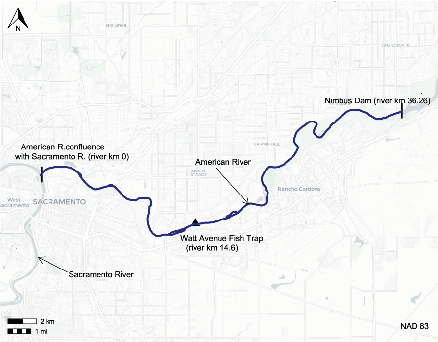
American River locations of Nimbus Dam, Watt Avenue fish trap, and confluence with the Sacramento River, California. [km, kilometer.]
Methods
The three key features of the S3 model relevant to this report are: (1) the estimation of redd and fry Resource Selection Functions (RSFs) to quantify suitable habitat area, (2) the use of habitat estimates with empirical data on river flow and water temperature for the American River, and (3) density-dependent dynamics that are influenced by the effect of flow on suitable habitat area. In this report, we briefly describe the S3 model inputs and outputs as necessary to understand the estimation of redd and juvenile suitable habitat area, as well as the structure of the S3 model and the basic drivers of population dynamics. We encourage readers to consult Perry, Plumb, and others (2018), which details the mathematical structure of the S3 model, and Plumb and others (2019), which provides an example of using S3 simulations to assess the effects of flow and temperature management for the Klamath River, California.
S3. Habitat Template and Physical Inputs
The spatial domain of the S3 model is defined by a one-dimensional representation of discrete habitat units. In total, the American River S3 model comprises 36 river kilometers and has 83 habitat units positioned between Nimbus Dam and the American-Sacramento River confluence. Each habitat unit was classified into one of three mesohabitat types: riffle, run, or pool (Perry and others, 2019). The upper and lower boundaries of the 83 discrete habitat units were assigned based on aerial photographs provided by Google Earth (https://earth.google.com/web/). Using these images, the upper boundary of each habitat unit was measured at the river’s centerline and perpendicular to the shoreline.
The S3 model requires two physical inputs, water temperature and stream flow, that both drive population dynamics directly or indirectly. Water temperature dictates biological rates of development such as maturation of eggs in the gravel and growth of juveniles after emergence. River discharge affects available habitat for juveniles, and in turn, density-dependent dynamics (Perry and others, 2019). We used existing flow and temperature datasets to construct model inputs for the American River S3 model (https://cdec.water.ca.gov/). Because there are no large tributaries to the American River downstream from Nimbus Dam, we used the mean daily discharge at Nimbus Dam to represent the daily flow of the American River in S3 simulations (fig. 2). Although daily average discharge may be a good approximation of flow in the river from Nimbus Dam to its confluence with the Sacramento River, water temperature likely varies along this reach. To account for this, mean daily water temperatures were spatially updated at four locations based on the locations of four temperature measurement stations along the American and Sacramento rivers (fig. 3). From upstream to downstream these stations were (1) Fair Oaks from rkm 36.2 to 21.4, (2) William Pond from rkm 21.4 to 14.5, (3) Watt Avenue Bridge from rkm 14.5 to 6.1, and (4) Sacramento River at Freeport from rkm 6.1 to 0. We used the mean daily temperatures at Freeport because they were likely a more accurate representation of the temperatures of the American River downstream from the Watt Avenue Bridge.
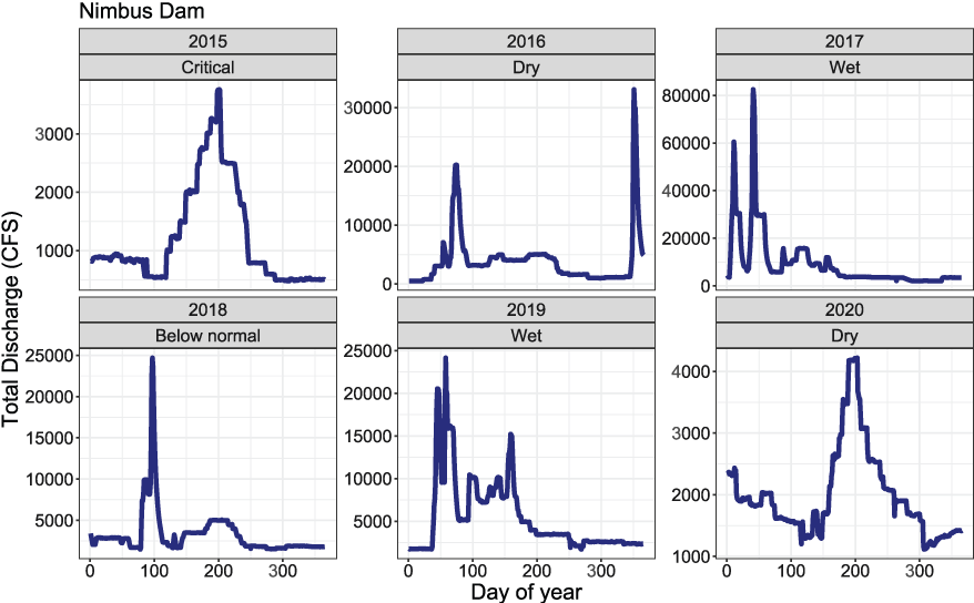
Mean daily discharge for the American River at Nimbus Dam, California, used in Stream Salmonid Simulator model simulations of juvenile Chinook salmon (Oncorhynchus tshawytscha) survival, movement, and consumption, 2015–20. [CFS, cubic feet per second.]
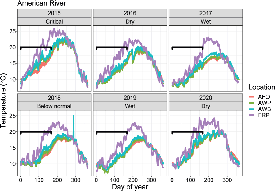
Mean daily temperatures at four locations used to simulate juvenile Chinook salmon (Oncorhynchus tshawytscha) survival, movement, and consumption, on the American River, California, 2015–20. Graphs are shown by outmigration year and water year type for the Sacramento Valley, California. [°C, degrees Celsius; AFO, Fair Oaks; AWP, William Pond; AWB, Watt Avenue Bridge; FRP, Sacramento River at Freeport.]
Estimating Available Habitat
Inputs for the S3 model require relationships between discharge and the amount of suitable habitat at specific life stages within each habitat unit over the model domain. The available habitat area for redd selection and usable fry habitat for each habitat unit was quantified using Resource Selection Functions (RSFs; Manly and others, 1993). The RSFs were then used to scale the weighted usable habitat area constructed from a two-dimensional hydrodynamic model of the American River for each life stage and habitat unit over the S3 model domain (Perry, Plumb, and others, 2018; Perry and others, 2019). This extrapolation procedure was applied to the time series of river flows for each year to develop a time series of available habitat from spawning to emigration.
Obtaining the amount of available habitat for different life stages of juvenile salmon first requires the estimation of the life stage specific RSFs. The methods for estimating the RSF parameters for spawning and juvenile habitat are similar but differ between data sources and model structure. For example, inferences from our RSF estimated from snorkel survey data may only apply to fish less than 55 millimeters (mm) fork length (FL) because our snorkel surveys did not observe fish larger than about 55 mm FL. Therefore, we discuss the different data sources, structure, and methods used to estimate RSF parameters and suitable habitat area for redds, fry, and parr life stages separately.
Available Spawning Habitat
Estimation of RSF parameters for specific life stages requires data on both the presence and absence of those life stages over a range of key habitat conditions. One way to estimate an RSF for redd occurrence is through a logistic regression that includes covariates to estimate the probability of redd occurrence (Manly and others, 1993). Our full RSF model fit to the presence and absence observations of redds (yredd) with all covariate effects (β0-6) was expressed as:
wherep(yredd = 1)
is the probability of redd occurrence;
β0
is the intercept;
β1–4
are quadratic relations to water velocity, V, and water depth, D;
β5
is an interaction between water velocity, V, and water depth, D;
β6
is the effect of distance from the dam;
B
is distance from Nimbus Dam, in meters;
D
is water depth, in meters; and
V
is water velocity, in meters per second.
All covariates were standardized to a mean = 0 and standard deviation (SD) = 1, allowing for direct comparison of effects across the covariate parameter estimates. The mean water velocity was 0.503 meters per second (m/s) (SD = 0.361), the mean depth was 0.846 meters (m) (SD = 0.683), and the mean distance to dam was 7,148.3 m (SD = 6,829.1). We included B, distance from Nimbus Dam, in the model to help capture the phenomenon of higher redd density and spawning below migration barriers.
We used the geospatial locations of fall run Chinook salmon redds obtained by aerial surveys of the American River (Perkins and Hannon, 2021) to estimate the parameters for our RSF of redd occurrence and spawning. Each redd’s geospatial location and the aerial survey date were recorded, enabling the determination of the mean daily river flow at Nimbus Dam (https://cdec.water.ca.gov) for the redds surveyed on a given date. Given these mean daily flows, the geospatial redd locations were matched to the nearest flow stratum provided by the U.S. Army Corps of Engineers using the Hydrologic Engineering Center River Analysis System model (U.S. Army Corps of Engineers, 2023). The HEC-RAS model output was for flow strata of the Lower American River, in cubic feet per second (ft3/s), at: 500, 800, 1,000, 1,250, 1,500, 1,750, 2,000, 2,750, 3,500, 4,500, 5,500, 6,500, 7,500, 8,500, 10,000, 15,000, and 30,000 ft3/s. Because river flows are typically stable, relatively low, and vary little from year to year during the Chinook salmon spawning season, the geospatial redd locations over brood years 2014–19 were matched to the mesh cells from 500 ft3/s (14.2 cubic meters per second [m3/s]) to the 4,500 ft3/s (127.4 m3/s) strata. The cell size of the mesh at each flow strata was provided at a relatively fine scale, having a size of 3 feet (ft) (0.914 m) by 3 ft (0.914 m), or a surface area of 9 square feet (ft2)(0.836 square meters [m2]). If the geospatial location of a redd fell within the given surface area of the mesh cell, then the physical attributes (in other words., depth, velocity, and distance from the dam) of that mesh cell were assigned to that redd observation, providing a dataset of observed redd locations and their associated physical characteristics as determined by the HEC-RAS model output.
Estimation of an RSF requires information on where fish are absent. To obtain absence data, we used methods similar to those of Dudley and others (2020), where bootstrap random samples of cells within a geospatial mesh formed absence observations for estimating an RSF for redds in the Sacramento River, California. Specifically, for a given flow stratum, we sampled 200 times without replacement up to the number of presence observations from the two-dimensional mesh cells where no redds were observed. When cells are matched with the presence of redds, 200 possible datasets were obtained with equal numbers of presence and absence locations, enabling the estimation of the probability of redd occurrence. Like Dudley and others (2020), we tried to minimize the effect of observation bias on our parameter estimates by restricting the sample space of absent mesh cells to a depth less than 10 ft (3 m), which slightly exceeded the maximum depth of the observed redd cells and is typically thought to be a reliable depth expected from aerial surveys (Perkins and Hannon, 2021). Thus, we used the output of the HEC-RAS model to represent the physical conditions at both the redd presence and absence locations. These data were then used to estimate the parameters of the RSF for Chinook salmon redds in the American River.
We fit our 12 candidate RSF models to the 200 bootstrapped datasets and then used Akaike’s Information Criterion (AIC; Burnham and Anderson, 2002) model selection to determine which model structure to use for inference. For each bootstrapped dataset, we calculated the AIC across the 12 models. We then calculated the fraction of times each model had the lowest AIC value over the 200 bootstrapped datasets. The model with the highest fraction of having the lowest AIC value over the 200 bootstrapped samples was chosen for inference and used to calculate the amount of useable redd habitat area. To demonstrate the relative fit of the best AIC model relative to other candidate models, we show the relative difference among the candidate models while using the dataset nearest the mean AIC value. We calculate the model’s predictive accuracy using the Area Under Curve (AUC) and graphical assessments.
We use the parameters for the chosen RSF model to calculate the probability of redd occurrence for each mesh cell in a flow stratum of the HEC-RAS model. The product of a cell’s total area (9 ft2) and its probability of redd selection provides an estimate of the amount of suitable redd habitat area for that cell. At a given flow stratum, summation of the usable habitat area for cells within the boundaries of each habitat unit provides the usable area for redds in each habitat unit. Calculation of the usable habitat area for redds (RUAhf) from the total area (Aihf) of mesh cell, i, in habitat unit, h, at flow strata, f, may be expressed as:
given that Ihf is the total number of HEC-RAS mesh cells within habitat unit, h, at flow strata, f. The estimated values of RUAhf are the dataset used in S3 simulations to accommodate changes in redd habitat over a range in flows for the American River. Habitat units vary in length, so we divide the suitable spawning area for a habitat unit by that habitat unit’s length, resulting in an estimate of the average amount of suitable spawning habitat per meter, making graphical comparison across the habitat units possible.Available Fry Habitat
We took a similar approach to estimate RSF parameters for fry-sized Chinook salmon as we did for redd occurrence. In contrast, the data we used to estimate our fry salmon RSF parameters were obtained from snorkel surveys of the lower American River. We snorkeled about 40 percent (14.3 of the 36 km) of the lower American River between Nimbus Dam and the Sacramento River confluence three times. We recorded 395 geospatial locations of fry Chinook salmon and their associated habitat characteristics such as the approximate numbers of fish, water depth (in meters), and water velocity (in meters per second). We also measured substrate size, distance to nearest cover, and distance to shore. Surveys were conducted daily from March 2 to March 11, 2021, by two independent teams at different locations of the river. Each team consisted of two snorkelers and two habitat assessors. The river was surveyed by the team in either an upstream or downstream direction, depending on accessibility and water currents. Once one or more fish were observed at a location, the number of fry (fish less than 55 mm FL) were estimated by the observer, and the geospatial location and habitat characteristics were measured and recorded. We did not observe juvenile salmon greater than 55 mm FL during our snorkel surveys. For our S3 simulations, we defined the juvenile life stages of Chinook salmon in the American River as fry (FL ≤ 45 mm), parr (45 < FL ≤ 73 mm), and smolt (FL > 73 mm) based on the spectrum of fish sizes passing the Watt Avenue fish trap and recommendations by a coauthor John Hannon (Bureau of Reclamation, Sacramento Office).
The snorkel surveys provided the fish locations, dates, and flows to be compared to the HEC-RAS model. We used the HEC-RAS model to quantify habitat characteristics under flow conditions that occurred during the snorkel surveys (data are currently [August, 2023] available from funding organization Bureau of Reclamation; contact John Hannon with the Bureau of Reclamation, Sacramento, California for further information). The locations of fish during snorkel surveys provided information on fish presence for our RSF model of fry habitat. To obtain data on where fry salmon were absent, we used the same bootstrapped sampling procedure described above for redd presence. We restricted the sample space of absent mesh cells to a depth less than 8 ft, which slightly exceeded the maximum depth that could be sampled by snorkel surveys.
We fit our full RSF to the presence and absence observations of fry salmon, yfry, over the 200 bootstrapped datasets and then used AIC model selection to determine which bootstrapped dataset to use for inference. We chose to base inferences on the bootstrapped sample that produced the mean AIC, such that model fits would not be inadvertently biased when comparing the fit among candidate RSF models. Our full model to estimate the probability of fry presence is:
wherep(yfry = 1)
is the probability of fry presence;
θ0–5
are estimated coefficients for the covariates;
V
is water velocity, in meters per second; and
D
is water depth, in meters.
The probability of fry presence, p(yfry = 1), is a function of the estimated parameters, and quadratic relations to water velocity (V; m/s) and depth (D; m) as well as their linear interaction. All covariates were standardized to mean = 0 and standard deviation (SD) = 1, allowing for direct comparison of effects across the estimated covariate parameters. The mean water velocity was 0.277 m/s (SD = 0.283), and the mean depth was 0.639 m (SD = 0.539).
To decide the parsimonious model among candidate models, we calculate the model that had the highest fraction of having the lowest AIC value across the 200 bootstrapped datasets. The model that had the lowest AIC most often across the bootstrapped datasets was the model we use for inference and habitat estimation for S3 modeling. To demonstrate the relative fit of the best AIC model relative to other candidate models, we show the difference in AIC among the seven models using the dataset nearest the mean AIC value (Burnham and Anderson, 2002). To explore the fit of the RSF, we calculate predicative accuracy using AUC and graphic assessments.
We use the RSF model to calculate the probability of a fry presence for each mesh cell in a flow stratum of the HEC-RAS model. The product of a cell’s total area (about 9 ft2) and the probability of fry presence provides an estimate of the suitable area of habitat for that cell. At a given flow stratum, summation of the suitable habitat area for cells within the boundaries of each habitat unit provides the suitable area for fry salmon in each habitat unit. Calculation of the suitable habitat area for fry salmon (FUAhf; ≤ 45 mm) from the total area (Aihf) of mesh cell, i, in habitat unit, h, at flow strata, f, may be expressed as:
where The estimated values of FUAhf are the data for salmon fry used in S3 simulations to accommodate changes in fry habitat over a range in flows for American River.Available Parr Habitat
We used the habitat suitability indices (HSI) provided by Chris Hammersmaark, CBEC Engineering (written commun., 2019). The HSI ranged from 0 to 1 and was assigned to each HEC-RAS mesh cell. We compare estimates of the HSI from CBEC to our RSF estimates for p(yfry =1). Under the premise that larger juvenile salmon would favor deeper depths than the fry we observed during our snorkel surveys, we used the CBEC HSI values to quantify the suitable habitat area for parr- and smolt-sized fish in the following manner:
wherePUAhf
is the suitable habitat area for parr and smolts;
Ihf
is the total number of HEC-RAS mesh cells within habitat unit h, at flow strata f;
HSIihf
is the CBEC habitat suitability index for each HEC-RAS mesh cell; and
Aihf
is the total area of a mesh cell, i, in habitat unit h, at flow strata f.
These values for each habitat unit and flow stratum were supplied to S3 for simulations and model fitting.
Biological Inputs
The S3 model relies on two primary forms of biological inputs to simulate population dynamics: (1) female spawners and (2) juvenile fish entering from tributaries and hatchery releases. The spatial and temporal distribution of spawners was derived from aerial survey data (Perkins and Hannon, 2021) and weekly escapement estimates from carcass mark-recapture studies (Kelley and Phillips, 2020).
Female Spawners
We used the annual escapement estimates provided by California Department Fish and Wildlife (Kelley and Phillips, 2020), the weekly counts of females (data are available from California Department of Fish and Wildlife; contact Tracy Grimes with the California Department of Fish and Wildlife, Sacramento, California for further information), and aerial surveys of redds (Perkins and Hannon, 2021) to estimate the spatial and temporal distribution of female spawners needed for S3 input. We first estimated the annual fraction of redds (rhy) within each of the 83 designated habitats in the following manner:
whererhy
is the estimated annual fraction of redds within each designated habitat;
nhy
is the number of redds observed in habitat unit, h, out of the total number of redds, Ny, observed during aerial surveys in each year, y; and
Ny
is the total number of redds observed during aerial surveys each year.
Second, we estimated the weekly fraction of females that spawned (ewy) each year in the following manner:
whereewy
is the weekly fraction of female salmon that spawned each year,
carwy
is the weekly count of female carcasses, and
Cary
is the annual count of female carcasses (table 1).
Next, we calculated the total annual number of spawning females (EFy) by taking the product of the total annual escapement, the annual sex ratio, and the annual pre-spawning mortality rate (Perkins and Hannon, 2021). Finally, we calculated the number of weekly female spawners in each habitat unit and year (EFhwy) as:
Table 1.
Annual escapement estimates of spawning female fall-run Chinook salmon (Oncorhynchus tshawytscha) in the American River downstream of Nimbus Dam, California.We subtracted two weeks from the carcass mark-recapture survey weeks to approximate the week the redds were constructed. These counts of redds from female spawners in each habitat unit, week, and year were the input data used to run S3 simulations for the American River.
Juveniles from Hatchery Production
We included hatchery releases of juvenile Chinook salmon as a separate sub-population in S3. Data on Nimbus Hatchery releases of Chinook salmon were obtained from the Regional Mark Information System database (https://www.rmpc.org/). Only juvenile Chinook salmon that were released in the mainstem American River were included in S3. Juvenile Chinook salmon from the Nimbus Hatchery were released in batch releases at boat ramps and public access locations. As a result, each release was associated with a release location and single start and end date. For input to S3, the total number of hatchery fish entering the river each day was the sum of the daily approximated number of fish released. The Nimbus Hatchery also releases cohorts of several other salmonid species throughout the year, but interactions of these salmonids with Chinook salmon are not currently modeled in S3.
In addition to daily hatchery release numbers, S3 requires the mean weight of hatchery fish entering the river. Prior to release, each batch was sampled to estimate the mean weight of the released fish. The mean weight of fish was converted to FL to classify the life stage of hatchery inputs as fry, parr, or smolt upon river entry (table 2). However, the sizes of hatchery juvenile Chinook salmon released into the American River, on average, were smolt-sized fish, less than 73 mm FL.
S3. Submodels and User-Defined Parameter Settings
When simulating fish populations with S3, some population dynamics are dictated via user-defined options and parameter inputs. Juvenile fish populations in the S3 model are affected by three dynamic processes: (1) survival, (2) growth, and (3) movement. We describe how the submodels were parameterized for the American River and specify values of user-defined parameters. For details on the mathematical structure of individual submodels, consult Perry, Plumb, and others (2018).
Spawning, Egg Development, and Egg Survival Submodels
The number of fry emerging from eggs is affected by several S3 parameters and submodels. We set the fecundity of female spawners to 5,291 eggs per redd to approximate the mean number of eggs observed for Chinook salmon returning to the Nimbus Hatchery from 2005 to 2019. The mean time from spawning to fry emergence is modeled as a function of daily water temperature (°C) and the accumulated degree days (see Perry, Plumb, and others, 2018). Variation in emergence timing is assumed to follow a normal distribution about the mean emergence date and is controlled by the standard deviation in degree days required to hatch, which we set to 26.6 days.
During the incubation period, S3 includes three mechanisms that affect egg-to-fry survival: (1) baseline “natural” mortality, (2) temperature-related mortality, and (3) redd superimposition (Perry, Plumb, and others, 2018). The natural mortality rate was set at 0.25 percent per day, which equates to a baseline survival rate of about 92.8 percent per month. Thermal tolerance parameters were set so that water temperatures less than or equal to 17 °C had no effect on egg survival, but temperatures greater than 17 °C imposed a daily mortality rate of 25 percent (Geist and others, 2006).
Redd superimposition is the process whereby a later arriving spawner builds a redd on top of an existing redd and dislodges or entombs the eggs laid by the earlier spawner. Superimposition is modeled in S3 as a function of habitat capacity and spawner abundance. Habitat capacity is the quotient of redd area (obtained from our RSF of redd occurrence) divided by the size of a redd, which was set to 4.5 m2. The probability of redd superimposition is defined by redd density (redd abundance/redd capacity), which is calculated and applied daily for each habitat unit. The amount of redd mortality attributed to superimposition on day t is simply the number of redds to be recruited that day multiplied by the existing pre-recruitment redd density. However, given the propensity of Chinook salmon to guard their redds until death, the S3 model allows the user to define the guarding period. We set the guarding period to 10 days, assuming semelparous Chinook salmon live to guard their nests for 10 days after spawning (see Perry, Plumb, and others, 2018). Redds are not vulnerable to superimposition during the guarding period. Although redd scour owing to freshets is known to influence survival of eggs, we have not yet implemented mortality owing to scour in the S3 model.
Juvenile Growth
We used the Wisconsin Bioenergetics Model in S3 (Perry, Plumb, and others, 2018) to estimate the mean size for each source population and life stage in each habitat unit, which was incremented daily as a function of water temperature, fish body size, and a food consumption rate. The consumption rate can either be assumed or estimated from data. For application to the American River, we took a novel approach compared to past S3 model-fitting efforts that set the consumption parameter to a user-defined fixed value (for example, Perry, Jones, and others, 2018; Perry and others, 2019). We use the mean sizes of fish at the fish trap in the fitting process to estimate the proportion of maximum consumption, Cy, a key growth parameter in the bioenergetics model. We estimate Cy as a time-constant value in S3 simulations from the mean weekly weights of fish at the Watt Avenue fish trap in each year (discussed below). In the past, S3 assumed a constant Cy = 0.66, and to our knowledge, estimation of Cy from field data has never been done within the context of a matrix-based population model before.
The growth model governs life-stage transitions by moving fish to the next life stage when their mean size exceeds user-defined size thresholds for each life stage. For natural-origin fish, we set the weight of emergent fry to 0.3 grams (g) (30 mm FL). The mean size of fry, parr, and smolt were recomputed daily within each habitat unit to account for daily growth, growth-based life-stage transitions, recruitment of emergent fry, and movement among habitat units. We assumed that the growth model applied uniformly to all juvenile life stages, and natural- and hatchery-origin fish populations.
Juvenile Movement
S3 has two submodels for simulating fish movement: (1) the “mover-stayer” model and (2) the “advection-diffusion” model (Perry, Plumb, and others, 2018). In both models, movement from one habitat unit to another is simulated in the downstream direction only. In our simulations, we used the mover-stayer model for rearing fry and parr, and the advection-diffusion model for actively migrating smolts. The mover-stayer model can be implemented with density-independent or density-dependent movement, which is a user-specified option. With density-independent movement, abundance and capacity have no effect on movement probability. Density-independent movement is the only option available with the advection-diffusion model. Perry and others (2019) noted that density-dependent movement fit observed abundance data better than a model with density-dependent survival. Therefore, we chose to fit the model with density-dependent movement to each migration year’s weekly juvenile salmon abundance estimates at the fish trap.
Two parameters drive movement in the mover-stayer model: (1) the probability of remaining in the currently occupied habitat unit (Pstay) from time t to t+1 (resulting in “stayers”), and (2) the mean distance moved downstream (resulting in “movers”; kilometers per day). For the density-dependent form of the model, Pstay is expressed as a Beverton-Holt function (Beverton and Holt, 1993) such that Pstay decreases as the ratio of abundance to capacity increases. That is, the probability of moving (1-Pstay) increases as abundance approaches capacity. Preliminary model fitting indicated that insufficient information was available to estimate capacity through model calibration, so we set capacity to estimates based on Neuswanger and others (2016) and Perry, Jones, and others (2018), where fry capacity was set to 294.9 fish/m2 and parr capacity was set to 94.7 fish/m2. Specifically, during S3 calibration we estimated the intercept, M0y, of the Beverton-Holt function such that Pstay = f(M0y, capacity) for the density-dependent form of the mover-stayer model. The mean distance moved was calculated deterministically as a function of FL (Perry, Plumb, and others, 2018).
We modeled smolt movement using a density-independent advection-diffusion process because this model was developed for actively migrating smolts, not smaller rearing fish that are less likely to move downstream (Zabel and Anderson, 1997; Zabel, 2002). The advection-diffusion model assumes that the spatial distribution of a population at a given point in space after t time units is described by a normal distribution with a mean location and standard deviation. We allow the movement rate of smolts to depend on size, with the rate of movement increasing with fish size. The parameters of this model were based on size relationships developed by Zabel (2002) and Plumb (2012) for juvenile Snake River fall Chinook salmon (Perry, Plumb, and others, 2018).
Juvenile Survival
Daily survival probability, like movement probability, can be specified either as density-independent or density-dependent. In the density-dependent form, survival probability is expressed as a Beverton-Holt function that decreases as the ratio of abundance to capacity increases (Perry, Plumb, and others, 2018). In this form, Sy is the expected survival as abundance approaches zero. In the density-independent form, daily survival probability is estimated as a constant value that does not depend on abundance or habitat capacity. Under both forms of the survival model, parameters may be allowed to differ among life stages and source populations; however, we do not allow the parameters to vary among life stages and source populations in this modeling analysis. Parameters of the survival model were estimated via calibration, which is described below. We use the density-independent form of the survival model in all model fitting in this report. Additionally, we do not allow the parameters to vary among life stages and source populations.
S3. Model Calibration
The goal of calibration is to estimate survival, movement, and growth parameters of the S3 model by fitting the model simultaneously to estimates of weekly abundances and mean sizes (FL) of juvenile salmon passing the rotary screw trap located near the Watt Avenue Bridge. To fit the S3 model to estimated trap abundances and fish sizes, we used the Earth Mover’s Distance (EMD), also known as Mallow’s distance (Levina and Bickel, 2001), between the simulated and estimated distributions of weekly abundances and fish sizes at the fish trap.
Using EMD as a metric to compare congruence between two distributions has several advantages (Levina and Bickel, 2001; Lupu and others, 2017). First, EMD allows for the comparison among multiple dimensions over a time series. The technique has most often been used in pattern recognition and image retrieval (Ling and Okada, 2007), but has been more recently been found to be advantageous whenever multiple distributions are compared (Aggarwal and others, 2001; Lupu and others, 2017). Second, calculation of the EMD is well established, efficient, and tractable, facilitating its use within an optimization framework to estimate survival, movement, and consumption parameters with respect to a time series of fish abundances and sizes.
In our case, for each year, y, we have a matrix, Xy, consisting of two time-series variables: (1) the weekly abundance (Nwy) and (2) the weekly mean size (FLwy) of juvenile salmon passing the fish trap. Correspondingly, we have another matrix, Zy, of weekly abundances () and sizes () of juvenile salmon simulated by S3. These matrices have their respective probability distributions PX and PZ. We calculated the Mallow’s distance between PX and PZ using the emd() function and the ‘emdist’ R software package (Urbanek and Rubner, 2022).
To estimate S3 demographic parameters, we minimized the EMD value with respect to juvenile fish survival, movement, and consumption parameters using the optimization function, optim(), available in R software (R Core Team, 2021). The goal of optimization was to find the combination of parameters that would generate the most similarity between simulated and estimated abundance and fish size distributions. Measuring model fit on an annual basis using EMD (1) allowed multivariate data and thus more information to be included in the fitting process compared to just fitting to abundance alone, (2) better accounted for temporal auto correlation inherent in the time series of trap abundance and sizes, and (3) improved the run time to optimize the S3 parameters to the data over past efforts that fit parameters across years (Perry, Jones, and others, 2018; Perry and others, 2019).
To summarize the fit of the model to the trap data, we visually compare the time series of weekly estimated and simulated abundances and mean weekly fish sizes. We compare abundances by showing the time series of estimated and simulated fish passing the fish trap, as well as to each other (for example, simulated versus estimated). We also compare the total estimated annual abundance at the fish trap to the total annual abundance simulated by S3. We compare mean weekly sizes simulated by S3 to the mean weekly fish sizes and individual sizes of fish observed at the trap. We then contrast the estimated parameters, annual abundances, and juvenile fish sizes by the water year type for the Sacramento Valley (California Department of Water Resources, 2021) of the outmigration year. We also assess the model estimates and output in relation to the abundance of spawning females during the corresponding brood year.
Results
Spawning Habitat Resource Selection Function
Comparisons among the 12 candidate RSF models for redd occurrence supported the full model (model 1) as the best fit model to the data (table 3). Model 2, without the interaction between V and D, had the next-lowest AIC value (difference in AIC value from the lowest AIR model [ΔAIC] = 15.5) to the full model. Both models included distance from the dam, and both had much lower ΔAIC than model 3, which excluded distance to the dam, demonstrating the importance of including distance from the dam in the model. Given these results, we used model 1, the full model, as our RSF for estimating redd occurrence and spawning habitat area for fall Chinook salmon in the lower American River.
Table 3.
Model selection results for 12 candidate Resource Selection Functions to determine redd site selection for fall-run Chinook salmon (Oncorhynchus tshawytscha) in the American River, California.[Results are based on the bootstrapped dataset that was nearest the mean Akaike’s Information Criterion (AIC) over the 200 bootstrapped datasets. The model covariates are velocity (V), depth (D), and distance from Nimbus Dam (B). K, number of model parameters; NLL, negative log-likelihood; AIC, Akaike’s Information Criterion for the model; ∆AIC, difference in AIC value from the lowest AIC model]
Assessment of model fit indicated that the best RSF model for redd occurrence (model 1) fit the data well. The best model (deviance = 17,212) explained 47 percent of the null deviance (32,677). The model also had good predictive accuracy and an ability to discriminate among used and unused redd sites, having an AUC = 0.89. For perspective, perfect predictability is AUC = 1 and random chance is AUC = 0.5. Graphically comparing the fit of a spline model to the probabilities from the RSF provide a qualitative representation of model fit over the range of each covariate (fig. 4). The predicted trend and values for the spline and the RSF model for redd occurrence were in good agreement.
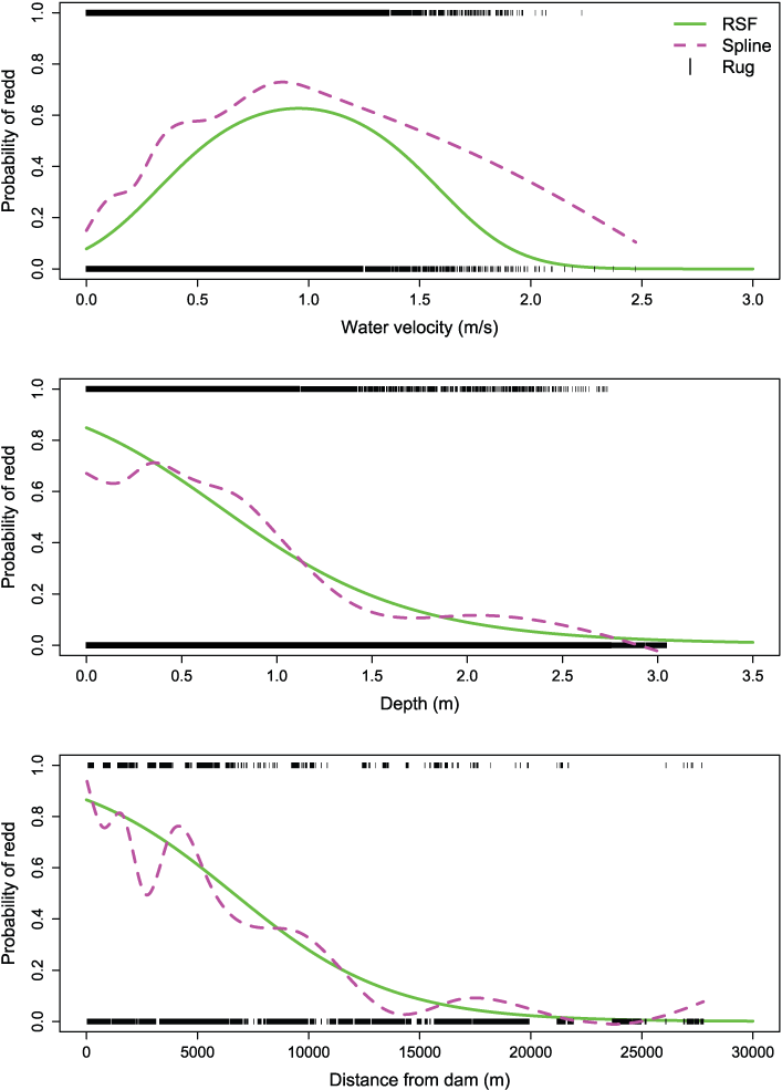
Estimated effects of water velocity, depth, and distance from Nimbus Dam on probability of redd occurrence for Chinook salmon (Oncorhynchus tshawytscha), American River, California. The rug plot shows the observed presence (value of 1) and absence (value of 0) of redds, the dashed magenta line represents the fit of a spline model to these data to illustrate the fit of the more parsimonious Resource Selection Function (RSF) model (solid green line). [m/s, meters per second; m, meters.]
Comparison among model covariates indicated that the effect of distance to the dam was the most influential and negative (β6 = –1.918) with lower redd occurrence as the distance from Nimbus Dam increased (table 4; fig. 4). There was support for including a quadratic effect of water depth (β3 = –1.418) with greater redd occurrence from about 0.01 to 0.5 m. The quadratic effect of water velocity was dynamic with high redd occurrence from about 0.75 to 0.95 m/s.
Table 4.
Coefficient estimates and their standard errors for the Akaike’s Information Criterion best model (Model 1) used to estimate redd site selection for Chinook salmon (Oncorhynchus tshawytscha) in the American River, California.[Coefficient: The effects (β1-6) for water velocity (V, in meters per second), depth (D, meters), and distance to Nimbus Dam (B, in meters)]
We illustrate the estimated change in usable spawning area over a range in flows for pools, riffles, and runs. Regardless of habitat unit type, we measured peaks in the relative usable spawning area at river flows from 1,000 to 6,000 ft3/s (fig. 5). Riffle habitats typically provided higher usable area over the range in flows than either pools or runs. At high flows greater than 25,000 ft3/s, pool and run habitat types had similar usable habitat area per unit length.
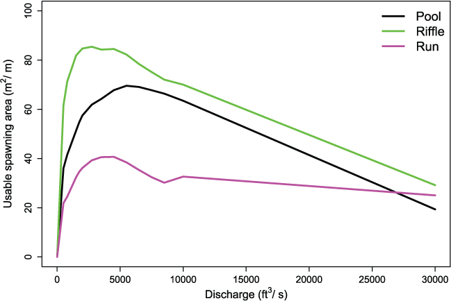
Estimated changes in usable spawning area over a range in flows for three different habitat units located a few kilometers downstream from Nimbus Dam, on the American River, California. The pool is at river kilometer (rkm) 34.49, the riffle is at rkm 34.05, and the run is at rkm 33.95. [m2/m, square meters per meter; ft3/s, cubic feet per second.]
Fry Resource Selection Functions
Comparisons among six candidate RSF models for fry occurrence supported Model 2, with quadratic effects of water velocity (V) and depth (D), as the best fit model to the data. (table 5). Model 1, with the interaction effect between V and D was 2.00 ΔAIC from Model 2, suggesting the interaction contributed little to model fit. Model 3, without quadratics and an interaction, was 17.75 ΔAIC from Model 2 and fit the data worse than Model 4 without the interaction term (ΔAIC = 15.76). The difference in AIC values between Models 2 and 4 demonstrate the importance of including a quadratic structure in the model. Given these results, we used the quadratic model, Model 2, as the RSF for estimating juvenile presence and usable habitat for fall Chinook salmon fry in the lower American River.
Table 5.
Model selection results for six candidate Resource Selection Functions to determine juvenile habitat for Chinook salmon (Oncorhynchus tshawytscha) in the American River, California.[Results are based on the bootstrapped dataset that was nearest the mean AIC over the 200 bootstrapped datasets. Table shows the model number, model structure, the number of parameters (K), the negative log-likelihood (NLL), the AIC value, and the difference in AIC value from the lowest AIC model (ΔAIC)]
The fry RSF model fit the data well. The RSF (deviance = 17,212) explained 32 percent of the null deviance (920.4). The model also has good predictive accuracy and an ability to discriminate among the presence and absence of fry, having an AUC = 0.84. Comparing the fit of a spline model to the RSF provides a qualitative comparison of the juvenile RSF’s fit and trend over the range of each covariate (fig. 6). The predicted trend in the spline model and the RSF were in good agreement.
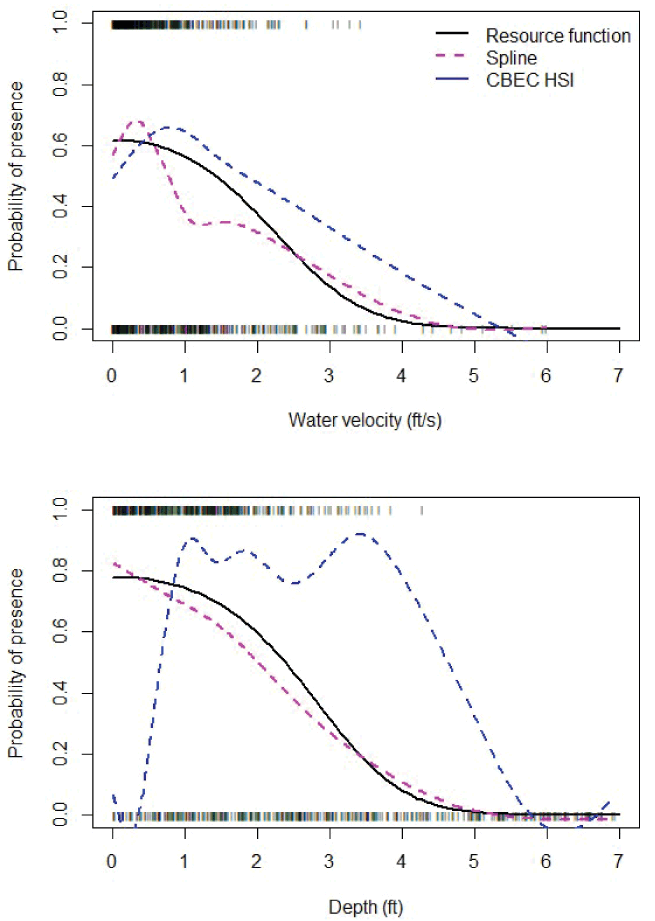
Estimated effects of the fry Resource Selection Function based on snorkel surveys and two-dimensional hydrodynamics model output. The rug plot shows the observed presence (value of 1) and absence (value of 0) of fry, the magenta dashed line represents the fit of a spline model to these data to illustrate the more parsimonious fit of the Resource Selection Function model (Resource function, solid black line). Also shown is the blue dashed line of the fit of the spline model to the habitat suitability indices (CBEC HSI) used for parr habitat provided by CBEC Engineering. [ft/s, feet per second; ft, feet.]
The effect of water depth was the most influential (Ɵ3 = –1.716) with higher fry presence at shallow depths between 0.01 and 0.5 m (table 6; fig. 6). Water velocity was quadratic (Ɵ1 = –0.409) with greater probability of fry presence between about 0.01 and 0.5 m/s. The quadratic effect of water velocity was apparent with higher habitat selection from about 0.75 to 0.95 m/s. Thus, the small fish (< 55 mm) we observed in the field generally selected slow water velocities and shallow depths.
Table 6.
The quadratic effects (Ɵ1-4) of water velocity (V; meters per second) and depth (D; meters) and their standard errors for the Akaike’s Information Criterion best model (Model 2) used to estimate juvenile habitat for Chinook salmon (Oncorhynchus tshawytscha) in the American River, California.Parr Habitat Suitability
The estimates of juvenile habitat selection between our RSF and the HSI values provided by CBEC showed similar trends with respect to water velocity (fig. 6). However, the CBEC estimates favored deeper water depths than our RSF that was estimated from snorkel surveys. Given that larger sized fish would be more likely to choose deeper water depths than those we observed during snorkel surveys, we thought it was prudent to use CBEC’s HSI values to obtain habitat area for parr and smolt size fish in S3 simulations.
Dividing the usable juvenile habitat area by each habitat unit’s length provides the amount of usable parr habitat area per linear meter of river, facilitating comparison of suitable habitat area across habitat units and types (fig. 7). Regardless of habitat unit type, we measured peaks in the relative suitable parr habitat area at river flows between 100 and about 2,500 ft3/s. Pool habitats provided higher suitable area over the range in flows for fry- and parr-sized fish, but riffles provided a relatively large amount of suitable habitat area for fry at relatively low flows. On a per meter basis, there was about twice as much suitable habitat estimated for parr as for fry.
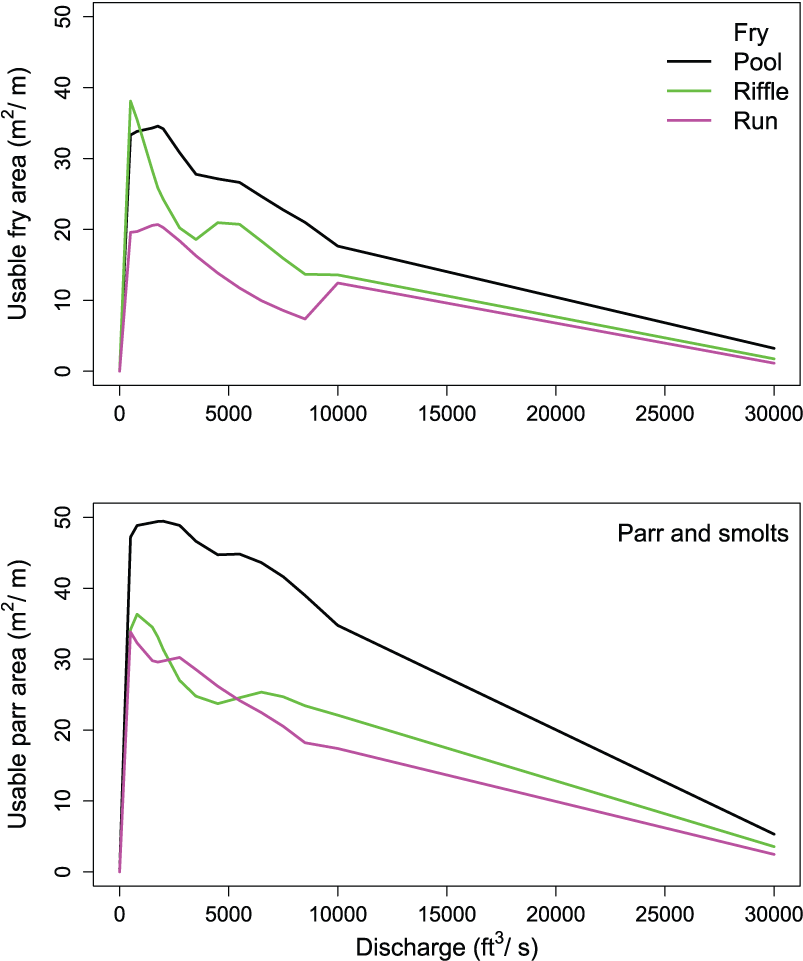
Change in usable habitat for juvenile Chinook salmon (Oncorhynchus tshawytscha) over a range in flows for three different habitat units located downstream from Nimbus Dam, on the American River, California. The pool was at river kilometer (rkm) 34.49, the riffle at rkm 34.05, and run at rkm 33.95. [m2/m, square meters per meter; ft3/s, cubic feet per second.]
S3. Model Calibration
Survival, Movement, and Consumption Parameters
Minimizing the EMD with respect to the survival, movement, and consumption parameters yielded a best-fit set of S3 parameters to simulate the weekly abundances in each year (table 7). Annual daily survival probabilities (Sy) ranged from Sy = 0.739 to Sy = 0.932, with lower Sy associated with high spawner abundances and critical to dry water year types (figs. 8 and 9). To put these daily survival estimates in perspective, the highest Sy in 2019 results in 49.6 percent of the population surviving after 10 days, and the lowest Sy in 2015 results in 4.8 percent of the population surviving after 10 days. Thus, even our highest Sy is low when viewed over longer temporal scales.
Table 7.
Daily survival, movement, and consumption parameter estimates obtained by minimizing the Earth Mover’s Distance (EMD) with respect to the parameter set and the weekly trap abundance estimates for each migration year.[Movement is defined as the daily probability of remaining in a habitat unit, and consumption is the proportion of maximum consumption as defined in the Wisconsin bioenergetics model (Perry, Plumb, and others, 2018). Also shown is the water year type during the migration year, and the spawner abundance during the previous brood year]
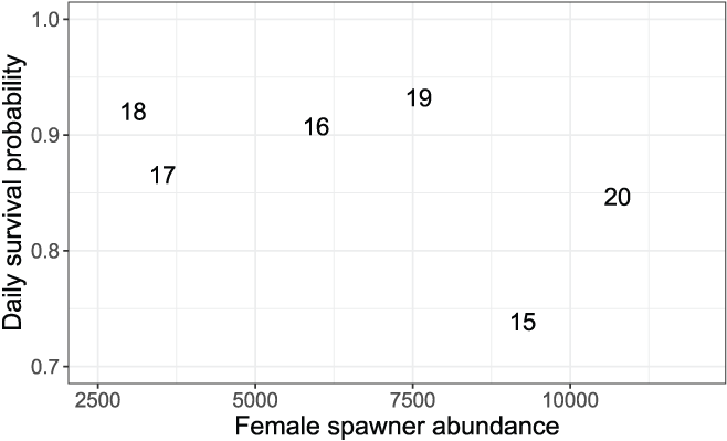
Daily survival probabilities and the number of female spawners during the previous brood year. The data points are the last two digits of each migration year.
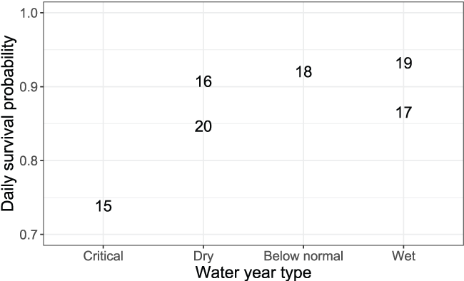
Daily survival probabilities by water year type during the juvenile Chinook salmon (Oncorhynchus tshawytscha) outmigration. The data points are the last two digits of each migration year.
The intercepts of the Beverton-Holt model, M0y, for the probability of remaining in a habitat ranged from 0.010 in 2017 to 0.634 in 2019 (table 7, “Movement” column). We found no consistent pattern in M0y over the range in spawner abundances (fig. 10), although this is not surprising, given that we fit the density-dependent movement model, which should account for effects of fish density on fish movement. There was a trend towards higher M0y (that is, greater site fidelity at low abundance) with wetter water year types (fig. 11). The exception to this pattern was the low M0y in the extremely wet year of 2017, suggesting that at very high flows fish were emigrating rapidly regardless of fish density, compared to other years.
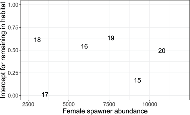
Estimated intercepts of the Beverton-Holt model for density-dependent movement in juvenile fall-run Chinook salmon (Oncorhynchus tshawytscha), in the American River, California. Movement is defined as the probability of remaining in a habitat unit at near zero abundances, which are plotted on the number of female spawners during the previous brood year. The data points are the last two digits of each migration year.
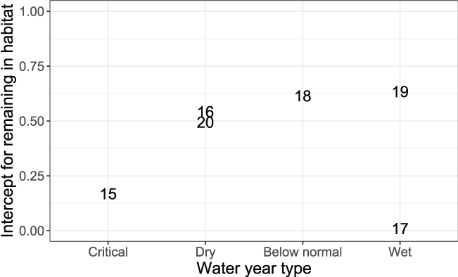
Estimated intercepts of the Beverton-Holt model for density-dependent movement in juvenile fall-run Chinook salmon (Oncorhynchus tshawytscha), in the American River, California. Movement is defined as the probability of remaining in a habitat unit at near zero abundances., which are plotted on the water year type for the Sacramento Valley. The data points are the last two digits of each migration year.
Daily proportions of maximum consumption were relatively high (Cy > 0.837) except during 2017 when fish were estimated to eat just 10.4 percent of their expected maximum consumption (table 7). Thus, during the extremely wet year of 2017, fish moved the fastest and consumed the least. When the high-water year of 2017 is excluded, there was a trend toward higher daily proportions of maximum consumption at higher spawner abundances (fig. 12), and lower daily proportions of maximum consumption from dry to wet water years (fig. 13). Estimates of daily proportions of maximum consumption were greater than that previously assumed for S3 simulations where Cy = 0.66.
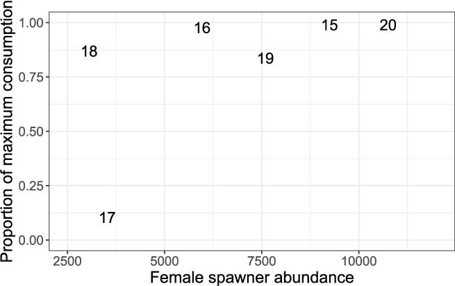
Daily average proportions of maximum consumption plotted on the number of female Chinook salmon (Oncorhynchus tshawytscha) spawners during the previous brood year. The data points are the last two digits of each migration year.
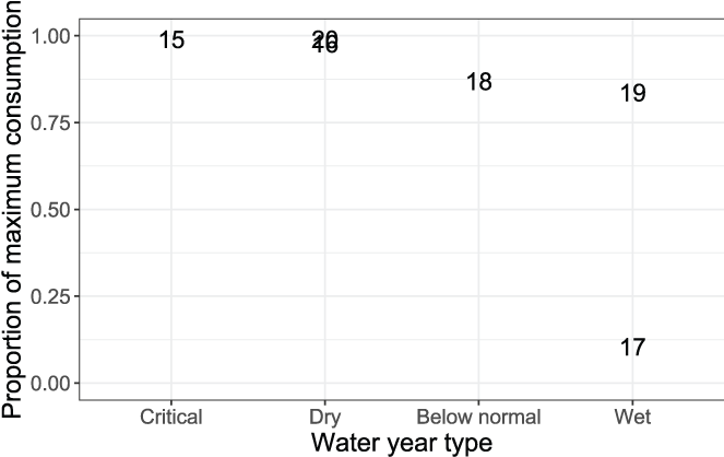
Daily average proportions of maximum consumption by water year type during the juvenile Chinook salmon (Oncorhynchus tshawytscha) outmigration. The data points are the last two digits of each migration year.
Fish Abundance and Size
The S3 model simulated the annual abundances quite well (fig. 14). When plotted against each other, the estimated and simulated annual abundances were close to the 1:1 line of equality. This finding confirms that our fitting process estimated the total annual abundances for each year quite well.
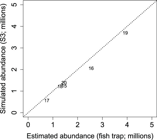
Estimated and simulated Stream Salmonid Simulator annual abundances of juvenile Chinook salmon (Oncorhynchus tshawytscha) at the Watt Avenue fish trap, American River, California. Data points represent the last two digits of the migration year, and the dashed line is the line of equality.
Comparison of estimated to simulated weekly abundances of fish passing the Watt Avenue fish trap indicated that the S3 model was missing some important within-year effects important to juvenile salmon migration (fig. 15). The general timing of migration was captured by S3, but simulations often over-predicted troughs or under-predicted peaks in the weekly abundances of fish passing the trap each year. Thus, it was apparent that just three parameters estimated as annual constants were not sufficient to describe the within-year outmigration of juvenile Chinook salmon. Plotting the estimated and simulated trap abundances passing the Watt Avenue fish trap demonstrated the fit of the S3 model to the weekly abundance estimates (fig. 16). On the observed scale, a heteroscedastic pattern was apparent; however, increasing error might be expected with increasing abundance. When plotted on the log scale, the larger outliers were apparent at high estimated but low simulated weekly abundances.
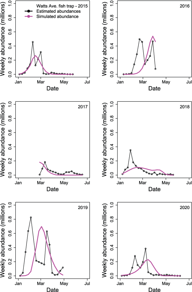
Weekly time series of abundances of juvenile Chinook salmon (Oncorhynchus tshawytscha) by migration year passing the Watt Avenue fish trap when estimated from the trap catch (black line and points) or simulated by the Stream Salmonid Simulator model (magenta line), in the American River, California, 2015–20.
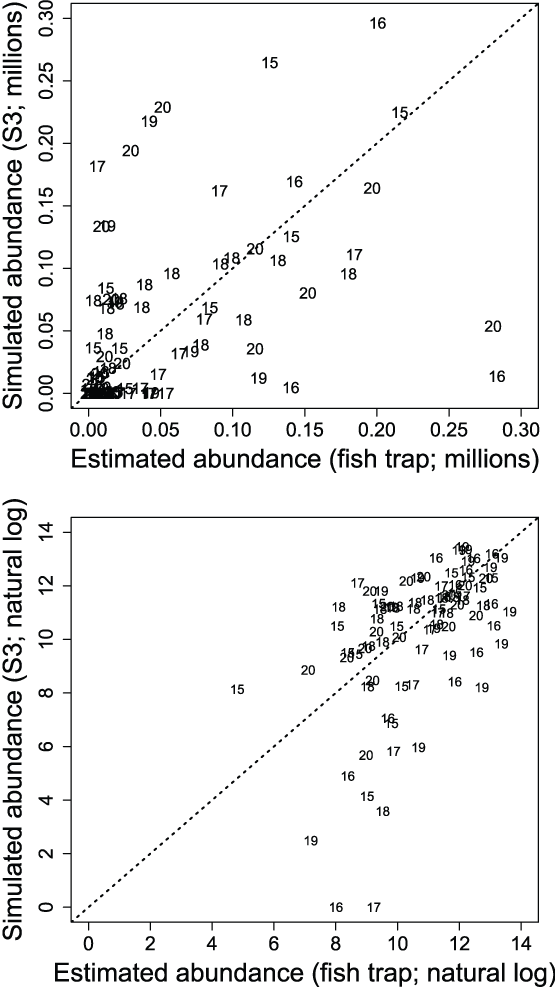
Estimated and simulated Stream Salmonid Simulator weekly abundances of juvenile Chinook salmon (Oncorhynchus tshawytscha) at the Watt Avenue fish trap, American River, California. The upper graph is on the observed scale and the bottom graph is on the log scale. Data points represent the last two digits of the migration year, and the dashed line is the line of equality.
The S3 model simulated the general trend in fish sizes and life-stage transitions over the time series (fig. 17). However, we found lack of fit in mean weekly FL in years that also showed a marked lack of fit in weekly abundances (figs. 17 and 18). For example, in migration year 2016, S3 tended to overestimate the mean weekly size of fish at the trap, and in 2015 underestimated the mean weekly FL (fig. 18). Overall, S3 was able to capture the trend in fish growth within each year. Because we fit the S3 model to the time series of both abundance and size, improvement in model fit to fish size may best be achieved by matching weekly abundances (fig. 15).
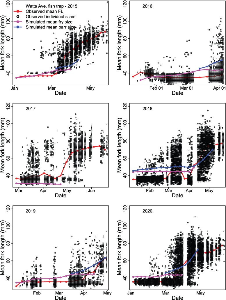
Time series of juvenile Chinook salmon (Oncorhynchus tshawytscha) fork lengths (FL) at the Watt Avenue fish trap during each migration year, in the American River, California, 2015–20. The black dots are observed FL of individual fish and the red line is the observed mean weekly FL. The Stream Salmonid Simulator simulated FL are shown for fry (magenta line) and parr (blue line) life stages. [mm, millimeters.]
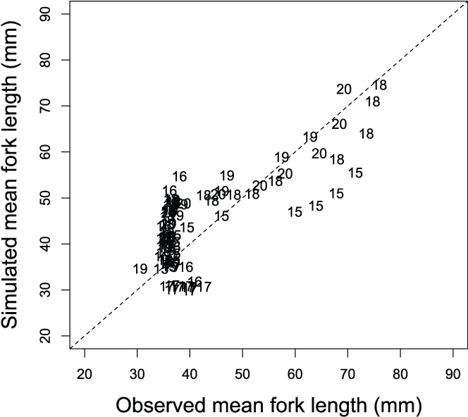
Mean weekly fork lengths of juvenile Chinook salmon (Oncorhynchus tshawytscha) at the Watt Avenue fish trap, American River, California, plotted against the Stream Salmonid Simulator simulated mean weekly fork lengths, 2015–20. The data points are the last two digits of each migration year. [mm, millimeters.]
Simulated Spawning, Emergence, and Abundance
Naturally Produced Juvenile Salmon
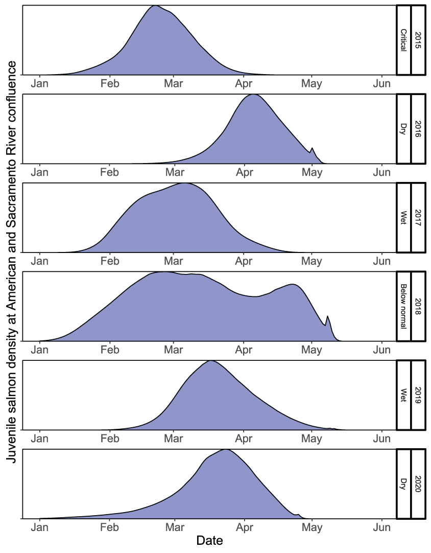
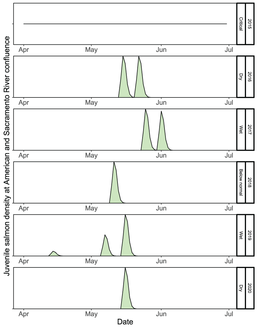
Given the calibrated parameters to the Watt Avenue fish trap, the temporal distribution of spawning females sets up the initial conditions to which the simulated eggs and juveniles will be exposed during emigration. Although the intervening temperatures during egg incubation affect the rate of egg maturation, the timing of fry emergence was dictated by the timing of spawning and the time series of water temperatures (figs. 19 and 20). Survival during egg incubation ranged from 0.674 to 0.756 (table 8). There was no apparent pattern in incubation survival over the annual time series because egg maturation times were similar among years and temperatures did not exceed 17 °C during the egg incubation period. In contrast, the survival of emerging juveniles to the Sacramento confluence ranged from 0.01 to 0.072 (table 8), which confirms low survival of simulated fish from brood years with high spawner abundances and critical to dry years during migration. The total annual number of naturally produced juveniles to arrive at the Sacramento River confluence ranged from 333,356 to 1,927,011 (table 8). Emigration timing of the simulated natural fall run Chinook salmon was also a reflection of the spawning and emergence timing, such that later spawning resulted in later emergence, and in turn, a later emigration (fig. 21). Over the annual time series, juvenile salmon entered the Sacramento River from January to the first week of May.
Table 8.
Survival during egg incubation and survival and abundance to the American-Sacramento River confluence for natural and hatchery produced juvenile Chinook salmon (Oncorhynchus tshawytscha) in the American River, California, as simulated by the Stream Salmonid Simulator model.[No hatchery-reared fish were released into the American River in 2015. --, not applicable]
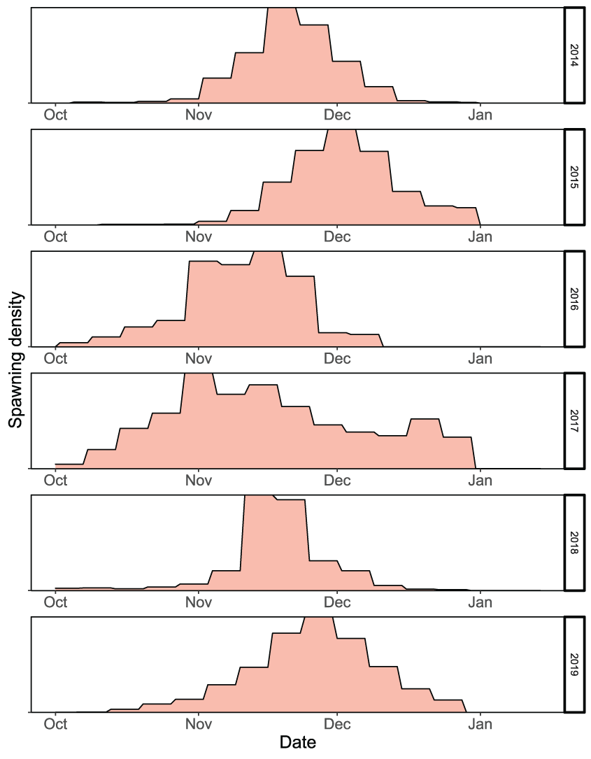
Spawn timing of female fall run Chinook salmon (Oncorhynchus tshawytscha) by brood year used to simulate the emergence and emigration of juvenile salmon in the lower American River, California, 2014–19.
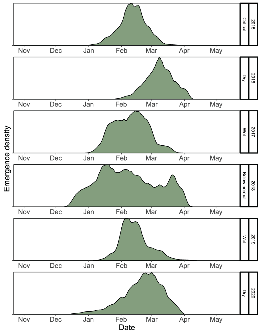
Emergence timing of fall run Chinook salmon (Oncorhynchus tshawytscha) fry, by migration year and water year type, in the lower American River, California, 2015–20.
Run timing of simulated natural fall run Chinook salmon (Oncorhynchus tshawytscha) juveniles released, by migration year and type, into the lower American River, California, 2015–20.
Hatchery Produced Juvenile Salmon
Hatchery juvenile salmon released into the lower American River were simulated using the same parameter values as the natural juvenile salmon, but the fish were released at much larger sizes later in the migration season. Because of their much larger size than the natural fish, the simulated hatchery fish emigrated rapidly during May and early June (fig. 22). No hatchery fish were released in the lower American River during the critically dry year of 2015. Owing to their relatively rapid migration rates, the survival of simulated hatchery fish to the confluence with Sacramento River ranged from 0.847 to 0.925 (table 8). Although hatchery and natural fish were simulated to have the same daily survival probability (Sy), the higher simulated survival of hatchery fish to the Sacramento River confluence was the result of their larger size resulting in faster migration rates and less time for mortality to occur.
Run timing of simulated hatchery fall run Chinook salmon (Oncorhynchus tshawytscha) juveniles released, by migration year and water year type, into the lower American River, California, 2015–20.
Discussion
Choosing the American River for application the S3 was a successful decision because of the rich and available supply of necessary habitat, physical, and biological input data, making calibration and simulation of the model to the fish trap data possible. The S3 model was designed as a tool for use in a Decision Support System for rivers with ongoing management concerns (for example, the Trinity River Restoration Program; Perry, Jones, and others, 2018). Likewise, this report presents the first step in using the S3 model to provide information to a Decision Support System in congruence with the FISH plan that was initiated for the lower American River in 2001.
Because S3 can be used to formulate and test hypotheses about river-management options, we have identified several areas that could improve the model’s performance and future application. First, on the data side, only estimates of total abundance and average fish size were available, so estimates of abundance and fish size for specific fry, parr, and smolt life stages could help inform the model-fitting procedure and allow for the estimation of life stage-specific parameter estimates. Second, external information from acoustic telemetry or passive integrated transponder tag studies could be used to measure juvenile fish survival and migration rates independently from model calibration, and when incorporated in S3 indirectly allow for the estimation of survival during egg incubation. Finally, including addition covariates on fish movement within S3 might help explain juvenile salmon population dynamics. For example, the effect of lunar illumination has been correlated with trap catch. Biologists operating the Watt Avenue fish trap anticipate the amount of effort needed based on the fraction of lunar illumination (Logan Day, Pacific States Marine Fisheries Commission, oral commun., 2021) Although S3 does not currently include lunar effects on fish movement, doing so could greatly improve model fit and its utility as a tool to compare among hypothesized scenarios (app.1, Figure 1.1). Because S3 fit the estimated annual abundances so well, including within-year lunar effects on fish movement seems the most plausible and cost-effective means for improving the model’s fit to observed weekly abundance estimates.
Caution should be used when making inferences from S3 parameter estimates in relation to spawner abundances and water year types. The parameters obtained by fitting S3 simulations to trap abundances and fish sizes is an indirect approach to estimating survival, movement, and consumption parameters that dictate juvenile salmon population dynamics. For example, trap abundance estimates to which we fit the S3 model are not perfect because catchability of fish traps can be influenced by river flow. Our daily survival estimates also are quite low, resulting in as little as 5 percent and as much as 50 percent survival over just 10 days. However, because S3 assumes a relatively high daily survival rate during egg incubation (Segg = 0.9975), estimates of daily survival could be biased low if egg survival is lower than S3 currently assumes. Alternatively, tagging studies could provide S3 with direct estimates of juvenile survival and movement, in which case survival during egg incubation could be estimated indirectly via model fitting. Therefore, we caution against drawing much inference from the differences in the annual S3 parameter estimates.
Given this caution, however, we identified sensible patterns over the annual parameter values, spawner abundances, and water year types. Our most outlying parameter estimate was during the extremely high flow year of 2017. For very wet years, both M0y and Cy were lowest, suggesting that fish moved out quickly with little opportunity for consumption and growth at low abundances. Excluding 2017, a trend from dry to wet water year types was associated with higher values of M0y, yet a slight decline in Cy, suggesting that from dry to wet years there may be less density-dependence in movement at low fish abundance. Yet, average daily consumption relative to maximum consumption may be lower during wetter conditions. Nonetheless, except for the extremely wet year of 2017, proportions of maximum consumption were generally quite high (> 0.84), suggesting that the fish caught by the juvenile trap fed at relatively high consumption rates (for example, see Armstrong and Schindler, 2011). Interestingly, we also measured our lowest daily survival during the critically dry migration year of 2015, which could support density-dependence in fish survival, and a potential avenue for future research. Thus, many of the trends and differences in parameter values among the years make sense when compared among water years and spawner abundances.
This report represents the first iteration of using the S3 model as a framework for research and management of the lower American River, and with each iteration we learn more about the S3 model’s limitations and strengths. The S3 model offers the opportunity to integrate biological and physical characteristics over the entire temporal and spatial freshwater residency of juvenile salmonid populations. As such, the S3 model can provide valuable insights into the potentially variable impacts that different management decisions may have in the American River. Combinations of system attributes (for example, physical habitat, hydrographs, and temperatures) subject to manipulation by managers can be translated into scenarios that form the inputs for S3 model runs. The S3 model has the potential to provide more accurate predictions of absolute abundance by estimating life stage-specific abundances at the traps, incorporating information from independent studies on egg or juvenile survival and migration rates, and further model development and hypothesis testing to determine variables important to juvenile salmon during their outmigration. S3 model output may be useful when comparing relative differences of population demographics such as fish abundance, size, and run timing across pre-specified scenarios. These predictions, in turn, will inform a broader management objective (as well as model development), and in turn, will complete the adaptive management loop, leading to a refined management decision process for the benefit of the American River.
References Cited
Beverton, R.J.H., and Holt, S.J., 1993, On the dynamics of exploited fish populations: Dordrecht, Springer, 538 p. [Also available at https://link.springer.com/book/10.1007/978-94-011-2106-4.]
CALFED Bay-Delta Program, 1999, Ecosystem restoration program plan, strategic plan for ecosystem restoration—Draft programmatic environmental impact statement/environmental impact report technical appendix: Prepared for the United States Bureau of Reclamation, United States Fish and Wildlife Service, National Marine Fisheries Service, United States Environmental Protection Agency, Natural Resources Conservation Service, United States Army Corps of Engineers, and California Resources Agency, published by Congressional Research Service, Sacramento, California, p. 1–14.
California Department of Water Resources, 2021, California Data Exchange Center: California Data Exchange Center web page, accessed December 2021, at https://cdec.water.ca.gov.
Geist, D.R., Abernethy, S.C., Hand, K.D., Cullinan, V.I., Chandler, J.A., and Groves, P.A., 2006, Survival, development, and growth of fall Chinook salmon embryos, alevins, and fry exposed to variable thermal and dissolved oxygen regimes: Transactions of the American Fisheries Society, v. 135, no. 6, p. 1462–1477.
Neuswanger, J.R., Wipfli, M.S., Rosenberger, A.E., and Hughes, N.F., 2016, Measuring fish and their physical habitats—Versatile 2D and 3D video techniques with user-friendly software: Canadian Journal of Fisheries and Aquatic Sciences, v. 73, no. 12, p. 1861–1873, accessed October 1, 2018, at https://cdnsciencepub.com/journal/cjfas.
Perry, R.W., Jones, E.C., Plumb, J.M., Som, N.A., Hetrick, N.J., Hardy, T.B., Polos, J.C., Martin, A.C., Alvarez, J.S., and De Juilio, K.P., 2018, Application of the Stream Salmonid Simulator (S3) to the restoration reach of the Trinity River, California—Parameterization and calibration: U.S. Geological Survey Open-File Report 2018–1174, 64 p. [Also available at https://doi.org/10.3133/ofr20181174.]
Perry, R.W., Plumb, J.M., Jones, E.C., Som, N.A., Hardy, T.B., and Hetrick, N.J., 2019, Application of the Stream Salmonid Simulator (S3) to Klamath River fall Chinook salmon (Oncorhynchus tshawytscha), California—Parameterization and calibration: U.S. Geological Survey Open-File Report 2019–1107, 89 p. [Also available at https://doi.org/10.3133/ofr20191107.]
Perry, R.W., Plumb, J.M., Jones, E.C., Som, N.A., Hetrick, N.J., and Hardy, T.B., 2018, Model structure of the stream salmonid simulator (S3)—A dynamic model for simulating growth, movement, and survival of juvenile salmonids: U.S. Geological Survey Open-File Report 2018–1056, 32 p. [Also available at https://doi.org/10.3133/ofr20181056.]
Plumb, J.M., 2012, Evaluation of models and the factors affecting the migration and growth of naturally produced subyearling fall Chinook salmon (Oncorhynchus tshawytscha) in the lower Snake River: Doctoral dissertation, Moscow, Idaho, University of Idaho, p 1–153. [Also available at https://www.researchgate.net/publication/259601672_EVALUATION_OF_MODELS_AND_THE_FACTORS_AFFECTING_THE_MIGRATION_AND_GROWTH_OF_NATURALLY-PRODUCED_SUBYE ARLING_FALL_CHINOOK_SALMON_ONCORHYNCHUS_TSHAWYTSCHA_IN_THE_LOWER_SNAKE_RIVER.]
Plumb, J.M., Perry, R.W., Som, N.A., Alexander, J., and Hetrick, N.J., 2019, Using the Stream Salmonid Simulator (S3) to assess juvenile Chinook salmon (Oncorhynchus tshawytscha) production under historical and proposed action flows in the Klamath River, California: U.S. Geological Survey Open-File Report 2019–1099, 43 p. [Also available at https://doi.org/10.3133/ofr20191099.]
Prager, M.H., and Mohr, M.S., 2001, The harvest rate model for Klamath River fall Chinook salmon, with management applications and comments on model development and documentation: North American Journal of Fisheries Management, v. 21, no. 3, p. 533–547. [Also available at https://mhprager.com/reports/Prager_Mohr_2001_KHRM_NAJFM.pdf.]
R Core Team, 2021, R—A language and environment for statistical computing: Vienna, Austria, R Foundation for Statistical Computing software release, accessed August 3, 2020, at https://www.R-project.org/.
Surface Water Resources, Inc., 2001, Aquatic resources of the lower American River—Baseline report (draft): Prepared for the Lower American River Fisheries and Instream Habitat (FISH) working group by Surface Water Resources, Inc., [variously paged], accessed June 2021 at https://www.noaa.gov/sites/default/files/legacy/document/2020/Oct/07354626214.pdf.
Urbanek, S. and Rubner, Y., 2022, Earth mover’s distance, An R function: version 3.1, accessed January 2023, at https://cran.r-project.org/web/packages/emdist/emdist.pdf.
U.S. Army Corps of Engineers, 2023, Hydrologic Engineering Center River Analysis System (HEC-RAS): U.S. Army Corps of Engineers Hydrologic Engineering Center web page, accessed January 2023, at https://www.hec.usace.army.mil/.
Winship, A.J., O’Farrell, M.R., and Mohr, M.S., 2012, Management strategy evaluation for Sacramento River winter Chinook salmon, 85 p. [Also available at https://www.pcouncil.org/documents/2007/10/management-strategy-evaluation-for-sacramento-river-winter-chinook-salmon.pdf.]
Zeug, S.C., Bergman, P.S., Cavallo, B.J., and Jones, K.S., 2012, Application of a life cycle simulation model to evaluate impacts of water management and conservation actions on an endangered population of Chinook salmon: Environmental Modeling and Assessment, v. 17, no. 5, p. 455–467 [Also available at https://www.waterboards.ca.gov/waterrights/water_issues/programs/bay_delta/docs/cmnt091412/rosenfeld/5zeug.pdf.]
Appendix 1. Additional Figures
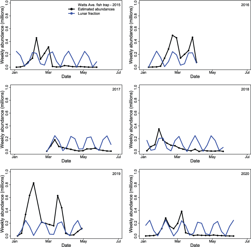
Graphs showing weekly time series of abundances of juvenile Chinook salmon (Oncorhynchus tshawytscha) by migration year passing the Watt Avenue fish trap when estimated from the trap catch (black line and points) and the fractions of the moon that were illuminated (blue line), in the American River, California, 2015–20. Note that the fraction of lunar illumination was scaled to 25 percent of the value for comparative purposes.
Conversion Factors
Abbreviations
∆AIC
difference in AIC value from the lowest AIC model
AIC
Akaike’s Information Criterion
AUC
area under curve
CBEC
CBEC Engineering
EMD
Earth Mover’s Distance
FISH
Fisheries and Instream Habitat
FL
fork length
HEC-RAS
Hydrologic Engineering Center River Analysis System
HSI
Habitat Suitability Index
RCMP
River Corridor Management Plan
rkm
river kilometer
RSF
Resource Selection Function
S3
Stream Salmonid Simulator
For information about the research in this report, contact
Director, Western Fisheries Research Center
U.S. Geological Survey
6505 NE 65th Street
Seattle, Washington 98115-5016
https://www.usgs.gov/centers/wfrc
Manuscript approved on August 2, 2023
Publishing support provided by the U.S. Geological Survey
Science Publishing Network, Tacoma Publishing Service Center
Disclaimers
Any use of trade, firm, or product names is for descriptive purposes only and does not imply endorsement by the U.S. Government.
Although this information product, for the most part, is in the public domain, it also may contain copyrighted materials as noted in the text. Permission to reproduce copyrighted items must be secured from the copyright owner.
Suggested Citation
Plumb, J.M., Perry, R.W., Hatton, T.W., Smith, C.D., and Hannon, J.M., 2023, Application of the Stream Salmonid Simulator (S3) model to assess fall Chinook salmon (Oncorhynchus tshawytscha) production in the American River, California: U.S. Geological Survey Open-File Report 2023–1060, 35 p., https://doi.org/10.3133/ofr20231060.
ISSN: 2331-1258 (online)
Study Area
| Publication type | Report |
|---|---|
| Publication Subtype | USGS Numbered Series |
| Title | Application of the Stream Salmonid Simulator (S3) model to assess fall Chinook salmon (Oncorhynchus tshawytscha) production in the American River, California |
| Series title | Open-File Report |
| Series number | 2023-1060 |
| DOI | 10.3133/ofr20231060 |
| Publication Date | October 11, 2023 |
| Year Published | 2023 |
| Language | English |
| Publisher | U.S. Geological Survey |
| Publisher location | Reston, VA |
| Contributing office(s) | Western Fisheries Research Center |
| Description | ix, 35 p. |
| Country | United States |
| State | California |
| Other Geospatial | American River |
| Online Only (Y/N) | Y |