

California State Waters Map Series—Benthic Habitat Characterization in the Region Offshore of Morro Bay, California
Links
- Document: Report (5 MB pdf) , HTML , XML
- Data Releases:
- USGS Data Release - Bathymetry, backscatter intensity, and benthic habitat offshore of Morro Bay, California
- USGS Data Release - Bathymetry, backscatter intensity, and benthic habitat offshore of Point Estero, California
- USGS Data Release - Bathymetry, backscatter intensity, and benthic habitat offshore of Point Buchon, California
- NGMDB Index Page: National Geologic Map Database Index Page (html)
- Download citation as: RIS | Dublin Core
Acknowledgments
This report was prepared in cooperation with the Bureau of Ocean Energy Management and the California Ocean Protection Council. The California Ocean Protection Council funded the acquisition of data used in this study during the California Seafloor Mapping Program. The Bureau of Ocean Energy Management (BOEM) funded data analysis for this study under Intra-agency Agreement M17PG00021. The report was prepared in collaboration with California State University Monterey Bay and the University of California Santa Cruz.
Multibeam echo sounder data were collected by Fugro, Inc., the U.S. Geological Survey Pacific Coastal and Marine Science Center, and the California State University Monterey Bay Seafloor Mapping Laboratory. The authors thank the science parties, and the crews of all three mapping entities for the mapping carried out during this study. Towed bottom-video camera data were collected by the Humboldt State University R/V Coral Sea. The authors thank the Captain, Scott Martin, the crew of the vessel, and the watch-standers who logged observations of geology and biota during the surveys. Olivia Cheriton (USGS) and James Conrad (USGS) provided helpful peer reviews.
Abstract
Coastal and Marine Ecological Classification Standard geoform, substrate, and biotic component geographic information system products were developed for the California State waters of south-central California in the region offshore of Morro Bay. The study was motivated by interest in development of offshore wind-energy capacity and infrastructure in Federal waters offshore. The Bureau of Ocean Energy Management, in coordination with the State of California and many other members of the California Intergovernmental Renewable Energy Task Force, issued calls for information in 2018 for the study area offshore of Morro Bay, California. The study area is adjacent to a nuclear power plant (currently scheduled for decommissioning) with a developed electric grid connection, and in an area of high wind resource potential. The Bureau of Ocean Energy Management is the lead agency responsible for planning and leasing in the U.S. Exclusive Economic Zone and funded this project to assess baseline conditions of, and the potential effects on, the seafloor environment. This project, carried out by the U.S. Geological Survey, resulted in three data releases for individual map blocks that are part of the California State Waters Map Series: (1) Offshore of Point Estero, (2) Offshore of Morro Bay, and (3) Offshore of Point Buchon. The study area consists of 341 square kilometers (km2) of multibeam echo sounder (MBES) data acquired by Fugro, Inc., in 2010. Towed camera-sled video was acquired in 2012 to supervise the classification of the MBES data into habitats. There were 935 annotations of organisms and habitat made from 22 video transects. Using video observations of habitat as ground truth, derivatives of the MBES data were classified into 3 seafloor character types (hard-rugged, hard-flat, and soft-flat), 25 modifier groups, and 9 geoforms. The study area substrate is predominantly soft-flat sediment (mud and fine sand) covering 191.3 km2 (56.1 percent) of the area. Hard-flat substrate areas, predominantly coarse sediment in scour depressions, cover 52.2 km2 (15.3 percent) of the study area. The hard-rugged substrate areas are primarily outcrops of layered sedimentary bedrock and constitute 97.5 km2 of the study area (28.6 percent). After classification of bathymetry and backscatter raster images according to substrate, false-positive hard areas produced by noise artifacts were removed by manual editing. Nine geoforms were then identified in the analysis. The predominant geoforms mirror the seafloor character results, shelf geoforms (flat areas covered in soft sediment), rock outcrop geoforms (hard, rugged areas), and scour depression geoforms (flat areas covered in coarse sediment formed by bottom currents).
Introduction
This analysis was motivated by interest from private companies and State and Federal government agencies to develop offshore wind energy capacity and infrastructure. The potential direct, indirect, and cumulative effects on the human, coastal, and marine environments are evaluated by the Bureau of Ocean Energy Management (BOEM) to make environmentally sound decisions about managing energy activities. Offshore wind development has the potential to affect the seafloor over large areas and thus BOEM has a critical need for seafloor mapping and habitat characterization. This information will enable a baseline assessment of the area’s seafloor conditions and habitats, which is requisite for subsequent evaluations of the changes and effects to the seafloor from offshore wind development operations. As a companion research agency in the U.S. Department of the Interior, the U.S. Geological Survey (USGS) is mandated with providing Earth-science data acquisition and interpretation to provide baseline data to assess geology and habitat in BOEM regions of interest. BOEM, in coordination with the State of California and many other members of the California Intergovernmental Renewable Energy Task Force, issued two calls for information in 2018 for the study area (Bureau of Ocean Energy Management, 2018). The study area is in California State waters adjacent to a nuclear power plant (currently scheduled for decommissioning) with a developed electric grid connection, and in an area of high wind resource potential (fig. 1).
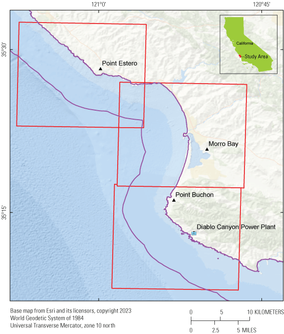
Map showing the three California Seafloor Mapping Program blocks in the study area offshore of Morro Bay, California—Offshore of Point Estero, Offshore of Morro Bay, and Offshore of Point Buchon. Red rectangles are the three map blocks discussed in this report. Purple lines indicate the boundaries of California state waters.
In 2007, the California Ocean Protection Council initiated the California Seafloor Mapping Program (CSMP), which was designed to create a comprehensive seafloor map of high-resolution bathymetry, marine benthic habitats, and geology within California’s State waters. The program supports many coastal-zone- and ocean-management issues, including the California Marine Life Protection Act (California Department of Fish and Wildlife, 2008), which requires information about the distribution of ecosystems as part of the design and proposal process for the establishment of Marine Protected Areas. A focus of CSMP is to map California’s State waters with consistent methods at a consistent scale.
The CSMP approach was to create highly detailed seafloor maps through collection, integration, interpretation, and visualization of swath sonar bathymetric and backscatter data (either multibeam echosounder or bathymetric sidescan sonar), seafloor video, seafloor photography, high-resolution seismic-reflection profiles, and bottom-sediment sampling data. The map products display seafloor morphology and character, identify marine benthic habitats, and illustrate the surficial seafloor geology and shallow subsurface geology. It is emphasized that the habitat and geological models rely on the integration of multiple, high-resolution datasets and that mapping at small scales would not be possible without such data.
The CSMP approach is based in part on recommendations of the Marine Mapping Planning Workshop (Kvitek and others, 2006), which was attended by coastal and marine managers and scientists from around the State. That workshop established geographic priorities for a coastal mapping project and identified the need for coverage of “lands” from the shore strand line (defined as Mean Higher High Water; MHHW) out to the limit of California’s State waters. Surveying the zone from MHHW to 10-meter (m) water depth, however, is not consistently possible using ship-based surveying methods, owing to sea state (for example, waves, wind, or currents), kelp coverage, and shallow rock outcrops. Accordingly, some of the maps presented in this series do not cover the zone from the shore to 5–10 m depth.
Data acquired for this study included multibeam echo sounder (MBES) data (fig. 2) and towed camera-sled video data. The MBES mapping covered a total of 341 km2 and was conducted by Fugro, Inc., in 2008 as part of the California Seafloor Mapping Program (Johnson and others, 2017). Towed camera sled operations were carried out by USGS from 2008 to 2012.
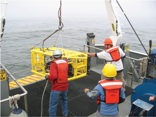
Photograph of camera sled being launched for ground-truth survey transect. U.S. Geological Survey photograph by Guy R. Cochrane, July 16, 2009.
This report discusses the methods used and the mapping and habitat characterization products produced by the USGS for the study area, including a seafloor character raster (Cochrane, 2008) and a Coastal and Marine Ecological Classification Standard (CMECS) polygon shapefile map with geoform and biotic component attributes (Federal Geographic Data Committee [FGDC], 2012). These mapping products are available from Cochrane and others (2022a, b, c) so that they can be incorporated into geographic information system (GIS) and statistical analysis projects.
The geographic scope of this study is focused on the south-central part of California State waters in the region offshore of Morro Bay. Potential wind-energy developers indicated interest in areas offshore at depths of 500 to 1,200 m, far enough offshore to access higher wind potential and to reduce conflicts that could occur closer to shore. Cabling and other infrastructure to connect to the power grid, however, would necessarily pass through California State waters. Previous high-resolution mapping in the area of interest was carried out by the California Seafloor Mapping Program (Johnson and others, 2017) on continental shelf areas; however, there had been no analysis of the data in this part of the continental shelf offshore of south-central California. The intent of this study is to inform and provide regional context for future site-specific surveys.
Methods
The methodological approach used to characterize the physical benthic habitat in the study area was used previously for the California Ocean Protection Council funded project on the California continental shelf (Golden, 2013; Johnson and others, 2017). Multibeam echo sounder (MBES) bathymetry and backscatter data were acquired and used to design a towed camera-sled seafloor video ground-truth survey. Physical habitat and biota were cataloged during the video survey and subsequently used to supervise the classification of the MBES data into physical habitat models.
Multibeam Echo Sounder Surveys
MBES data (with backscatter intensity information) were acquired in the south-central California region by Fugro, Inc., in 2008, using a combination of 400-kHz Reson 7125, 240-kHz Reson 8101, and 100-kHz Reson 8111 multibeam echo sounders. During the Fugro, Inc., mapping missions, an Applanix position and orientation system for marine vessels (POS-MV) was used to accurately position the vessels during data collection, and it also accounted for vessel motion such as heave, pitch, and roll, with navigational input from GPS receivers. Smoothed Best Estimated Trajectory (SBET) files were postprocessed from logged POS-MV files. Sound-velocity profiles were collected with an Applied Microsystems (AM) SVPlus sound velocimeter. Soundings were corrected for (1) vessel motion using the Applanix POS-MV data, (2) variations in water-column sound velocity using the AM SVPlus data, and (3) variations in water height (tides) and heave using the postprocessed SBET data (California State University, Monterey Bay, Seafloor Mapping Laboratory, 2016).
The backscatter-intensity data were postprocessed using Geocoder software. The backscatter intensities were radiometrically corrected (including despeckling and angle-varying gain adjustments), and the position of each acoustic sample was geometrically corrected for slant range on a line-by-line basis. After the lines were corrected, they were mosaicked into 0.5-m resolution images (California State University, Monterey Bay, Seafloor Mapping Laboratory, 2016).
Within the final imagery, brighter tones indicate higher backscatter intensity, and darker tones indicate lower backscatter intensity. The intensity represents a complex interaction between the acoustic pulse and the seafloor, as well as characteristics within the shallow subsurface, providing a general indication of seafloor texture and composition. Backscatter intensity depends on several factors, including the acoustic source level, the frequency used to image the seafloor; the grazing angle, the composition and character of the seafloor, including grain size, water content, bulk density, and seafloor roughness; and some biological cover. Harder and rougher bottom types such as rocky outcrops or coarse sediment typically return stronger intensities (high backscatter, lighter tones), whereas softer bottom types such as fine sediment return weaker intensities (low backscatter, darker tones).
In 2021, the University of California Santa Cruz Center for Integrated Spatial Research imported the bathymetry and backscatter intensity mosaics into an ArcGIS 10 GIS project, where they were mosaicked and clipped into a single tag image file format mosaics for data releases for each block (Cochrane and others, 2022a, b, c).
Video Survey
To validate the interpretations of sonar data to turn them into geologically and biologically useful information, the U.S. Geological Survey (USGS) towed a camera sled (fig. 2) in 2012 over specific locations throughout the study area to collect video and photographic data to ground truth, or visually supervise, the classification of the MBES data into seafloor habitat units. The camera sled was towed 1 to 2 m above the seafloor, at speeds of between 0.5 and 2.0 nautical miles per hour (nm/h). Ground-truth surveys in this map area include approximately 22.6 trackline kilometers (km) of video and 9,227 still photographs, in addition to 934 recorded seafloor observations of abiotic and biotic attributes. A visual estimate of slope also was recorded.
During the ground-truth survey cruises, the USGS camera sled housed two standard-definition (640×480-pixel resolution) video cameras (one forward looking, and one downward looking), as well as a high-definition (1,080×1,920-pixel resolution) video camera and an 8-megapixel digital still camera. In addition to the video recording of the seafloor characteristics, a digital still photograph was captured once every 30 seconds.
The camera-sled tracklines (shown by black dots on the map in fig. 3) are sited to visually inspect areas representative of the full range of bottom hardness and ruggedness in the map area. The video was fed in real time to the research vessel, where USGS and National Oceanic and Atmospheric Administration (NOAA) scientists recorded the geologic and biologic character of the seafloor. While the camera was deployed, several different observations were recorded for a 10-second period once every minute, using the protocol of Anderson and others (2007). Observations of primary substrate, secondary substrate, slope, abiotic complexity, biotic complexity, and biotic cover were mandatory for every observation. Observations of key geologic features and the presence of key species also were recorded when observed.
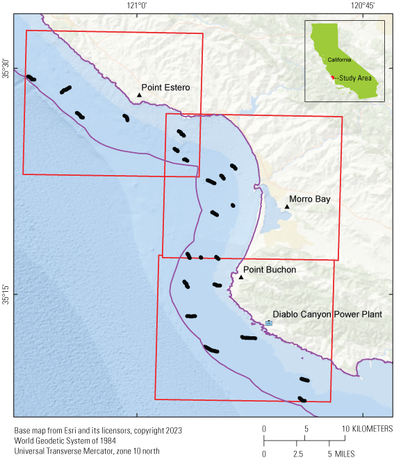
Map showing locations of video observations (black dots) of substrate and other attributes used for analysis for this study in the region offshore of Morro Bay, California. Video was acquired during U.S. Geological Survey field activity C0212SC. Red rectangles are the three map blocks discussed in this report. Purple lines indicate the boundaries of California state waters.
Primary and secondary substrate, by definition, constitute greater than 50 and 20 percent of the seafloor, respectively, during an observation. The grain-size values that differentiate the substrate classes are based on the Wentworth (1922) scale, and the sand, cobble, and boulder sizes are classified as in Wentworth (1922). However, the difficulty in distinguishing the finest divisions in the Wentworth (1922) scale during video observations made it necessary to aggregate some grain-size classes, as was done in the Anderson and others (2007) methodology—the granule and pebble sizes have been grouped together into a class called “gravel,” and the clay and silt sizes have been grouped together into a class called “mud.” In addition, hard bottom and clasts larger than boulder size are classified as “rock.” Benthic-habitat complexity, which is divided into abiotic (geologic) and biotic (biologic) components, refers to the visual classification of local geologic features and biota that potentially can provide refuge for both juvenile and adult forms of various species (Tissot and others, 2006). The video used in this study was acquired on USGS field activity C0212SC, the video can be viewed in Golden and Ackerman (2015), and the observations are published as a point shapefile (Golden, 2013).
Substrate observations were translated into seafloor character classes by USGS for use as classification supervision (table 1). From this information, it is possible to supervise a final classification of the substrate and terrain for the entire mapped area. The substrate model is intended for use in developing species and biotope distribution models using the associations developed between biota and the physical habitat attributes.
Table 1.
Morro Bay State waters region study area video observation combinations and the seafloor character value assigned to the seafloor (fig. 4).[A primary substrate type is considered to cover 50 percent or more of the area in view; the secondary substrate type covers an area greater than 20 percent and less than 50 percent. Substrate grain-size categories are based on those of Wentworth (1922). A value of both in the “Megaripple” column means ripples and megaripples were observed]
Seafloor Character Classification
The California State Marine Life Protection Act calls for protecting representative types of habitat in different depth zones and environmental conditions. A science team, assembled under the auspices of the California Department of Fish and Wildlife (CDFW), identified seven substrate-defined seafloor habitats in California’s State waters that can be classified using sonar data and seafloor video and photography. These habitats include rocky banks, intertidal zones, sandy or soft ocean bottoms, underwater pinnacles, kelp forests, submarine canyons, and seagrass beds. The following five depth zones, which determine changes in species composition, have been identified: depth zone 1, intertidal; depth zone 2, intertidal to 30 m; depth zone 3, 30–100 m; depth zone 4, 100–200 m; and depth zone 5, greater than 200 m (California Department of Fish and Wildlife, 2008). The CDFW habitats can be considered a subset of the broader CMECS classification scheme.
A 2007 Coastal Map Development Workshop, hosted by the USGS in Menlo Park, California, identified the need for more detailed (relative to CMECS or Greene and others’ [1999] attributes) raster products that preserve some of the transitional character of the seafloor when substrates are mixed and (or) they change gradationally. The seafloor-character map, which delineates a subset of the CDFW habitats, is a GIS-derived raster product that can be produced in a consistent manner from data of variable quality covering large geographic regions. The seafloor character raster is a three-substrate classification suitable for inclusion in statistical analyses for species distribution models and other habitat management issues. The seafloor character raster is based on the MBES bathymetry and backscatter data and preserves the resolution of those rasters allowing a one-to-one stacking of the rasters in an analysis stack. The three substrate classes are (1) soft (mud and fine sand), (2) hard-flat (coarse sand, gravel, cobble, and low relief rock outcrop), and (3) hard-rugged (boulder, megaclast, and rugged rock outcrop). The seafloor character classification was produced using video-supervised maximum likelihood classification (MLC) of the bathymetry and backscatter intensity from the MBES survey, following the method described by Cochrane (2008). For each California State University Monterey Bay survey, an MLC was run using the backscatter and vector ruggedness measurement. The vector ruggedness measurement calculation was performed using the Terrain Ruggedness tool within the Benthic Terrain Modeler toolset v. 3.0 (Walbridge and others, 2018). The ground-truth video observation points informed the design of this polygon supervision shapefile. The polygon training sites were selected on the basis of the ground-truth video observations in low-noise MBES areas, where applicable, or otherwise they were selected using best judgment. MLC outputs were iterated, and training sites modified until an acceptable accuracy was achieved. Accuracies are based on an agreement between the predicted class where there is a video observation of the substrate of 80 percent or greater. Accuracies are reported in the three data releases associated with this area (Cochrane and others, 2022a, b, c).
Noise in the bathymetry data was classified as areas of false highs and lows that the numerical analysis converts into areas of ruggedness. The backscatter intensity shows false high-low-backscatter stripes that the numerical analysis converts into stripes in the classified raster. Hand editing in ArcGIS Pro also was done to remove noise artifacts and a majority filter was used to eliminate any remaining small areas of less than three pixels.
Coastal and Marine Ecological Classification Standard Polygons
Shapefiles consisting of polygons around areas of unique combinations of raster variables were produced for each block in the study area and are available in the companion data releases (Cochrane, 2022a, b, c). The shapefiles are attributed with CMECS geoform, substrate, and modifier component values. Each component is represented in the shapefile by a CMECS code and a description from the CMEC standard (FGDC, 2012).
The modifier component is a direct translation of the seafloor character raster classes, and derivatives of the bathymetry raster into the polygons; the modifier variable in the shapefile encodes CMECS induration, slope, and depth class. The induration is derived from the seafloor character raster class. The CMECS induration code scheme (where hard has a value of 3, mixed is 2, and soft is 1) is the reverse of the seafloor character coding. The slope is classified into CMECS slope classes that exist in this dataset—flat (0–5 degrees), sloping (5–30 degrees), and steeply sloping (30–60 degrees). The depth is classified into zones that exist in the dataset— shallow infralittoral (0–5 m), deep infralittoral (5–30), and circalittoral (30–200 m). The CMECS codes come from a technical guidance document (Marine and Coastal Spatial Data Subcommittee, 2014). For example, a hard (sediment induration class 1), steeply sloping (slope class 3) area with depths ranging from 5 to 30 m (benthic depth zone 3) would have a modifier code of SI1S3BDZ3.
The geoform component polygon attribute values were derived from a combination of bathymetric position index (BPI), slope, and induration classes (table 2). The BPI raster was classified into concave, convex, and flat areas. Several geoforms were either too large or too subtle to delineate with BPI. Tar mounds and pockmarks were initially classified as rock outcrops and depressions respectively and were manually reattributed.
Table 2.
Geoform classification attribute values.[BPI, bathymetric position index]
Results
The seafloor character raster map (fig. 4) shows that the study area substrate is predominantly soft-flat, which is interpreted as mud and fine-grained sand, and occupies 95.7 square kilometers (km2)(56.1 percent) of the study area. Hard-flat substrate areas around rocky outcrops and the adjacent shelf are interpreted to be areas of coarse sediment formed by bottom current scour; they make up 26.1 km2 (15.3 percent) of the study area. Hard-rugged substrates are interpreted to be bedrock outcrops and make up 48.8 km2 of the study area (28.6 percent).
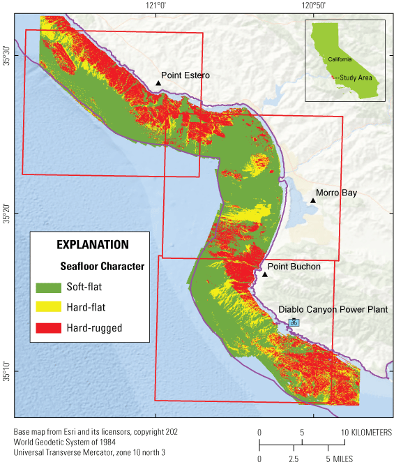
Map showing seafloor character raster image offshore of Morro Bay, California. Red rectangles are the three map blocks discussed in this report. Purple lines indicate the boundaries of California state waters.
The CMECS tectonic and physiographic settings of the study area are transform continental margin and continental shelf. There are 27 unique combinations of variables resulting in 865,562 CMECS polygons in the study area. These polygons are grouped into 25 modifier groups (table 3) and 9 geoforms (fig. 5, table 4). The combinations of modifiers differentiate areas of different induration, slope, and depth. Sand substrate areas were assigned to both soft-flat induration or hard-flat induration class based on the CMECS induration numerical classification derived, in part, from the backscatter intensity data. The soft steeply sloping modifier groups are likely artifacts of MBES noise that were not edited out of the rasters during the manual editing effort. Erroneous mixed and hard steeply sloping areas are likely as well.
Table 3.
The 25 combinations of Coastal and Marine Ecological Classification Standard (CMECS) modifiers identified in the offshore of Morro Bay, California, study area with their total areas of coverage.[km2, square kilometer]
Table 4.
Coastal and Marine Ecological Classification Standard (CMECS) geoforms identified in the offshore of Morro Bay, California, study area with their total areas of coverage.[Geoforms are available as a polygon attribute in the companion data releases (Cochrane and others, 2022a, b, c). km2, square kilometer]
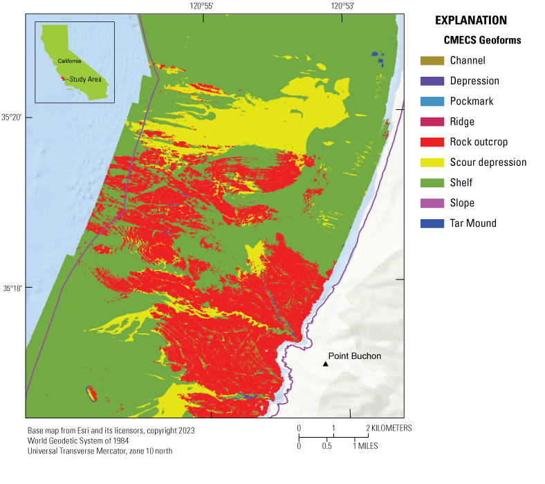
Map showing Coastal and Marine Ecological Classification Standard (CMECS) geoform boundaries offshore of Point Buchon, California. Purple lines indicate the boundaries of California state waters.
The geoform composing the largest area in the region is the shelf geoform (57.4 percent, table 4). The shelf areas are flat, soft sediment covered areas with sediment deposits thick enough to support infauna. The second most extensive geoform is rock outcrop (27.4 percent, table 4). Rock outcrop areas appear to be outcrops of Miocene sedimentary rock (Isaacs, 1981), which are seen extensively in California State waters. These are folded, faulted, dipping, and differentially eroded layered rocks that provide excellent habitat for structure-seeking benthic biota. Tar mounds and pockmarks are located in a small, nearshore, area directly off the city of Morro Bay. The presence of tar seeps and pockmarks typically associated with methane seepage are likely related to the presence of the Miocene sedimentary rocks which are known to be petroliferous (McCulloch, 1987). Geoforms labeled as “Ridge” on figure 5 are convex areas that are both soft and mixed induration and differ from rock outcrop geoforms, which are areas of hard induration.
Scour depression geoforms constitute 13.8 percent of the study area and were assigned on the basis of the observation of one or more of a group of features that include both larger scale bedform (for example, sand waves) fields, as well as coarse sediment-filled depressions that resemble both the rippled scour depressions of Cacchione and others (1984) and the sorted bedforms of Murray and Thieler (2004). These areas are believed to be formed by strong bottom currents flowing from the nearshore to the offshore during storms or high wave activity periods. Scour depression areas are observed in the small interstices formed by fracture or differential erosion of the sedimentary rock outcrops. Where these interstices contain soft sediment, they are classified as depression geoforms.
Table 5 shows the biotic classes logged during video operations. The logging was done with a programmable keypad using the method of Anderson and others (2007). Physical habitat observations were recorded simultaneously as described in the “Methods” section. The combination of biotic and habitat observations could be used to statistically derive biotic groups in the future, but more video data would probably be needed to generate species or biotic-group distribution models.
Table 5.
Summary attributes of biotic classes logged during video operations in the study area offshore of Morro Bay, California.[Biota limited to California Seafloor Mapping Program keypad list of attributes. Depth minimum and maximum are to seafloor and listed in meters]
Summary
Coastal and Marine Ecological Classification Standard geoform, substrate, and biotic component geographic information system products were developed for the California State waters of south-central California in the region of Morro Bay. This analysis was motivated because of interest by private companies and government at all levels to develop offshore wind energy capacity and infrastructure. The potential direct, indirect, and cumulative effects on the human, coastal, and marine environments are evaluated by the Bureau of Ocean Energy Management to make environmentally sound decisions about managing energy activities.
This project, carried out by the U.S. Geological Survey, resulted in three data releases for individual map blocks that are part of the California State Waters Map Series—Offshore of Point Estero, Offshore of Morro Bay, and Offshore of Point Buchon. The study area consists of 341 square kilometers (km2) of multibeam echo sounder (MBES) data acquired by Fugro, Inc., in 2010. Towed camera-sled video was acquired in 2012 to supervise the classification of the MBES data into habitats, and 935 annotations of organisms and habitat were made from 22 video transects. Using video observations of habitat as ground truth, derivatives of the MBES data were classified into 3 substrate induration types, 25 modifier groups, and 9 geoforms. The study area substrate is predominantly soft-flat sediment (mud and fine sand) covering 191.3 km2 (56.1 percent) of the area. Hard-flat substrate areas, predominantly coarse sediment in scour depressions, constitute 52.2 km2 (15.3 percent) of the study area. Hard-rugged substrate areas are outcrops of layered sedimentary bedrock and constitute 97.5 km2 of the study area (28.6 percent). Nine geoforms were identified in the analysis. The predominant geoforms mirror the substrate induration results, shelf (flat areas covered in soft sediment), rock outcrop, and scour depression (flat areas covered in coarse sediment formed by bottom currents). The shelf geoform constitutes 57.4 percent, rock outcrop constitutes 27.4 percent, and scour depression geoforms constitute 13.8 percent of the study area.
References Cited
Anderson, T.J., Cochrane, G.R., Roberts, D.A., Chezar, H., and Hatcher, G., 2007, A rapid method to characterize seabed habitats and associated macro-organisms, in Todd, B.J., and Greene, H.G., eds., Mapping the seafloor for habitat characterization: Geological Association of Canada Special Paper 47, p. 71–79.
Bureau of Ocean Energy Management, 2018, Commercial leasing for wind power development on the Outer Continental Shelf (OCS) Offshore California (call for information and nominations): Federal Register, v. 83, no. 203, October 19, 2018, 83 FR 53096, p. 53096, accessed February 25, 2022, at https://thefederalregister.org/83-FR/53096.
California Department of Fish and Wildlife, 2008, California Marine Life Protection Act master plan for marine protected areas—Revised draft: California Department of Fish and Wildlife [formerly California Department of Fish and Game], accessed October 31, 2022, at https://www.wildlife.ca.gov/Conservation/Marine/MPAs/Master-Plan.
California State University, Monterey Bay, Seafloor Mapping Lab, 2016, Southern California 2008 CSMP surveys: California State University, Monterey Bay, Seafloor Mapping Lab Data Library, accessed June 15, 2022, at http://seafloor.otterlabs.org/SFMLwebDATA_SURVEYMAP.htm
Cochrane, G.R., 2008, Video-supervised classification of sonar data for mapping seafloor habitat, in Reynolds, J.R., and Greene, H.G., eds., Marine habitat mapping technology for Alaska: Fairbanks, University of Alaska, Alaska Sea Grant College Program, p. 185–194, https://doi.org/10.4027/mhmta.2008.13.
Cochrane, G.R., Cole, A.D., and Sherrier, M., 2022, Bathymetry, backscatter intensity, and benthic habitat offshore of Point Buchon, California: U.S. Geological Survey data release, https://doi.org/10.5066/P9KBGELE.
Cochrane, G.R., Cole, A.D., Sherrier, M., and Hallahan, S., 2022, Bathymetry, backscatter intensity, and benthic habitat offshore of Point Estero, California: U.S. Geological Survey data release, https://doi.org/10.5066/P9ZSTUK1.
Cochrane, G.R., Cole, A.D., Sherrier, M., and Roca-Lezra, A., 2022, Bathymetry, backscatter intensity, and benthic habitat offshore of Morro Bay, California: U.S. Geological Survey data release, https://doi.org/10.5066/P9HEZNRO.
Federal Geographic Data Committee [FGDC], 2012, Coastal and marine ecological classification standard: Federal Geographic Data Committee, Marine and Coastal Spatial Data Subcommittee, FGDC Document Number FGDC–STD–018–2012, accessed March 10, 2021, at https://www.fgdc.gov/standards/projects/cmecs-folder/CMECS_Version_06-2012_FINAL.pdf.
Golden, N.E., compiler, 2013, California State Waters Map Series Data Catalog: U.S. Geological Survey Data Series 781, https://doi.org/10.3133/ds781.
Golden, N.E., Ackerman, S.D., 2015, Coastal and Marine Geology Video and Photograph Portal, U.S. Geological Survey data release, https://doi.org/10.5066/F7JH3J7N.
Greene, H.G., Yoklavich, M.M., Starr, R.M., O’Connell, V.M., Wakefield, W.W., Sullivan, D.E., McRea, J.E., Jr., and Cailliet G.M., 1999, A classification scheme for deep sea floor habitats, in Marine benthic habitats and their living resources—Monitoring, management and applications to Pacific Island countries: Oceanologica Acta Special Issue, v. 22, no. 6, p. 663–678, https://doi.org/10.1016/S0399-1784(00)88957-4.
Isaacs, C.M., 1981, Field characterization of rocks in the Monterey Formation along the coast near Santa Barbara, California, in Isaacs, C.M., ed., Guide to the Monterey Formation in the California coastal area, Ventura to San Luis Obispo: Pacific Section, American Association of Petroleum Geologists Field Guide, v. 52, p. 39–53.
Johnson, S.Y., Cochrane, G.R., Golden, N.E., Dartnell, P., Hartwell, S.R., Cochran, S.A., and Watt, J.T., 2017, The California seafloor and coastal mapping program—Providing science and geospatial data for California’s State waters: Ocean and Coastal Management, v. 140, p. 88–104, accessed May 22, 2021, at https://doi.org/10.1016/j.ocecoaman.2017.02.004.
Kvitek, R., Bretz, C., Cochrane, G., and Greene, H.G., 2006, Final report, Statewide Marine Mapping Planning Workshop, December 12–13, 2005, Seaside, Calif.: California State University, Monterey Bay, 108 p., accessed May 28, 2023, at http://www.opc.ca.gov/webmaster/ftp/project_pages/mapping/2005FINALmappingreportApril2006.pdf.
Marine and Coastal Spatial Data Subcommittee, 2014, Coding system approach for coastal and marine ecological classification standard (CMECS) classification and modifier units: Federal Geographic Data Committee, Coastal and Marine Ecological Classification Standard Technical Guidance Document 2014–1.
McCulloch, D.S., 1987, Regional geology and hydrocarbon potential of offshore central California, chap. 16 of Scholl, D.W., Grantz, A., and Vedder, J.G., eds., Geology and resource potential of the continental margin of western North America and adjacent oceans—Beaufort Sea to Baja California: Houston, Texas, Circum-Pacific Council for Energy and Mineral Resources, Earth Science Series, v. 6., p. 353–401, accessed February 25, 2022, at https://archives.datapages.com/data/circ_pac/0007/0353_f.htm.
Tissot, B.N., Yoklavich, M.M., Love, M.S., York, K., and Amend, M., 2006, Benthic invertebrates that form habitat on deep banks off southern California, with special reference to deep sea coral: National Oceanic and Atmospheric Administration (NOAA), National Marine Fisheries Service, Fishery Bulletin, v. 104, p. 167–18, accessed February 25, 2022, at https://spo.nmfs.noaa.gov/sites/default/files/pdf-content/2006/1042/tissot.pdf.
Walbridge, S.Slocum, N., Pobuda, M.Wright, D.J., 2018, Unified geomorphological analysis workflows with Benthic Terrain Modeler: Geosciences, v. 8, no. 94, 24p., https://doi.org/10.3390/geosciences8030094.
Conversion Factors
Datum
Vertical coordinate information is referenced to the Mean Lower Low Water (MLLW).
Horizontal coordinate information is referenced to the World Geodetic System of 1984.
Depth, as referred to in this report, is relative to mean lower low water (MLLW) from verified tides.
Abbreviations
BOEM
Bureau of Ocean Energy Management
BPI
bathymetric position index
CDFW
California Department of Fish and Wildlife
CMECS
Coastal and Marine Ecological Classification Standard
CSMP
California Seafloor Mapping Program
EEZ
Exclusive Economic Zone
FGDC
Federal Geographic Data Committee
GIS
geographic information system
MBES
multibeam echo sounder
MHHW
Mean Higher High Water
MLC
maximum likelihood classification
MLLW
Mean Lower Low Water
NOAA
National Oceanic and Atmospheric Administration
R/V
research vessel
SBET
Smoothed Best Estimated Trajectory
USGS
U.S. Geological Survey
For information about the research in this report, contact
Director, Pacific Coastal and Marine Science Center
U.S. Geological Survey
2885 Mission Street
Santa Cruz, CA 95060
https://www.usgs.gov/centers/pcmsc
Manuscript approved August 8, 2023
Publishing support provided by the U.S. Geological Survey
Science Publishing Network, Moffett Field Publishing Service Center
Edited by Phil Frederick
Layout by Kimber Petersen
Disclaimers
Any use of trade, firm, or product names is for descriptive purposes only and does not imply endorsement by the U.S. Government.
Although this information product, for the most part, is in the public domain, it also may contain copyrighted materials as noted in the text. Permission to reproduce copyrighted items must be secured from the copyright owner.
Suggested Citation
Cochrane, G.R., Kvitek, R., Cole, A., Sherrier, M., Roca-Lezra, A., Hallahan, S., and Dartnell, P., 2023, California State waters map series—Benthic habitat characterization in the region offshore of Morro Bay, California: U.S. Geological Survey Open-File Report 2023–1064, 14 p., https://doi.org/10.3133/ofr20231064.
ISSN: 2331-1258 (online)
Study Area
| Publication type | Report |
|---|---|
| Publication Subtype | USGS Numbered Series |
| Title | California State waters map series—Benthic habitat characterization in the region offshore of Morro Bay, California |
| Series title | Open-File Report |
| Series number | 2023-1064 |
| DOI | 10.3133/ofr20231064 |
| Publication Date | September 06, 2023 |
| Year Published | 2023 |
| Language | English |
| Publisher | U.S. Geological Survey |
| Publisher location | Reston, VA |
| Contributing office(s) | Pacific Coastal and Marine Science Center |
| Description | Report: vii, 14 p.; 3 Data Releases |
| Country | United States |
| State | California |
| Other Geospatial | Morro Bay |
| Online Only (Y/N) | Y |
| Additional Online Files (Y/N) | Y |