

Assessing the Use of Long-Term Lek Survey Data to Evaluate the Effect of Landscape Characteristics and Wind Facilities on Sharp-Tailed Grouse Lek Dynamics in North Dakota and South Dakota
Links
- Document: Report (11.4 MB pdf) , HTML , XML
- Data Release: USGS data release - 12-year (2003–2014) Sharp-tailed Grouse and Greater Prairie-Chicken lek data collected near wind facilities in North Dakota and South Dakota
- NGMDB Index Page: National Geologic Map Database Index Page (html)
- Download citation as: RIS | Dublin Core
Abstract
The contribution of renewable energy to meet worldwide demand continues to grow. In the United States, wind energy is one of the fastest growing renewable energy sectors. Throughout the Great Plains of the United States, wind facilities often are placed in open landscapes of high-elevation grasslands, and those same habitats support sharp-tailed grouse (Tympanuchus phasianellus), a resident gamebird species. To assess the feasibility of using independently derived, long-term datasets gathered in North Dakota and South Dakota to determine whether wind facilities affected lek metrics, the U.S. Geological Survey obtained six datasets and identified 37 study sites, 9 of which contained wind turbines at varying densities. The association between explanatory variables that described geographic, landscape, and climatic attributes with two primary response metrics that described lekking activity within study sites—lek density (leks per square kilometer) and mean number of males per lek—was examined. The explanatory variables included number of turbines, geographic location, elevation, land-cover attributes available from satellite-derived land-cover data, soil moisture, precipitation, and temperature. Sampling units consisted of township-sized blocks, and lek information came from roadside surveys. Low sample sizes of constructed wind facilities available at the time of analysis did not lend itself to advanced statistical techniques, such as employing a rigorous design structure or assessing accuracy on landscape, geographic, or climatic variables. Given the quality of the data, the estimates obtained for lek density and mean number of males per lek should be considered approximations; however, these estimates have value in designing future studies, such as providing estimates for power analyses to determine sufficient sample size. No strong associations were found between the included explanatory variables and response variables (when these variables were measured as described in this report for township-sized blocks). The strongest association was that lek density and mean number of males per lek increased from South Dakota to North Dakota. Owing to the highly unbalanced distribution of turbine and nonturbine study sites across the study area, the analysis with wind turbines was inconclusive. The constraints under which the analysis can be used and the limitations of the independently derived datasets in attempted applications are discussed.
Introduction
Worldwide energy demands to meet human social and economic needs continue to grow, contributing to global climate change (Intergovernmental Panel on Climate Change, 2022). Calls for increased global sustainability that ameliorate climate change encourage a rapid transition to a stronger reliance on renewable energy (Díaz and others, 2019). In the United States, growth in the renewable-energy sectors of solar and wind is estimated to increase from 15 percent of U.S. generation capacity in 2022 to 39–59 percent by 2050 (U.S. Energy Information Administration, 2023), with most of that growth projected for the North American Great Plains (U.S. Department of Energy, 2022). North Dakota and South Dakota have abundant wind resources and routinely rank among the top 20 wind-producing states (U.S. Department of Energy, 2022). These two States and Montana also harbor the highest relative abundances of sharp-tailed grouse (Tympanuchus phasianellus) throughout the species’ annual life cycle (Fink and others, 2021). Thus, the expansive grasslands of the northern mixed-grass prairie are vital to the continued persistence of this species (South Dakota Department of Game, Fish and Parks, 2022). The sharp-tailed grouse is a Level II Priority Species and a Species of Conservation Priority in North Dakota (Dyke and others, 2015), and a Level I Priority Species and Grassland Species of Concern in South Dakota (Bakker, 2005). The adverse effects of wind-energy development, including the fragmentation of habitat and disruptive activities associated with an operational wind facility, are cause for alarm for species of prairie grouse (Allison and others, 2019; Lloyd and others, 2022). Although few studies have evaluated the effect of wind facilities on sharp-tailed grouse (Proett and others, 2019), studies involving lesser prairie-chickens (Tympanuchus pallidicinctus), greater prairie-chickens (Tympanuchus cupido), and greater sage-grouse (Centrocercus urophasianus) indicate the possibility of habitat loss, habitat fragmentation, displacement, and demographic effects (Rowland, 2019; Jamison and others, 2020; Svedarsky and others, 2022). The U.S. Fish and Wildlife Service’s land-based energy guidelines (U.S. Fish and Wildlife Service, 2012) specifically highlight prairie grouse as a group of species requiring specific precautions when siting wind facilities.
The most intact grassland landscapes in North Dakota and South Dakota remain because the soils in these landscapes are too poor for agricultural production or are topographically too rugged for mechanized agricultural equipment; these landscapes, however, have the highest potential for wind-energy facilities (Niemuth, 2011; Niemuth and others, 2013). These same inherent characteristics provide the habitat requirements necessary to sustain viable populations of sharp-tailed grouse. Sharp-tailed grouse have a lek mating system whereby males aggregate at a location to engage in competitive displays and females select prospective mates. Leks typically are located on knolls or hilltops in expansive grasslands interspersed with patches of short-statured shrubs (Flake and others, 2010). Female sharp-tailed grouse typically nest within 0.4–1.8 kilometers (km) of leks (Connelly and others, 2020). In addition, factors other than elevation and habitat availability can affect the presence of and lek persistence of sharp-tailed grouse, including landscape and climatic factors (Runia and others, 2021). To date, most studies of sharp-tailed grouse landscape requirements have assessed and estimated the landscape characteristics surrounding leks (that is, lek-centered approach), usually done through resource selection modeling (for example, Hamilton and Manzer, 2011), but few studies have examined the density of leks or associations with the landscape in which the leks are embedded (for example, Niemuth and Boyce, 2004; Niemuth, 2011) or how variation in climate affects lek persistence and attendance.
From 2003 to 2014, the U.S. Geological Survey (USGS) examined the effect of wind-energy development on breeding grassland birds in the northern Great Plains (Shaffer and Buhl, 2016). As part of that study, the USGS also recorded lek activity at five wind facilities: one each in Dickey, Oliver, and Pierce Counties in North Dakota and one each in McPherson and Hyde Counties in South Dakota (fig. 1, table 1). To assess the effects of wind facilities at a larger landscape scale, we also used lek data from other sources. Given the importance of the sharp-tailed grouse as a game species in North Dakota and South Dakota, those State’s conservation agencies conduct annual, standardized lek surveys (North Dakota Game and Fish Department, 1963; South Dakota Department of Game, Fish and Parks, 2022), as does the U.S. Forest Service’s (USFS) Fort Pierre National Grassland (Schenbeck and Moravek, 1988). We incorporated these datasets into analyses, as well as one dataset collected by WEST, Inc. (hereafter referred to as “WEST”) (table 1).
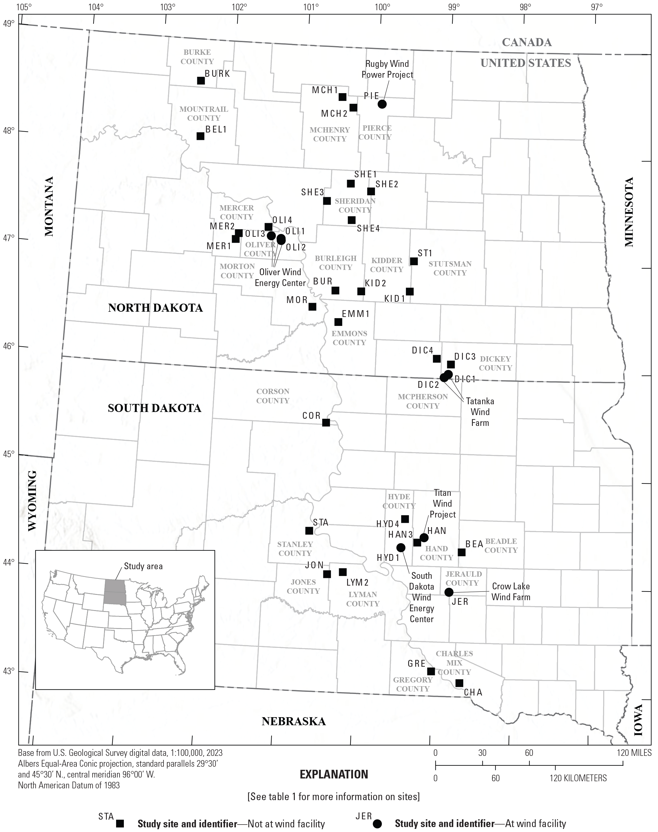
The location of study sites used to develop models for sharp-tailed grouse (Tympanuchus phasianellus) lek density and average number of males per lek in North Dakota and South Dakota, United States, 2000–14.
Table 1.
Information for study sites used to develop models for sharp-tailed grouse (Tympanuchus phasianellus) lek density in North Dakota and South Dakota, 2000–14.[SDDGFP, South Dakota Department of Game, Fish and Parks]
The overall goal was to assess the feasibility of using independently derived, long-term datasets gathered in North Dakota and South Dakota to determine whether wind facilities affected lek metrics. The specific objectives included the following:
-
1. Consolidate lek survey data from the USGS, North Dakota Game and Fish Department (NDGF), South Dakota Department of Game, Fish and Parks (SDDGFP), USFS, and WEST into a common data framework for further analyses.
-
2. Assess the strength and weaknesses of each of the datasets and provide a synopsis of this evaluation.
-
3. Assess the strength of association between a suite of explanatory variables and lek density and average number of males per lek.
-
4. Assess if the addition of a wind facility within the landscape explains variation in lek metrics beyond those explained in objective 3.
Study Area
The study area was defined by the coverage of data from lek routes surveyed by the USGS, NDGF, SDDGFP, USFS, and WEST. This coverage was largely contained within the Missouri Coteau region of North Dakota and South Dakota (fig. 1). The Missouri Coteau was our focus because it harbors grasslands that will become increasingly more important for sharp-tailed grouse as grasslands continue to disappear owing to conversion to cropland and other land uses (Lark and others, 2015, 2020). The lek survey routes traversed, on average, an approximately 9.656-km by 9.656-km area (93.238 square kilometers [km2], which equates to the size of a typical legal township). To establish study sites of equal area, we used ArcMap version 9.3 (Esri, Redlands, California) to visually select the center of each lek survey route. This center was considered to be the centroid of a 9.656- × 9.656-km block. This 93.238-km2 block (or study site) was considered the primary sampling unit or replicate for subsequent estimates and analyses.
Methods
Lek survey data were obtained from six sources: North Dakota lek surveys (North Dakota Game and Fish Department, 1963); USGS lek surveys; WEST, Inc., lek surveys (C. Derby, WEST, Inc., written commun., February 22, 2023); South Dakota lek surveys (South Dakota Department of Game, Fish and Parks, 2022); a South Dakota telemetry study (Runia and Solem, 2015); and the USFS Fort Pierre National Grassland (Schenbeck and Moravek, 1988). Information concerning these methods are included in this section.
Grouse Lek Surveys
Since 1963, the NDGF has run annual, standardized survey routes for sharp-tailed grouse (North Dakota Game and Fish Department, 1963). Lek counts determine an accurate count of males on previously identified and still-active leks, on leks that may have moved, and on newly established leks. Observers attempted to obtain three counts per lek where weather, travel conditions, and landowner access allowed. Lek counts occurred from early April through mid-May and from half an hour before sunrise until 1 to 2 hours after sunrise. Subsequent counts of the same lek varied as to time of day, as well as the day relative to peak breeding activity; that is, a before-sunrise and an after-sunrise count, as well as an early- and late-period count, were advised. Lek location was recorded using a Global Positioning System (GPS). The preferred lek count occurred from a vehicle, allowing for minimal disturbance to birds on leks. Where land access was granted and leks could not be adequately viewed from roads, observers conducted walk-in surveys. If the use of vehicles was not an option, observers approached leks on foot slowly, using topographical features to obscure presence. Birds sometimes flushed but normally returned shortly after disturbance abated, especially early in the mornings and during the peak lekking period. Counts continued as long as grouse were present. The time spent at each lek depended on bird activity and topography. If birds appeared to still be arriving, or if topography was such that individual birds were able to disappear and appear from view, observers were advised to stay at the observation point longer. Males were most easily identified when displaying, and counts were easier to obtain when the males on a lek were all or nearly all actively displaying than when activity was at a standstill. Leks often had one main dancing ground, but isolated males and small groups were observed to dance several yards to several hundred yards from the main display ground. Thus, care was taken to look for grouse in outlying areas. Depending on distance and number of males at these outlying areas, these areas were deemed as satellite leks and noted as such on the field form. Birds chased away by known males were counted as males; birds allowed to enter lekking grounds near known males were counted as females. If no eye comb was present, the bird never displayed, and the bird was ignored by a known male, that individual was counted as a female. In situations where a count from a vehicle was impossible, and a walk-in count was likely to have low success owing to location of the lek on a high knoll that allowed the birds to spot observers, a flush count was allowable. However, when birds were flushed, gender could not always be determined. Flush counts sometimes also were made after a scoping effort to verify the estimate and that all birds had actually been seen and counted. The flight behavior during a flush count can be informative in the verification-flush scenario: females were more likely to keep flying off, as they had no real affinity for a particular lek. Males were more likely to just fly a short distance because they returned to the lek. Late-morning flush counts, after dancing activity had diminished or ceased (about 1.5 hours after sunrise), increased the chances of male-only attendance. Flush counts were most accurate in late March and early April and again in late April and early May, as female attendance was lowest during these time periods. Later-morning flush counts were preferrable to later-period flush counts, as male attendance declined later in the lekking season (North Dakota Game and Fish Department, 1963). Some lek survey routes were run near two wind facilities: Acciona’s Tatanka Wind Farm, Dickey County, North Dakota, and McPherson County, South Dakota; and NextEra Energy’s Oliver Wind Energy Center, Oliver County, N. Dak. (fig. 1, table 1).
The focus of USGS field efforts was the documentation of sharp-tailed grouse lek locations near and within wind-facility footprints and counts of birds on individual leks. USGS surveys followed the NGDF protocol (North Dakota Game and Fish Department, 1963). Selected wind facilities were situated within expanses of native grassland and in landscapes characterized by morainic rolling plains interspersed with wetlands; mixed-grass prairie pastures; and few planted grasslands, hayfields, or cropland. Five wind facilities (fig. 1, table 1) met these criteria: Acciona’s Tatanka Wind Farm; Avangrid Iberdrola Renewables’ Rugby Wind Power Project, Rugby, Pierce and Rolette Counties, N. Dak.; Clipper Windpower and BP Alternative Energy’s Titan Wind Project, Hand County, S. Dak.; NextEra Energy’s Oliver Wind Energy Center; and NextEra Energy’s South Dakota Wind Energy Center, Hyde County, S. Dak.
WEST surveyed leks within the Avangrid Iberdrola Renewables’ Rugby Wind Power Project (fig. 1, table 1). The protocol generally followed the NDGF protocol (North Dakota Game and Fish Department, 1963). Public roads within the boundary of the facility were driven half an hour before sunrise to 2 hours after sunrise. Observers stopped every 0.80 km for at least 5 minutes to listen and look for displaying grouse. When a lek was observed, the time, temperature, lek location, distance from road, direction of road, number of males, number of females, and number of unknown-gender birds were recorded (C. Derby, WEST, Inc., written commun., February 22, 2023).
From the early 1950s through 2019, SDDGFP staff annually searched previously established survey areas measuring 104 km2 for leks and counted all males attending leks (South Dakota Department of Game, Fish and Parks, 2022). Routes contained a road or trail to provide vehicular access (South Dakota Department of Game, Fish and Parks, 2012). Surveys were run from late March to late April. Active leks from previous years were checked for current-year activity by a site visit. Counts of leks consisted of early morning surveys in which the total number of grouse, reported as number of males and number of females, was recorded. Repeat counts of males were conducted until the observer was satisfied of an accurate count. New leks were discovered by running early-morning listening surveys during which observers listened for previously undetected grounds and triangulated until the location of the new lek was determined. During listening runs, stops were made at intervals of no more than 1.6 km (1 mile) apart. Numbers of male and female grouse were recorded for all leks. All discovered leks were identified with GPS coordinates (South Dakota Department of Game, Fish and Parks, 2012). One survey area encompassed the Crow Lake Wind Farm, Jerauld Co. S. Dak, beginning in 2011 (fig. 1, table 1).
From 2010 to 2013, SDDGFP piloted a telemetry study of sharp-tailed grouse in Hand and Hyde Counties to determine female survival and fecundity (Runia and Solem, 2015). Staff collected lek-count data within the 93.238-km2 study site as part of this research effort and followed a survey design that was structured similarly to the State’s annual grouse surveys (South Dakota Department of Game, Fish and Parks, 2012). Lek activity was monitored from mid-March through April from 2010 to 2012, with searches commencing half an hour before sunrise to 2 hours after sunrise, and 1 hour before sunset to half an hour after sunset. The number of male grouse were counted 1–3 times. All leks were marked with a GPS.
Since 1988, the U.S. Forest Service has run lek surveys on the 7,386-hectare Cedar Creek Monitoring Unit of the Fort Pierre National Grassland in South Dakota (Schenbeck and Moravek, 1988). The goal of the survey was to count males at least once, but preferably, three times. The survey period ran from early April to mid-May. Surveys were conducted from half an hour before sunrise until 2 hours after sunrise. Surveys occurred on drivable roads, with stops at 1.6-km intervals to listen for displaying male grouse. Observers stayed within vehicles for the survey. Where a lek was observed, the observer attempted to drive within 91.4 meters of the lek to obtain an accurate male count.
Response Variables
Sharp-tailed grouse lek density and average number of males per lek were computed from lek survey data. Lek density (leks per square kilometer) was computed for each study site each year as the number of leks observed along the survey route for that study site divided by the area (square kilometers) covered by the survey that year; this number was then used as an estimate of lek density for the 93.238-km2 study site. An observation of one or more grouse together was considered a lek. The average number of males per lek was computed for each study site each year by first computing the maximum number of males counted for each lek and then averaging these values across leks within a study site per year. For individual grouse of unknown sex within a lek, the sex ratio (that is, proportion of males) for the study site-and-year combination was used to classify the unknown individual as male or female before computing the maximum number of males for each lek.
Explanatory Variables
We developed a suite of 24 biologically supported candidate variables associated with estimated lek metrics (table 2), including number of turbines, easting and northing coordinates, elevation, land cover, Palmer Drought Severity Index, and climate. These variables are described in this section.
The number of wind turbines within study site was determined by a simple count. The relation between sharp-tailed grouse lek metrics and spatial location was determined by reprojecting the latitude and longitude coordinates for each study site to Albers Equal-Area Conic Projection (in meters, but converted to kilometers for models). In general, sharp-tailed grouse densities tend to increase following a southeast-to-northwest gradient across North Dakota and South Dakota (Sauer and others, 2013). Topography may affect the detection of birds (Dawson, 1981), densities of birds (Renfrew and Ribic, 2002), and locations of leks (Hovick and others, 2015). Elevation data were downloaded from the USGS National Elevation Dataset (U.S. Geological Survey, 2005) for North Dakota and South Dakota. Elevation values (in meters) were extracted from each study site using ArcMap version 9.3 (Esri, Redlands, California). The mean and standard deviation for each study site were used to describe the topography and topographic roughness of the landscape.
Land-cover data were obtained from National Agricultural Statistical Service (NASS), and land-cover classes were extracted for each study site (U.S. Department of Agriculture, 2011). For each year, NASS data were used from the previous growing season. Land-cover values were collapsed into nine explanatory landscape variables (table 2). Given the changes in crop production in this region during the past decade, several crop classifications (as opposed to merging all crop classes) were maintained. In recent decades, agricultural production has shifted from small grains to corn (Zea mays) and soybeans (Glycine max) (Wright and Wimberly, 2013; Wimberly and others, 2017). Within each study site, the percentage cover for the 9 landscape variables was computed. NASS data were available for North Dakota for all years (1999–2013) of interest for this study, whereas NASS data for South Dakota were available for 2006–13. Thus, land cover was able to be associated with lek metrics only for these latter years in South Dakota.
Values from the Palmer Drought Severity Index (PDSI) were used as a measure of regional precipitation levels and moisture levels (Palmer, 1965; National Oceanic and Atmospheric Administration, 2023). The PDSI incorporates information on soil moisture and temperature to provide a monthly index of the severity of a wet (positive values) or dry (negative values) period by incorporating past and present conditions. Specifically, PDSI index values of 0 to −0.5 indicate normal moisture conditions; −0.5 to −1.0, incipient drought; −1.0 to −2.0, mild drought; −2.0 to −3.0, moderate drought; −3.0 to −4.0, severe drought; and less than (<) −4.0, extreme drought. Similar terms are associated with positive values and wet spells. PDSI data were extracted for each study site, and mean PDSI values from the previous 12 months of grouse surveys (prior April to March of current year of lek surveys) were computed to get a yearly mean. The mean values for the prior 4 months of spring (prior April through prior July) also were computed to represent the conditions from the prior spring’s nesting and early brood rearing periods (table 2), when nests and grouse are most vulnerable to weather conditions.
Precipitation and temperature data were obtained for each study site from 1999 to 2014 from the Parameter-elevation Regressions on Independent Slopes Model (PRISM) climate mapping database, which uses weather station data to model precipitation and temperature across space (Daly and others, 2008; Oregon State University, 2014). PRISM data contain spatially gridded values at the 4-km grid-cell resolution. Within each study site, four metrics from PRISM data were computed, including mean precipitation and mean, minimum, and maximum temperatures for two time periods: the prior 12 months (April–March) from the current year lek surveys and the prior spring 4 months representing prior spring breeding and brood rearing conditions (April–July; table 2).
Table 2.
Explanatory variables used to develop models for sharp-tailed grouse (Tympanuchus phasianellus) lek density and average number of males per lek in North Dakota and South Dakota, United States, 2000–14.[STGR, sharp-tailed grouse; NASS, National Agricultural Statistical Service; PDSI, Palmer Drought Severity Index; cm, centimeter; °C, degree Celsius; TMAX, average maximum temperature]
| Explanatory variable | Variable definition | Justification |
|---|---|---|
| NUMTURB3 | Number of turbines within study site | Female greater prairie-chickens (Tympanuchus cupido) (GRPC) avoided wind turbines (Winder and others, 2014). STGR nest-site selection and daily nest survival (Proett and others, 2019) were not affected by number of turbines. |
| XALBERS | Estimated Easting center of each study site, in kilometers | Abundance of some species of grassland birds and waterfowl varied with longitude (Reynolds and others, 1994; O’Connor and others, 1999). |
| YALBERS | Estimated Northing center of each study site, in kilometers | Grouse (Tympanuchus and Bonasa species) exhibited latitudinal patterns of population dynamics (Williams and others, 2004). Ring-necked pheasant (Phasianus colchicus) (RNEP) abundance increased with latitude (O’Connor and others, 1999). |
| MEAN_Z | Mean elevation of sample points within study site, in meters | STGR were most likely to use elevations higher than 900 meters during the nonbreeding season (Hiller and others, 2019). GRPC were more likely to select higher elevations (relative to the surrounding landscape) for lek sites (Gregory and others, 2011). |
| STD_Z | Standard deviation of sample points of elevation within study site, in meters | Male STGR and greater sage-grouse (Centrocercus urophasianus) (GRSG) used less rugged areas more intensely within the spring-to-summer home ranges (Stonehouse and others, 2015). Elevation was an important predictor of lek location for GRPC (Hovick and others, 2015). Topography can affect density of grassland birds (Renfrew and Ribic 2002). |
| NASSP1 | Percent of landscape classified as water (NASS classes 83, 87, 111, 190, 195) for the previous growing season | GRPC distribution probabilities during breeding season were near wet meadows and were positively influenced by peripheries of wetlands during nonbreeding season, whereas STGR distribution probabilities during both seasons were more distant from wet meadows (Hiller and others, 2019). |
| NASSP2 | Percent of landscape classified as cropland planted to corn (Zea mays) (NASS classes 1, 12, 13) for the previous growing season | RNEP abundance was positively associated with corn (O’Connor and others, 1999). |
| NASSP3 | Percent of landscape classified as cropland planted to pulse crops and soybeans (Glycine max) (NASS classes 5, 42, 52, 53, 241) for the previous growing season | Abundances of some species of grassland birds were positively associated with soybeans (O’Connor and others, 1999). |
| NASSP4 | Percent of landscape classified as cropland planted to wheat (Triticum species) and other small grains (NASS classes 21–29, 205, 225, 236, 240) for the previous growing season | RNEP and other grassland species abundances were positively associated with small grains (O’Connor and others, 1999). |
| NASSP5 | Percent of landscape classified as cropland planted to oil seeds and miscellaneous crops (NASS classes 4, 6, 31–35, 38, 39, 41, 43, 44, 47, 57, 61, 65, 246) for the previous growing season | Abundances of some species of grassland birds were positively associated with oil-seed cropland (O’Connor and others, 1999). |
| NASSP6 | Percent of landscape classified as hayland (NASS classes 36, 37, 58, 60) for the previous growing season | STGR and GRPC occurrence and density were positively associated with grass (Runia and others, 2021). Abundance of GRPC was positively associated with hayland (O’Connor and others, 1999). |
| NASSP7 | Percent of landscape classified as pasture (NASS classes of 59, 62, 171, 176, 181, 182) for the previous growing season | STGR and GRPC occurrence and density were positively associated with grass (Runia and others, 2021). GRPC lek presence was positively associated with pasture (Runia, 2009). |
| NASSP8 | Percent of landscape classified as shrub-forest (NASS classes of 63, 141–143, 152) for the previous growing season | STGR abundance decreased 74.5 percent with tree cover and 15.1 percent over low-to-high values of shrubby-grassland cover (Stevens and others, 2023). |
| NASSP9 | Percent of landscape classified as low, medium, and high intensity developed classes | STGR and GRPC occurrence and density were negatively associated with developed areas (Runia and others, 2021). Effect of energy infrastructure, roads, and other developments on GRPC, lesser prairie-chickens (Tympanuchus pallidicinctus), and GRSG summarized in Rowland (2019), Jamison and others (2020), Svedarsky and others (2022). |
| PDSI_1 | Mean PDSI from prior April through March current year of lek surveys (12 months) | GRPC nest survival was not affected by PDSI (Harrison and others, 2017). |
| PDSI_3 | Mean PDSI from prior April through prior July from current year of lek surveys (4 months) | GRPC abundance was highest following wetter summers, cooler summers, drier winters, and cooler winters (Schindler and others, 2020). |
| PPT_X1 | Mean precipitation (cm) from prior April through March current year of lek surveys (12 months) | STGR probability of presence was highest in areas with mean precipitation greater than 11.3 cm, and GRPC occurrence and density had a quadratic response to long‐term (1981–2010) mean annual precipitation (Runia and others, 2021). Larger prairie grouse (Tympanuchus spp.) juvenile:adult ratios in the fall (indicative of higher rates of chick survival) were positively associated with cumulative precipitation measured from January to July (Flanders-Wanner and others, 2004). |
| PPT_X3 | Mean precipitation (cm) from prior April through prior July from current year of lek surveys (4 months) | STGR abundance increased 75.5 percent from low to high values of early spring precipitation, measured the prior year (Stevens and others, 2023). STGR probability of presence was highest in areas with mean precipitation greater than 11.3 cm in spring (Hiller and others, 2019). |
| TMEAN_X1 | Average mean temperature (°C) from prior April through March current year of lek surveys (12 months) | STGR ranked low in vulnerability to increases in temperature during the breeding season (Wilsey and others, 2019). |
| TMEAN_X3 | Average mean temperature (°C) from prior April through prior July from current year of lek surveys (4 months) | STGR abundance and productivity were not associated with late spring temperature (Stevens and others, 2023). |
| TMIN_X1 | Average minimum temperature (°C) from prior April through March current year of lek surveys (12 months) | STGR occurrence and density were negatively associated with the long‐term (1981–2010) minimum January temperature (Runia and others, 2021). |
| TMIN_X3 | Average minimum temperature (°C) from prior April through prior July from current year of lek surveys (4 months) | STGR abundance or productivity were not associated with late spring temperature (Stevens and others, 2023). |
| TMAX_X1 | Average maximum temperature (°C) from prior April through March current year of lek surveys (12 months) | GRPC abundance was highest in years following low summer TMAX (Schindler and others, 2020). |
| TMAX_X3 | Average maximum temperature (°C) from prior April through prior July from current year of lek surveys (4 months) | STGR abundance or productivity were not associated with late spring temperature (Stevens and others, 2023). |
Data Analysis
Trends in lek density and mean number of males per lek during the 15 years (2000–2014) of the study were examined by computing yearly mean estimates. These estimates were computed using a repeated measures model (Stroup, 2013) for each response variable (that is, lek density or number of males per lek). The response variables were assumed to follow a normal distribution. Year, State, and interaction between State and year were included in the model as fixed factors, so that yearly estimates could be computed separately for each State and averaged across States. Study site-within-State was included as a random effect to account for the repeated measures on each study site. An autoregressive covariance structure was assumed to account for the correlation among years (Stroup and others, 2018). Least squares mean estimates of yearly lek density and number of males per lek for each State were computed and summary plots created. Overall averages by year (States averaged) and State (years averaged) also were computed. To prevent study sites that were only surveyed a few years from having too much effect on the variability in estimates from year to year, the square root of the number of years for each study site was used as a weight; therefore, the estimated State-by-year least squares means are weighted averages.
Twenty-four geographic, landscape, and climate variables were measured and included in analyses as the potential explanatory variables (table 2). The association between explanatory variables and the response variables was assessed using information theoretic methods (Burnham and Anderson, 2002). Linear mixed models were fit for each response variable. The response variables were assumed to follow a normal distribution. The explanatory variables were included in the models as fixed effects, and study site was included as a random effect to account for the repeated measures on each study site. An autoregressive covariance structure was assumed to account for the correlation among years (Stroup and others, 2018). To prevent study sites that were only surveyed a few years from having too much influence on the estimates, the square root of the number of years for each study site was used as a weight. The candidate set of models consisted of all one- and two-variable models along with the null model. However, if the two variables in a two-variable model had a correlation of greater than or equal to 0.7 or less than or equal to −0.7 (tables 1.1, 1.2, 1.3), then that model was removed from the candidate set. For each response variable, Akaike’s Information Criterion for small samples (AICC), delta AICC, and Akaike weight were computed for each model in the candidate set (Burnham and Anderson, 2002). Delta AICC was computed for a model as the AICC for that model minus AICC from model with the lowest AICC value.
Nine study sites had wind turbines during the later years of the study. Estimates of average lek density and average number of males per lek were computed by year for study sites with turbines present and for study sites without turbines. These estimates were computed using a repeated measures model (Stroup, 2013) for each response variable. The response variables were assumed to follow a normal distribution. A means model approach was used, and the interaction between year and turbine presence was included in the model as a fixed factor, so that yearly estimates could be computed separately for turbine and nonturbine study sites. Study site was included as a random effect to account for the repeated measures on each study site. An autoregressive covariance structure was assumed to account for the correlation among years (Stroup and others, 2018). To prevent study sites that were only surveyed a few years from having too much influence on the variability in estimates from year to year, the square root of the number of years for each study site was used as a weight. Models were run separately for each State. For each State, only years in which turbines were present and sharp-tailed grouse were observed in the turbine sites were included in the analyses (that is, 2008–14 for North Dakota and 2010–14 for South Dakota). All models were run using the mixed linear models procedure in SAS statistical software (SAS Institute Inc., 2020).
Results
Data were collected and analyzed from 37 study sites covering the years 2000–14. Sharp-tailed grouse leks were present in nearly all study sites every year. Lek density and mean number of males per lek were estimated.
Grouse Lek Surveys
Of the 37 study sites, 25 study sites were in North Dakota and 12 were in South Dakota (fig. 1, table 1). Each study site was surveyed from 2 to 15 years: 30 percent were surveyed 15 years, 24 percent were surveyed 10–14 years, and 14 percent were surveyed <5 years.
Assessment of the Data
Survey routes for sharp-tailed grouse appear to have been historically established in areas in which leks were known to occur, as opposed to establishing survey routes using a random process. Therefore, our estimates of lek density reflect an average lek density for locations where grouse were present. Formal protocols for gathering survey data indicate that an area of a known size is to be surveyed. However, for all study sites included in the study, there is no indication whether observers faithfully surveyed the entire area each year, or if they just surveyed previously known leks. It is further not indicated for what years this may have happened. Because lek density was computed by dividing the number of leks observed by the area (square kilometers) covered by the survey route (but whether that area was faithfully surveyed every year is unknown), the accuracy of the observed lek density estimates is unknown.
The datasets contained numerous instances in which individuals were recorded, but a sex was not assigned to the bird. To account for this in the analyses, the observed sex ratio (for the birds in which the sex was identified) was used to classify the unknown individuals as male or female. This technique introduced error (that is, bias) into the estimates of the number of males per lek, but the extent of this error is unknown.
Very few turbine study sites were included in this study and those that did occur were clustered into several locations, but control sites were more evenly spaced within the study area (fig. 1). The uneven distribution of turbine and control sites made it difficult to assess the effects of turbine facilities; any differences observed between turbine and nonturbine study sites could be due solely to location differences.
Lek Density and Mean Number of Males Per Lek
Number of sharp-tailed grouse leks observed during surveys ranged from 0 to 35. Leks were observed during almost every survey; <2 percent of the surveys included in this study observed zero sharp-tailed grouse leks. Lek density ranged from 0 to 0.38 lek per square kilometer with a mean of 0.10 (standard error=0.004). Average number of males observed per lek ranged from 1 to 34 with a mean of 12 (standard error=0.3). Summary statistics for both response variables and the explanatory variables are given in table 3.
Table 3.
Summary statistics for response and explanatory variables used to develop models for sharp-tailed grouse (Tympanuchus phasianellus) lek density and average number of males per lek in North Dakota and South Dakota, 2000–14.[n, number year-by-study site combinations for all variables except xalbers, yalbers, mean_z, and std_z, where n is the number of study sites; SD, standard deviation; Min, minimum; Max, maximum; LEKDENS_SQKM, lek density per square kilometer; MEAN_XMALES1_LEK, mean number of males per lek; km, kilometer; m, meter; NASS, National Agricultural Statistical Service; %, percent; PDSI, Palmer Drought Severity Index; cm, centimeter; °C, degree Celsius]
With the exception of LEKDENS_SQKM and MEAN_XMALES1_LEK, all variables defined in table 2.
Mean lek density and mean number of males per lek were estimated for each State each year (table 4). Weighting was done by square root of number of years for each study site. An overall average for each year (computed as an average of the two State values for that year) and for each State (computed as an average of the year values for that State) were also computed. Mean lek density estimates in North Dakota were 1.4–3.4 times those in South Dakota (table 4, fig. 2). There was less of a difference for mean number of males per lek, but North Dakota estimates were still 1.2–3.1 times those in South Dakota (table 4, fig. 3). For both response variables, the estimates varied across years.
Table 4.
Yearly least squares means (standard error) for lek density and mean number of males per lek by State and averaged across States for models developed for sharp-tailed grouse (Tympanuchus phasianellus) in North Dakota and South Dakota, 2000–14.[n, number of observations; weighting was done by square root of number of years for each study site]
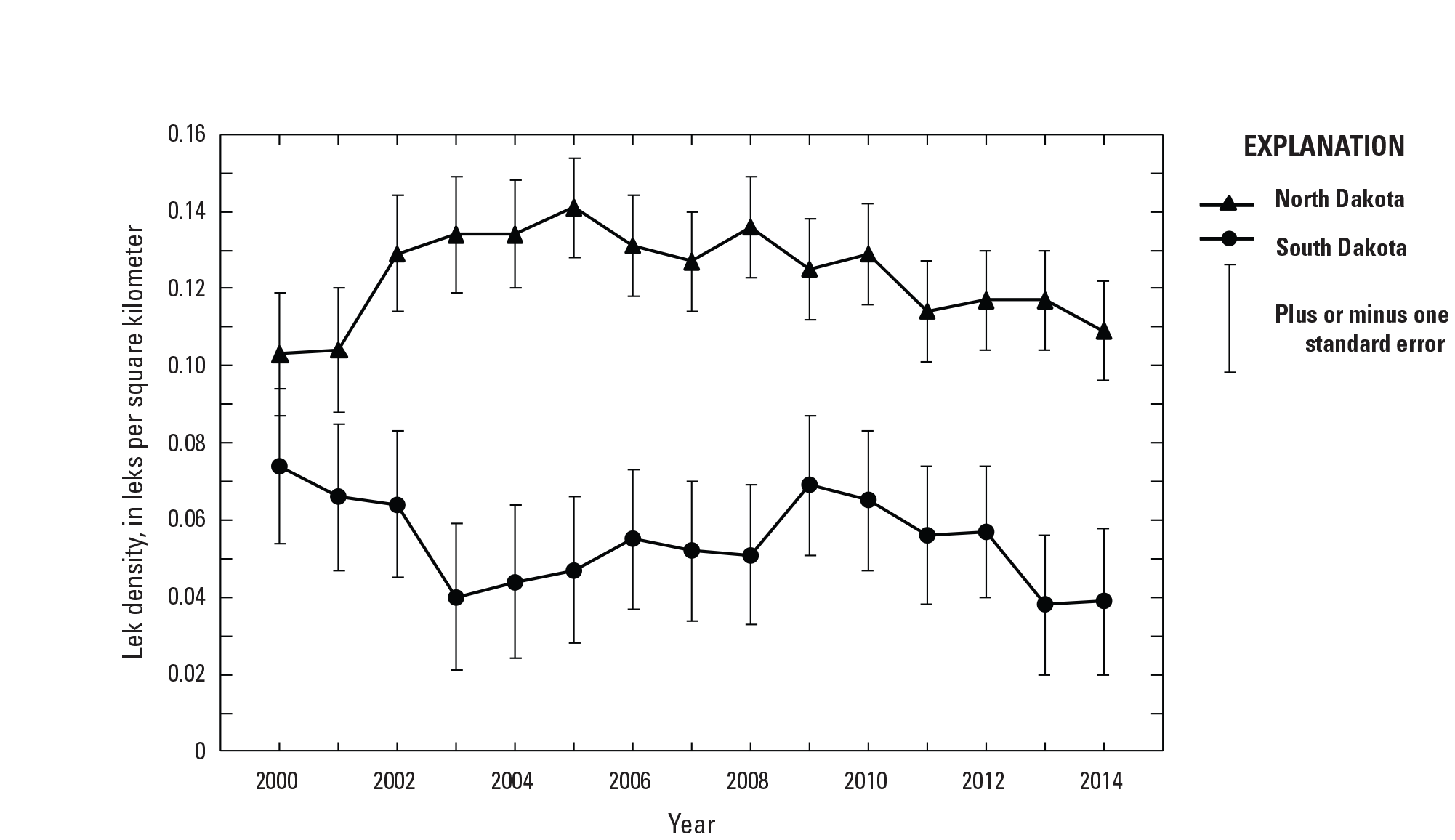
Sharp-tailed grouse (Tympanuchus phasianellus) mean lek density by year for North Dakota and South Dakota, 2000–14.
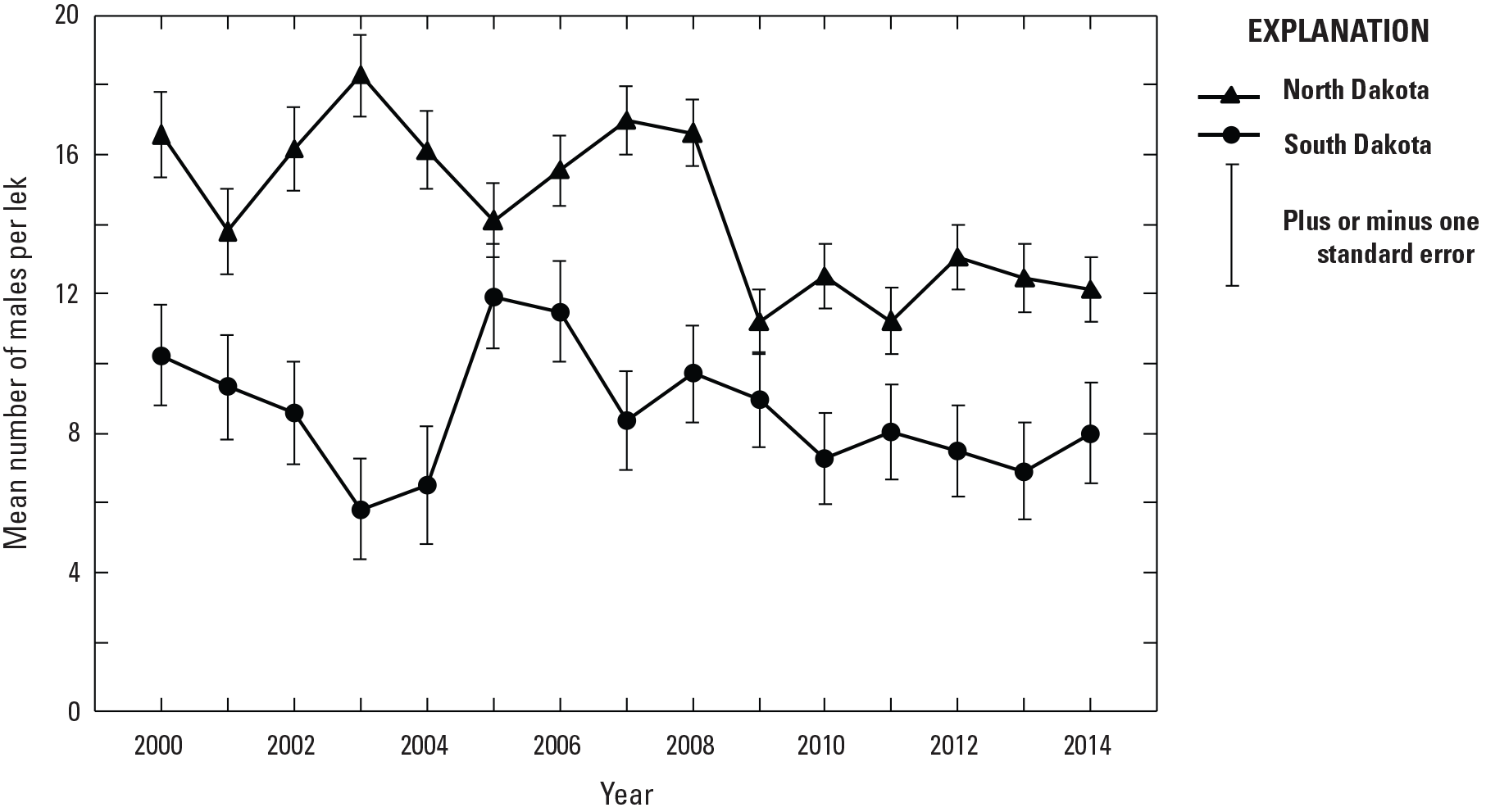
Mean number of sharp-tailed grouse (Tympanuchus phasianellus) males per lek by year for North Dakota and South Dakota, 2000–14.
Of the 24 explanatory variables, Northing (YALBERS) was most important for predicting lek density across North Dakota and South Dakota (table 5). Out of 20 models with a difference of AICC for model minus AICC for model with the lowest AICC value (ΔAICC) <4, 13 contained Northing, including the model with Northing alone, which was the best one-variable model. Easting (XALBERS) was the next most common variable and was in 8 of the top 20 models. No other variable occurred more than twice (once with Northing and once with Easting). Northing had a positive association with lek density (fig. 4), and Easting had a negative association. However, even the “best” model (model with lowest AICC) only had an Akaike model weight of 0.09, and plots of observed versus predicted values for this model revealed a poor model fit. It is not surprising that Northing was most associated with lek density given the results of the previous analysis. Therefore, to determine what variables are most associated with lek density other than the State difference, analyses were rerun separately by State. For North Dakota, NASSP4 (a variable representing percentage of small grains) (fig. 5) and PPT_X1 (a variable representing 12-month precipitation) were most associated with lek density. Both variables were in the top model that had a model weight of 0.17, and both variables were negatively associated with lek density. NASSP4 was in 4 of the 6 models with ΔAICC<4, and PPT_X1 was in 2 of the models. NASSP6 (a variable representing percentage hayland) was also in 2 of the 6 models with ΔAICC<4. For South Dakota, there were 9 models with a ΔAICC<2 and 57 models with ΔAICC<4. NASSP8 (a variable representing percentage shrub/forest) (positive association, fig. 6) was the most common variable in the 9 models with ΔAICC<2. However, for both North Dakota and South Dakota, plots of observed versus predicted values for the top models indicated that none of these variables were good at predicting lek density. Therefore, there was little association between the explanatory variables examined in this report and lek density within this study.
Table 5.
Information theoretic results for models for sharp-tailed grouse (Tympanuchus phasianellus) lek density in North Dakota and South Dakota, 2000–14.[n, number of observations; k, number of parameters; LL, log likelihood; AICC, Akaike information criteria; ΔAICC, difference of AICC for model minus AICC for model with the lowest AICC value; w, Akaike weight; NASS, National Agricultural Statistical Service; PDSI, Palmer Drought Severity Index; candidate set included all 1 and 2 variable models except 2 variable models where 2 variables have a correlation of greater than or equal to 0.7 or less than or equal to −0.7. Models with ΔAICC less than 2 are reported]
All variables defined in table 2.
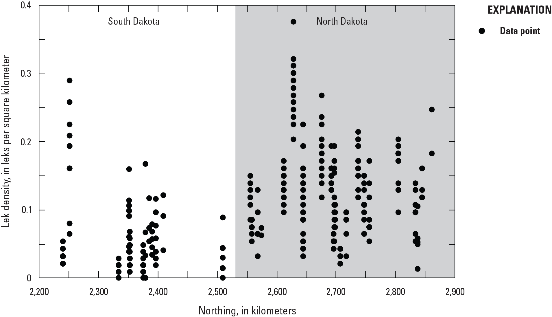
Sharp-tailed grouse (Tympanuchus phasianellus) lek density by northing (in kilometers) for North Dakota and South Dakota, 2000–14.
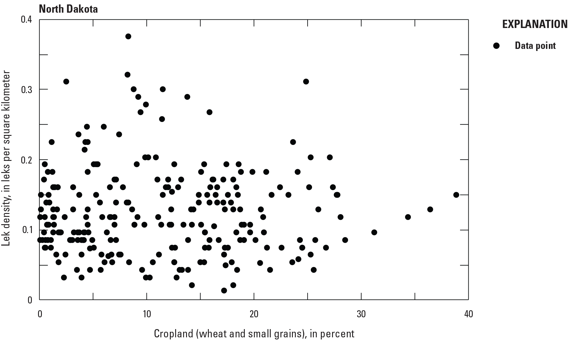
Sharp-tailed grouse (Tympanuchus phasianellus) lek density by percentage of landscape classified by the National Agricultural Statistical Service as cropland planted to wheat (Triticum species) and other small grains (NASSP4) for the previous growing season, North Dakota, 2000–14.
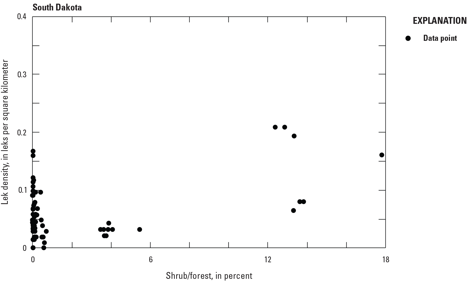
Sharp-tailed grouse (Tympanuchus phasianellus) lek density by percentage of landscape classified by the National Agricultural Statistical Service as shrubs or forest (NASSP8) for the previous growing season, South Dakota, 2000–14.
For mean number of males per lek in North Dakota and South Dakota, the top model contained Northing and TMIN_X1 (a variable representing 12-month minimum temperature) (table 6). Both Northing (fig. 7) and TMIN_X1 were positively associated with mean number of males per lek. The second-best model had a ΔAICC=7.09 and also contained Northing; the 24 models in the candidate set containing Northing were the top 24 models followed by the 23 models containing TMIN_X1. The model weight for the top model was 0.96, indicating it was by far the best model in the candidate set for predicting mean number males per lek. However, plots of observed versus predicted values still indicated that it was a poor predictive model. Similar to the analysis for lek density, the analysis for mean number of males per lek was rerun by State to remove the apparent State effect and to determine which variables were most associated with mean number males per lek for each State. For North Dakota, the top model contained precipitation variables PPT_X1 and PPT_X3 (a variable representing 4-month precipitation); this model had an Akaike weight of 0.86. PPT_X1 was negatively associated with mean number males per lek (fig. 8), whereas PPT_X3 was positively associated with number of males per lek. The second-best model had a ΔAICC=6.35. Similar to the model for both States, the best model for North Dakota was definitely better than the rest of the models in the candidate set but still was not a good predictive model. For South Dakota, there were 15 models with ΔAICC<2; NASSP8 (fig. 9) was in 10 of these and NASSP6 was in 5 of these. Similar to lek density, there seems to be little association between the explanatory variables examined in this report and the mean number of males per lek within this study.
Table 6.
Information theoretic results for models of mean number of males per lek for sharp-tailed grouse (Tympanuchus phasianellus) in North Dakota and South Dakota, 2000–14.[n, number of observations; k, number of parameters; LL, log likelihood; AICC, Akaike information criteria; ΔAICC, difference of AICC for model minus AICC for model with the lowest AICC value; w, Akaike weight; for variable definitions in Models see table 2; NASS, National Agricultural Statistical Service; candidate set included all one- and two-variable models except two-variable models where two variables have a correlation of greater than or equal to 0.7 or less than or equal to −0.7. Models with ΔAICC less than (<) 2 are reported here (however, only models with ΔAICC<1 were reported for South Dakota owing to the excess number of models with ΔAICC<2)]
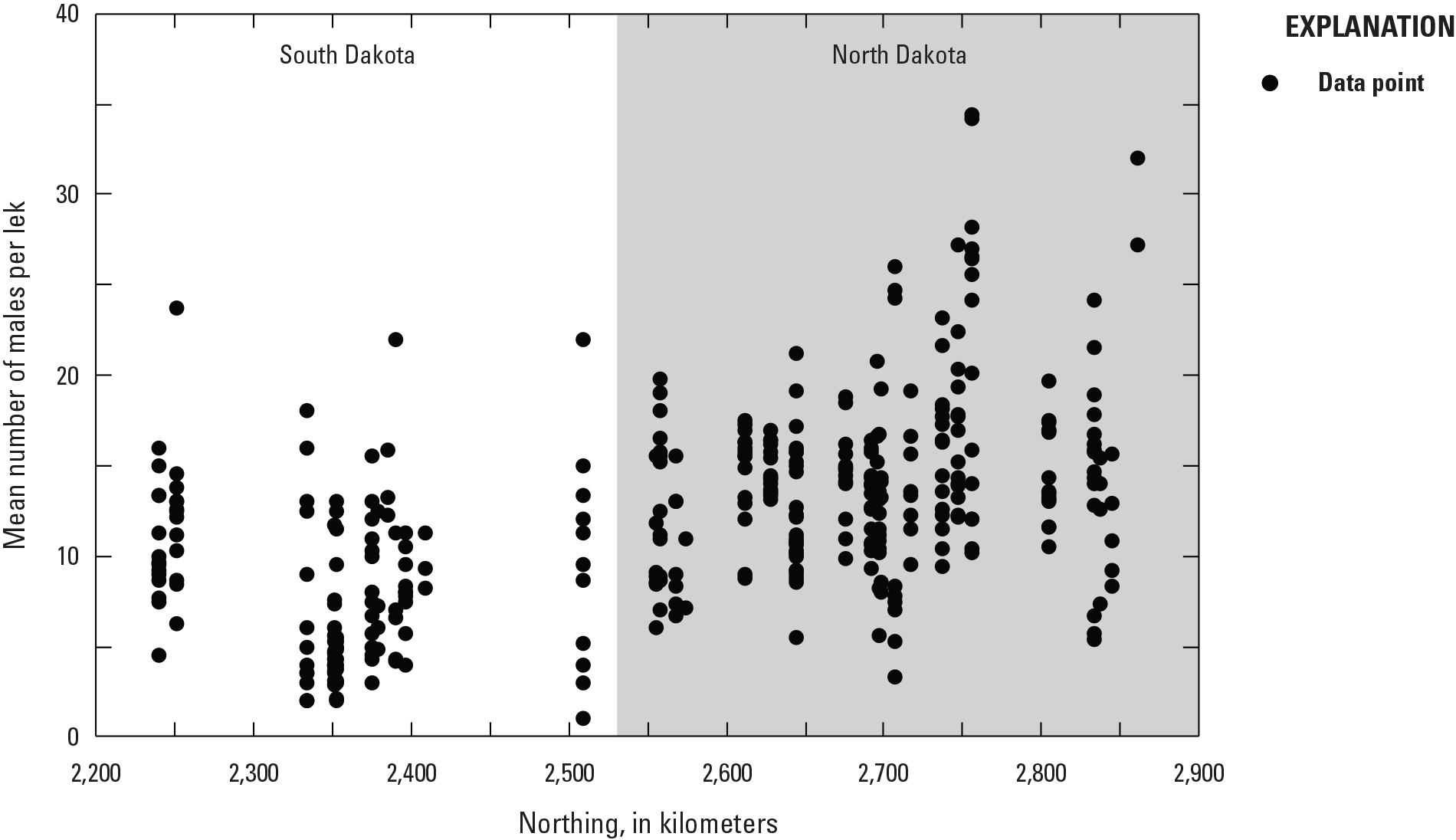
Mean number of sharp-tailed grouse (Tympanuchus phasianellus) males per lek by northing (in kilometers) for North Dakota and South Dakota, 2000–14.
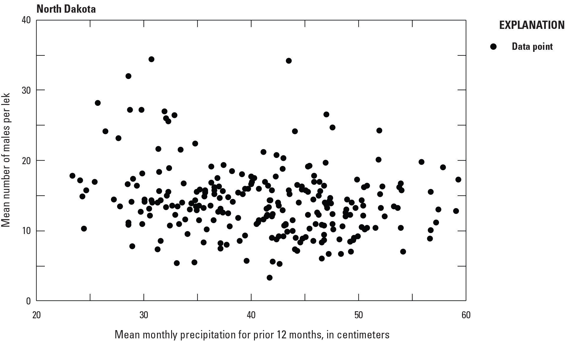
Mean number of sharp-tailed grouse (Tympanuchus phasianellus) males per lek by mean monthly precipitation for the prior 12 months (PPT_X1), North Dakota, 2000–14.
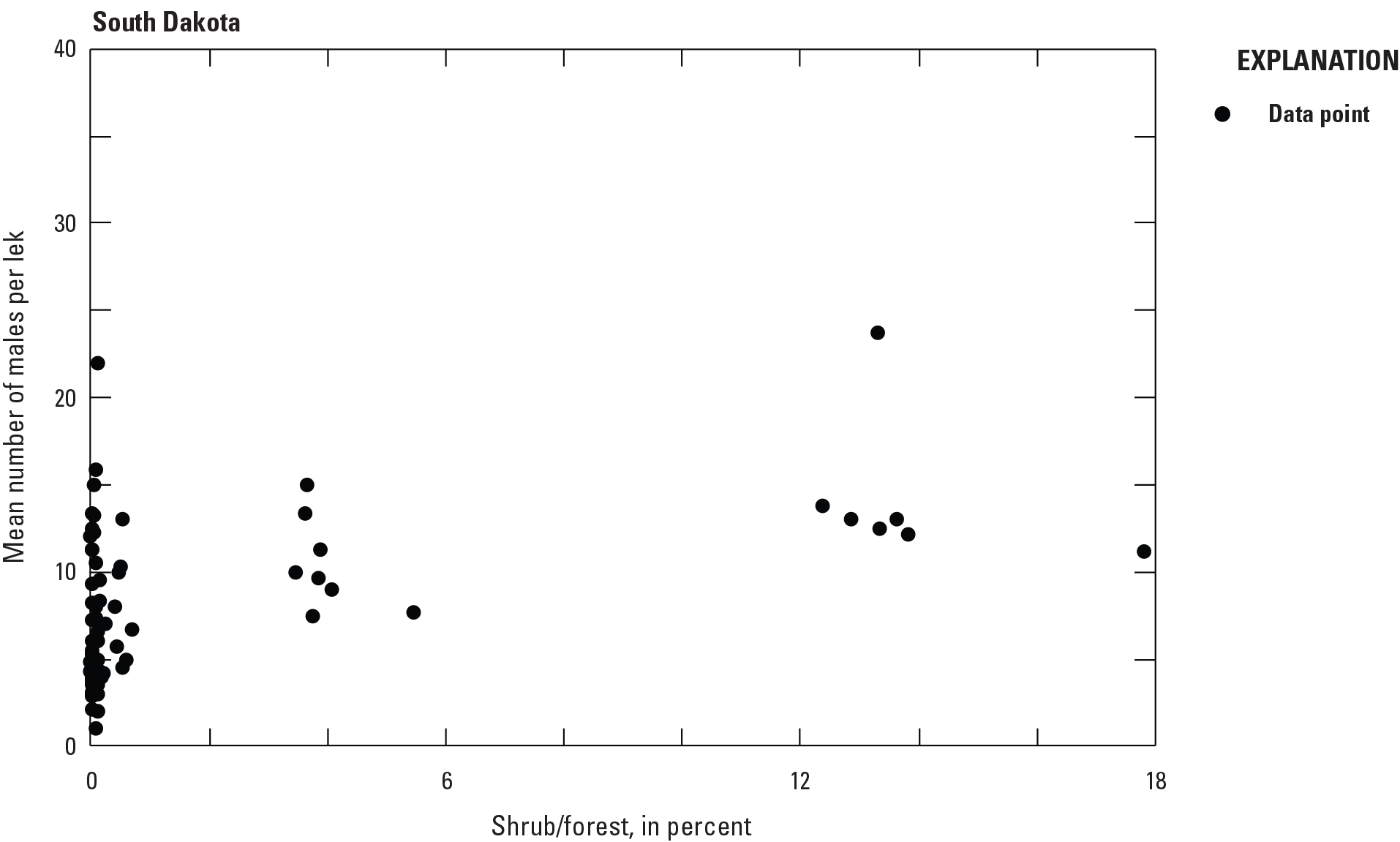
Mean number of sharp-tailed grouse (Tympanuchus phasianellus) males per lek by percentage of landscape classified by the National Agricultural Statistical Service as shrubs or forest (NASSP8) for the previous growing season, South Dakota, 2000–14.
Of the 37 study sites, 9 had turbines for part of the timeframe of this study (table 7, figs. 10–11). The number of turbines per site ranged from 1 to 83. The first year with turbines was 2005 (table 7). Mean lek density and mean number of males per lek were estimated for turbine and nonturbine study sites for each year turbines were present within North Dakota (table 8) and South Dakota (table 9). Mean lek density in nonturbine study sites in North Dakota was 1.1–1.2 times the estimates for turbine study sites, except for 2014 where the nonturbine site estimate was 1.5 times that in turbine sites. In South Dakota, the results varied with year; estimated mean lek density was higher in nonturbine sites in some years and higher in turbine sites in other years. Results were similar for mean number of males per lek, with estimates in nonturbine sites 1.0–1.2 times those in turbine sites in North Dakota. In South Dakota, the differences were greater, with estimates in nonturbine sites 1.0–1.9 times those in turbine sites. Differences, however, were not statistically compared owing to the unbalanced distribution of turbine and nonturbine sites.
Table 7.
Number of turbines per year in North Dakota and South Dakota, used to develop models for sharp-tailed grouse (Tympanuchus phasianellus) lek density and average number of males per lek, 2000–14.Study site acronyms are identified in table 1.
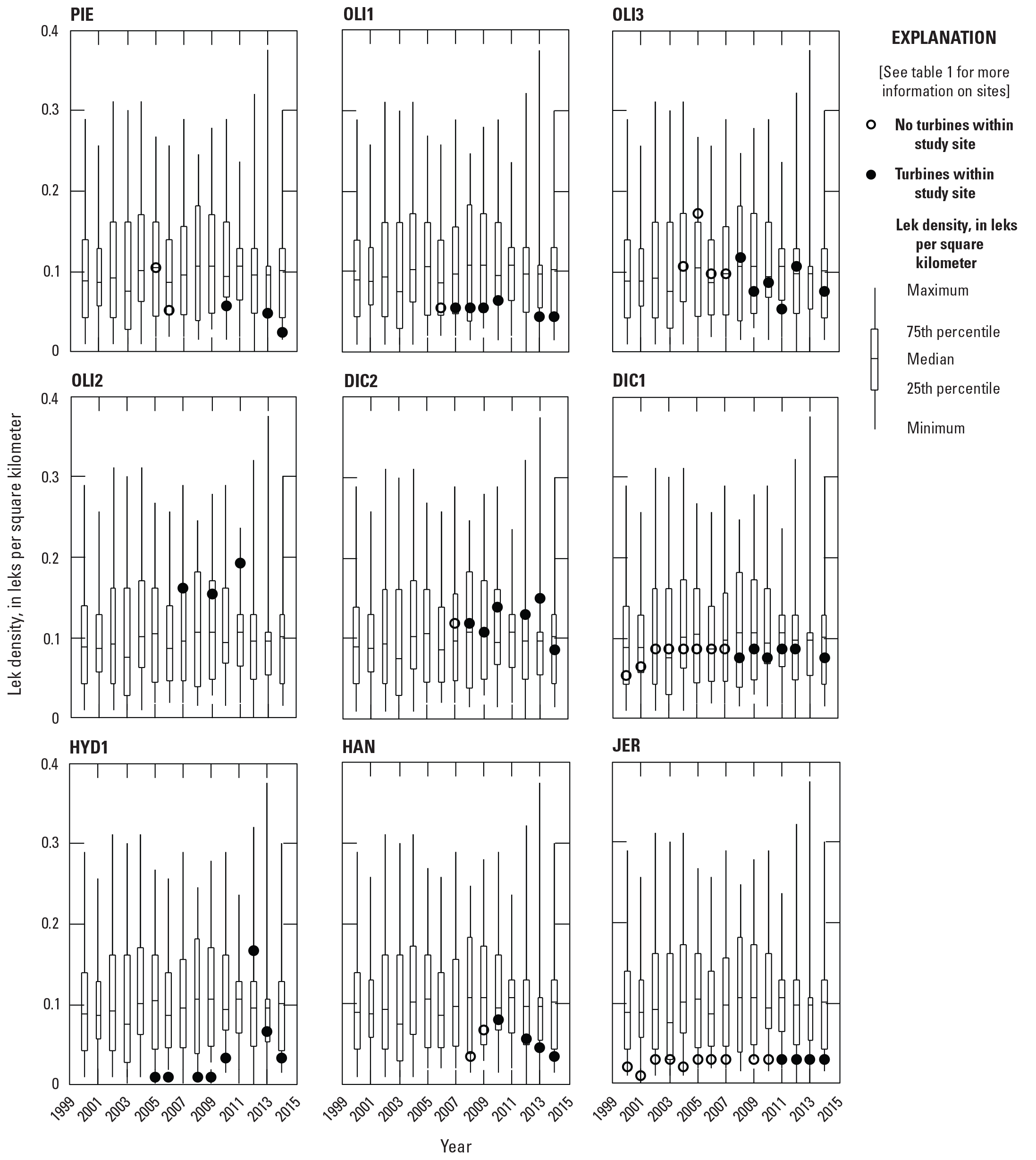
Sharp-tailed grouse (Tympanuchus phasianellus) lek density for each of the nine study sites with wind turbines, North Dakota and South Dakota, 2000–14. Boxplots within each panel show summary statistics for nonturbine sites; they are the same in each panel. The circles within each panel indicate the values of lek density for the turbine site.
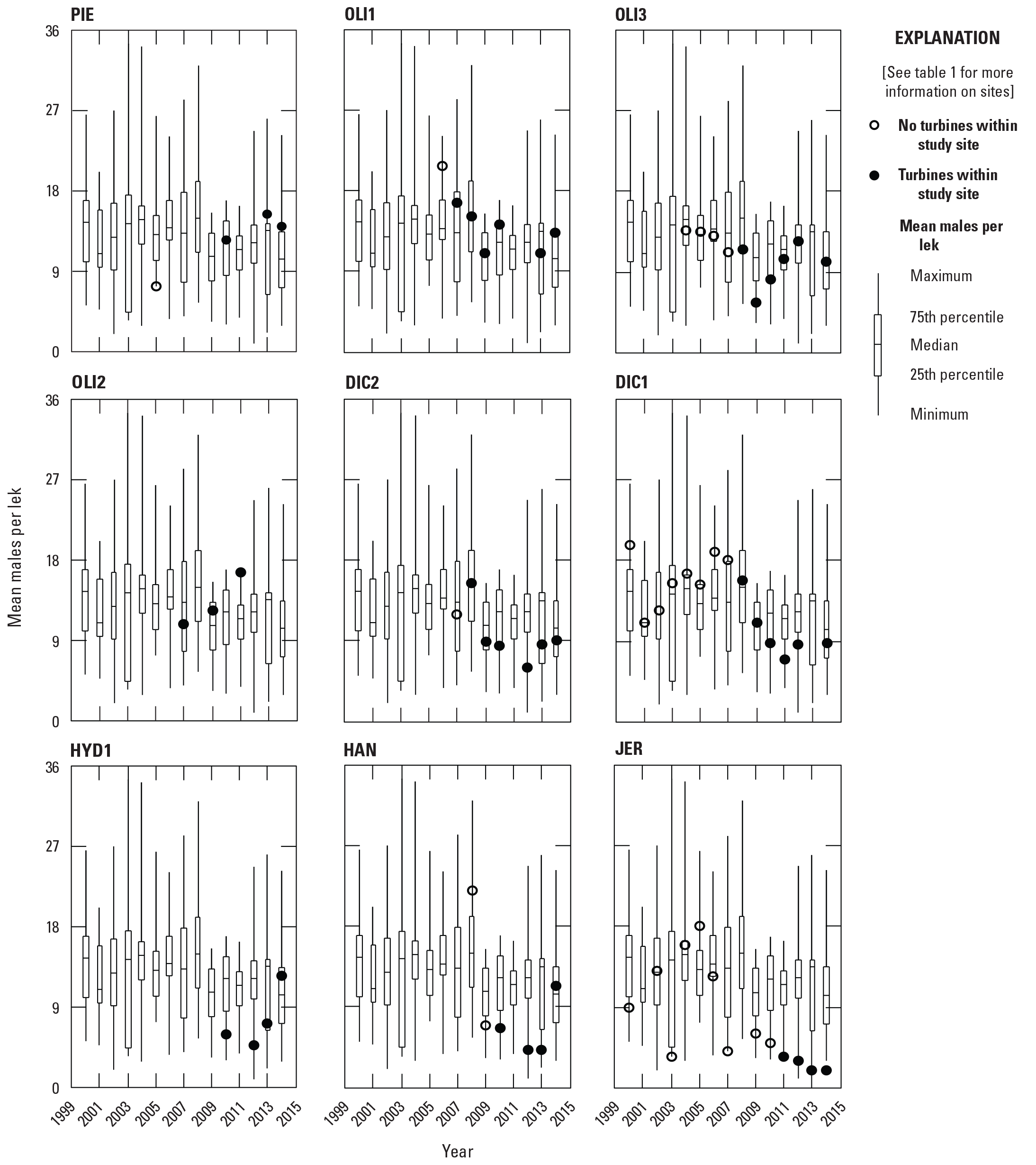
Mean number of sharp-tailed grouse (Tympanuchus phasianellus) males per lek for each of the nine study sites with wind turbines, North Dakota and South Dakota, 2000–14. Boxplots within each panel show summary statistics for nonturbine sites; they are the same in each panel. The circles within each panel indicate the values of mean number of males per lek for the turbine site.
Table 8.
Yearly least squares means (standard error) for lek density and mean number of males for study sites with turbines and without turbines in North Dakota, for sharp-tailed grouse (Tympanuchus phasianellus).[n, number of observations; weighting was done by square root of number years for each study site]
Table 9.
Yearly least squares means (standard error) for lek density and mean number of males for study sites with turbines and without turbines in South Dakota, for sharp-tailed grouse (Tympanuchus phasianellus).[n, number of observations; weighting was done by square root of number years for each study site]
Discussion
We assessed the feasibility of using existing lek survey data gathered by the USGS, NDGF, SDDGFP, USFS, and WEST to answer whether wind facilities affect lek density and mean number of males per lek at the township scale. We determined that data available for the years we assessed had limited utility for our objectives; however, the estimates of lek density and mean number of males per lek can be used for general assessments, such as for planning future surveys or studies. For example, simulations using the summary statistics provided in this report (for example, least squares means and their respective standard errors) could be useful for performing power analyses to aid in designing future studies. To be able to use annual lek surveys to obtain estimates that reflect statewide trends, we offer the following considerations. For a more accurate estimate of lek density and mean number of males per lek at a statewide level, survey routes established using a random process—and not established only in areas known to have grouse leks—will allow for estimates that can be generalized to the entire State. Surveying near roads, as well as distant from roads, may help avoid the issue of roadside sampling bias (Wellicome and others, 2014). The importance of surveying the entire survey area, not just the areas with known leks, should be communicated to observers. Incorporating verification into the annual data reports that an observer surveyed the entire survey area will aid future researchers in being able to calculate the survey area and thus, calculate values for such metrics as lek density. Recording the absence of grouse for all areas surveyed is as important as recording presence or numbers for calculating lek density. Observers should make the best possible effort to identify the sex of birds present. Only the observer in the field can make that determination, or the best determination, under field circumstances. Any assumptions that have to be made later to assign a sex to birds of unknown sex (such as we did in this report) can affect the accuracy of the estimates. Runia and others (2021) provide an example of a survey methodology that addresses some of the aforementioned points and further allows one to estimate relative abundance of males per lek with confidence limits, as well as ways to improve estimates. A balanced design would require a more even distribution of study sites with turbines and without turbines, spread out equally across the study area. Given the above considerations, the estimates and results reported herein should be considered approximate, as the accuracy of the observed data are unknown. To conduct analyses, we assumed the grouse survey data were unbiased and collected consistently, resulting in reasonable estimates of lek densities and mean number of males per lek.
Given that one of the aims of this study was to assess the effects of wind facilities on sharp-tailed grouse lek density and mean number of males per lek, the inclusion of geographic, land cover, and climate explanatory variables was designed to account for these variables to increase precision in assessing the potential effects of wind turbines. The purpose for the inclusion of the aforementioned group of variables was not to complete a habitat assessment but rather to adjust for the variables in an analysis of covariance framework. Therefore, the range of values of the explanatory variables was to some degree controlled by the study design and location of study sites. For example, the study sites in South Dakota are clustered in the mid-eastern portion of the State (fig. 1), resulting in a small range for the values of Easting and Northing (table 3). This limited range of values for some of the explanatory variables could partially account for the lack of associations detected, as could the lack of inclusion of other explanatory variables that might drive lek density and mean number of males, such as the density of predators or hunting pressure. The largest difference between lek response variables occurred between States; that is, lek density and mean number of males increased as one moved from South Dakota into North Dakota, and as one moved from east to west. These trends likely reflect grassland cover, as the eastern portions of these States have higher cropland coverage than the western portions (Niemuth and others, 2005). These trends also could reflect differences in how and where the States operate grouse surveys. In terms of the south-to-north gradient, Sauer and others (2013) indicate that the mean relative abundance of sharp-tailed grouse increases from South Dakota to North Dakota.
The model selection results were based on a candidate set of models that consisted of all one- and two-variable models (excluding those with highly correlated variables). In any candidate set of models, there will always be a model that is deemed “best” (that is, has the lowest AICC value) relative to the rest of the models in the candidate set; however, this is an indication that a particular model is better relative to other models, rather than an indication of how well the model fits the data. Therefore, model fit needs to be assessed. For analyses presented in this report, plots of observed versus predicted values indicated that the best model in each case was a poor predictive model. Plots of the variables that were most important in models and the response variables (figs. 4–9) also showed a lack of association between the explanatory variables and the response variables. Therefore, within this study area and at the scale at which these variables were measured, little to no association was determined between explanatory variables and the response variables.
In this study, an area the size of a township was selected as the experimental unit. This level was deemed reasonable because it was similar to the areal coverage of the NDGF and SDDGFP surveys. If lek density is the metric of interest, then a large area in which multiple leks can be detected, such as a township, is required to compute lek density. For other research questions or metrics of interest, a differently sized experimental unit (for example, a Public Land Survey System section or a lek) may be more appropriate. For example, if assessing habitat use at the lek level, then the lek would be the experimental unit, and habitat variables would be measured at the lek level.
The goal of this study was to assess effects of wind turbine facilities; however, after examining the distribution of the turbine and nonturbine sites (fig. 1), it was clear that such an assessment was not reliable for the following reasons. There were only nine study sites that had turbines, and the year in which turbines were installed varied among these study sites. Although some study sites had data prior to turbine construction, others did not. The total number of years that were surveyed before and after turbines were constructed also varied. The turbine study sites were clustered into five locations (fig. 1), and there were not always good study sites nearby without turbines (to serve as controls) for which surveys had been conducted the same years as the turbine study sites. With a proper design, it would be possible to overcome most of these issues. For example, if data are collected from turbine sites before and after turbine construction and are collected from nearby control sites during the same years, then a Before-After-Control-Impact design can be used to assess the effects of the wind facility. If there are multiple turbine sites and turbines are constructed in different years across the different sites, then a Before-After-Control-Impact design with a staggered entry might be a possibility. Therefore, even though the goal of this study was to assess turbine effects, we concluded this was not feasible with existing data.
Summary
To assess the feasibility of using independently derived, long-term datasets gathered in North Dakota and South Dakota to determine whether wind facilities affected lek metrics, the U.S. Geological Survey obtained six datasets and identified 37 study sites, 9 of which contained wind turbines at varying densities. An association between explanatory variables that described geographic, landscape, and climatic attributes and two primary response metrics that described lekking activity within study sites—lek density (leks per square kilometer) and mean number of males per lek—was examined. The explanatory variables included number of turbines, geographic location, elevation, land-cover attributes available from satellite-derived land-cover data, soil moisture, precipitation, and temperature. Owing to low sample sizes of constructed wind facilities available at the time of analysis, advanced statistical techniques were not able to be used, and the estimates for lek density and mean number of males per lek should be considered approximations. Strong associations were not found between the explanatory variables and response variables. The strongest association was that lek density and mean number of males per lek increased from South Dakota to North Dakota. Owing to the highly unbalanced distribution of turbine and nonturbine study sites across the study area, the analysis with wind turbines was inconclusive.
Acknowledgments
We thank Adam Ryba, U.S. Fish and Wildlife Service, for providing the impetus to initiate this study on wind-energy effects on prairie grouse. We thank Clayton Derby, Ruben Mares, Aaron Robinson, and Travis Runia for providing data. Funding was provided by Acciona Energy, NextEra Energy, the U.S. Fish and Wildlife Service, and the U.S. Geological Survey. We are indebted to field personnel who surveyed leks. Land and wind-facility access was permitted by Acciona Energy, NextEra Energy, site managers, and landowners. Betty Euliss, Eric Smith, Garrett MacDonald, and U.S. Fish and Wildlife Service personnel provided technical and logistical support. We thank Jesse Kolar and Neal Niemuth, U.S. Geological Survey, for insightful comments on earlier versions of this report.
References Cited
Allison, T.D., Diffendorfer, J.E., Baerwald, E.F., Beston, J.A., Drake, D., Hale, A.M., Hein, C.D., Huso, M.M., Loss, S.R., Lovich, J.E., Strickland, M.D., Williams, K.A., and Winder, V.L., 2019, Impacts to wildlife of wind energy siting and operation in the United States: Issues in Ecology, Report No. 21, accessed December 2021 at https://www.esa.org/wp-content/uploads/2019/09/Issues-in-Ecology_Fall-2019.pdf.
Bakker, K.K., 2005, South Dakota all bird conservation plan: Pierre, South Dakota, Wildlife Division Report 2005–09, 131 p., accessed April 2023 at https://gfp.sd.gov/UserDocs/nav/bird-plan.pdf.
Connelly, J.W., Gratson, M.W., and Reese, K.P., 2020, Sharp-tailed Grouse (Tympanuchus phasianellus) (ver. 1.0), in Poole, A.F., and Gill, F.B., eds., The birds of the world: Ithaca, N.Y., Cornell Lab of Ornithology, accessed April 2023 at https://doi.org/10.2173/bow.shtgro.01.
Daly, C., Halbleib, M., Smith, J.I., Gibson, W.P., Doggett, M.K., Taylor, G.H., Curtis, J., and Pasteris, P.P., 2008, Physiographically sensitive mapping of climatological temperature and precipitation across the conterminous United States: International Journal of Climatology, v. 28, no. 15, p. 2031–2064. [Also available at https://doi.org/10.1002/joc.1688.]
Díaz, S., Settele, J., Brondízio, E., Ngo, H., Guèze, M., Agard, J., Arneth, A., Balvanera, P., Brauman, K., Butchart, S., Chan, K., Garibaldi, L., Ichii, K., Liu, J., Subrmanian, S., Midgley, G., Miloslavich, P., Molnár, Z., Obura, D., Pfaff, A., Polasky, S., Purvis, A., Razzaque, J., Reyers, B., Chowdhury, R., Shin, Y., Visseren-Hamakers, I., Wilis, K., and Zayas, C., 2019, Summary for policymakers of the global assessment report on biodiversity and ecosystem services of the Intergovernmental Science-Policy Platform on Biodiversity and Ecosystem Services: Bonn, Germany, IPBES Secretariat, accessed April 2023 at https://uwe-repository.worktribe.com/output/1493508/summary-for-policymakers-of-the-global-assessment-report-onbiodiversity-and-ecosystem-services-of- the-intergovernmental-science-policy-platformon-biodiversity-and-ecosystem-services.
Fink, D., Auer, T., Johnston, A., Strimas-Mackey, M., Robinson, O., Ligocki, S., Hochachka,W., Jaromczyk, L., Wood, C., Davies, I., Iliff, M., and Seitz, L., 2021, eBird status and trends, data version—2020: Ithaca, N.Y., Cornell Lab of Ornithology, accessed December 2021 at https://doi.org/10.2173/ebirdst.2020.
Flanders-Wanner, B.L., White, G.C., and McDaniel, L.L., 2004, Weather and prairie grouse—Dealing with effects beyond our control: Wildlife Society Bulletin, v. 32, no. 1, p. 22–34. [Also available at https://doi.org/10.2193/0091-7648(2004)32[22:WAPGDW]2.0.CO;2.]
Gregory, A.J., McNew, L.B., Prebyl, T.J., Sandercock, B.K., and Wisely, S.M., 2011, Hierarchical modeling of lek habitats of Greater Prairie-Chickens, chap. 2 of Sandercock, B.K., Martin, K., and Segelbacher, G., eds., Ecology, conservation, and management of grouse: Berkeley, Calif., University of California Press, Studies in Avian Biology, v. 39, p. 21–32. [Also available at https://doi.org/10.1525/9780520950573-004.]
Hamilton, S., and Manzer, D., 2011, Estimating lek occurrence and density for sharp-tailed grouse, chap. 3 of Sandercock, B.K., Martin, K., and Segelbacher, G., eds., Ecology, conservation, and management of grouse: Berkeley, Calif., University of California Press, Studies in Avian Biology, v. 39, p. 33–49.
Harrison, J.O., Brown, M.B., Powell, L.A., Schacht, W.H., and Smith, J.A., 2017, Nest site selection and nest survival of Greater Prairie-Chickens near a wind energy facility: The Condor, v. 119, no. 4, p. 659–672. [Also available at https://doi.org/10.1650/CONDOR-17-51.1.]
Hiller, T.L., McFadden, J.E., Powell, L.A., and Schacht, W.H., 2019, Seasonal and interspecific landscape use of sympatric Greater Prairie‐Chickens and Plains Sharp‐tailed Grouse: Wildlife Society Bulletin, v. 43, no. 2, p. 244–255. [Also available at https://doi.org/10.1002/wsb.966.]
Hovick, T.J., Dahlgren, D.K., Papes, M., Elmore, R.D., and Pitman, J.C., 2015, Predicting Greater Prairie-Chicken lek site suitability to inform conservation actions: PLoS One, v. 10, no. 8, e0137021. [Also available at https://doi.org/10.1371/journal.pone.0137021.]
Intergovernmental Panel on Climate Change, 2022, Summary for policymakers, in Pörtner, H.-O., Roberts, D.C., Tignor, M., Poloczanska, E.S., Mintenbeck, K., Alegría, A., Craig, M., Langsdorf, S., Löschke, S., Möller, V., Okem, A., and Rama, B., eds., Climate change 2022—Impacts, adaptation and vulnerability: Cambridge University Press: Cambridge, United Kingdom and New York, N.Y., Contribution of Working Group II to the Sixth Assessment Report of the Intergovernmental Panel on Climate Change, p. 3–33. [Also available at https://doi.org/10.1017/9781009325844.001https://www.ipcc.ch/report/ar6/wg2/downloads/report/IPCC_AR6_WGII_SummaryForPolicymakers.pdf.]
Jamison, B.E., Igl, L.D., Shaffer, J.A., Johnson, D.H., Goldade, C.M., and Euliss, B.R., 2020, The effects of management practices on grassland birds—Lesser Prairie-Chicken (Tympanuchus pallidicinctus), chap. D of Johnson, D.H., Igl, L.D., Shaffer, J.A., and DeLong, J.P., eds., The effects of management practices on grassland birds: U.S. Geological Survey Professional Paper 1842, 36 p., accessed April 2023 at https://doi.org/10.3133/pp1842D.
Lark, T.J., Salmon, J.M., and Gibbs, H.K., 2015, Cropland expansion outpaces agricultural and biofuel policies in the United States: Environmental Research Letters, v. 10, no. 4, 12 p. [Also available at https://doi.org/10.1088/1748-9326/10/4/044003.]
Lark, T.J., Spawn, S.A., Bougie, M., and Gibbs, H.K., 2020, Cropland expansion in the United States produces marginal yields at high costs to wildlife: Nature Communications, v. 11, no. 4295, 11 p. [Also available at https://doi.org/10.1038/s41467-020-18045-z.]
Lloyd, J.D., Aldridge, C.L., Allison, T.D., LeBeau, C.W., McNew, L.B., and Winder, V.L., 2022, Prairie grouse and wind energy–The state of the science and implications for risk assessment: Wildlife Society Bulletin, v. 46, no. 3, 15 p. [Also available at https://doi.org/10.1002/wsb.1305.]
Niemuth, N.D., and Boyce, M.S., 2004, Influence of landscape composition on sharp-tailed grouse lek location and attendance in Wisconsin pine barrens: Ecoscience, v. 11, no. 2, p. 209–217. [Also available at https://doi.org/10.1080/11956860.2004.11682826.]
Niemuth, N.D., Estey, M.E., and Loesch, C.R., 2005, Developing spatially explicit habitat models for grassland bird conservation planning in the Prairie Pothole Region of North Dakota, in Ralph, C.J., and Rich, T.D., eds., Bird conservation implementation and integration in the Americas—Proceedings of the third International Partners in Flight Conference: Albany, Calif., U.S. Dept. of Agriculture, Forest Service, General Technical Report PSW-GTR-191, p. 469–477.
Niemuth, N.D., Walker, J.A., Gleason, J.S., Loesch, C.R., Reynolds, R.E., Stephens, S.E., and Erickson, M.A., 2013, Influence of wind turbines on presence of Willet, Marbled Godwit, Wilson’s Phalarope and Black Tern on wetlands in the Prairie Pothole Region of North Dakota and South Dakota: Waterbirds, v. 36, no. 3, p. 263–276. [Also available at https://doi.org/10.1675/063.036.0304.]
National Oceanic and Atmospheric Administration, 2023, Palmer Drought Severity Index: National Centers for Environmental Information, National Oceanic and Atmospheric Administration database, accessed October 2023 at https://www.ncei.noaa.gov/access/monitoring/historical-palmers/.
Oregon State University, 2014, PRISM Climate Group: Corvallis, Oregon, Oregon State University, accessed December 2020 at https://prism.oregonstate.edu.
Palmer, W.C., 1965, Meteorological drought: Washington, D.C., U.S. Weather Bureau, National Oceanic and Atmospheric Administration, Library and Information Services Division, Research Paper No. 45, 58 p., accessed July 2014 at https://www.droughtmanagement.info/literature/USWB_Meteorological_Drought_1965.pdf.
Proett, M., Roberts, S.B., Horne, J.S., Koons, D.N., and Messmer, T.A., 2019, Columbian Sharp-tailed Grouse nesting ecology—Wind energy and habitat: The Journal of Wildlife Management, v. 83, no. 5, p. 1214–1225. [Also available at https://doi.org/10.1002/jwmg.21673.]
Renfrew, R.B., and Ribic, C.A., 2002, Influence of topography on density of grassland passerines in pastures: American Midland Naturalist, v. 147, no. 2, p. 315–325. [Also available at https://doi.org/10.1674/0003-0031(2002)147[0315:IOTODO]2.0.CO;2.
Rowland, M.M., 2019, The effects of management practices on grassland birds—Greater Sage-Grouse (Centrocercus urophasianus), chap. B of Johnson, D.H., Igl, L.D., Shaffer, J.A., and DeLong, J.P., eds., The effects of management practices on grassland birds: U.S. Geological Survey Professional Paper 1842, 50 p., accessed April 2023 at https://doi.org/10.3133/pp1842B.
Runia, T.J., Solem, A.J., Niemuth, N.D., and Barnes, K.W., 2021, Spatially explicit habitat models for prairie grouse—Implications for improved population monitoring and targeted conservation: Wildlife Society Bulletin, v. 45, no. 1, p. 36–54. [Also available at https://doi.org/10.1002/wsb.1164.]
Sauer, J.R., Link, W.A., Fallon, J.E., Pardieck, K.L., and Ziolkowski, D.J., Jr., 2013, The North American Breeding Bird Survey 1966–2011—Summary analysis and species accounts: North American Fauna, v. 79, p. 1–32. [Also available at https://doi.org/10.3996/nafa.79.0001.]
Schenbeck, G.L., and Moravek, G.E., 1988, Administrative discussions on monitoring Sharp-tailed Grouse courtship display grounds, as a means to determine yearly populations of a forest management plan indicator species: Chadron, Nebr., U.S. Forest Service, Nebraska National Forest, Fort Pierre National Grassland, 2 p.
Schindler, A.R., Haukos, D.A., Hagen, C.A., and Ross, B.E., 2020, A multispecies approach to manage effects of land cover and weather on upland game birds: Ecology and Evolution, v. 10, no. 24, p. 14330–14345. [Also available at https://doi.org/10.1002/ece3.7034.]
Shaffer, J.A., and Buhl, D.A., 2016, Effects of wind-energy facilities on breeding grassland bird distributions: Conservation Biology, v. 30, no. 1, p. 59–71. [Also available at https://doi.org/10.1111/cobi.12569.]
Stevens, B.S., Conway, C.J., Knetter, J.M., Roberts, S.B., and Donnelly, P., 2023, Multi‐scale effects of land cover, weather, and fire on Columbian sharp‐tailed grouse: The Journal of Wildlife Management, v. 87, no. 2, e22349. [Also available at https://doi.org/10.1002/jwmg.22349.]
Stonehouse, K.F., Shipley, L.A., Lowe, J., Atamian, M.T., Swanson, M.E., and Schroeder, M.A., 2015, Habitat selection and use by sympatric, translocated Greater Sage-Grouse and Columbian Sharp-tailed Grouse: The Journal of Wildlife Management, v. 79, no. 8, p. 1308–1326. [Also available at https://doi.org/10.1002/jwmg.990.]. https://doi.org/10.1002/jwmg.990.
Svedarsky, W.D., Toepfer, J.E., Westemeier, R.L., Robel, R.J., Igl, L.D., and Shaffer, J.A., 2022, The effects of management practices on grassland birds—Greater Prairie-Chicken (Tympanuchus cupido pinnatus), chap. C of Johnson, D.H., Igl, L.D., Shaffer, J.A., and DeLong, J.P., eds., The effects of management practices on grassland birds: U.S. Geological Survey Professional Paper 1842, 53 p., accessed April 2023 at https://doi.org/10.3133/pp1842C.
U.S. Department of Agriculture, 2011, Cropland data layer: Washington, D.C., National Agriculture Statistics Service, accessed July 2014 at https://www.nass.usda.gov/Research_and_Science/Cropland/SARS1a.php.
U.S. Department of Energy, 2022, Land-based wind market report—2022 edition: Washington, D.C., Office of Energy Efficiency & Renewable Energy, Report DOE/GO-102022-5763, accessed April 2023 at https://doi.org/10.2172/1893263.
U.S. Energy Information Administration, 2023, Issues in focus—Inflation Reduction Act cases in the AEO2023: Washington, D.C., U.S. Energy Information Administration, Annual Energy Outlook 2023, accessed April 2023 at https://www.eia.gov/outlooks/aeo/IIF_IRA/.
U.S. Fish and Wildlife Service, 2012, U.S. Fish and Wildlife Service land-based wind energy guidelines: Washington, D.C., U.S. Fish and Wildlife Service, accessed April 2023 at https://www.fws.gov/media/land-based-wind-energy-guidelines.
U.S. Geological Survey, 2005, 30-meter resolution National Elevation Dataset: Sioux Falls, S. Dak., U.S. Geological Survey Earth Resources Observation and Science (EROS) Center, accessed April 2023 at https://doi.org/10.5066/F7DF6PQS.
Wellicome, T.I., Kardynal, K.J., Franken, R.J., and Gillies, C.S., 2014, Off-road sampling reveals a different grassland bird community than roadside sampling—Implications for survey design and estimates to guide conservation: Avian Conservation & Ecology, v. 9, no. 1, p. 4. [Also available at https://doi.org/10.5751/ACE-00624-090104.]
Williams, C.K., Ives, A.R., Applegate, R.D., and Ripa, J., 2004, The collapse of cycles in the dynamics of North American grouse populations: Ecology Letters, v. 7, no. 12, p. 1135–1142. [Also available at https://doi.org/10.1111/j.1461-0248.2004.00673.x.]
Wilsey, C., Taylor, L., Bateman, B., Jensen, C., Michel, N., Panjabi, A., and Langham, G., 2019, Climate policy action needed to reduce vulnerability of conservation-reliant grassland birds in North America: Conservation Science and Practice, v. 1, no. 4, p. e21. [Also available at https://doi.org/10.1111/csp2.21.]
Wimberly, M.C., Janssen, L.L., Hennessy, D.A., Luri, M., Chowdhury, N.M., and Feng, H., 2017, Cropland expansion and grassland loss in the eastern Dakotas—New insights from a farm-level survey: Land Use Policy, v. 63, p. 160–173. [Also available at https://doi.org/10.1016/j.landusepol.2017.01.026.]
Winder, V.L., McNew, L.B., Gregory, A.J., Hunt, L.M., Wisely, S.M., and Sandercock, B.K., 2014, Space use by female Greater Prairie-Chickens in response to wind energy development: Ecosphere, v. 5, no. 1, p. 1–17. [Also available at https://doi.org/10.1890/ES13-00206.1.]
Wright, C.K., and Wimberly, M.C., 2013, Recent land use change in the Western Corn Belt threatens grasslands and wetlands: Proceedings of the National Academy of Sciences of the United States of America, v. 110, no. 10, p. 4134–4139. [Also available at https://doi.org/10.1073/pnas.1215404110.]
Appendix 1. Correlation Tables of Explanatory Variables
Table 1.1.
Correlation matrix (Pearson correlation coefficients) of explanatory variables used to develop models for sharp-tailed grouse (Tympanuchus phasianellus) lek density and average number of males per lek in North Dakota and South Dakota, 2000–14. Values are combined for North Dakota and South Dakota. Variable definitions are provided in table 2.[—Left]Table 1.2.
Correlation matrix (Pearson correlation coefficients) of explanatory variables used to develop models for sharp-tailed grouse (Tympanuchus phasianellus) lek density and average number of males per lek in North Dakota, 2000–14. Variable definitions are provided in table 2.[—Left]Table 1.3.
Correlation matrix (Pearson correlation coefficients) of explanatory variables used to develop models for sharp-tailed grouse (Tympanuchus phasianellus) lek density and average number of males per lek in South Dakota, 2000–14. Variable definitions are provided in table 2.[—Left]Conversion Factors
International System of Units to U.S. customary units
Datums
Vertical coordinate information is referenced to the North American Datum of 1983 (NAD 83).
Horizontal coordinate information is referenced to the North American Datum of 1983 (NAD 83).
Elevation, as used in this report, refers to distance above the vertical datum.
Abbreviations
<
less than
AICC
Akaike’s Information Criterion for small samples
ΔAICC
difference of AICC for model minus AICC from model with the lowest AICC value
GPS
Global Positioning System
NASS
National Agricultural Statistical Service
NDGF
North Dakota Game and Fish Department
PDSI
Palmer Drought Severity Index
PRISM
Parameter-elevation Regressions on Independent Slopes Model
SDDGFP
South Dakota Department of Game, Fish and Parks
USFS
U.S. Forest Service
USGS
U.S. Geological Survey
For more information about this publication, contact:
Director, USGS Northern Prairie Wildlife Research Center
8711 37th Street Southeast
Jamestown, ND 58401
701–253–5500
For additional information, visit: https://www.usgs.gov/centers/npwrc
Publishing support provided by the
Rolla Publishing Service Center
Disclaimers
Any use of trade, firm, or product names is for descriptive purposes only and does not imply endorsement by the U.S. Government.
Although this information product, for the most part, is in the public domain, it also may contain copyrighted materials as noted in the text. Permission to reproduce copyrighted items must be secured from the copyright owner.
Suggested Citation
Shaffer, J.A., Buhl, D.A., and Newton, W.E., 2023, Assessing the use of long-term lek survey data to evaluate the effect of landscape characteristics and wind facilities on sharp-tailed grouse lek dynamics in North Dakota and South Dakota: U.S. Geological Survey Open-File Report 2023–1091, 33 p., https://doi.org/10.3133/ofr20231091.
ISSN: 2331-1258 (online)
Study Area
| Publication type | Report |
|---|---|
| Publication Subtype | USGS Numbered Series |
| Title | Assessing the use of long-term lek survey data to evaluate the effect of landscape characteristics and wind facilities on sharp-tailed grouse lek dynamics in North Dakota and South Dakota |
| Series title | Open-File Report |
| Series number | 2023-1091 |
| DOI | 10.3133/ofr20231091 |
| Publication Date | December 12, 2023 |
| Year Published | 2023 |
| Language | English |
| Publisher | U.S. Geological Survey |
| Publisher location | Reston, VA |
| Contributing office(s) | Northern Prairie Wildlife Research Center |
| Description | Report: v, 33 p.; Data Release |
| Country | United States |
| State | North Dakota, South Dakota |
| Online Only (Y/N) | Y |
| Additional Online Files (Y/N) | N |