

Database and Time Series of Nearshore Waves Along the Alaskan Coast from the United States-Canada Border to the Bering Sea
Links
- Document: Report (6 MB pdf) , HTML , XML
- Data Release: USGS Data Release - Nearshore wave time-series along the coast of Alaska computed with a numerical wave model
- NGMDB Index Page: National Geologic Map Database Index Page (html)
- Download citation as: RIS | Dublin Core
Abstract
Alaska’s Arctic coast has some of the highest coastal erosion rates in the world, primarily driven by permafrost thaw and increasing wave energy. In the Arctic, a warming climate is driving sea ice cover to decrease in space and time. A lack of long-term observational wave data along Alaska’s coast challenges the ability of engineers, scientists, and planners to study and address threats and effects from wave-driven erosion and flooding. To overcome the lack of available observational wave data in the nearshore in this study by the U.S. Geological Survey (USGS), waves were downscaled with the Simulating WAves Nearshore numerical wave model (SWAN) for the hindcast period of 1979 to 2019 from the United States-Canada border to the Bering Sea utilizing nine model domains. For each domain, the model was forced at the open boundary with 2,500 representative “sea states,” which are likely combinations of significant wave heights, mean wave periods, mean wave directions, and wind speeds and directions. The sea states were obtained from the European Centre for Medium-Range Weather Forecasts “ERA5” dataset for reanalysis of winds and waves using a multivariant maximum-dissimilarity algorithm. The SWAN runs created a downscaled wave database at each grid point, which was used to reconstruct the 40-year time series in the nearshore along the 5- and 10-meter (m) isobaths at locations approximately 400 m apart and corresponding to transects spaced approximately 50 m alongshore, as developed for USGS shoreline-change assessments. Reconstructed time series were compared to observations to validate the numerical model and the downscaled wave database method and showed overall good agreements.
Introduction
Background and Motivation
The changing climate is increasingly impacting coastlines around the world (for example, Vitousek and others, 2017; Storlazzi and others, 2018; Barnard and others, 2019; Oppenheimer and others, 2019; Reguero and others, 2019). One of the most affected regions is the Arctic, which is warming at a faster rate than any other region (Serreze and others, 2009; Cohen and others; 2014; Acosta Navarro and others, 2016). In the Arctic, the warming climate leads to an increase in the duration of the open-water season (the period during which the ocean is not covered by ice) and a delay in ice formation in the fall and winter (Serreze and others, 2009), which is typically the stormy season. Studies have found that the extended open-water season correlates with an increase in maximum and average wave heights (Erikson and others, 2020a; Nederhoff and others, 2022) at offshore locations, whereas in the nearshore the total wave energy over the year increases primarily due to an increase in the extent of the open-water season (Erikson and others, 2020a; Gibbs and others, 2021; Nederhoff and others, 2022).
Increases in wave energy will likely cause an increase in erosion, which in Arctic regions is driven by a combination of wave activity and thermal processes (Erikson and others, 2011; Stopa and others, 2016; Denali Commission, 2019; Gibbs and others, 2019a; Casas‐Prat and Wang, 2020; Erikson and others, 2020a; Gibbs and others, 2021). The American and Canadian coastlines exhibit the highest erosion rates in the Arctic (Lantuit and others, 2012). The United States parts of the Beaufort Sea and Chukchi Sea coastlines have been primarily erosional since the 1940s (Gibbs and Richmond, 2017; Gibbs and others, 2019b). At some locations, coastal erosion rates have more than doubled since the mid-20th century (Frederick and others, 2016; Jones and others, 2020; Gibbs and others, 2021).
To be able to assess past and anticipate future changes to the Alaskan coast, reliable nearshore wave data are needed. However, wave observations are sparse and difficult to obtain due to the harsh environmental conditions and remoteness of the region. Although reanalysis data are now available for the satellite era (1979 to present), the resolution is still too coarse (0.25 degrees for atmospheric and 0.5 degrees for oceanic processes) to capture nearshore processes such as refraction, diffraction, dissipation, and non-linear energy transfer processes, which are important to account for when considering erosion and inundation of coastal areas.
Here, we use a numerical wave model to downscale available reanalysis wave data for the Alaskan region from the United States-Canada border to the Bering Sea (fig. 1). The generated nearshore time series allows for a detailed analysis of changes in the wave climate along the entire coast. We caution, however, that this dataset is based on outdated bathymetry (see the “Bathymetry” section) and should be updated when modern bathymetric nearshore data are made available. The lack of modern nearshore bathymetric data and its importance in modeling coastal hazards along Alaska’s shorelines is well recognized (Denali Commission, 2019; Hamilton, 2021; Williams and Erikson, 2021). Extensive efforts are underway to update the well-outdated (greater than [>] 50 year) nearshore bathymetric data along the roughly 4,000-kilometer (km) stretch of coast that this study addresses, but the data are not anticipated to be available for another 5 to 10 years (Alaska Mapping Executive Committee, 2020). Simultaneously, coastal hazards are of immediate and increasing concern to vulnerable coastal ecosystems and villages, necessitating an understanding of both past and potential future coastal storms. To that end, the scientific community-at-large is at a temporary impasse of either postponing research or moving forward to advance the quantification of nearshore wave conditions, but with the latter action subject to uncertainties in accuracy. This study by the U.S. Geological Survey (USGS) was structured to address these acute needs but with the recognition that uncertainties in the results exist and that updates should be made when modern coastal bathymetry data are obtained.
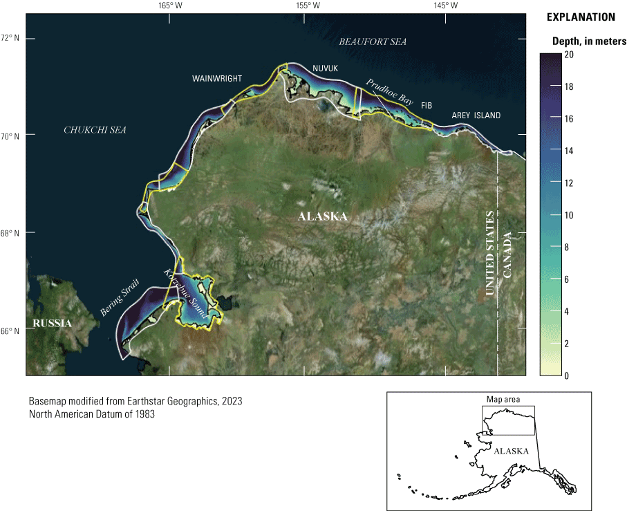
Map of the study area from the United States-Canada border to the Bering Strait, Alaska. Simulations were carried out in stationary mode for 2,500 sea states over eight two-dimensional (2D) curvilinear and one 2D rectangular domains for a total of nine domains. The offshore extent was roughly defined by the 20-meter isobath. Domain lengths varied, depending on local shoreline curvature. The model domains are shown with alternating white and yellow polygons. Observations for model and method validation are available at Wainwright, Foggy Island Bay (FIB), and Arey Island (see section “Nearshore Model-Observation Comparisons,” fig. 6, and table 1 for detailed observation locations).
Data and Methods
Nearshore wave conditions were simulated for the years 1979 to 2019 along the model boundaries from the United States-Canada border to the Bering Strait (fig. 1) by forcing the numerical wave model SWAN (Simulating WAves Nearshore, Booij and others, 1999) with representative wind and sea states (Camus and others, 2011; Reguero and others, 2013), hereafter termed “sea states.” These were derived from 40 years of reanalyzed wind and wave conditions from the European Centre for Medium-Range Weather Forecasts (ECMWF) ERA5 dataset. The results were then used to develop a downscaled wave database (DWDB) from which nearshore time series in 5- and 10-meter (m) water depths were generated by first matching sea states at the boundary with wave and atmospheric conditions at each time-point of a given time series, and then picking the corresponding DWDB values in the nearshore. These steps are also outlined in figure 2, and a validation of the model and the DWDB method is in the “Nearshore Model-Observation Comparisons” section of this report. The use of representative wind and sea states, instead of forcing the wave model with the full time series length (“brute-force method”), allows the model to be run with a lower computational expense.
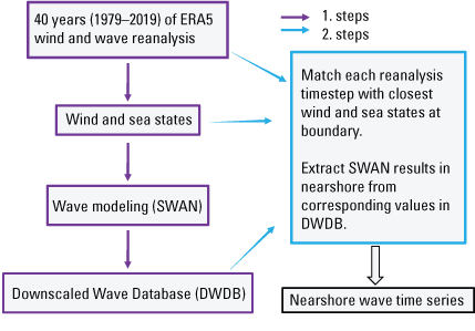
Flow chart outlining the steps involved in constructing the nearshore time series. First, sea states, identified from 40 years of wind and wave reanalysis, were modeled with the numerical wave model SWAN to create a downscaled wave database (DWDB). Second, each time step of the 40-year time series was matched with the closest sea state at the boundary, and values were then extracted from the DWDB in the nearshore.
Meteorological and Oceanic Reanalysis Forcing Data
ERA5 (Hersbach and others, 2020) is a detailed reanalysis of the global atmosphere, land surface, and ocean waves from 1950 onwards produced by the ECMWF. This dataset provides, among other variables, estimates of atmospheric parameters such as air temperature, pressure, and wind on a 0.25-degree grid and sea ice concentrations and information on waves over the global oceans at a 0.5-degree resolution. The reanalysis combines model data with observations from across the world into a globally complete and consistent dataset. ERA5 has been shown to perform well in capturing observed weather and climate variability in Alaska and the Arctic (Graham and others, 2019). Here, offshore significant wave height (Hs), mean period (Tm), and direction (Dm) are used as input to the SWAN model. Wind conditions (u10, v10) from this reanalysis dataset are additionally applied across all model domains. ERA5 does not provide wave conditions if the sea ice cover is greater than 30 percent, therefore the reconstructed time series assumes no waves inshore if there are no waves in ERA5. Additionally, the 0.25-degree sea ice resolution does not resolve landfast ice, which could potentially cause an overestimate of the wave climate (Hošeková and others, 2021).
Nearshore Wave Model
Model hindcasts were run with the third generation, physics-based, phase-averaging wind-wave model SWAN (version 3.07.00.63652). SWAN is based on the wave action balance and includes physical processes such as wind-wave generation, shoaling, breaking, and nonlinear wave-wave interactions (see Booij and others, 1999, for details). Simulations were carried out in a stationary mode for 2,500 sea states (see “Boundary Conditions and Downscaled Wave Database” section of this report) over eight two-dimensional (2D) curvilinear and one 2D rectilinear domains for a total of nine domains (fig. 1). The rectilinear domain was chosen for the Kotzebue Sound area to ensure numerical stability. The offshore extent for the model domains was roughly defined by the 20-m isobath, and the domain length and width varied, depending on the offshore extent of each grid and local shoreline curvature. Selection of the approximately 20-m isobath as the offshore extent was based on (1) the need to reduce computation cost by optimizing the spatial extent in the cross-shore direction while accounting for the shallow and wide continental shelf that abuts the north and west Alaska coastline, and (2) comparisons between ERA5 reanalysis waves and five temporary buoy deployments along the Beaufort Sea part of the Alaska Coast which showed an acceptable accuracy (average root mean square error [RMSE] and bias =0.35 m and 0.16 m respectively; Kasper and others, 2023) in 22- to 30-m water depth, supporting the use of these data as open boundary conditions for the nearshore model. Nearshore grid size resolution was on average less than or equal to [≤] 200×200 m. In the offshore regions, cross-shore grid resolution varied between about 300–1,000 m and 200–300 m in the alongshore direction. Since grid resolution was coarse offshore, due to the large simulation domain, SWAN’s “obstacle” option was used to ensure that barrier islands were properly resolved in areas with larger cell sizes. Obstacles, implemented either as option “dam” or “sheet” with a polyline, can be located between grid cells and interrupt the wave propagation (Deltares, 2020). In this study, dams were used to represent barrier islands, with transmission coefficients depending on (1) the wave conditions at the obstacle and (2) obstacle configuration. Empirical coefficients and that describe obstacle shape, were kept at default values of 2.6 and 0.15, respectively. Wave reflection off the obstacle was set to zero, and the dam height was set to 2 m, on the basis of 2010–2011 light detection and ranging (lidar) elevation measurements along Alaska’s north coast (Gibbs and Richmond, 2017; Hamilton and others, 2021).
SWAN was run with the white capping formulation of van der Westhuysen and others (2007) using 72 directional bins (5-degree resolution) and 46 frequency bands from 0.03 to 2.5 hertz (Hz). The friction formulation of Collins (1972) with a coefficient of 0.02 was used after calibration by Nederhoff and others (2022) for the Alaskan coast. Wave conditions at the boundaries and wind forcing, applied homogenously over each domain, were determined by the ERA5 sea states (see the “Boundary Conditions and Downscaled Wave Database” section in this report). The presence of sea ice was not accounted for in these SWAN model runs. Whereas landfast sea ice conditions are not explicitly accounted for in these runs, the database could be expanded to include nearshore sea ice by running the same conditions with different levels of sea ice cover.
Bathymetry
The bathymetry for the domains was primarily based on products provided by the International Bathymetric Chart of the Arctic Ocean (IBCAO; Jakobsson and others, 2020), which have a resolution of 200×200 m. IBCAO is based on all available bathymetric datasets north of 64° N. latitude. In the nearshore region, these are mostly National Oceanic and Atmospheric Administration (NOAA), National Ocean Service (NOS) hydrographic surveys, which were conducted between the 1940s and 1970s. It is assumed that the vertical IBCAO datum is the chart datum of the NOS samples (Mean Lower Low Water, MLLW), which were converted to mean sea level (MSL) by using datum information from NOAA’s Prudhoe Bay AK station (https://tidesandcurrents.noaa.gov/datums.html?id=9497645). Changes to the bathymetry were made in the vicinity of Cross Island, where a NOS dataset (H07760 from 1950) appeared to have been horizontally misplaced and which was manually rectified. Sea level rise was considered as an increase in water levels of 2 millimeters per year (mm/yr) in the region (Sultan and others, 2011) between the year of the surveys and today (roughly 0.15 m), which was added to the bathymetry. The land boundary is based on data extracted from USGS topographic maps from the 1950s to 1990s at scales between 1:63,360 and 1:250,000.
Inconsistencies between the land boundary and IBCAO products were adjusted by removing bathymetric points along the boundary in a roughly 200- to 400-m-wide section, setting the immediate coastline to zero and using a smoothing process (internal diffusion, see Deltares, 2021) to interpolate between the coastline and nearest bathymetric depths. Some uncertainty in bathymetry and land boundaries exists. In particular, many of the NOS hydrographic surveys in the nearshore region were conducted between the 1940s and 1970s and likely differ in places from current and recent past bathymetry over the simulation time period from 1979 to 2019. Erosion of the coastline and barrier island migration have led to substantial change in the nearshore bathymetry since data were last collected (for example, Bristol and others, 2021; Gibbs and others, 2021; Hamilton and others, 2021). Erosion is especially severe along the United States part of the Beaufort Sea coast, where, for example, shoreline erosion rates measured in the region around Drew Point are as high as 17.2 m/yr in the years between 2007 and 2016 (Jones and others, 2018). In addition, nearshore surveys in the southern Chukchi region are generally sparse (https://www.ncei.noaa.gov/maps/bathymetry/). Overall, uncertainties related to bathymetry and shoreline position are substantial and cannot be specified owing to a lack of knowledge and local differences in erosion and accretion rate. Therefore, the data have been manually inspected and improved where needed and accepted as is for the remainder of this study.
Boundary Conditions and Downscaled Wave Database
Carrying out model computations over the period 1979–2019 along roughly 4,000 km of coastline would be computationally intensive and require considerable time to complete; in other words, it would be very computationally expensive. To improve this, the model was forced with a reduced set of likely combinations of wind and wave parameters, hereafter termed “sea states,” which are used as boundary conditions to the SWAN model domains. These parameters were derived from ERA5 reanalysis time series during the open season (when sea ice cover is less than 30 percent) covering the period 1979 to 2019. For each grid, appropriate ERA5 output locations were chosen along the length of the grid (which ranged from approximately [~] 150 to 280 km in the alongshore direction), and all ERA5 time series were extracted. The number of ERA5 locations varied with grid length and coastline alignment. Those time series were combined for each grid, and representative sea states were established with a multivariant maximum-dissimilarity algorithm (MDA), which determined representative combinations of significant wave height (Hs), mean wave period (Tm), mean wave direction (Dm), wind speed (Wspd), and wind directions (Wdir), resulting in 2,500 different combinations. The MDA method allows for a full representation of the marine climate because the determined sea states are uniformly distributed across all the data (fig. 3), including extreme events (Camus and others, 2011).
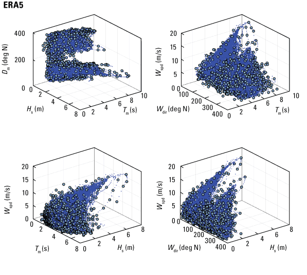
Graphs showing an example of selected sea states across a full distribution of wave and wind conditions at the boundary of a single model domain in the Beaufort Sea, Alaska. The blue dots show the three-dimensional (3D) combinations of wave height (Hs), mean wave period (Tm), mean wave direction (Dm), wind speed (Wspd), and wind direction (Wdir) over the 40-year period from 1979 to 2019. Identified representative sea states, used as boundary conditions to the SWAN model (Booij and others, 1999), are shown with the larger circles. The ERA5 dataset (Hersbach and others, 2020) is a detailed reanalysis of the global atmosphere, land surface, and ocean waves from 1950 onwards produced by the European Centre for Medium-Range Weather Forecasts (ECMWF).
SWAN was forced with all 2,500 wind and sea states to create a DWDB at each grid point. The wind was assumed to be homogenous for each sea state over the model domain. To construct nearshore hindcast time series, the 40-year record of ERA5 hindcasts along the boundary was first matched with sea states. For each timestep, the closest combination, as described below, of significant wave height, mean wave period, mean wave direction, wind speeds, and wind directions to ERA5 was found. The algorithm started with a combination of small differences (Hs less than or equal to [≤] 0.05 m, Tm≤0.5 second [s], Dm≤5 degrees, wind speed <2 meters per second [m/s] and wind direction <5 degrees), and if no sea state could be found, a scheme was deployed that allowed for a gradual widening of the bins up to a difference in Hs of 1 m, in Tm of 2 s, in Dm of 20 degrees, in wind speed of 3 m/s, and in wind direction of 20 degrees. Values for which the difference in Hs is greater than 0.15 m are flagged to inform the user of this difference. Flags are set for differences of 0.20 m, 0.25 m, 0.50 m, 0.75 m, and 1 m. While the MDA method allows for the inclusion of extreme events, values for some timesteps could not be found (less than 0.6 percent of the open season values and mostly coming from about 100 degrees), owing to the limit of 2,500 wind and sea states that were chosen to save computational time. Most missing values were caused by an underrepresentation of the wave direction or wind speed (particularly by wind speeds smaller than 4 m/s) in the sea states. Out of the 52 ERA5 locations that were used for the reconstruction, six locations are missing one to three of the highest 10 wave heights. For all values that could not be found, as well as for times when no ERA5 wave data were available (during the ice-covered season) values were set to −9999. Time steps for which the differences between ERA5 wind or wave directions and the found sea state was equal or larger than 15 degrees were flagged (Flag D) in the time series files (available from Engelstad and others, 2024). Wind and wave directions can considerably affect the wave evolution, especially when varying in the alongshore direction between onshore and offshore, so the user is advised to use caution under these circumstances. Although not all conditions are a perfect match at the boundary (fig. 4) owing to the constraints of using a limited set of sea states instead of running the model brute force, extremes for all parameters are captured well and the difference between the original ERA5 time series and the reconstructed values at the boundary are minimal.
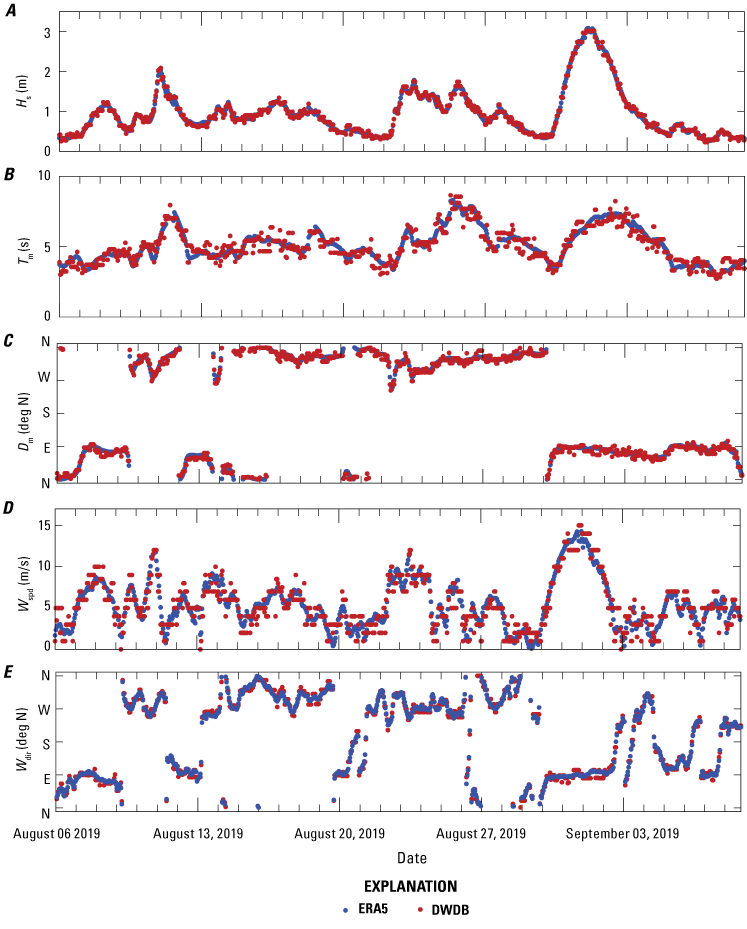
Graphs showing an example of a reconstructed time series at the domain boundary for nearshore waves along the Arctic coast of Alaska. The marine climate at the model boundary is described by A, significant wave height (Hs), B, mean wave period (Tm), C, mean wave direction (Dm), D, wind speed (Wspd), and E, wind direction (Wdir). Blue dots show the ERA5 time series and red dots show the reconstructed time series from the downscaled wave database (DWDB).
For each of the sea states found at the boundary, the corresponding values were extracted from the DWDB at nearshore locations. Those nearshore locations were determined from shore-normal transects derived by the USGS for shoreline change studies (Gibbs and Richmond, 2017) using the Digital Shoreline Analysis System (DSAS) extension for ArcGIS (Thieler and others, 2017). These transects cover the open-ocean and barrier coast as well as the lagoon coast. Approximately every 8th transect of the roughly 50-m alongshore spaced transects was chosen for an alongshore resolution of roughly 400 m. Data were extracted from the DWDB along the 5-m and 10-m isobath closest to each selected transect (fig. 5). For the reconstruction of the time series, the time series of the closest ERA5 locations to each nearshore location was used. Since ERA5 locations are roughly 55 km apart, wave and wind time series between ERA5 locations can differ substantially. This, in turn, can cause inconsistencies between nearshore time series for adjacent output locations that utilize time series from two different ERA5 locations (see fig. 5). To make this apparent to users, adjacent nearshore locations using different ERA5 locations are marked by a flag, Flag S, in the time series files. In addition, Flag S is also used when adjacent nearshore locations were located in separate numerical domains, which can cause inconsistencies even with a wide grid overlap (dual transect locations were removed roughly midpoint of the grid overlap).
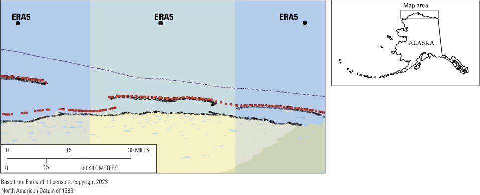
Diagram showing the matching of transects, output locations, and ERA5 locations for the reconstruction of nearshore wave time series for the Arctic coast of Alaska. For roughly every 8th transect of the 50-meter (m) Digital Shoreline Analysis System (DSAS) transects (black lines), the closest output locations on the 5-m isobath (red dots) were found. Next, the wave and wind time series of the closest ERA5 location to each output location was used to reconstruct the time series. The affiliation of output locations with ERA5 locations is exemplified by the different shading. The 20-m isobath is shown as a blue line.
Although the method of reconstructing the time series was described above for the 40-year hindcast, data can be extracted from the DWDB in a short amount of time at every location on the grid for any period within the DWDB time frame.
Nearshore Model Observation Comparisons
The SWAN model and DWDB method were validated with observations. In situ wave and wind measurements, or observations, are available for nearshore locations in the vicinity of Foggy Island Bay for the years 2019 and 2020 (Kasper and others, 2023; fig. 6, table 1), for a nearshore location near Wainwright for the year 2009 (data from Erikson and others, 2022), and near Arey Island for the year 2011 (Erikson and others, 2020b). Additionally, a historical dataset containing wave height and directional observations from the 1985 “Endicott study” is available (Envirosphere, 1991). Additionally, the DWDB method was compared to the “brute-force method.”
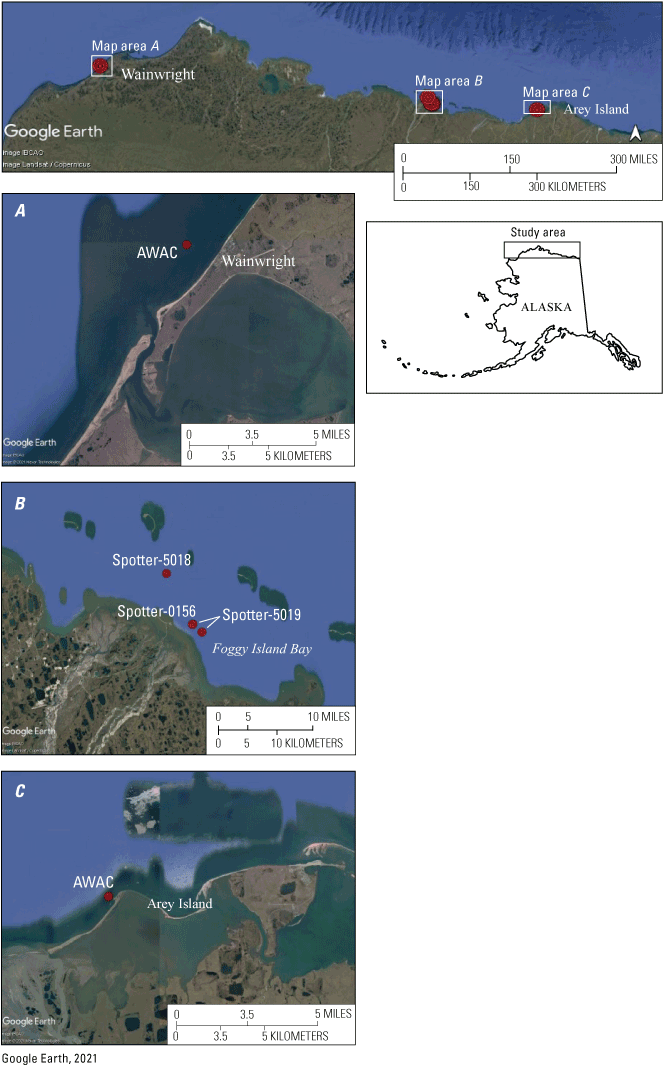
Images showing nearshore wave observation locations along the Arctic coastline of Alaska on the Beaufort Sea. The upper panel shows an overview of the wave observation locations (red circles). The lower panels are close-ups showing the instrumentations at these locations (for more information see table 1). AWAC, Nortek acoustic wave and current profiler; Spotter, Sofar wave buoys.
Table 1.
Overview of wave observations used for model-data comparison along the Arctic coastline of Alaska on the Beaufort Sea.[Figure 6 shows the nearshore wave observation locations. Note that in 2020 the SPOT 0519 buoy was displaced during the measurement campaign, probably by an ice float. “F” in F18, F22, F24, and F27 stands for “fyke,” which was the name used in the Endicott study, available from Envirosphere (1991). Spotter, Sofar wave buoys; AWAC, Nortek 1-MHz acoustic wave and current profiler; FIB, Foggy Island Bay; N, north; W, west; Hz, hertz; m, meter; min, minute; ~, approximate; UAF, University of Alaska, Fairbanks; USGS, U.S. Geological Survey].
The combined implementation of the model and DWDB was assessed by calculating several statistical test scores. The mean-absolute error (MAE) between model results and observations was calculated as
where Further, the root-mean-square error (RMSE) was estimated as whereas the scatter index (SCI), is a relative measure of the RMSE compared to the variability in the observations. The model bias was calculated as the mean difference between model and observations.Foggy Island Bay
Observations in the summers of 2019 and 2020 (table 1) in the vicinity of Foggy Island Bay were collected by the University of Alaska Fairbanks, with Sofar Spotter devices (Raghukumar and others, 2019). These buoys measure 3D surface displacements at 2.5 Hz. Bulk wave statistics, such as significant wave heights, mean and peak wave periods, and mean and peak wave directions, are computed from the surface elevation variance density spectrum every 30 minutes in the frequency range from 0.0293 to 0.6543 Hz. Note that in 2020 the Foggy Island Bay Spotter buoy (SPOT 0519) was displaced during the measurement campaign, probably by an ice float (fig. 6, table 1). Wave measurements at Wainwright were obtained by the USGS with a Nortek 1-MHz acoustic wave and current profiler (AWAC), sampling during 8.53-minute bursts at a rate of 2 Hz, (fig. 6, table 1) from the end of August to the beginning of October 2009. Wave measurements at Arey Island were collected in August of 2011 with a Nortek 1-MHz AWAC, sampling at 1 Hz in 17-minute-long hourly bursts.
The comparison between SWAN results and observations in Foggy Island Bay in 2019 shows good agreement (fig. 7) for Hs, Tm, and Dm, suggesting that the model can reproduce the wave field in the area. Skill scores for wave heights are 0.12 m and 0.09 m for the RMSE and MAE, respectively (table 2), and the SCI is 24 percent. Wave periods have a RMSE of 0.8 seconds (s), a MAE of 0.5 s, and a SCI of 23 percent. Further, SWAN runs with the DWDB method have similar reproductive skill as the more elaborate and time-consuming brute-force method (fig. 7). Skill score differences for Hs between the two methods are 0.01 m for the RMSE, 0.01 m for MAE and a bias of 0.03 m, and the SCI is the same. For Tm, the difference between the two methods is 0.1 s for the RMSE, 3 percent for the SCI and a −0.1 s bias, and the MAE is the same. The largest discrepancies in Hs between model(s) and observations can be seen between August 31 and September 2, 2019. Although it is possible that SWAN was not able to reproduce the onset of the sudden large wave events, for example, owing to the stationary mode with hourly wind forcing, the strong increase in measured wave heights over short periods of time (for example, from Hs=0.85 m on September 2, 20:30 hour to Hs=2.34 m on September 2, 21:00 hour) suggests that the difference could also have been caused by measurement errors. Also note that the ERA5 wind speed used to force the model was higher by roughly 4 to 5 m/s during this period (fig. 7D). Smaller mismatches between modeled and observed Hs, such as on August 26, September 4, and September 8, are mostly caused by differences between ERA5 winds (which, as mentioned earlier, were forced homogenously over the SWAN domain) and local winds, as supported by a model run using the local wind forcing (not shown).
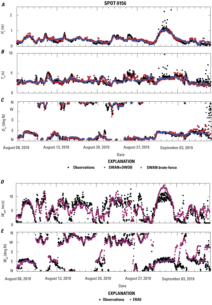
Wave and wind model-to-observation comparisons for SPOT 0156 at Foggy Island Bay, Alaska, in 2019. Simulating WAves Nearshore (SWAN) model output created with the brute-force method are compared to the downscaled wave database (DWDB) method. A, Comparison of wave heights (Hs), B, mean wave periods (Tm), and C, mean wave directions (Dm) for the time series created with the DWDB (red dots), observations (black dots) collected in Foggy Island Bay, and a brute-force model run (blue dots). D, offshore wind speed (Wspd), and E, direction (Wdir) from ERA5 (magenta dots) are compared to local winds measured by the Spotter Sofar wave buoy (black dots).
Table 2.
Model skill statistics for wave heights and wave periods for instruments near Foggy Island Bay (SPOT 0156, SPOT 0518, and SPOT 0519), Wainwright (F1), and Arey Island (BI01), Alaska.[Statistics from downscaled wave database (DWDB) and brute-force (BF) methods are provided for all locations except Wainwright, for which no brute-force run was conducted. DWDB average is the average of the statistics calculated for the DWDB method. Hs, wave height; m, meter; MAE, mean-absolute error; RMSE, root mean square error; s, second; SCI, scatter index; Tm, wave period; —, no data; %, percent].
The wind also seems to affect the comparison of modeled and observed Hs at the SPOT 0518 and SPOT 0519 locations in 2020 (figs. 8, 9). Discrepancies between modeled and observed Hs can be seen for times of disagreements between ERA5 and local winds (see, for example, July 25, July 29–August 1, and August 7 in figs. 8, 9). On the other hand, the largest event with wave heights up to 1 m on August 2, for which ERA5 and local winds were similar, was captured well by the DWDB method, but it was underpredicted by the brute-force model run for SPOT 0518. Although the discrepancy in wind speeds was largest (~5 m/s) around July 27, the wind direction was from the southwest and did not affect wind-wave growth as much because the fetch (the area where the wind blows to generate waves) was limited. In general, modeled and observed Tm agreed well (figs. 8B, 9B), aside from some single higher than modeled periods, as between July 30–31 when Tm for SPOT 0518 was as high as 12 s, whereas modeled Tm was around 2 s. This was not observed for SPOT 0519. Wave directions were mostly aligned with the wind directions, and differences between modeled and observed Dm (figs. 8C, 9C) are apparent when local and ERA5 wind fields differ.
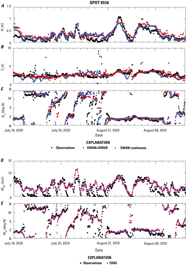
Wave and wind model-to-observation comparisons for SPOT 0518 near Foggy Island Bay, Alaska, in 2020. Simulating WAves Nearshore (SWAN) model output created with the brute-force method is compared with the downscaled wave database (DWDB) method. A, Comparison of wave heights (Hs), B, mean wave periods (Tm), and, C, mean wave directions (Dm) for the time series created with the DWDB (red dots), observations (black dots), and a brute-force model run (blue dots). D, Offshore wind speed (Wspd), and, E, direction (Wdir) from ERA5 (magenta dots) are compared to local winds measured by the Spotter Sofar wave buoy (black dots).
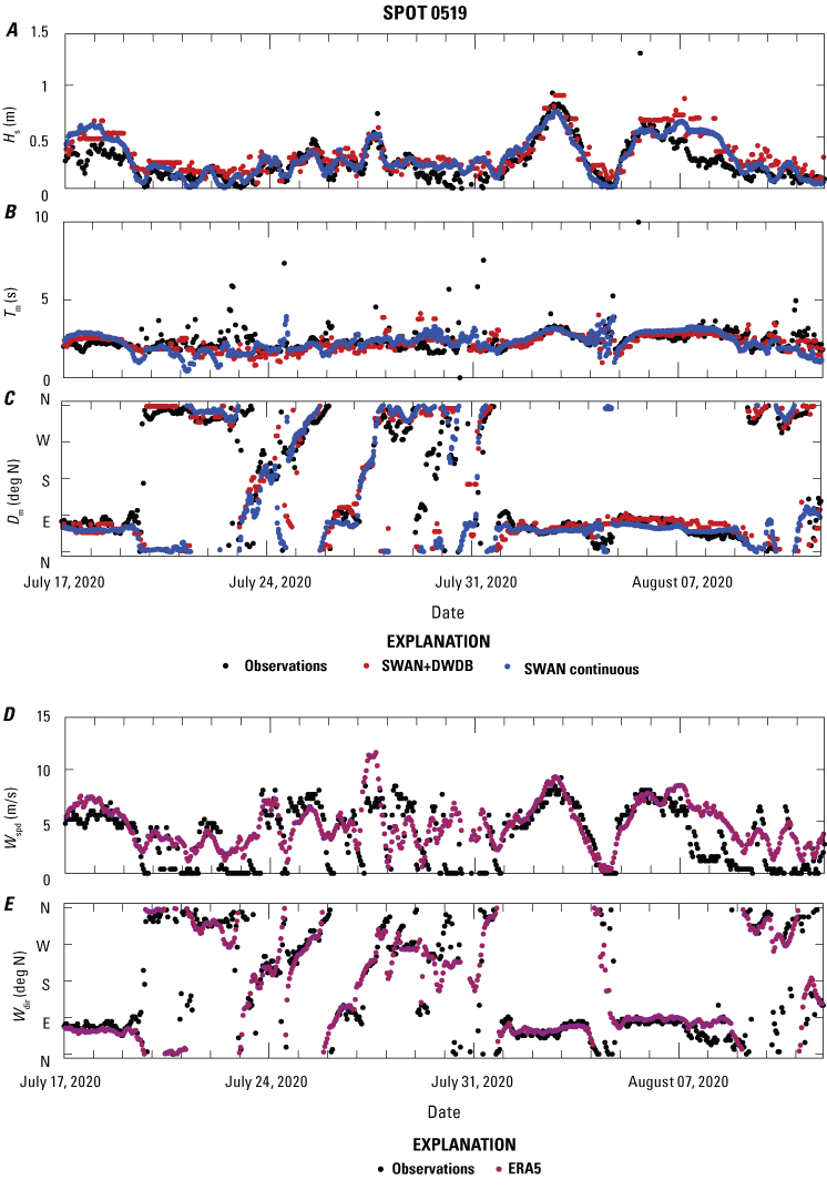
Wave and wind model-to-observation comparisons for SPOT 0519 at Foggy Island Bay, Alaska, in 2020. Simulating WAves Nearshore (SWAN) model output created with the brute-force method is compared with the downscaled wave database (DWDB) method. A, Comparison of wave heights (Hs), B, mean wave periods (Tm), and, C, mean wave directions (Dm) for the time series created with the DWDB (red dots), observations (black dots), and a brute-force model run (blue dots). D, Offshore wind speed (Wspd), and, E, direction (Wdir) from ERA5 (magenta dots) are compared to local winds measured by the Spotter Sofar wave buoy (black dots).
Wainwright
Observations are also available (Erikson and others, 2022) for a location (F1) in the Chukchi Sea fronting the community of Wainwright (table 1, fig. 6). Although for this location, small and medium Hs (~1 m) are generally captured well by the model (fig. 10), larger events in the period from September 2–8, 2009, were underestimated, with the largest difference on September 4 of about 0.9 m. Those differences are likely generated by variations in observed water levels (water levels were kept constant in the SWAN runs) owing to the wind direction (fig. 11), which are not captured by the model because wind speed and directions implemented in the model agree well with local wind observations (National Centers for Environmental Information, n.d.) at Wainwright airport at this time (fig. 11C, D). Generally, wind from the east tends to decrease water levels, whereas winds from the west tend to increase water levels along the North Slope (Reimnitz and Maurer, 1979; Sultan and others, 2011; Erikson and others, 2020a). This is caused by the Coriolis force, which deflects wind- and wave-forced currents to the right of the flow direction. Additionally, strong winds can push water masses downwind, which at the Wainwright location could also potentially increase water levels at times when the wind is from the west and decrease water levels when the wind is from the east. On the other hand, wave heights were overestimated on September 22 by about 0.5 m, which could have been caused by a lower than modeled wind speed and (or) by the lower water level owing to the easterly winds (fig. 11B, C). Water level fluctuations coinciding with a mismatch between model and observations are not noticed for the other locations in the vicinity of Foggy Island Bay, which are sheltered by barrier islands, whereas the Wainwright location is fully exposed to the open ocean but close to shore.
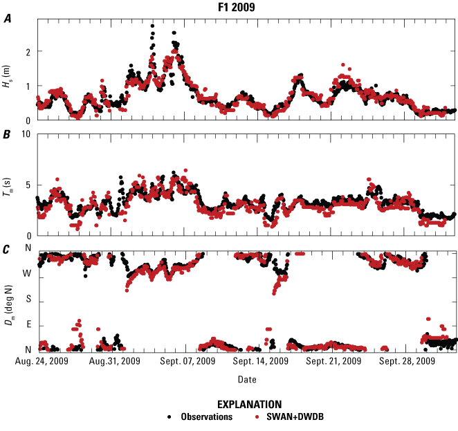
Wave model-to-observation comparisons at F1, near Wainwright, Alaska, in 2009. Simulating WAves Nearshore (SWAN) model output created with the brute-force method is compared to the downscaled wave database (DWDB) method. A, Comparison of wave heights (Hs), B, mean wave periods (Tm), and C, mean wave directions (Dm) for the time series created from the DWDB (red dots) and wave observations collected at Wainwright (black dots).
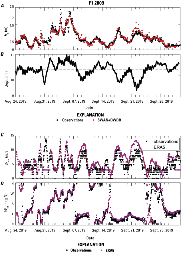
Wave height, water depth, and wind model-to-observation comparisons at Wainwright, Alaska, in 2009. Simulating WAves Nearshore (SWAN) model output created with the brute-force method is compared to the downscaled wave database (DWDB) method. A, Wave heights (Hs) where observed (black dots) and modeled (red dots) values are contrasted to, B, observed variations in water depth (depth), and, C, with offshore wind speed (Wspd) and, D, direction (Wdir) from ERA5 (magenta dots). ERA5 dataset from Hersbach and others (2020). SWAN, Booij and others (1999). Observed winds (black dots) were collected at Wainwright airport and are available from the National Centers for Environmental Information (NCEI) website (n.d.; https://www.ncei.noaa.gov/access/search/data-search/local-climatological-data).
Arey Island
For all previously presented model-data comparisons, the agreement between observations was good or could be explained by differences between ERA5 offshore winds and locally observed winds. In contrast, modeled wave heights offshore of Arey Island at BI01 are consistently biased high by about 0.20 m (fig. 12A) even though DWDB, ERA5, and local winds compare well (fig. 12D, E). The low wave heights (0.50 m) observed during periods of high westerly and easterly sustained winds ≥12 m/s suggest that the measured Hs may be biased low, rather than the model estimating too high. In fact, once a uniform bias correction of 0.19 m is applied, the RMSE reduces from 0.26 to 0.17 m for Hs (table 2). Satellite data indicate that sea ice was more than 300 km offshore, yielding a fetch area larger than 90,000 square kilometers (km2) that is only marginally limiting to wave growth. Simple calculations of wave heights in approximately 5-m water depth using linear wave theory under conditions of 12-m/s winds and an assumed ice-free region indicate that wave heights should be on the order of 1 m, supporting the SWAN model results. Because the SWAN model and the DWDB method provided otherwise good results, this suggests that the difference could be caused by local factors such as changes in bathymetry that are not captured by the model for the particular simulation time.
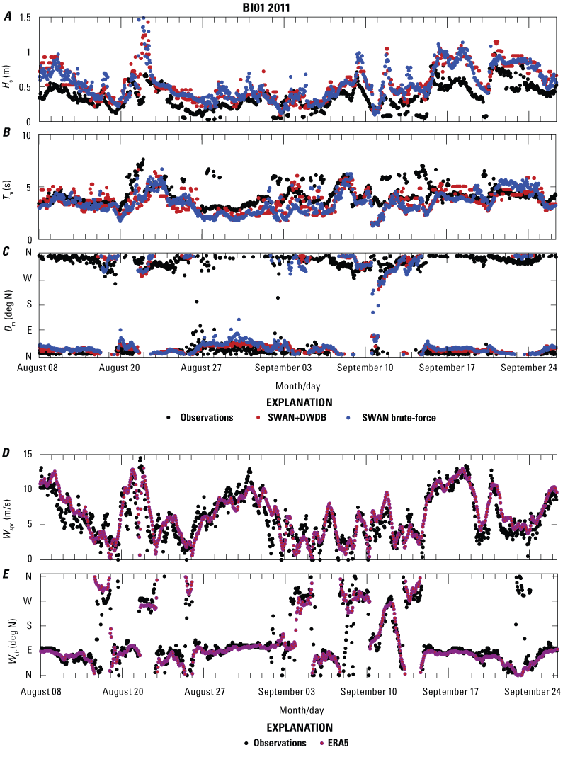
Wave and wind model-to-observation comparisons at BI01, offshore of Arey Island, Alaska, in 2011. Simulating WAves Nearshore (SWAN) model output created with the brute-force method was compared to the downscaled wave database (DWDB) method, whereas local wind observations are compared to ERA5 winds. A, Comparison of wave heights (Hs), B, mean wave periods (Tm), and, C, mean wave directions (Dm) for the time series created with the DWDB (red dots), observations (black dots) collected at Arey Island in 2011, and a model run with brute-force (blue dots). D, Offshore wind speed (Wspd), and, E, direction (Wdir) from ERA5 (magenta dots) are compared to local winds measured (black dots) at Barter Island (National Centers for Environmental Information, n.d.).
The fact that the agreement between observations and model is better for some locations than others is also reflected in the model skills, where the largest spread away from the line of perfect agreement is found for the Arey Island comparison (fig. 13, table 2). Although the model-observation comparison is not perfect, the combined RMSE (table 2) for Hs is relatively small (0.17m) and mostly unbiased (0.09 m). The model-observation comparison shows a larger spread in the data for the combined Tm (SCI of 44 compared to 38 for Hs) for which the bias is small (−0.2 s), although the combined RMSE is 1.7 s. (For statistics regarding the model skill at single locations, see table 2).
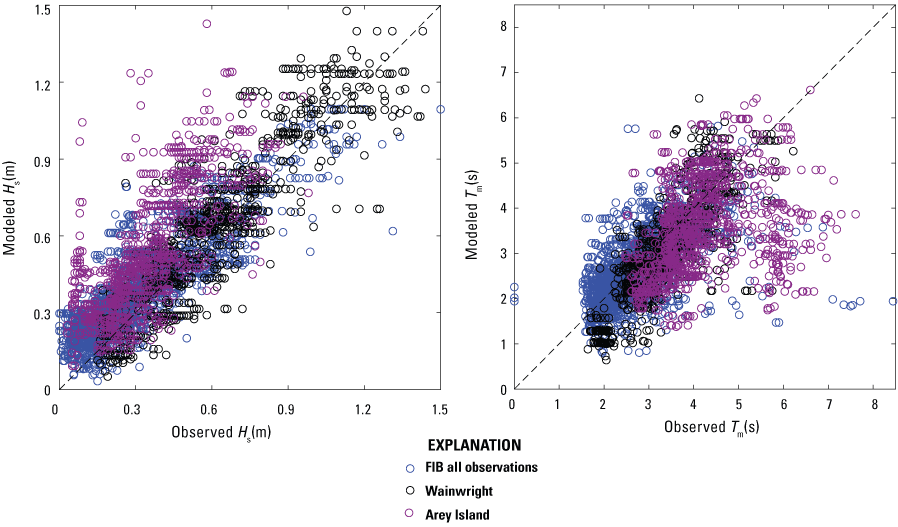
Scatter plots summarizing modeled and measured wave heights and mean wave periods along the Arctic coast of Alaska. A, Modeled and observed wave heights (Hs), and, B, wave mean periods (Tm) grouped by locations. The group “FIB all observations” includes SPOT 0156, SPOT 0518, and SPOT 0519. The dashed black line is the line of perfect agreement. Model skill statistics are in table 2.
Model-Observation Comparison for Historical Wave Observations
The historical observations from 1985 (Envirosphere, 1991) are separated here from the more recent observations introduced above and will not be subjected to a skill performance analysis. The reason is twofold. First, wave height measurements were taken once a day with a wave staff (comparable to a yard stick), whereas the wave direction was determined by measuring the travel direction with a hand-held compass and therefore measurements lack precision. Second, owing to erosional and (or) depositional changes in the area and the construction of Endicott Island in 1987, locations relative to barrier islands and the coastline have changed. However, owing to the sparsity of measurements on the North Slope, these observations are valuable, and we use them to confirm that model results are in the expected value range.
We used 4 out of a total of the 27 measurement locations (fig. 14) for which observed and modeled water depths were similar. Numbers in the location name refer to all historical observation locations and are led by the letter “F,” an abbreviation for the original name “fyke” (meaning a bag net for catching fish). Historical wave heights were measured in 0.1-m increments, whereas wave directions were recorded in 10-degree increments. Wave directions were converted to true north, assuming a magnetic declination of 30 degrees. Although observations are available from July to mid-September, the length of the comparison record is restricted by offshore ERA5 wave conditions, which were only available after September 3 due to offshore ice cover. Each of the daily observed values was compared to the average daily modeled value as well as the minimum and maximum daily values (fig. 15).
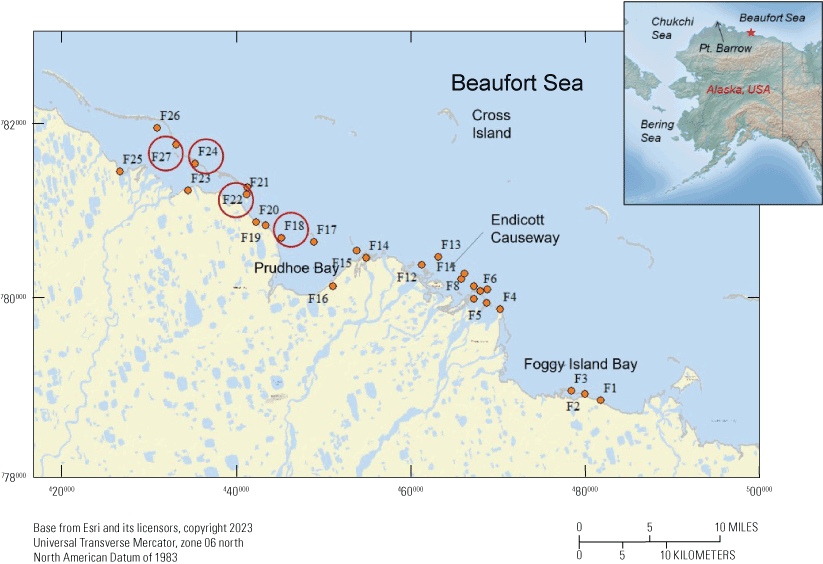
Map showing all locations of data for model comparisons to historical wave-staff wave measurements collected in 1985 (Envirosphere, 1991) from Foggy Island Bay to west of Prudhoe Bay, Alaska. Numbers indicate all historical observation locations and refer to the location names, which consist of a leading “F” (an abbreviation for original name “fyke”). Red circles mark the four locations chosen for the model-data comparison used in this study. Background image from World Street Map by Esri (https://doc.arcgis.com/en/data-appliance/6.4/maps/world-street-map.htm).
Overall, the model-observation comparison shows fair results (fig. 15) considering the measurement methods, uncertainties in bathymetry, and local changes in barrier island locations. While the comparison certainly shows some discrepancies between observations and model (such as for wave heights at F24 and wave directions at F27, see fig. 15), differences are still within an order of magnitude. F18, located furthest away from the barrier islands, shows the best agreement between observations and model. Additionally, the highest observed wave heights (0.6 m), measured at F22, are represented by the model.
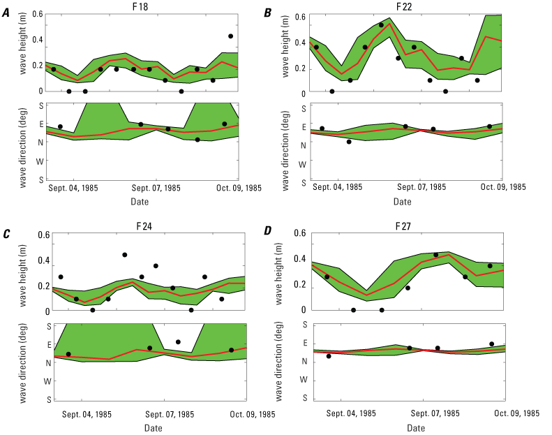
Plots comparing observations of historical wave heights and directions from 1985 to model output at four locations (latitudes and longitudes can be inferred from table 1) west of Foggy Island Bay, Alaska. Observation-location names consist of a leading “F” (an abbreviation for original name “fyke”), followed by a number (see fig. 14 and table 1 for exact locations). Historical wave height and direction observations are crude estimates that were collected once daily with a “wave staff” (comparable to a yard stick) and a hand-held compass. A–D, Observations (black dots) are compared to modeled averages (red line) in daily wave heights and wave directions. The shaded green area shows the extent of modeled minimum and maximum daily values.
Products
Three hourly hindcasted (1979–2019) time series of Hs, Tm, and Dm were generated for 6,399 locations between the United States-Canada border and the Bering Strait. These locations are approximately 400 m apart and correspond to transects used in USGS shoreline change assessments. Data are available from a USGS data release that accompanies this report (Engelstad and others, 2024). These data are presented as netCDF files at the 5- and 10-m isobaths and are packaged for the Beaufort Sea region from the United States-Canada border to Nuvuk (Point Barrow), for the Chukchi Sea region from Nuvuk to Kotzebue Sound, and from Kotzebue Sound to the Bering Strait.
Flags included in the dataset advise caution (where necessary) when using these data. Flag D is used for time steps when the wave and (or) wind directions at the model boundary differ by more than 15 degrees between the ERA5 hindcast data and the value used from the downscaled wave database. Flag S indicates possible inconsistencies between adjacent time series locations, caused by either the use of different offshore ERA5 hindcast locations, or by a switch from one numerical model domain to another (see “Boundary Conditions and Downscaled Wave Database” section). For both flags, 1 indicates this condition is true and 0 indicates that it is not true. Additionally, values for which the difference in Hs is greater than 0.15 m are flagged to inform the user of this difference. Flags are set for differences of 0.20 m, 0.25 m, 0.50 m, 0.75 m, and 1 m.
Summary
Climate change impacts the Arctic Alaskan coastline, which has some of the highest erosion rates in the world. Erosion in the Arctic is primarily driven by permafrost thaw and wave activity. Studies have found that the warming climate is causing the open-water season (the period during which the ocean is not covered by ice) to be longer. This is because warmer temperatures cause more sea ice to melt, leaving greater areas of open water and the sea ice to melt earlier and refreeze later in the year. This means that (1) waves can increase in height because the most severe storms occur in the fall and winter, and (2) the total wave energy increases because winds can transfer energy to the waves for a longer period and across larger ocean water-surface areas. More wave energy will likely cause more coastal erosion. Not many meteorological and wave data are available along the Alaskan Arctic coast that can be used to study past changes and anticipate future changes. Simultaneously, coastal hazards are of immediate and increasing concern to vulnerable coastal ecosystems and villages. To fill the wave data gap, we used a numerical wave model, driven by hindcasted winds and medium- to deep-water waves, to provide time series of wave heights, wave periods, and wave directions within nearshore shallow regions from the United States-Canada border to the Bering Sea for years 1979 to 2019. The model accounts for physical processes that are important in the nearshore, such as the refraction of waves and the dissipation of wave energy. Because the U.S. Arctic coastline from the Canadian border to the Bering Sea is approximately 4,000 kilometers long, simulating 40 years would take a long time. To reduce computation times, we developed a database of nearshore wave conditions from 2,500 combinations of wave heights, mean wave periods, mean wave directions, and winds that represent the offshore wave climate over the past 40 years. These representative “sea states” were established for each of the nine model domains that were utilized to run the nearshore coastal models. The results of those model runs created a downscaled wave database (DWDB), which, in turn, was used to recreate the 40-year time series at locations along the coast that are approximately 400 meters (m) apart and in 5- and 10-m water depths. The resulting hindcasted nearshore time series is derived from downscaling offshore ERA5 reanalysis wave conditions for times when sea ice concentrations were less than 30 percent, and it assumes static still water levels and no landfast sea ice. The uncertainty in wave heights associated with water level variations due to storm surges and astronomic tides are estimated to be ±30 percent along the 5-m isobath (for water level variations of ±3 m in the study region). The lack of landfast sea ice likely overestimates coastal wave exposure during spring and summer break up and fall season refreeze (as such, the user is cautioned on using the full time series for estimating annual absolute cumulative wave energy). Improvements to the results could be derived by expanding the developed database to include varying states of landfast ice and interrogating the database with higher resolution nearshore sea ice conditions; however, high resolution sea ice products that date back to 1979 are, to the knowledge of the authors, not available at this time. The model and methodology were validated by comparing reconstructed time series with available observational wave data (typically during times of little to no landfast ice), which showed overall good agreement.
Acknowledgments
We would like to thank Alexander Nereson (U.S. Geological Survey) for providing the manually rectified National Oceanic and Atmospheric Administration National Ocean Service dataset (H07760) from 1950.
References Cited
Acosta Navarro, J.C., Varma, V., Riipinen, I., Seland, Ø., Kirkevåg, A., Struthers, H., Iversen, T., Hansson, H.-C., and Ekman, A.M.L., 2016, Amplification of Arctic warming by past air pollution reductions in Europe: Nature Geoscience, v. 9, no. 4, p. 277–281, accessed December 21, 2021, at https://doi.org/10.1038/ngeo2673.
Alaska Mapping Executive Committee, 2020, Mapping the coast of Alaska—A 10-year strategy in support of the United States economy, security, and environment: Alaska Coastal Mapping Strategy, accessed December 19, 2021, at https://alaska-coastal-mapping-strategy-dewberry.hub.arcgis.com/.
Barnard, P.L., Erikson, L.H., Foxgrover, A.C., Hart, J.A.F., Limber, P., O’Neill, A.C., van Ormondt, M., Vitousek, S., Wood, N., Hayden, M.K., and Jones, J.M., 2019, Dynamic flood modeling essential to assess the coastal impacts of climate change: Scientific Reports, v. 9, no. 1, article 4309, accessed December 20, 2021, at https://doi.org/10.1038/s41598-019-40742-z.
Bristol, E.M., Connolly, C.T., Lorenson, T.D., Richmond, B.M., Ilgen, A.G., Choens, R.C., Bull, D.L., Kanevskiy, M., Iwahana, G., Jones, B.M., and McClelland, J.W., 2021, Geochemistry of coastal permafrost and erosion-driven organic matter fluxes to the Beaufort Sea near Drew Point, Alaska: Frontiers in Earth Science (Lausanne), v. 8, article 598933, 13 p., https://doi.org/10.3389/feart.2020.598933.
Booij, N., Ris, R.C., and Holthuijsen, L.H., 1999, A third-generation wave model for coastal regions—1. Model description and validation: Journal of Geophysical Research, v. 104, no. C4, p. 7649–7666, accessed November 21, 2021, at https://doi.org/10.1029/98JC02622.
Camus, P., Méndez, F.J., and Medina, R., 2011, A hybrid efficient method to downscale wave climate to coastal areas: Coastal Engineering, v. 58, no. 9, p. 851–862, accessed December 11, 2021, at https://doi.org/10.1016/j.coastaleng.2011.05.007.
Casas‐Prat, M., and Wang, X.L., 2020, Projections of extreme ocean waves in the Arctic and potential implications for coastal inundation and erosion: Journal of Geophysical Research Oceans, v. 125, no. 8, article e2019JC015745, 18 p., accessed February 21, 2021, at https://doi.org/10.1029/2019JC015745.
Cohen, J., Screen, J., Furtado, J., Barlow, M., Whittleston, D., Coumou, D., Francis, J., Dethloff, K., Entekhabi, D., Overland, J., and Jones, J., 2014, Recent Arctic amplification and extreme mid-latitude weather: Nature Geoscience, v. 7, no. 9, p. 627–637, accessed December 21, 2020, at https://doi.org/10.1038/ngeo2234.
Collins, J.I., 1972, Prediction of shallow-water spectra: Journal of Geophysical Research, v. 77, no. 15, p. 2693–2707, accessed November 21, 2020, at https://doi.org/10.1029/JC077i015p02693.
Deltares, 2020, Delft3D, Waves—User Manual: Delft, Netherlands, Deltares, 153 p., accessed May 13, 2020, at https://content.oss.deltares.nl/delft3d/manuals/Delft3D-WAVE_User_Manual.pdf.
Deltares, 2021, QUICKIN, ver. 4.04.01 Delft, Netherlands, Deltares, accessed May, 2021, at https://content.oss.deltares.nl/delft3d/manuals/QUICKIN_User_Manual.pdf.
Denali Commission, 2019, Identification of threats from erosion, flooding, and thawing permafrost in remote Alaska communities: Denali Commission, prepared by University of Alaska Fairbanks Institute of Northern Engineering, U.S. Army Corps of Engineers Alaska District, U.S. Army Corps of Engineers Cold Regions Research and Engineering Laboratory, Report INE19.03, 96 p., accessed at https://www.denali.gov/wp-content/uploads/2019/11/Statewide-Threat-Assessment-Final-Report-November-2019-1-2.pdf.
Engelstad, A.C., Erikson, L.H., Reguero, B.G., Gibbs, A.E., and Nederhoff, K., 2024, Nearshore wave time series along the coast of Alaska computed with a numerical wave model: U.S. Geological Survey data release, https://doi.org/10.5066/P931CSO9.
Erikson, L.H., Storlazzi, C.D., Collins, B.D., Hatcher, G.A., Reiss, T.E., and Engelstad, A.C., 2022, Hydrographic and sediment field data collected in the vicinity of Wainwright, Alaska, in 2009: U.S. Geological Survey data release, https://doi.org/10.5066/P94V9W0S.
Erikson, L.H., Storlazzi, C.D., and Jensen, R.E., 2011, Wave climate and trends along the Eastern Chukchi Arctic Alaska coast, in Wallendorf, L.A., Jones, C., Ewing, L., and Battalio, R., eds., Solutions to Coastal Disasters 2011, Anchorage, Alaska, June 25–29, 2011, Proceedings: American Society of Civil Engineers (ASCE), p. 273–285, accessed December 09, 2020, at https://doi.org/10.1061/41185(417)25.
Erikson, L.H., Gibbs, A.E., Richmond, B.M., Storlazzi, C.D., Jones, B.M., and Ohman, K.A., 2020a, Changing storm conditions in response to projected 21st century climate change and the potential impact on an Arctic barrier island-lagoon system—A pilot study for Arey Island and Lagoon, eastern Arctic Alaska: U.S. Geological Survey Open-File Report 2020–1142, 68 p., accessed December 21, 2021, at https://doi.org/10.3133/ofr20201142.
Erikson, L.H., Gibbs, A.E., Richmond, B.M., Jones, B.M., Storlazzi, C.D., and Ohman, K.A., 2020b, Modeled 21st century storm surge, waves, and coastal flood hazards, and supporting oceanographic and geological field data (2010 and 2011) for Arey and Barter Islands, Alaska and vicinity: U.S. Geological Survey data release, https://doi.org/10.5066/P9LGYO2Q.
Frederick, J.M., Thomas, M.A., Bull, D.L., Jones, C.A., and Roberts, J.D., 2016, The Arctic coastal erosion problem: U.S. Department of Energy, National Nuclear Security Administration, prepared by Sandia National Laboratories, Albuquerque, N. Mex., report no. SAND2016-9762, 122 p., accessed December 01, 2021, at https://doi.org/10.2172/1431492.
Gibbs, A.E., and Richmond, B.M., 2017, National assessment of shoreline change—Summary statistics for updated vector shorelines and associated shoreline change data for the north coast of Alaska, U.S.-Canadian border to Icy Cape: U.S. Geological Survey Open-File Report 2017–1107, 21 p., accessed December 13, 2021, at https://doi.org/10.3133/ofr20171107.
Gibbs, A.E., Nolan, M., Richmond, B.M., Snyder, A.G., and Erikson, L.H., 2019a, Assessing patterns of annual change to permafrost bluffs along the North Slope coast of Alaska using high-resolution imagery and elevation models: Geomorphology, v. 336, p. 152–164, accessed January 21, 2021, at https://doi.org/10.1016/j.geomorph.2019.03.029.
Gibbs, A.E., Snyder, A.G., and Richmond, B.M., 2019b, National assessment of shoreline change—Historical shoreline change along the north coast of Alaska, Icy Cape to Cape Prince of Wales: U.S. Geological Survey Open-File Report 2019–1146, 52 p., accessed January 21, 2021, at https://doi.org/10.3133/ofr20191146.
Gibbs, A.E., Erikson, L.H., Jones, B.M., Richmond, B.M., and Engelstad, A.C., 2021, Seven decades of coastal change at Barter Island, Alaska—Exploring the importance of waves and temperature on erosion of coastal permafrost bluffs: Remote Sensing, v. 13, no. 21, article 4420, 25 p., https://doi.org/10.3390/rs13214420.
Graham, R.M., Hudson, S.R., and Maturilli, M., 2019, Improved performance of ERA5 in Arctic gateway relative to four global atmospheric reanalyses: Geophysical Research Letters, v. 46, no. 11, p. 6138–6147, accessed January 05, 2021, at https://doi.org/10.1029/2019GL082781.
Hamilton, A.I., Gibbs, A.E., Erikson, L.H., and Engelstad, A.C., 2021, Assessment of barrier island morphological change in northern Alaska: U.S. Geological Survey Open-File Report 2021–1074, 28 p., accessed January 21, 2022, at https://doi.org/10.3133/ofr20211074.
Hersbach, H., Bell, B., Berrisford, P., Hirahara, S., Horányi, A., Muñoz-Sabater, J., Nicolas, J., Peubey, C., Radu, R., Schepers, D., Simmons, A., Soci, C., Abdalla, S., Abellan, X., Balsamo, G., Bechtold, P., Biavati, G., Bidlot, J., Bonavita, M., Chiara, G., Dahlgren, P., Dee, D., Diamantakis, M., Dragani, R., Flemming, J., Forbes, R., Fuentes, M., Geer, A., Haimberger, L., Healy, S., Hogan, R.J., Hólm, E., Janisková, M., Keeley, S., Laloyaux, P., Lopez, P., Lupu, C., Radnoti, G., Rosnay, P., Rozum, I., Vamborg, F., Villaume, S., and Thépaut, J.-N., 2020, The ERA5 global reanalysis: Quarterly Journal of the Royal Meteorological Society, v. 146, no. 730, p. 1999–2049, accessed January 23, 2021, at https://doi.org/10.1002/qj.3803.
Hošeková, L., Eidam, E., Panteleev, G., Rainville, L., Rogers, W. E., and Thomson, J., 2021, Landfast ice and coastal wave exposure in northern Alaska: Geophysical Research Letters, v. 48, no. 22, article e2021GL095103, accessed October 11, 2023, at https://doi.org/10.1029/2021GL095103.
Jakobsson, M., Mayer, L.A., Bringensparr, C., Castro, C.F., Mohammad, R., Johnson, P., Ketter, T., Accettella, D., Amblas, D., An, L., Arndt, J.E., Canals, M., Casamor, J.L., Chauché, N., Coakley, B., Danielson, S., Demarte, M., Dickson, M.-L., Dorschel, B., Dowdeswell, J.A., Dreutter, S., Fremand, A.C., Gallant, D., Hall, J.K., Hehemann, L., Hodnesdal, H., Hong, J., Ivaldi, R., Kane, E., Klaucke, I., Krawczyk, D.W., Kristoffersen, Y., Kuipers, B.R., Millan, R., Masetti, G., Morlighem, M., Noormets, R., Prescott, M.M., Rebesco, M., Rignot, E., Semiletov, I., Tate, A.J., Travaglini, P., Velicogna, I., Weatherall, P., Weinrebe, W., Willis, J.K., Wood, M., Zarayskaya, Y., Zhang, T., Zimmermann, M., and Zinglersen, K.B., 2020, The international bathymetric chart of the Arctic Ocean (vers. 4.0): Scientific Data, v. 7, article 176, 14 p., accessed January 13, 2021, at https://doi.org/10.1038/s41597-020-0520-9.
Jones, B.M., Farquharson, L.M., Baughman, C., Buzard, R.M., Arp, C.D., Grosse, G., Bull, D.L., Günther, F., Nitze, I., Urban, F., Kasper, J.L., Frederick, J.M., Thomas, M.A., Jones, C., Mota, A., Dallimore, S., Tweedie, C.E., Maio, C.V., Mann, D.H., Richmond, B.M., Gibbs, A.E., Xiao, M., Sachs, T., Iwahana, G., Kanevskiy, M.Z., and Romanovsky, V.E., 2018, A decade of remotely sensed observations highlight complex processes linked to coastal permafrost bluff erosion in the Arctic: Environmental Research Letters, v. 13, no. 11, article 115001, 14 p., accessed January 22, 2021, at https://doi.org/10.1088/1748-9326/aae471.
Jones, B.M., Irrgang, A.M., Farquharson, L.M., Lantuit, H., Whalen, D., Ogorodov, S., Grigoriev, M., Tweedie, C., Gibbs, A.E., Strzelecki, M.C., Baranskaya, A., Belova, N., Sinitsyn, A., Kroon, A., Maslakov, A., Vieira, G., Grosse, G., Overduin, P., Nitze, I., Maio, C., Overbeck, J., Bendixen, M., Zagórski, P., and Romanovsky, V.E., 2020, Arctic report card 2020—Coastal permafrost erosion: National Oceanic and Atmospheric Administration, Office of Oceanic and Atmospheric Research, Arctic Report Card, 10 p., accessed January 19, 2021, at https://doi.org/10.25923/e47w-dw52.
Kasper, J., Erikson, L.H., Ravens, T., Bieniek, P., Engelstad, A., Nederhoff, K., Duvoy, P., Fisher, S., Brown, E.P., Yaman, M., Reguero, B., 2023, Central Beaufort Sea wave and hydrodynamic modeling study—Report 1—Field measurements and model development: Anchorage, Alaska, U.S. Department of the Interior, Bureau of Ocean Energy Management, 100 p., report no. OCS Study BOEM 2022-078, contract no. M17AC00020, and IAA no. M17PG00046.
Lantuit, H., Overduin, P.P., Couture, N., Wetterich, W., Aré, F., Atkinson, D., Brown, J., Cherkashov, G., Drozdov, D., Forbes, D.L., Graves-Gaylord, A., Grigoriev, M., Hubberten, H.W., Jordan, J., Jorgenson, T., Ødegård, R.S., Ogorodov, S., Pollard, W.H., Rachold, V., Sedenko, S., Solomon, S., Steenhuisen, F., Streletskaya, I., and Vasiliev, A., 2012, The Arctic coastal dynamics database—A new classification scheme and statistics on Arctic permafrost coastlines: Estuaries and Coasts, v. 35, no. 2, p. 383–400, accessed January 21, 2021, at https://doi.org/10.1007/s12237-010-9362-6.
National Centers for Environmental Information, n.d., U.S. local climatological data (LCD): National Centers for Environmental Information database, accessed January 21, 2021, at https://www.ncei.noaa.gov/access/search/data-search/local-climatological-data.
Nederhoff, K., Erikson, L., Engelstad, A., Bieniek, P., and Kasper, J., 2022, The effect of changing sea ice on wave climate trends along Alaska’s central Beaufort Sea coast: Cryosphere, v. 16, no. 5, p. 1609–1629, accessed January 21, 2021, at https://doi.org/10.5194/tc-16-1609-2022.
Oppenheimer, M., Glavovic, B.C., Hinkel, J., van de Wal, R., Magnan, A.K., Abd-Elgawad, A., Cai, R., Cifuentes-Jara, M., DeConto, R.M., Ghosh, T., Hay, J., Isla, F., Marzeion, B., Meyssignac, B., and Sebesvari, Z., 2019, Sea level rise and implications for low-lying islands, coasts and communities, in Pörtner H.-O., Roberts, D.C., Masson-Delmotte, V., Zhai, P., Tignor, M., Poloczanska, E., Mintenbeck, K., Alegría, A., Nicolai, M., Okem, A., Petzold, J., Rama, B., and Weyer, N.M., eds., Intergovernmental Panel on Climate Change (IPCC) special report on the ocean and cryosphere in a changing climate: Cambridge, United Kingdom, Cambridge University Press, p. 321–445, accessed January 19, 2021, at https://doi.org/10.1017/9781009157964.006.
Raghukumar, K., Chang, G., Spada, F., Jones, C., Janssen, T., and Gans, A., 2019, Performance characteristics of “spotter,” a newly developed real-time wave measurement buoy: Journal of Atmospheric and Oceanic Technology, v. 36, no. 6, p. 1127–1141, accessed January 24, 2021, at https://doi.org/10.1175/JTECH-D-18-0151.1.
Reimnitz, E., and Maurer, D.K., 1979, Effects of storm surges on the Beaufort Sea coast, northern Alaska: Arctic, v. 32, no. 4, p. 329–344, accessed January 25, 2021, at https://doi.org/10.14430/arctic2631.
Reguero, B.G., Méndez, F.J., and Losada, I.J., 2013, Variability of multivariate wave climate in Latin America and the Caribbean: Global and Planetary Change, v. 100, p. 70–84, accessed January 13, 2021, at https://doi.org/10.1016/j.gloplacha.2012.09.005.
Reguero, B.G., Losada, I.J., and Méndez, F.J., 2019, A recent increase in global wave power as a consequence of oceanic warming: Nature Communications, v. 10, article 205, accessed February 21, 2021, at https://doi.org/10.1038/s41467-018-08066-0.
Serreze, M.C., Barrett, A.P., Stroeve, J.C., Kindig, D.N., and Holland, M.M., 2009, The emergence of surface-based Arctic amplification: Cryosphere, v. 3, no. 1, p. 11–19, accessed February 21, 2021, at https://doi.org/10.5194/tc-3-11-2009.
Stopa, J.E., Ardhuin, F., and Girard-Ardhuin, F., 2016, Wave climate in the Arctic 1992–2014—Seasonality and trends: Cryosphere, v. 10, no. 4, p. 1605–1629, accessed February 21, 2021, at https://doi.org/10.5194/tc-10-1605-2016.
Storlazzi, C.D., Gingerich, S.B., van Dongeren, A., Cheriton, O.M., Swarzenski, P.W., Quataert, E., Voss, C.I., Field, D.W., Annamalai, H., Piniak, G.A., and McCall, R., 2018, Most atolls will be uninhabitable by the mid-21st century because of sea-level rise exacerbating wave-driven flooding: Science Advances, v. 4, no. 4, article eaap9741, accessed February 13, 2021, at https://doi.org/10.1126/sciadv.aap9741.
Sultan, N.J., Braun, K.W., and Thieman, D.S., and Sampath, A., 2011, North Slope trends in sea level, storm frequency, duration and intensity, in 9th International Conference IceTech 2010, International Conference and Exhibition on Performance of Ships and Structures in Ice, Anchorage, Alaska, September 20–23, 2010: Arctic Section of the Society of Naval Architects and Marine Engineers, paper no. SNAME-ICETECH-2010-155, accessed February 21, 2021, at https://doi.org/10.5957/ICETECH-2010-155.
Thieler, E.R., Himmelstoss, E.A., Zichichi, J.L., and Ergul, A., 2017, Digital Shoreline Analysis System (DSAS) version 4.0—An ArcGIS extension for calculating shoreline change (ver. 4.4, released July 2017): U.S. Geological Survey Open-File Report 2008–1278, accessed February 24, 2021, at https://doi.org/10.3133/ofr20081278.
van der Westhuysen, A.J., Zijlema, M., and Battjes, J.A., 2007, Nonlinear saturation‐based whitecapping dissipation in SWAN for deep and shallow water: Coastal Engineering, v. 54, no. 2, p. 151–170, accessed February 12, 2021, at https://doi.org/10.1016/j.coastaleng.2006.08.006.
Vitousek, S., Barnard, P.L., and Limber, P., 2017, Can beaches survive climate change?: Journal of Geophysical Research Earth Surface, v. 122, no. 4, p. 1060–1067, accessed February 21, 2021, at https://doi.org/10.1002/2017JF004308.
Williams, D.M., and Erikson, L.H., 2021, Knowledge gaps update to the 2019 IPCC special report on the ocean and cryosphere—Prospects to refine coastal flood hazard assessments and adaptation strategies with at-risk communities of Alaska: Frontiers in Climate, v. 3, article no. 761439, 11 p., accessed March 21, 2022, at https://doi.org/10.3389/fclim.2021.761439.
Conversion Factors
International System of Units to U.S. customary units
Datum
Vertical coordinate information is referenced to approximate mean sea level.
Horizontal coordinate information is referenced to the North American Datum of 1983 (NAD 83).
Abbreviations
AWAC
acoustic wave and current profiler
DWDB
downscaled wave database
ECMWF
European Centre for Medium-Range Weather Forecasts
IBCAO
International Bathymetric Chart of the Arctic Ocean
IC
ice concentration
MAE
mean-absolute error
MDA
multivariant maximum-dissimilarity algorithm
MLLW
mean lower low water
MSL
mean sea level
NAD 83
North American Datum of 1983
NOAA
National Oceanic and Atmospheric Administration
NOS
National Ocean Service
RMSE
root mean square error
SCI
scatter index
SWAN
Simulating WAves Nearshore
USGS
U.S. Geological Survey
Moffett Field Publishing Service Center, California
Manuscript approved November 28, 2023
Edited by Alex Lyles
Layout by Kimber Petersen
Disclaimers
Any use of trade, firm, or product names is for descriptive purposes only and does not imply endorsement by the U.S. Government.
Although this information product, for the most part, is in the public domain, it also may contain copyrighted materials as noted in the text. Permission to reproduce copyrighted items must be secured from the copyright owner.
Suggested Citation
Engelstad, A.C., Erikson, L.H., Reguero, B.G., Gibbs, A.E., and Nederhoff, K., 2024, Database and time series of nearshore waves along the Alaskan coast from the United States-Canada border to the Bering Sea: U.S. Geological Survey Open-File Report 2023–1094, 23 p., https://doi.org/10.3133/ofr20231094.
ISSN: 2331-1258 (online)
Study Area
| Publication type | Report |
|---|---|
| Publication Subtype | USGS Numbered Series |
| Title | Database and time series of nearshore waves along the Alaskan coast from the United States-Canada border to the Bering Sea |
| Series title | Open-File Report |
| Series number | 2023-1094 |
| DOI | 10.3133/ofr20231094 |
| Publication Date | March 13, 2024 |
| Year Published | 2024 |
| Language | English |
| Publisher | U.S. Geological Survey |
| Publisher location | Reston, VA |
| Contributing office(s) | Pacific Coastal and Marine Science Center |
| Description | Report: v, 23 p.; Data Release |
| Country | United States |
| State | Alaska |
| Online Only (Y/N) | Y |