

A Machine Learning Tool for Design of Behavioral Fish Barriers in the Sacramento-San Joaquin River Delta
Links
- Document: Report (9.6 MB pdf) , HTML , XML
- Download citation as: RIS | Dublin Core
Acknowledgments
We extend our gratitude to William McLaughlin, Ryan Reeves and Kevin Kao of the California Department of Water Resources for their contributions to this report. We appreciate technical reviews provided by John Plumb and Susan Wherry of the U.S. Geological Survey.
Executive Summary
Survival of out-migrating juvenile salmonids (Oncorhynchus spp.) through the Sacramento-San Joaquin River Delta averages less than 33 percent, depending on water flow through the delta, and is partially governed by the distribution of fish among three Sacramento River distributaries: Sutter, Steamboat, and Georgiana sloughs. Behavioral altering structures in the junctions of the distributaries can effectively increase entrainment into favorable routes, thereby increasing through-delta (Verona to Chips Island, California) survival. The effectiveness of these structures, hence forth called “behavioral barriers,” are dependent on shape, length, location, barrier type, and water velocity, which is governed by Sacramento River discharge (hereinafter referred to as “flow”).
We developed a machine learning tool to optimize behavioral barrier designs at up to three junctions within the Sacramento-San Joaquin Delta for improving through-delta survival of juvenile winter-run Chinook salmon (Oncorhynchus tshawytscha). This barrier optimization tool (BOT) works by evolving barrier solutions in one to three junctions by repeatedly simulating survival of populations of Sacramento River origin fish as they pass through the Delta. Over approximately 6,000 simulations per junction, the BOT converges on barrier designs that result in the greatest average survival given simulated environmental conditions. Survival at each iteration of the model is simulated using a modified version of the salmon travel time and routing simulation (STARS) model. In the BOT, STARS is modified by replacing probabilistic route determinations with an individual based model (IBM) that simulates fish behavior to predict the entrainment rates in each junction. The IBM allows the flexibility to explore how entrainment changes with evolving barrier designs. We used juvenile winter-run-sized Chinook salmon catch data collected at Knights Landing from 1997 to 2011 to create realistic arrival and spatial distributions of simulated fish within the BOT that varied among water years (hereafter years). We demonstrated the capabilities of the BOT by comparing optimized barrier solutions and their resulting simulated improvement in survival among three scenarios that differed in the number of junctions with barriers (Georgiana Slough, Steamboat Slough, or both) and the barrier operational period (early: November 1–March 15, or late: January 1–April 30). In this initial demonstration of the BOT we only considered a bioacoustic fish fence (BAFF) at Georgiana Slough and a floating fish guidance structure (FFGS) at Steamboat Slough.
The increase in simulated through-delta fish survival ranged from 1.0 to 6.3 percent among the optimized barrier designs. The most effective Georgiana Slough barrier design predicted improved survival by 6.3 percent and was chosen by the California Department of Water Resources (DWR) as the Georgiana Slough salmon migratory barrier planned for operation annually from 2023 to 2030 at Georgiana Slough in response to the 2020 California Department of Fish and Wildlife’s (CDFW) Incidental Take Permit Minimization Measure 8.9.1 (California Department of Fish and Wildlife [CDFW], 2020). When barriers were simulated in both junctions, the percentages of simulated winter-run Chinook salmon interacting with a barrier at Steamboat or Georgiana sloughs were 95 percent given the early operational period and 48 percent given the late operational period. When barriers were simulated at both sloughs, the optimal barrier at Steamboat Slough effectively routed fish into the Sacramento River. This is because the Georgiana Slough barrier reduced routing into Georgiana Slough where survival is low, which resulted in higher survival for fish routed down the Sacramento River at Steamboat Slough than fish routed down Steamboat Slough. Whereas when no barrier was simulated at Georgiana Slough, the optimized barrier at Steamboat Slough routed fish into Steamboat Slough. This is because survival was higher through Steamboat Slough than the Sacramento River and Georgiana Slough combined. The greatest improvement in survival (6.3 percent) was predicted over the earlier operational period with only a barrier at Georgiana Slough.
Background
Survival of out-migrating juvenile salmonids (Oncorhynchus spp.) of Sacramento River origin through the Sacramento-San Joaquin River Delta system is partially governed by the distribution of fish among the various routes to the ocean (Perry and others, 2010; Perry and others, 2013). Three distributaries of the Sacramento River substantially affect survival of juvenile salmonids. Sutter and Steamboat sloughs (fig. 1) convey fish back to the Sacramento River upstream of Rio Vista, California. Georgiana Slough conveys Sacramento River water and juvenile salmon into the San Joaquin River and Central and South Sacramento-San Joaquin River Delta via the Mokelumne River (fig. 1). Survival of juvenile salmon that migrate through Georgiana Slough is significantly lower than other routes (Perry and others, 2013). There is an inverse relationship between entrainment into the sloughs and Sacramento River flows, such that fewer fish are entrained at high flows. This is the result of a greater portion of water flowing down the river than through the sloughs at high flow. This effect is magnified at Georgiana Slough where tidal forces can counteract low river velocities.
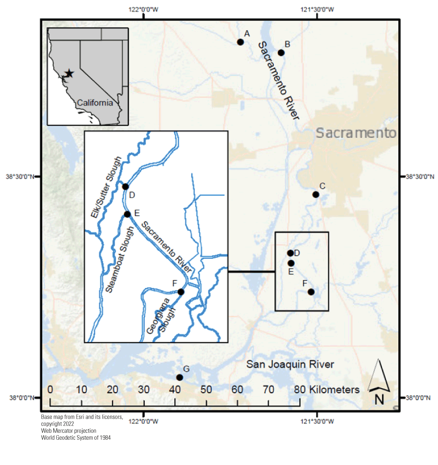
Sacramento-San Joaquin River Delta system. Map shows (A) Knights Landing, the rough location where observed catch data was collected; (B) Verona, California, the salmon (Oncorhynchus spp.) routing time and travel simulation (STARS) simulated fish release location; (C) Freeport gauging station, the primary gauging station used in simulations; (D) Sutter Slough junction, (E) Steamboat Slough junction, (F) Georgiana Slough junction and (G) Chips Island, the end of STARS simulated passage and point of assessed through-delta survival.
Survival outcomes can significantly differ between routes and flows due to differences in the distances traveled, predation rates, and exchange into the interior Sacramento-San Joaquin River Delta (Perry and others, 2013). For example, survival of juvenile salmon in the slough channels is lower than in the Sacramento River at low flows. Whereas survival in the slough channels is similar to survival in the Sacramento River at flows above about 35,000–49,000 cubic feet per second (ft3/s; Perry and others, 2018). Through-delta survival of juvenile salmon increases with flow, partially because higher flows result in lower entrainment into the interior Sacramento-San Joaquin River Delta where survival is low (Perry and others, 2015, 2018). Sacramento River flows are also positively related to survival within Steamboat and Sutter sloughs, the Sacramento River between Georgiana Slough and Rio Vista, and in Georgiana Slough (Perry and others, 2018).
To increase the number of fish traveling through routes that result in high survival of out-migrating salmonids through the Sacramento-San Joaquin River Delta, the California Department of Water Resources (DWR) began experimenting with the use of fish guidance structures (hereinafter referred to as behavioral barriers) in 2011. A BAFF that included sound, light, and bubbles to deter fish was experimentally deployed at the Georgiana Slough junction with the Sacramento River in 2011 and 2012 (California Department of Water Resources [DWR], 2012, 2015). This BAFF reduced entrainment into Georgiana Slough by an average of 14.6 percent (Perry and others, 2012). A FFGS was experimentally deployed just upstream of Georgiana Slough in 2014 (Hance and others, 2020). This FFGS reduced entrainment by about 5 percent when flows were no more than about 14,000 ft3/s (Romine and others, 2016). However, overall through-delta survival was not improved by the presence of the FFGS at Georgiana Slough (DWR, 2016). Given the reduction in entrainment, and to meet the 2020 California Department of Fish and Wildlife’s (CDFW) Incidental Take Permit (ITP) Minimization Measure 8.9.1, the DWR plans to install the Georgiana Slough salmonid migratory barrier (GSSMB) from the spring of 2023 until 2030 (CDFW, 2020). Because the effectiveness of these behavioral barriers depends on shape, length, position, and type of barrier, there is a need to determine what designs might maximize through-delta survival.
We developed the BOT to optimize the design of future barriers. This tool addresses the 2020 CDFW ITP Minimization Measure 8.9.2 (CDFW, 2020) to evaluate guidance barriers at the junctions of the Sacramento River at Steamboat Slough and Sutter Slough. The BOT allows investigators to efficiently evaluate how barrier type, orientation, and length could affect entrainment and survival without the need for numerous, repeated, time consuming, and costly field trials. We demonstrate the use of the tool to design behavioral barriers at the Steamboat Slough and (or) Georgiana Slough junctions within the Sacramento River given two proposed operational time periods. This tool allows managers to evaluate and update barrier designs in response to flow and operational timing as additional data are collected.
Barrier Optimization Tool Overview
The BOT uses machine learning approaches inspired by the process of natural selection known as genetic algorithms to iteratively create, test, and evaluate possible barrier designs (Yu and Gen, 2010; fig. 2). Genetic algorithms start by testing hypothesized solutions to a problem. At the end of the first test, solutions undergo a reproductive process inspired by biological processes in which the solutions that return better results are given greater weight. Through many iterations of testing and reproduction, potentially better solutions evolve.
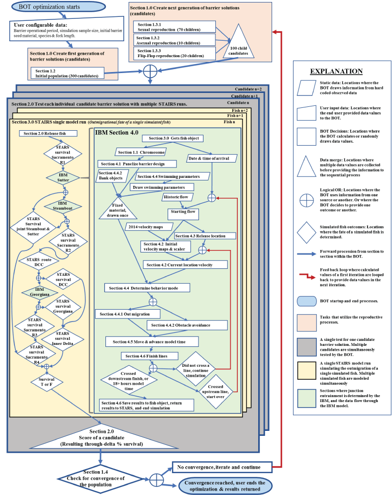
Flow chart showing the barrier optimization tool processes. The chart shows processes as described in sections 1.0–4.0 of this report. The flow chart starts with the three steps in creating a generation of barrier solutions. It then shows how candidate solutions are tested within multiple salmon, travel time, and individual routing simulation (STAIRS). A flow chart showing how fish routing is simulated past Steamboat and Sutter sloughs and the delta cross channel (DCC) is displayed. Routing decision points within the salmon, travel time, and routing simulation (STARS) are highlighted in green and indicate the location where the individual based model (IBM) was inserted into the model. Details about how the IBM works, as described in sections 3.0 and 4.0 of this report, are shown as a flow chart.
We programed the BOT using the LabVIEW programming software (Blume, 2017) to evolve and design a combination of fish behavioral guidance structures at Sutter, Steamboat, and Georgiana Slough junctions with the Sacramento River into a single possible candidate barrier solution (henceforth referred to as a candidate). In our demonstration of this tool, we used a combination of previously used barrier designs and hypothesized design solutions to seed the model with initial candidates. To test each candidate, the BOT simulates through-delta passage of juvenile fish that carry a candidate with them. The BOT then scores the candidates by how many simulated fish survive given the candidate barrier design combination. The scored candidates undergo a machine learning approach that mimics biological reproductive processes to create a new population of candidates different from the first. The BOT is manually stopped when the current generation of candidates have converged on a specific set of traits that result in similar scores and share very similar barrier designs at all three junctions.
Routing entrainment and survival of juvenile Chinook salmon (Oncorhynchus tshawytscha) though the Sacramento-San Joaquin River Delta are simulated using a modified version of the STARS model (Perry and others, 2019). STARS models through-delta survival of a cohort of fish using a series of junction specific routing probabilities and reach specific survival from Verona, California, below the confluence of the Feather River and Sacramento River, through Chipps Island, California. The probabilistic routing at the three junctions of interest within STARS were replaced in the BOT with an IBM so that the effects of barrier implementations could be considered. The combination of these two models is called the salmon travel time and individual routing simulation (STAIRS) model.
The IBM uses a passive particle tracking approach modified to include fish swimming behavior to track fish through a junction until a route is determined. Modeled swimming behaviors include cross-stream and along-stream movement, and rheotaxis behavior. The simulated fish responds to objects such as banks and barriers in accordance with previously observed response distances. The barrier configuration modeled in each individual IBM trial is determined by the candidate carried by the simulated fish. When a simulated fish crosses a downstream finish line, and thus the route is determined, the IBM model stops and passes the fish back to STARS so that the simulated fish can continue its outmigration.
1.0. The Genetic Algorithm
We used a genetic algorithm to test thousands of possible barrier designs. A genetic algorithm is a metaheuristic mathematical approach used in some machine learning models that mimics the process of natural selection of the fittest candidates (Mirjalili and others, 2020). Genetic algorithms begin with a starting population of possible solutions. In our implementation, the information defining a candidate’s unique barrier designs is contained in a data structure called a chromosome. To initiate the genetic algorithm, an initial population of candidates are created by the user and are tested and scored using STAIRS. Then a new generation of candidates are produced using reproductive processes where candidates with the better scores are weighted more favorably. For each iteration of the genetic algorithm numerous copies of each unique chromosome are tested. This process is iterated until the variation within the current population of candidates is minimal and begins to reach a state of convergence (see “1.4 Population Convergence”).
1.1. Chromosome Design
Chromosomes contain the details describing a set of barrier designs including the barrier types at each junction, coordinate for the barriers’ starting locations, and include information that defines the exact location of the barrier (fig. 3). The chromosome is stacked into three sequential sections, one each for Sutter, Steamboat, and Georgiana sloughs (fig. 4). Each section contains all the specific information needed to model the effects of a barrier at each junction. Each section is made up of a one-dimensional array where the first array element is an integer of either 0, 1, or 2 that determines the barrier type: no barrier, BAFF, or FFGS, respectively. The second array element is an index to a lookup table that provides the starting coordinates of the barrier. We laid out start locations along lines that were 1 meter (m) apart and set perpendicular to the bank. Although the chromosome structure allowed for evaluation of barriers at Sutter Slough, at the time of these optimization efforts Sutter Slough was not included as a primary focus in the Minimization Measure 8.9.2 (CDFW, 2020). Therefore, in our implementation of the BOT no barriers were modeled as Sutter Slough. Instead, the IBM modeled fish at Sutter Slough in the absence of a barrier.
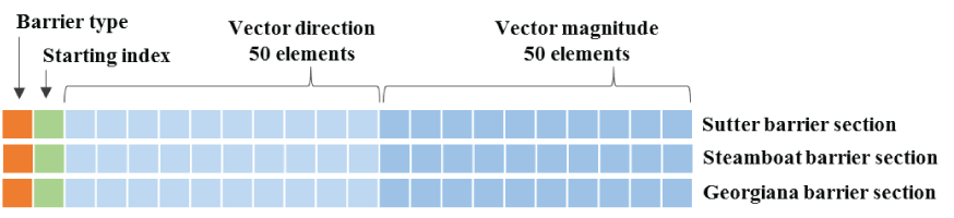
Genetic algorithm’s chromosome design that contains information of a candidate barrier solution used to create a single barrier design at each of the three junctions. The diagram shows three example vectors, one for each junction, Sutter, Steamboat and Georgiana sloughs. Each example data vector is composed of a one-dimensional numeric array that defines the type of barrier, the starting location of the barrier, and 2 sets of 50 sequential vectors that indicate the vector direction and magnitude.
The process for sexual reproduction of the genetic algorithm’s chromosomes. The sexual reproduction method that uses two parent chromosomes selected from a mating pool model to create a child candidate barrier solution with unique new barrier designs for each junction, with shared traits of the selected parents. The diagram shows two example data vectors, one for each parent. Each example data vector is composed of a one-dimensional numeric array that defines the type of barrier, the starting location of the barrier, and 2 sets of 50 sequential vectors that indicate the vector direction and magnitude. The letters F and X on the vectors indicate which parent contributes each element of data to the resulting child vector.
The remaining 100 array elements are used to describe 50 sequential vectors. Each vector was described by two array elements, a direction in decimal degrees and a length. The first vector starts at the barrier’s indexed starting location. The end of the first vector defines the starting location of the second vector, and the second defines the starting location of the third, and so on until all 50 vectors are sequentially described. The 51 coordinate sets of the intersections and starting index are used in later processes to create an unbounded spline. The spline is used in a panelizing routine to construct a practical discretized version of the barrier shape that is evaluated through the IBM.
1.2. Creating an Initial Population of Candidates
In our implementation of the BOT we seeded the genetic algorithm with eight barrier designs for Steamboat Slough, and six barrier designs for Georgiana Slough. These initially hypothesized barrier designs were put through a reproductive process modeled after sexual reproduction (see “1.3.1 Sexual Reproduction with Mutation”) to create 300 unique candidates that made up the first generation tested in the genetic algorithm (figs. 5, 6). Given that there has not been a barrier study performed at Steamboat Slough, the hypothesized barrier designs were based on the professional judgment of a team of Sacramento River Chinook entrainment experts. Two of these designs were aimed at decreasing entrainment, while the other six were aimed at increasing entrainment (fig. 5). This was done because entrainment into Steamboat Slough can either increase or decrease through-delta juvenile salmon survival, depending on water velocity and downstream entrainment rates. The hypothesized barrier designs varied in length, angles, and curvature. The initially hypothesized barrier designs at Georgiana Slough included (1) the barrier location used during the 2011 and 2012 BAFF studies (DWR, 2012, 2015), (2) the 2014 FFGS barrier location (DWR, 2016), (3) three barriers that resembled the 2011 BAFF but were extended further around into the Sacramento River with varying levels of curvature at each end, and (4) a shortened barrier pushed farther into Georgiana Slough (fig. 6).
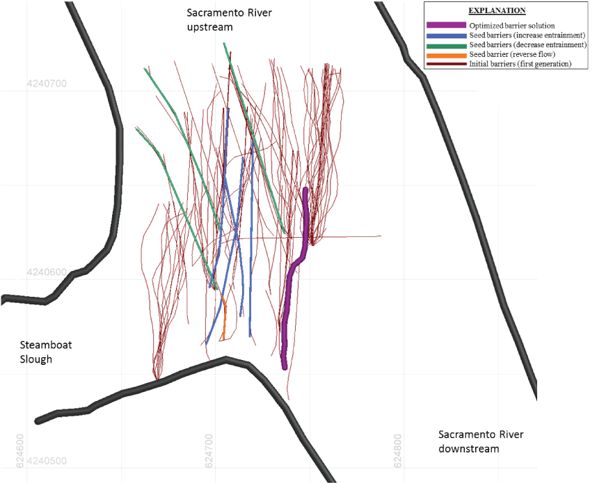
The relationship between the seeding barrier designs, and a resulting possibility for the initial population of barrier candidates at Steamboat Slough. This example was taken from an optimization effort in which barriers were considered at Steamboat and Georgiana sloughs from November 1 to March 15. It shows the Steamboat Slough initial seeding barrier designs intended to increase entrainment, seeding barrier designs intended to decrease entrainment, and a seeding barrier design with the intent of decreasing entrainment during tidally driven flow reversal. The initial population of candidate barrier solutions created from the seeding barriers (in other words, first generation) are shown in grey, and the resulting optimized barrier solution is shown.
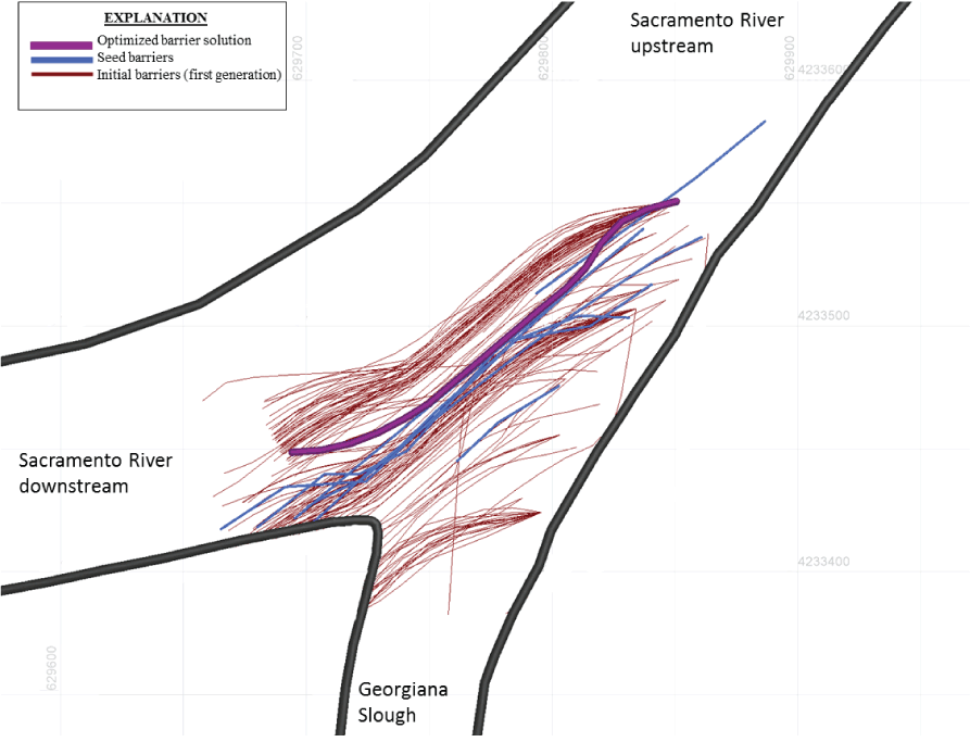
The relationship between the seeding barrier designs, and a resulting possibility for the initial population of barrier candidates at Georgiana Slough. This example was taken from an optimization effort in which barriers were considered at Steamboat and Georgiana sloughs from November 1 to March 15. The Georgiana Slough initial seeding barrier designs intended to decrease entrainment, the initial population of candidate barrier solutions created from the seeding barriers (in other words, the first generation), and the resulting best barrier solution are shown.
1.3. Reproduction
In each iteration the BOT genetic algorithm uses three reproductive methods to create new candidates (children) to be tested. These children represent a new generation of potentially better barrier solutions. We coded three reproductive methods to create these children: sexual, asexual, and flip-flop reproduction. Each of these reproductive methods is configured to allow the BOT to explore varying degrees of change in barrier designs. For the first generation all 300 candidates are created using sexual reproduction from the seeding material. All subsequent iterations create 100 children candidates. Seventy of the children are created through sexual reproduction to explore the greatest potential in diverse designs. Ten children are created from asexual reproduction to explore subtle variations among designs. Twenty are created from a flip-flop procedure that ensures that a single junction’s barrier is not driving inefficient barrier designs at the other junction. The number of children were chosen through trial and error to balance the computational time with the number of potential solutions.
During the reproductive cycle in every iteration of the BOT, a mating pool of available candidates for reproduction is created. The mating pool is composed of either the 300 candidates when creating the second generation, or the 100 recently tested candidates of a generation for every preceding iteration of the BOT. Except for the first generation, every other generation has the highest scoring candidate from any previous generation added to the mating pool of 100 individuals to ensure that the best result so far is thoroughly explored. Additionally, the initially hypothesized six Georgiana barriers and the eight Steamboat barriers that created the seeding candidates are treated as fixed material and added back into the mating pool in every generation other than the first. By adding these barrier designs back into the mating pool we were ensuring a robust evaluation of these specific designs. This also helped to ensure that the resulting barrier designs could realistically be constructed.
1.3.1. Sexual Reproduction with Mutation
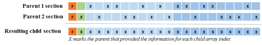
After the mating pool is established, the reproduction process starts by creating 70 children through sexual reproduction. First the mating pool is randomly divided in half to create two pools of parents. From each parent pool, 30 candidates are randomly selected. From these two pools of 30 potential parents, the candidate with the highest score is selected as the parent. After the two parents are selected, sexual reproduction starts by indexing out the individual sections (Sutter, Steamboat, and Georgiana) from the chromosome from each parent. Then for each section starting at the first array element within that section a value is selected randomly from either of the parents. This process is repeated for all 102 array elements. The three new sections representing a barrier design at each junction are sequenced together to create the chromosome for the resulting child (fig. 7).
The resulting child chromosome is then mutated by randomly modifying the elements within the chromosome. For sexual reproduction, mutations were implemented by converting each integer within the one-dimensional array of each section of the chromosome into a bit array. A bit array is a data structure represented by series of simple two state choices. These integer values were converted into a 64-element bit array. The proceeding elements of the bit array determine the sequence of digits of the integer value starting with the least significant digit first. Therefore, changes to the first couple of bits will change the smallest digits within the integer value. The mutation is performed by randomly flipping the state of individual bit elements within the bit array. Making changes farther along the bit array will cause greater changes in barrier design (fig. 7). The first array element in each section of a chromosome represents the barrier type and can be exempted from mutation if the user wants to fix the barrier types at each junction. To explore a wide range of potential solutions, mutation parameters were set to encourage aggressive mutation for sexually reproduced children, therefore the second array element that is the starting index which anchors the barrier start location was allowed to mutate no greater than 72 integers (fig. 7). The vector components used in the panelizing routine were limited to mutations no greater than 72 degrees (°), and 72 m (see “4.1 Panelizing a Barrier”).
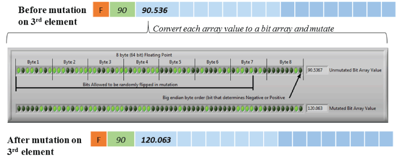
Sexual mutation method in the genetic algorithm applied to a child chromosome. Below is a diagram showing how one element in the chromosome is converted to a 64-bit array, and how random mutation is applied to elements within the bit array. Then an example of the new mutated bit array is shown. Each array element within a section is converted into a bit array where each bit within a defined portion of the array then has a randomizing routine applied to possibly swap the bit state. The array elements of the bit array allowed to be swapped are defined to limit the mutation within acceptable tolerances. This mutation method can result in subtle or extreme changes within the barrier designs. The bit array mutation allowed values to be modify up to roughly plus or minus (±) 72 integers.
1.3.2. Asexual Reproduction
Asexual reproduction explores the effects on performance through subtle changes in high performing candidates. Asexual reproduction starts by selecting the 10 highest scoring candidates within the mating pool. Each of the 10 selected candidates are mutated by adding or subtracting a value randomly selected from within a user specified range to each array element. For the BOT examples explored in this report, the first array element that defined barrier type was not allowed to mutate. The second array element for the starting index was set to change by as much as five indices, which anchors the starting location of the barrier. The vector components could change as much as 5° and 5 m.
1.3.3. Flip-Flop Reproduction
The performance of a candidate depends on the effects of barrier designs at multiple junctions. A candidate with a high performing barrier design at one junction may overpower the effects of a low performing barrier design at another junction. The synchronized evolution of barriers at multiple junctions could lead to false conclusions when the performance of a barrier design for one junction is considered independently. To ensure that less effective barriers at one junction are not arbitrarily scored high by being linked to more effective barriers at the other junction, we used flip-flop reproduction. Instead of modifying barrier characteristics, flip-flop reproduction swaps the sections describing barriers at individual junctions with those of another chromosome to create new combinations of barriers.
Flip-flop starts by randomly dividing the mating pool in half and selecting 30 candidates at random from each half. Then the highest score from each group of 30 is selected as the parents. Then each of the sections (Sutter, Steamboat, and Georgiana) are selected at random from one of the parent chromosomes to create the child. This is repeated 20 times, using 20 sets of parents, to create 20 flip-flop children (fig. 8).
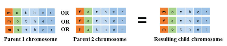
Flip-flop mutation used in the genetic algorithm. Flip-flop mutation swaps entire sections of the chromosome randomly selected from one of two parent chromosomes. The resulting child has the exact same barrier design as one of its parents, where each barrier design for a junction may have come from either parent. The diagram shows chromosomes for each of two parents. Each chromosome is made up of three vectors, one each for three junctions within the Sacramento-San Joaquin River Delta. When these are combined the resulting child has vectors from both parent chromosomes.
1.4. Population Convergence
The BOT was written to ensure there would always be variance within the population, and it will never fully converge on a single solution. Because of this, it is difficult to program in a convergence trigger to end the genetic algorithm. Instead, the BOT was manually ended by a user when roughly 85 percent of the barriers represented on a graphical interface were nearly identical in size, shape, and location. Geographically this equated to the dominant solutions converging roughly within about 5 m along the length of the barriers and within roughly 20 m in overall length.
2.0. Testing and Scoring Candidate Barrier Solutions
To test each candidate, each of the 300 (first generation) or 100 (all subsequent generations) candidates were attached to 15,000 simulated winter-run-sized (155 mm) Chinook salmon in each model iteration. These were distributed as 1,000 simulated fish per candidate per model iteration per simulated year. This resulted in 4,500,000 through-delta fish simulations in the first generation and 1,500,000 in each subsequent generation. When each simulated fish entered a junction, it provided the appropriate section of the chromosome to the IBM so that the effects of that candidate’s barrier designs could be tested on the simulated fish. Candidates were scored based on the portion of fish tested using their barrier design that survived the through-delta journey.
2.1. Fish Object Data Structure
Fish were simulated using a data structure called a fish object that contains all the necessary information to model the outmigration of a simulated fish within the BOT. The fish object contains an assigned candidate, barrier operational period, starting date and time of the fish simulation based on the observed fish distribution data, and the barrier cost constraint information. As the fish passes through the simulation, the fish object collects information on reach travel times, entrainment outcomes, and mortality state (in other words, alive, dead, or error). When a route within the IBM cannot be determined within 18 hours, a mortality state of error is recorded, and the fish is censored from the survival score. Fish in a dead or error state cease to propagate through the STAIRS model.
2.2. Timing Simulated Fish Released to Real World Observations
To represent real-world fish distributions across a range of real-world discharges we simulated passage of 1,000 fish in each of 15 years. The simulated fish were distributed among days of the year using the observed daily proportional catch per unit effort data for winter-run-sized Chinook salmon collected at Knights Landing (Columbia Basin Research, 2022). Run classifications were performed by California Department of Fish and Wildlife (CDFW) based on length-at-date assignments (Harvey, 2011). Release time is simulated to occur at random throughout each 24-hour period. At the time simulations were being run, these data were limited to 1997–2011 because these were the only years that were processed and proofed by run classification assignments (fall, winter, spring, and late-fall Chinook salmon).
3.0. Integration of Models
To test the effects of a candidate on entrainment rates, we replaced the probabilistic STARS-calculated entrainment rates at Sutter, Steamboat, and Georgiana sloughs with an IBM. Because Sutter and Steamboat sloughs are only about 2.4 kilometers (km) apart, STARS does not calculate the survival reach between the two junctions. Instead, STARS uses a three-way routing probability to determine fish entrainment between Sutter, Steamboat, and the Sacramento River. We replaced the three-way probabilistic route determination of STARS with the IBM for each of these junctions. Given that STARS does not consider the travel time in the reach between Sutter and Steamboat sloughs, we added an additional length of river to the Sacramento River passage route at the downstream end of Sutter Slough the same length as the real distance between these junctions (figs. 9, 10). This timing reach ensured accurate arrival timing at Steamboat Slough. Both STARS and STAIRS assumes no mortality occurs between Sutter and Steamboat sloughs.
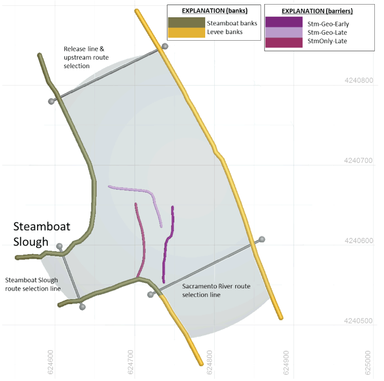
Steamboat Slough bank avoidance terms as applied to individual portions of the riverbanks. The three bold barrier designs are the resulting optimized barrier solutions for the three optimization simulations (table 1). The shaded area represents the slow timing zone area and unshaded areas are fast timing zones. Grid spacing is in UTM Zone 10 Cartesian coordinate system.
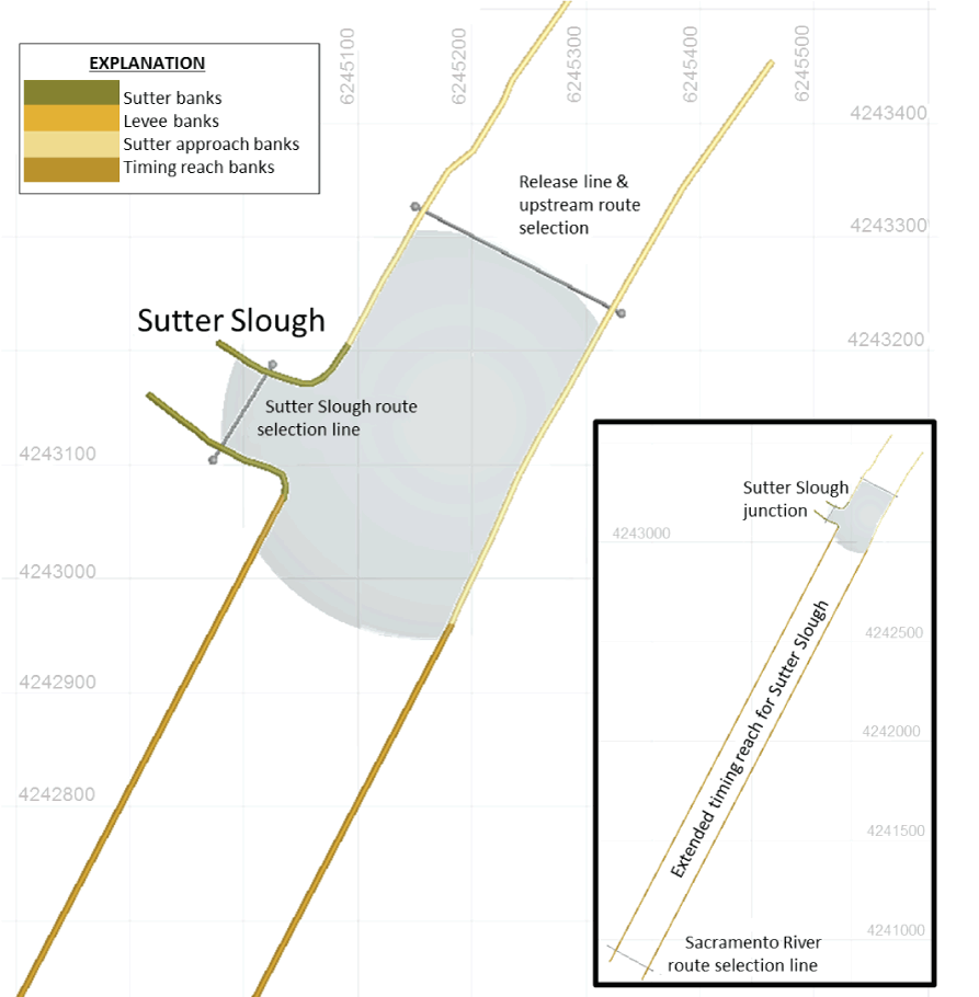
Sutter Slough bank avoidance terms as applied to individual portions of the riverbanks. The diagram shows the bank avoidance terms as applied to individual portions of the riverbanks at Sutter Slough (table 1). The length of the extended timing reach used to account for travel time between Sutter and Steamboat sloughs is also shown. The shaded area represents the slow timing zone area and unshaded areas are fast timing zones. Grid spacing is in UTM Zone 10 Cartesian coordinate system.
When Sacramento River flows at Freeport are below approximately 18,000 ft3/s, the flow in the Sacramento River at the Georgiana Slough junction can reverse on incoming tides. Moreover, there are periods when the entirety of the Sacramento River flows into Georgiana Slough (DWR, 2016). Flow reversal increases entrainment into Georgiana Slough (Perry and others, 2015). Fish that are routed down the Sacramento River past Georgiana Slough can still be entrained in Georgiana Slough if they are not far enough downriver before tidally driven flow reversal occurs. Fish that are transported back upstream into the junction are exposed to an additional and different entrainment risk as they move through the junction. To account for the effect of reversing tidal currents, the IBM includes an extended length of river we call a timing reach that extended roughly 550 m downstream in the Sacramento River from the Georgiana junction (fig. 10). This extended timing reach allowed fish to move back and forth during changing tidal conditions until they are fully committed to either Georgiana Slough or the Sacramento River. A similar approach was not taken at Steamboat and Sutter sloughs because flow reversal in the Sacramento River only occurs in these junctions under very low flow and is uncommon.
4.0. The Individual Based Model
The IBM simulates the movement and entrainment of individual juvenile salmon as they pass each junction. The IBM adds swimming behavior to passive particle tracking within a two-dimensional surface water velocity map to simulate the overall movement of fish through junctions. The swimming behavioral parameters include an avoidance component that allows a simulated fish to actively swim and respond to banks and barriers. The IBM spatial framework uses the Universal Transverse Mercator (UTM) zone 10 north coordinate system.
The IBM is initiated when a simulated fish enters one of the three junctions of interest. The IBM contains static data on bank locations, and it retrieves information about the barrier from the Fish Object (see “2.1 Fish Object Data Structure”). This includes the barrier operational period, the barrier cost constraints that limit the barrier designs, and the section of the chromosome that contains barrier design data. The IBM then performs a panelizing operation to create the barrier that the individual simulated fish may encounter (see “4.1 Panelizing a Barrier”). If the simulated fish arrives at a junction outside of the barrier operational period, its passage through the junction is modeled in the absence of a barrier. A river flow value is selected from a table of observed data based on the simulated fish’s arrival time at the junction (California Data Exchange Center, 2022; U.S. Geological Survey, 2023; National Water Information Site number 11447650). This value is used to select a starting water velocity map (see “4.2 Water Velocity Mapping”) and a release location of the simulated fish along a start line perpendicular to the river upstream of the junction (see “4.3 the Release Line”). The IBM then randomly draws unique swimming parameters that are applied to the simulated fish (see “4.4 Applying Swimming Parameters”).
Simulated fish locations are iteratively updated using the vector addition of the fish’s movement in response to water velocity and swimming behavior at each model interval (t; see “4.6 Advancing Model Time and Location”) until the fish crosses a downstream finish line, upstream start line, or until 18 model hours have passed. Fish movement considers the swimming parameters drawn at the start of the IBM and the fish behavior relative to the proximity of banks and barriers (see “4.5 Behavior Modes and Movement”). When simulated fish cross the upstream start line the IBM starts over, using the time that a fish exited the area as the new start time. In these incidents the fish continues to use the initial swimming parameters drawn when it entered the junction.
4.1. Panelizing a Barrier
The vectors stored in the chromosome describe a barrier of an unrestricted length having panels of nonuniform length. However, in the real-world cost restricts the total length of barriers and barrier panels have a fixed length. Therefore, to convert the design information stored in the appropriate section of the chromosome into a realistic barrier design, a panelizing routine was programed into the IBM (fig. 11). First, the IBM calculates the coordinates at the beginning of each of the 51 vectors based on data in the chromosome. Then, the IBM fits an unbounded spline through these 51 points. This spline does not define the barrier location, only the path on which to construct the barrier. The panelizing routine then references the cost components that set the panel size of each barrier type and the maximum number of panels a barrier type can have. The IBM fits up to the maximum number of fixed-length panels, as determined by the cost component for each barrier type, to the spline. The resulting series of panels define the barrier shapes that were evaluated in the IBM.
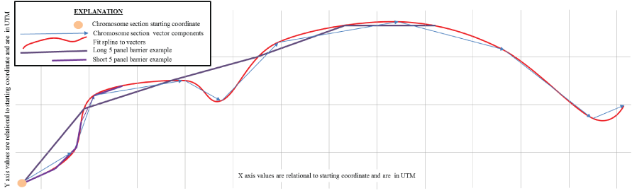
Panelizing process by which vector components in the chromosome are translated into barrier objects. The two examples of barrier designs shown here both used five panels within their cost component, but have different lengths assigned to them. Lengths of panels and thus cost components are dependent upon the type of barrier bioacoustics fish fence or floating fish guidance structure.
The size and maximum quantity of panels can be defined by the user, which was fixed to match previously constructed barriers. For BAFF type barriers, we fixed the panel length at 12 m and a maximum of 16 panels. This allows for a maximum BAFF barrier length of 192 m. For FFGS type barriers the panel length was set to 6 m and the maximum number of panels was 16, for a total length of 96 m. These cost components prevent the BOT from creating unreasonably long barriers and restrict project costs such that they would be similar to past projects.
4.2. Water Velocity Mapping
The IBM was developed specifically to operate using surface water velocity maps that were generated from interpolating acoustic Doppler current profiler (ADCP) and horizontal ADCP (HADCP) data collected during the 2014 FFGS study at the Sutter, Steamboat, and Georgiana slough junctions. These velocity maps were interpolated to a spatial resolution of 10 m and temporal resolution of 15 minutes over roughly a 3-month period (DWR, 2016). The maps were limited to the immediate junction region and do not extend into the vicinity of the banks. They were only collected during the spring of 2014 and covered Sacramento flows between roughly 5,000 and 30,000 ft3/s, which were lower flows than were typical during the full period of record (fig. 12). As a result, a water velocity interpolation and extrapolation scheme was developed so that water velocities over the complete simulation period could be estimated at every t.
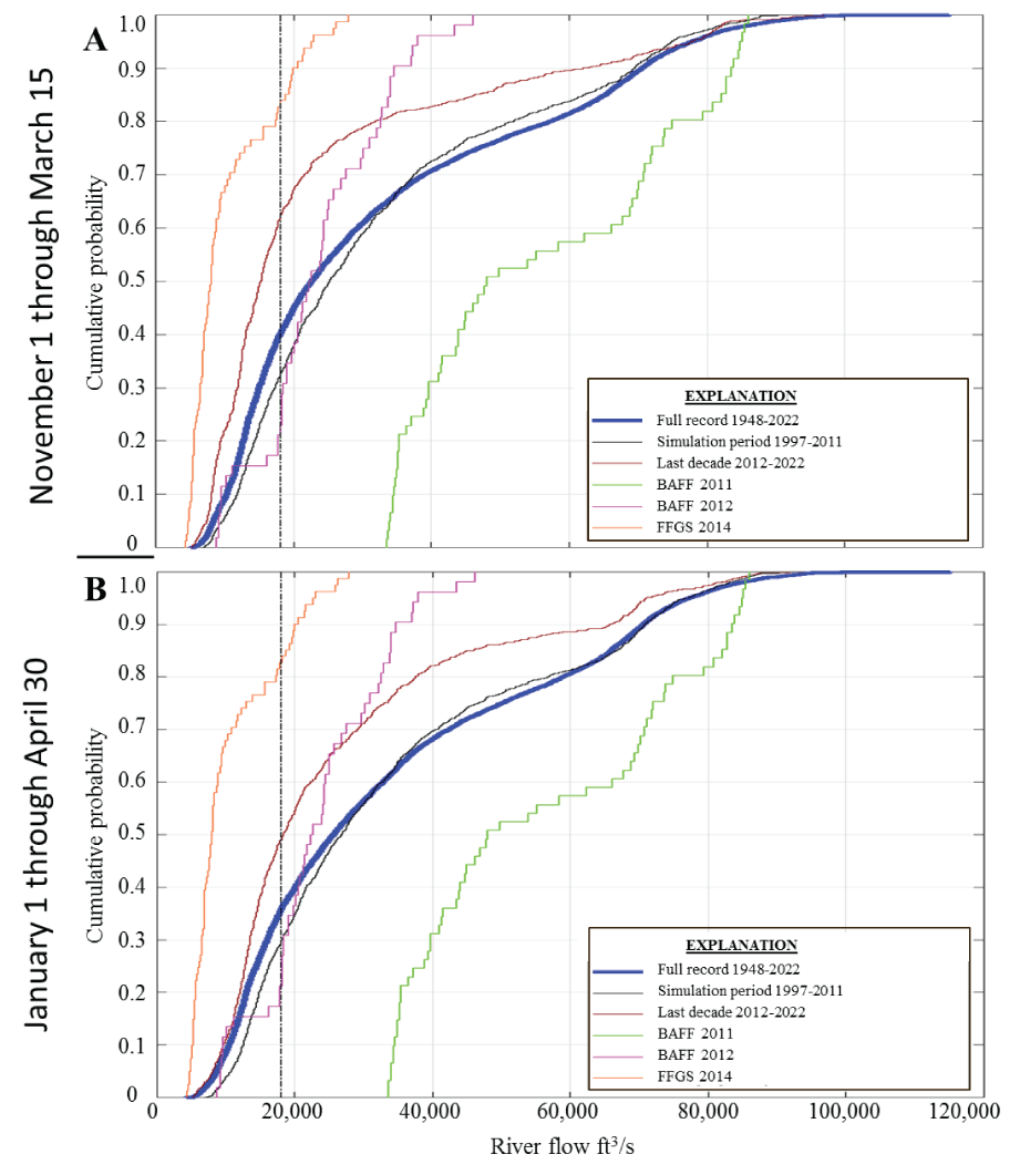
Cumulative distributive function for Sacramento River flows at Freeport, California. The cumulative distributive function for Sacramento River flows at Freeport, California (National Water Information System site 11447650) over early (A) and late (B) operational periods considered in the barrier optimization tool is shown. These plots show the cumulative probability that a given flow value or less was experienced within each block of time. The vertical dashed line denotes river flows of 18,000 cubic feet per second (ft3/s). River flows under about 18,000 ft3/s are subject to tidally forced flow reversals at Georgiana Slough.
This process starts by identifying the closest 2014 velocity map to the flow corresponding to the simulated fish’s arrival time. First the IBM uses historical gage data to estimate the 15-minute average flow entering the junction (Qa) and exiting the junction in one of the downstream branches (Qb). It then compares the weighted inverse distance of the arrival time ([Qa, Qb]T) to the [Qa, Qb] values for each 15 minute velocity map from the 2014 data to find the 2014 water velocity map that is closest to the simulated time.
Given that during the simulation period used in the BOT river flows were greater than those mapped in 2014, a routine was developed to extrapolate water velocity maps for conditions higher than those observed in the 2014 study. When Qa is greater than the data collected in 2014, the closest 2014 velocity map is selected, and a scaling factor (Sv) is applied. This method is valid because as mean Sacramento River flow increases, the strength of tidal forcing decreases to the point where the 2-dimensional velocity distribution in a junction stabilizes (DWR, 2016).
We calculated a scaling factor (Sv) by applying a best fit third order polynomial to the cross-sectionally averaged velocity as a function of river discharge for discharges above which the velocities in a given junction became non-tidally affected. For the Sutter Slough and Steamboat Slough junctions, SV was estimated based on flow data collected at the Freeport gauge between 2011 and 2019 (National Water Information System, site 11447650). At Sutter and Steamboat junctions, velocities were considered non-tidally affected when variations at spring/neap (fortnightly) timescales in the discharge ratio cease to exist, which occurs at Freeport flows at about 29,000 ft3/s. In the simulation, the BOT estimates the velocity at the Sutter Slough and Steamboat Slough junctions by multiplying the observed discharge at Freeport for the current model time by Sv (fig. 13). Similarly, SV at the Georgiana Slough junction was estimated by fitting a third order polynomial to the cross-sectionally averaged velocity at the Sacramento River above the Delta Cross Channel site (U.S. Geological Survey National Water Information System, site 11447890) using data from 1996 to 2011 during non-reversing periods that occur above Freeport flows of about 18,000 ft3/s (fig. 14).
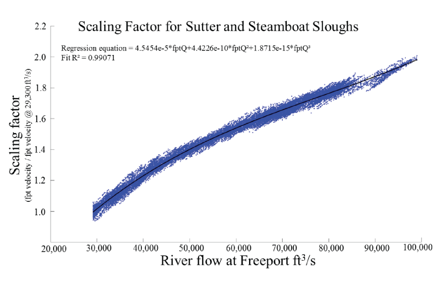
Water velocity scaling factor for Sutter and Steamboat sloughs applied when river flow values at Freeport, California exceed 29,300 cubic feet per second (ft3/s). Data are from the U.S. Geological Survey National Water Information System, site 11447650. Flow values were collected between 2011–19.
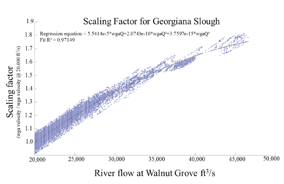
Water velocity scaling factor for Georgiana Slough applied when river flow values at Walnut Grove, California (U.S. Geological Survey National Water Information System, site 11447850) exceed 18,000 cubic feet per second (ft3/s). Flow values were collected between 1996–2011.
The IBM interpolates and scales a water velocity map at each model time t. This process starts by using the first 2014 velocity map identified from the [Qa, Qb] relationship. The IBM then indexes the next sequential 2014 map and applies a time weighted average interpolation between the maps. As the model iterates, the IBM continuously interpolates a new water velocity flow field from the 2014 15-minute velocity maps proportionally weighted towards either the previous or next sequential map based on how much model time has elapsed since time t when the previous map was first indexed. Then the water velocity flow field is scaled by Sv.
Because the 2014 water velocity maps did not measure velocities near the shorelines, they do not account for decreasing velocities near the banks. To correct for this, the classic log law was applied using factor (St) (Chow, 1959) to scale the water velocities toward zero near the bank boundaries. St is a manually calibrated term, constant for all bank objects, and is applied starting at 6 m from the bank. This ensures that as simulated fish approach a bank, they experience a diminishing velocity that will not allow them to be advected through the bank.
4.3. The Release Line
Simulated fish are released into the IBM along starting lines perpendicular to the Sacramento River roughly 300 m upstream of each junction. The entrainment rate in any junction is a function of the cross-stream distribution of the fish as they enter a junction. We assigned positions along release lines using a random weighted draw from observed flow dependent cross-sectional fish distributions when adequate data were available (DWR, 2016). These data are sparse at Sutter Slough, and unavailable at Steamboat Slough. To calibrate the distribution of starting locations along the release lines at these two junctions we developed a calibration routine that simulated random fish releases into the junctions at different river flows and calculated the resulting entrainment rates (see “4.8 IBM Model Calibration”).
4.4. Applying Swimming Parameters
Simulated fish are assigned a set of swimming parameters at the beginning of the IBM. These parameters dictate the cross-stream swimming speed and rheotaxis behavior that are assigned from an array of parameters that were calculated from over 2,500 unique fish tracks collected during the 2014 FFGS barrier study (DWR, 2016). To calculate a set of swimming parameters, a passive particle was released into the velocity field at each location of the observed fish track. The swimming efforts were deduced by subtracting the passive particle trajectory from the observed fish tracks over the same time interval.
At the start of every IBM for each simulated fish, three parameters calculated from a single observed fish track were randomly chosen. Swimming parameters include the mean (XSm) and standard deviation (XSstd) of the cross-stream swimming velocity and the mean along-stream swimming velocity (ASm). These swimming parameters stay with the fish throughout the simulation in a single junction but are not attached to the fish object and therefore do not follow to subsequent junctions. The cross-stream velocity of the fish was calculated as the velocity normal (90°) to the particle movement. Swimming velocity directly in line with water velocity is the along stream swimming velocity ASm. These values are calculated as the mean of the along-stream difference in velocity from the tangential accelerations of all the differences of the passive particle and observed fish movements. Negative ASm values correspond to positive rheotaxis movements or actively swimming against the flow. Positive ASm values correspond to negative rheotaxis efforts or actively swimming with the flow.
The swimming simulation starts by randomly drawing a new cross-stream swimming velocity (XSu) from a normal distribution with a mean of XSm and a standard deviation of XSstd. The beginning direction of a simulated fish’s cross-stream movement in each IBM model interval is randomly selected. XSu is applied normal to the water velocity in the same orientation during a single cross-stream transect. This means that the selected XSu value will continuously move the simulated fish across the river current toward either the right or left bank until some stimuli forces a change in direction. Changes in direction are simulated by adjusting the vector normal by 180° so that the next movement in the next t is in the opposite cross-stream direction. XSu is drawn at the beginning of every new cross-stream transect. The sum of ASm and XSu equals the swimming velocity of a simulated fish at t regardless of their location within the water velocity flow field.
4.5. Behavior Modes and Movement
Simulated fish act in one of two behavioral modes: out-migration or obstacle avoidance. Out-migrating fish exhibit high velocity seeking behavior. Whereas, in obstacle avoidance mode fish respond to banks and barriers. Simulated fish can only exhibit one behavior at a time. The behavioral mode is determined at the beginning of each IBM model interval t based on the fish’s distance from banks and barriers. Simulated fish exhibit the out-migration behavioral mode until they get within a defined response distance of a bank or barrier, at which point they enter the obstacle avoidance behavior mode. The fish remains in obstacle avoidance mode until no obstacles are within the defined response distances.
4.5.1. Out-Migration Behavior
Out-migration behavior is based on analysis of juvenile winter-run-sized Chinook salmon tracks collected during the 2008 North-Delta study and the 2014 FFGS study that showed many fish exhibited consistent periodic cross-stream movement (Holbrook and others, 2009; Romine and others, 2016; DWR, 2016). This cross-stream movement becomes more prevalent as water velocities decrease. It is hypothesized that juvenile salmon swim at approximately 45 degrees to the water current, which provides an energy efficient way to move across the river. This behavior would allow the fish to assess the velocity field while possibly seeking high water velocity to maximize out-migration speed. It may also help fish to find within channel and near bank velocity refugia, or suitable littoral habitat (for example, not rock) or to avoid near bank predators (DWR, 2016).
To simulate a similar cross-stream out-migration behavior we programed simulated fish to change their cross-stream direction when they encounter diminishing water velocities. As a simulated fish moves into slower water, at a certain point it will invoke a water velocity trigger (Wv) that will reverse its cross-stream movement. The Wv is calculated at each t by multiplying the maximum water velocity experienced within the current cross-stream movement by a fractional multiplier (Dfm). Dfm is drawn at the start of each IBM simulation for each fish from a normal distribution with a mean of 0.207 and standard deviation of 0.025. The mean and standard deviation for Dfm were initially determined by scrutinizing observed fish tracks and were then adjusted during model calibration. When the simulated fish’s velocity decreases below the Wv, it changes direction. By calculating a new Wv for each t fish are simulated to avoid decreasing velocities.
In out-migration mode the total displacement vector of movement (Unet) for each t is calculated by first interpolating a water velocity vector for the current simulated fish location. ASm is added to the interpolated water velocity vector to apply the along stream swimming effort. Then XSu is applied normal to the interpolated vector in the direction of the current movement to apply the cross-stream swimming component.
4.5.2. Obstacle Avoidance Behavior
Obstacle avoidance behavior is determined by specific response distances from each bank and barrier object. The IBM determines if a simulated fish will exhibit obstacle avoidance by first drawing a response distance (Di) for each bank and barrier type per each model t (table 1). The IBM then calculates the distance from the fish’s current location to each point along the banks and barrier. If the current location of the simulated fish is within the Di of any object, then the fish will exhibit obstacle avoidance.
Table 1.
Bank and barrier avoidance terms by object classifications used in the individual based model.[The locations of bank objects are shown in figures 9, 10 and 16]
Turning point analysis on observed fish tracks from the 2011 and 2012 BAFF study and 2014 FFGS study indicated that response distances differ based on physical characteristics of the barriers and bank obstacles such as depth, the inside or outside of a river bend, substrate, or the presence of eddies, docks, or debris (DWR, 2012, 2015, 2016). Using data from observed fish tracks we calculated distributions of response distances for each barrier and riverbank type (table 1; figs. 9, 10, 15). The mean and standard deviation of these distributions were then manually tuned during the calibration phase until the cross-sectional distributions of the simulated tracks and the entrainment rates for simulated fish best matched observed tracks across the full range of discharge and tidal forcing observed during fish track data collection.
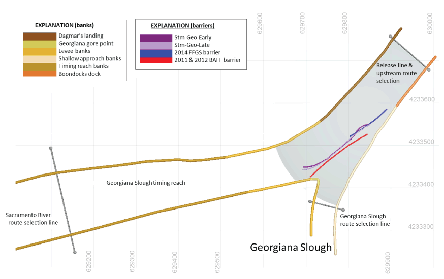
Georgiana Slough bank avoidance terms as applied to individual portions of the riverbanks. The three bold barrier designs are the resulting optimized barrier solutions for the three optimization simulations (table 1). The light grey shading represents the slow timing zone area and unshaded areas are fast timing zones. Grid spacing is in UTM Zone 10 Cartesian coordinate system.
The coordinates of the banks define the geographical constraints of the junction as observed at the high-water line and are hard coded into the IBM (figs. 9, 10, 15). For the BAFF it was discovered that within the observed fish tracks the actual location of the effective barrier surface moves because water velocities push against the bubbles. Initial efforts to align entrainment rates that did not account for the bubble barrier movement caused by water velocity did not converge well with the observed fish tracks of the prior studies. A BAFF deformation routine was added that predicted the effective barrier location at the surface. The deformation calculation interpolates the water velocities along the BAFF coordinates at each t to apply a deformation to the BAFF and relocate the BAFF coordinates accordingly. The deformation is based on a bubble rise rate of 0.25 meters per second (m/s) and a mean bubble diffuser depth of 2.4 meters (DWR, 2015).
After a simulated fish exhibits obstacle avoidance, two calculations are performed. First, an evasion speed (Se) is calculated from XSu during the last model t and its ASm. If Se is less than a minimum threshold Se is replaced with a minimum evasion speed (Sme). Sme is a safety value that assures that the simulated fish will always express enough energy to move away into better conditions. Sme is a calibration parameter and is set to 0.15 m/s. The second calculation is an avoidance vector normal to the closest bank or barrier being avoided. If the fish is within a response distance of both a bank and the barrier simultaneously, the two avoidance vectors are added together. The avoidance vector is then normalized to a unit vector of one to define the vector direction away from the object. The resulting unit vector is multiplied by Se or Sme, whichever is greater, to calculate an overall evasion vector (Ue). A water velocity vector is interpolated at the current simulated fish location and Ue is then added to the interpolated water vector to calculate Unet.
After avoiding an object, the simulated fish will continue along a new cross-stream direction during the subsequent model interval. Setting the cross-stream swimming direction away from the recently avoided obstacle simulates behavior documented during the 2012 BAFF study when fish often initiated sustained cross-stream movements away from the BAFF after encountering the barrier (DWR, 2015).
4.6. Advancing Model Time and Location
The IBM uses distance-based model intervals to determine the next simulated fish location and the elapsed time between each model t. The distance in each iteration is dependent on the behavioral mode, and a speed zone determined by the spatial coordinate of the simulated fish.
The spatial area of the wetted region bounded by the banks where simulated fish can be modeled is divided into two speed zone classifications, either slow zones, or fast zones. The zones are defined to decrease computational time within areas of the junction where high resolution is not required, while allowing better resolution in areas of greater importance. Slow zones focus on areas of interest such as around the barrier and directly around the junctions. Fast zones are areas such as the timing reaches on the downstream side of the junctions where object interaction is not as important (figs. 9, 10, 15).
Simulated fish in the out-migration behavioral mode move at a fixed distance every model iteration of 15 m while in the fast zone, and 5 m while in the slow zone. Simulated fish in obstacle avoidance behavioral mode move a fixed distance in each model iteration of 5 m in the fast zone and 0.25 m in the slow zone. Therefore, the IBM calculates the new location of the simulated fish by applying the appropriate fixed distance to the present simulated fish location in the direction of Unet. Elapsed time is calculated from the magnitude of Unet as a function of the selected fixed distance.
4.7. Finish Lines
Simulated fish movement is modeled until either the fish crosses one of the downstream finish lines, or until 18 hours of model time has passed. The 18-hour limit was chosen to allow enough time for tidal cycles to change and present stronger water velocities on ebb tides, while preventing conditions of impossible entrainment from holding up the IBM indefinitely. In rare cases, a simulated fish’s swimming parameters can cause the simulated fish to continuously swim upstream and overpower the magnitude of the water velocity. If the simulated fish has not crossed a finish line within 18 hours of model time, the model returns an error state and the simulated fish’s out-migration is terminated. This error occurred less than 0.15 percent of the time in an any of the optimization runs for this report due to simulated fish being assigned an aggressive upstream swimming behavior in low river flow conditions. When a simulated fish crosses one of the downstream finish lines their entrainment and model time are recorded in the Fish Object. The fish object is returned to STARS to allow the simulated fish to continue its out-migration, and the IBM ends the current session (fig. 2).
4.8. IBM Model Calibration
To calibrate the IBM for Georgiana Slough, the observed fish tracks that were collected under conditions without a barrier during the 2008 survival study (Holbrook and others, 2009) were compared to IBM simulated fish tracks. A simulated fish track was modeled using the first location of an observed fish track as the release location and the time of the observed track was used to select velocity maps. Swimming parameters were drawn at random which was repeated for each of the observed tracks 100 times. The observed and simulated fish tracks and their resulting routing probabilities where then compared (fig. 16). The discrepancies between the simulated and observed fish tracks were used to adjust the bank avoidance terms, Wv, and St, and the process was repeated until three cross-sectional distributions between simulated and observed tracks closely matched, and the entrainment probabilities were within roughly 3 percent. This calibration routine was repeated for Sutter Slough using tracks collected during the 2014 FFGS barrier study (DWR, 2016; fig. 17). Given that there is no fish track data for Steamboat Slough, the bank avoidance terms, Wv, and St from Sutter Slough were applied to Steamboat Slough.
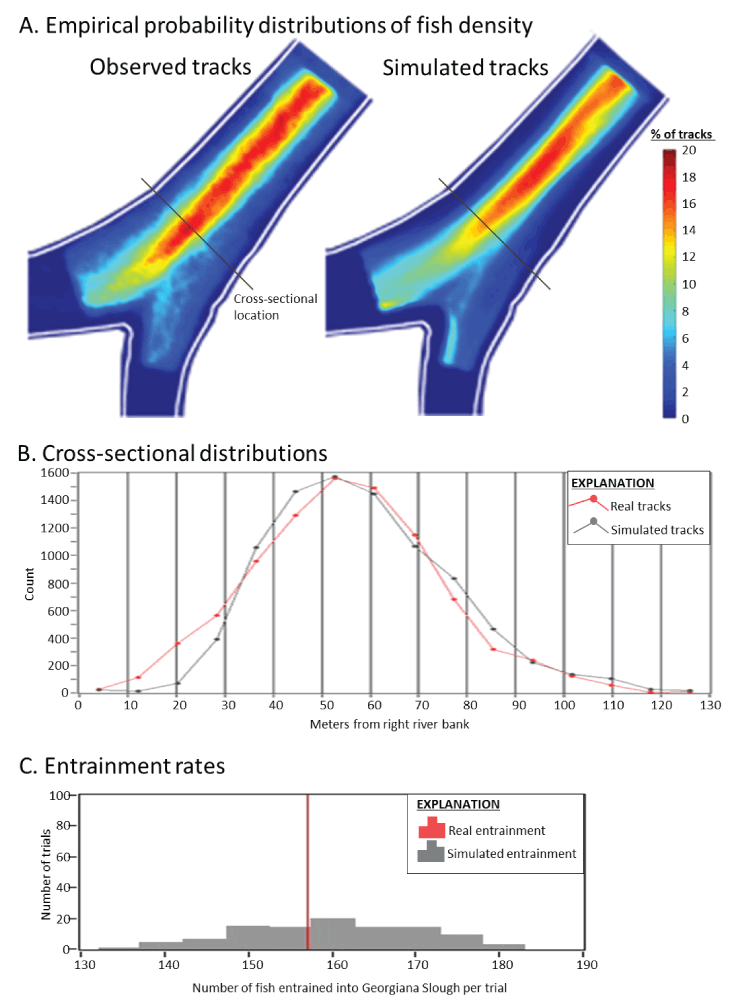
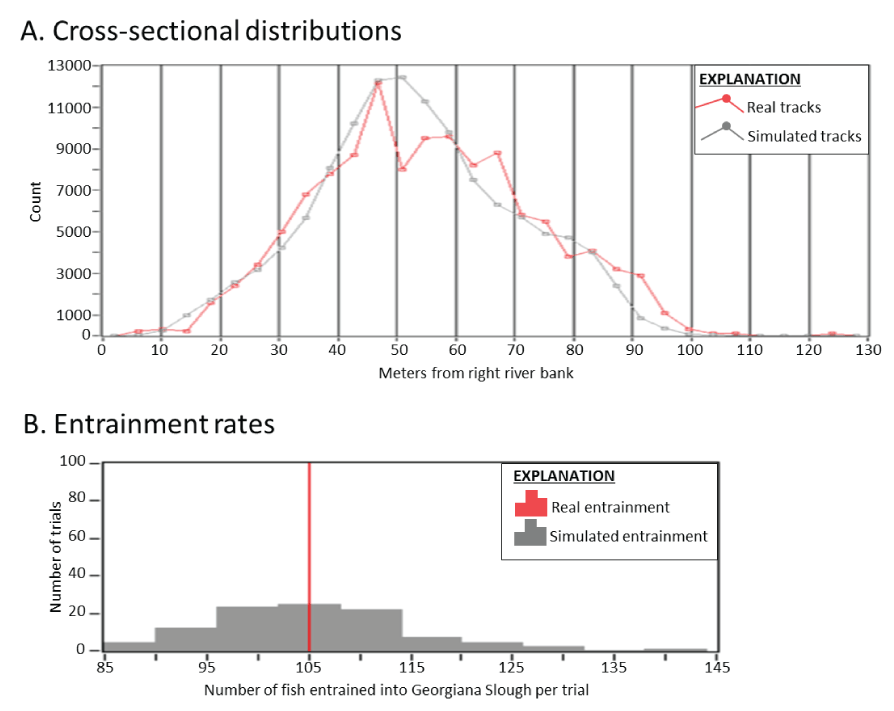
Density distributions and related routing probabilities of observed fish tracks collected during the 2008 telemetry study (Holbrook and others, 2009) to simulated fish tracks within Georgiana Slough, California. The percent density distribution of observed vs simulated tracks that passed through each 1-meter grid cell (A). The thin line shows the location of the cross-sectional comparison at the upper approach to the junction. The cross-sectional distribution of observed fish tracks to those of a series of simulated fish tracks released at the same location and water flow level to those of the observed tracks (B). The frequency of trials (N=100) that resulted in the number of entrained simulated fish per relative to the number of observed fish entrained in the 2008 telemetry study (C). Observed tracks were compared to the same number of simulated fish tracks, which is why there were 100 identical observed fish track trials.
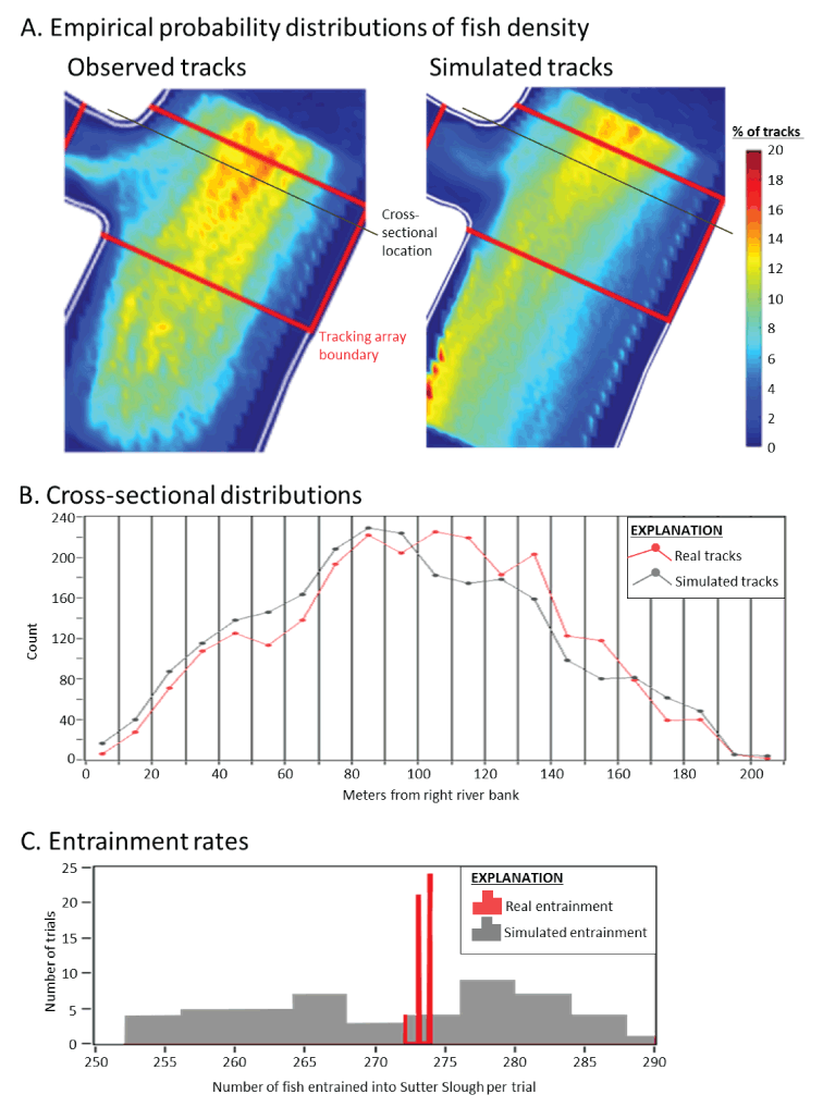
Density distributions and related routing probabilities of observed fish tracks collected during the 2014 telemetry study (DWR, 2016) to simulated fish tracks within Sutter Slough. The percent density distribution of observed vs simulated tracks that passed through each 1-meter grid cell (A). The thick red lines denote the region where observed tracks had higher precision within the deployed tracking array. The thin line shows the location of the cross-sectional comparison at the upper approach to the junction. The cross-sectional distribution of observed fish tracks to those of a series of simulated fish tracks released at the same location and water flow level to those of the observed tracks (B). The frequency of trials (N=100) that resulted in the number of entrained simulated fish per trail relative to the number of observed fish entrained in the 2014 telemetry study (C). In each trial the observed tracks were compared to the same number of simulated fish tracks. When a simulated fish track went upstream past the start line, both the observed and simulated fish tracks were censored from the analysis. This resulted in 5 trials where 2 fish were censored from the analysis and 21 trials where 1 fish was censored from analysis.
We then calibrated the IBM by adjusting the cross-stream distribution at the release line and the BAFF avoidance terms. First, we developed a routine that iteratively adjusted the release locations for flows that ranged from 10,000 to 100,000 ft3/s until routing probabilities without barriers were similar to those calculated in STARS. We then iteratively adjusted the mean and standard deviation for the BAFF barrier avoidance parameters to match the response distance from the BAFF by setting BAFF to the “on” condition which was then repeated until routing probabilities for simulated fish were similar to routing probabilities observed in the 2011 and 2012 BAFF studies when the BAFF was active (DWR, 2012, 2015; fig. 18).
Cross-sectional distributions and entrainment rates of simulated fish tracks versus observed tracks within Georgiana Slough when the 2011 and 2012 bioacoustic fish fences (BAFF) were operational. The cross-sectional distribution of observed fish tracks compared to those of a series of simulated fish tracks released at the same location and water flow levels (A). The frequency of trials (N=100) that resulted in the number of entrained simulated fish per trail relative to the number of observed fish entrained in the 2011 and 2012 BAFF barrier studies when the BAFF was operational (B). Observed tracks were compared to the same number of simulated fish tracks, which is why there were 100 identical observed fish track trials.
5.0. The Applied Computational Framework
Two computational strategies were implemented to improve the efficiency of the BOT. The first was to structure the STAIRS model into a modular framework of individual nodes we called a distributive model framework (DMF). The DMF allows the BOT to parallelize multiple STAIRS runs of the different candidates at the same time while using shared computational resources. The second was the use of a cloud-based infrastructure as a service (IaaS) platform to provide the computational resources. Roughly 87 million fish were independently modeled within each optimization run through STAIRS in roughly 36 hours using these two strategies.
5.1. Developing a Distributive Model Framework
The DMF was developed to efficiently run the STAIRS models in parallel. The DMF breaks individual decisions within STAIRS into independent processing steps called nodes. These independent nodes can be distributed among a cluster of servers. We developed a special language to facilitate communication among individual servers so that decisions can be shared allowing multiple simultaneous STAIRS model runs. Because each decision within STAIRS is determined by a single node, the individual sections of the model can be weighted based on their processing time and processing resource burden. Nodes with decisions that take more time and use more computer resources can be allocated among more servers to distribute the burden. Through this process STAIRS can be parallelized, and the computational requirements balanced over the available server clusters for the greatest speed and efficiency.
The portion of STAIRS performed by STARS are quicker processes than the portions performed in the junctions by the IBM. Without the DMF, STAIRS would have spent an unproportionally large amount of time working through the IBM routing while the rest of the model would have remained idle. With the DMF, the number of servers assigned to compute the IBM routing were greatly increased so that their burden could be distributed over a large pool of processing resources, thereby reducing idle time over the entire model and increasing overall efficiency.
5.2. Using IaaS for Computational Resources
The power of the DMF depends on the available computational resources that the framework can be distributed over. One of the fastest and most reliable ways to access computational resources is the use of cloud-based IaaS platforms. For this project an IaaS platform was used to create and control virtual computers that had our server optimization software installed on them. With this process, 250 virtual servers were created for each optimization run. IaaS services were duplicated across two clusters of resources which allowed two optimization efforts to run in parallel, thus using a total of 500 DMF servers. For each optimization run, 50 of the 250 servers were configured to run all the STARS based routing and survival estimates, and 200 were configured to run the IBM for Sutter, Steamboat, and Georgiana sloughs. Through this weighted approach the computational burden of the IBM was overcome, and optimization runs could finish in a fraction of the time that it took without the DMF.
The process of creating the DMF within the IaaS framework required an understanding of network protocols and security, along with a working knowledge of the IaaS architecture. We wrote a communication language for this project that uses Java Script Object Notation (Bassett, 2015) formatting as the underlying data structure that allowed individual servers to communicate with one another through Transmission Control Protocol/Internet Protocol (Falls and Stephens, 2012). The server dispatch layer is a compiled application that was specifically developed for this work. The overall scope of the DMF as it was applied within the IaaS platform is beyond the scope of this document. However, without this architecture it would be difficult to achieve the same number of optimization runs in a timely manner, given the same level of iterations and sample sizes of fish.
6.0. Running Optimizations
We ran three optimization efforts with the BOT. Each of these efforts explored different multi-junction barrier designs with different barrier operational periods. The first optimization effort explored possible FFGS barrier designs at Steamboat Slough and possible BAFF barrier designs at Georgiana Slough during a barrier operational period of November 1–March 15 (early operational period), henceforth referred to as Stm-Geo-Early. The second effort explored FFGS barrier designs at Steamboat Slough and BAFF barrier designs at Georgiana Slough with a barrier operational period from January 1 through April 30 (late operational period), henceforth referred to as Stm-Geo-Late. The third effort only explored FFGS barrier designs at Steamboat Slough. No barriers were implemented at Georgiana Slough. This effort used the late barrier operational period and is henceforth referred to as StmOnly-Late.
6.1. Model Accuracy and Precision
To assess model accuracy, survival estimates were compared between STARS and STAIRS models run with 100,000 fish per year in the absence of barriers. The STAIRS barrier-free survival of simulated fish was 51 percent, which was 1 percent less than the STARS barrier-free survival (52 percent) of simulated fish. The survival rates generated from this large-sample-size of the barrier-free STAIRS simulations represents a baseline survival scenario for contrast to all other modeled scenarios.
To examine how sample size may affect the precision of through-delta survival estimates we ran the STAIRS model over a range of sample sizes in the absence of any barriers. Ten iterations were run using six different sample sizes (table 2). The level of precision from this experiment showed a roughly plus or minus (±) 0.1 percent difference in percent survival with a simulated sample size of at least 15,000 fish. We then repeated this experiment with 60 iterations using 4 sample sizes (1,500, 7,500, 15,000, and 30,000). This experiment showed that a sample size of 15,000 fish converged to within ± 0.1 percent of the baseline survival (table 2). Although greater precision was reached with simulated sizes greater than 15,000, the benefit of increasing the sample size diminished. Given sample size, effort, and cost, we chose to run the BOT with 15,000 simulated fish for each candidate.
Table 2.
Through-delta percent survival statistics using salmon travel time and individual routing simulation (STAIRS) with varying simulated fish sample sizes.[All simulations were run in the absence of barriers.]
Evaluating Optimization Runs
Survival rates from the optimized barriers from each of the three BOT efforts were compared to the baseline survival estimates to assess the effectiveness of barrier designs derived in each optimization effort. To determine if effectiveness of the optimized barrier solutions were biased by a single barrier within the solution, we ran a series of scenarios with STAIRS where only one barrier at a time for each optimization solution was used. To disentangle the effect of barrier operational periods on barrier designs, barrier solutions from each scenario were modeled using the opposite barrier operational period (early or late) than originally run. In these non-optimized STAIRS simulations, a sample size of 100,000 simulated fish was used. To determine if the optimized barrier designs made an improvement over the 2011 and 2012 Georgiana BAFF studies (DWR, 2012, 2015), we ran scenarios that estimated STAIRS survival rates while using the 2011 and 2012 Georgiana BAFF coordinates within each of the operational periods.
7.0. Results
Through-delta survival of simulated fish was improved by 1.0–6.3 percent with one or more optimized barriers compared to the STAIRS barrier-free baseline survival rate of simulated fish (table 3). Simulated survival using the BAFF location in the 2011 and 2012 study was 3.1 percent greater during the late operational period and 5.2 percent greater during the early operational period than the STAIRS barrier free-baseline survival of simulated fish. Operational period had a strong effect on predicted survival. The early operational period (November 1–March 15) affected about 95 percent of out-migrating juvenile winter-run Chinook salmon and improved survival by roughly twice as much as the late operational period (January 1–April 30), affecting about 48 percent of out-migrants (fig. 19). Predicted simulated fish survival estimates for scenarios where Steamboat and Georgiana sloughs were both modeled with a barrier were similar to scenarios where only a barrier at Georgiana Slough was modeled. Survival estimates for simulated fish were lower when a barrier was only considered at Steamboat Slough. Optimized barrier designs at Steamboat Slough varied among runs and did not have a strong effect on through-delta survival of simulated fish (table 3).
Table 3.
Through-delta percent survival for the three optimization efforts (bold).[With additional salmon travel time and individual routing simulation (STAIRS) scenarios with varying barrier configurations or operational considerations. All results based on STAIRS runs with a simulated fish sample size of 100,000 fish. Barrier operational periods consisted of a late operational period from January 1 to April 30, and an early operational period from November 1 to March 15. Optimization efforts included consideration of barriers at Steamboat Slough (Stm), Georgiana Slough (Geo), or both. Efforts also considered combinations of barriers in early (Early) or late (Late) time periods.]
7.1. Optimization Stm-Geo-Early
In the Stm-Geo-Early optimization effort, the BOT ran for 56 iterations and tested approximately 5,800 unique barrier designs before candidates converged. The final optimized barrier design with the highest score in the Stm-Geo-Early scenario improved through-delta survival of simulated fish by 6.2 percent over the baseline model (table 3). This optimized solution included a 97 m long FFGS barrier at Steamboat Slough, extended from the middle right portion of the Sacramento River to the downstream end of the junction (fig. 9). The solution also included a 192 m long BAFF barrier at Georgiana Slough that was roughly parallel to the Sacramento River current (fig. 15; app. 1; table 1.1).
The improvement in survival over the baseline model was similar when we tested the barrier designed in the Stm-Geo-Early scenario for Georgiana Slough with and without the Steamboat Slough barrier over the early operational period (table 3). The Stm-Geo-Early Steamboat Slough barrier solution without the Georgiana barrier tested over the early operational period resulted in a small improvement in predicted through-delta survival of simulated fish over the baseline model. Tests in which the late operational period was applied with either barrier, but not both, resulted in only minimal improvements in predicted survival over the baseline model (table 3).
7.2. Optimization Stm-Geo-Late
In the Stm-Geo-Late optimization effort, the BOT ran for 56 iterations and tested approximately 5,800 unique barrier designs before candidates converged. The optimized barrier design under the Stm-Geo-Late scenario increased through-delta survival of simulated fish by 3.92 percent over the baseline (table 3). The Stm-Geo-Late Steamboat Slough optimized barrier design was 97 m long and starts about 64 m upstream of the Steamboat junction, about 15 m off the right bank of the Sacramento River. It then runs approximately perpendicular to the Sacramento River until it is almost in the center of the river. Then the barrier turns roughly 90° downstream and runs parallel to the river (fig. 9). The Georgiana Slough optimized barrier design under the Stm-Geo-Late scenario was 192 m long and was roughly parallel to the Sacramento River current (fig. 15; app. 1; table 1.2). The most notable difference between the Georgiana Slough barriers derived under the Stm-Geo-Early and Stm-Geo-Late scenarios is in the degree of curvature at the ends of the barriers.
The improvement in survival over the baseline model was similar when we tested the barrier designed in the Stm-Geo-Late scenario for Georgiana Slough with and without the Steamboat Slough barrier over the early operational period (table 3). When the Stm-Geo-Late Steamboat Slough barrier was modeled without a barrier at Georgiana Slough using the late operational period, the predicted improvement in survival over the baseline model was minor (table 3).
7.3. Optimization StmOnly-Late
In the StmOnly-Late optimization effort, the BOT ran for 57 iterations and tested approximately 5,900 unique barrier designs before candidates converged (app. 1; table 1.3). The StmOnly-Late Steamboat Slough barrier design resulted in a slight increase in survival over the baseline (table 3). StmOnly-Late resulted in a Steamboat barrier that starts roughly 20 m upstream of Steamboat Slough and about 50 m off the right bank of the Sacramento River. The 91-meter barrier turns directly onto the downstream point of the junction. The predicted survival was somewhat greater for the StmOnly-Late Steamboat barrier design when implemented over the earlier barrier operational period.
8.0. Discussion
8.1. Barrier Operational Timing Differences
The greatest difference in simulated fish through-delta survival of simulated fish among scenarios was attributable to differences in operational period. Over the 15 years of Knights Landing catch data used to simulate winter-run Chinook salmon run timing, the catches increased from mid-November to a peak in late December (fig. 19). Given that travel times of simulated fish between Verona and Steamboat Slough were two to four days (about 73 km travel distance), slightly fewer than 95 percent of simulated fish passing through a junction could be expected to encounter the barrier during the earlier operational period. The later operational period missed the peak of the December out-migration of juvenile winter-run Chinook salmon, resulting in roughly 48 percent of simulated fish arriving at a junction with a barrier and 52 percent arriving when no barrier was present.
8.2. Dissimilarity of Barrier Designs at Steamboat Slough
The route that provided the optimal survival of simulated fish at Steamboat Slough varied depending on the mean flow experienced within the operational period, and the routing probabilities downstream. When a barrier was modeled at Georgiana Slough, simulated fish were routed into Steamboat Slough given the early operational period. Whereas simulated fish were routed into the Sacramento River when the late operational period was implemented. When no barrier was included at Georgiana Slough and the late operational period was considered, the optimized barrier at Steamboat Slough routed fish into Steamboat Slough. The difference in routing at Steamboat Slough between Stm-Geo-Early and Stm-Geo-Late indicates occasional low flows and the low survival in the central Sacramento-San Joaquin River Delta. Overall, through-delta survival of simulated fish may still improve by sending fish down Steamboat Slough rather than exposing them to entrainment in Georgiana Slough. This is true even in the presence of a barrier at Georgiana Slough. However, when only higher flows were considered under the later operational period, it was advantageous to increase entrainment into Steamboat Slough with or without a barrier at Georgiana Slough. This is because entrainment of fish into Georgiana Slough is lower at higher flows that push fish past the junction than at lower flows when reversing tides push more fish back into Georgiana Slough. Therefore, we expect a fish guidance barrier that directs fish into Steamboat Slough to be most effective at low and reversing flows. Because barriers were optimized based on a range of flows rather than specific flows, we are unable to determine the specific flow where this shift in barrier shape at Steamboat Slough is advantageous.
Another factor contributing to the variation in barrier designs at Steamboat Slough is uncertainty in FFGS barrier avoidance terms. The FFGS avoidance terms applied were from fish tracks observed during the 2014 Georgiana Slough FFGS barrier study where very few tagged fish interacted with the FFGS (DWR, 2016; Romine and others, 2016), so we did not have a sufficient sample size to estimate the FFGS avoidance terms more accurately. Future work to clarify FFGS avoidance terms may help improve the ability of the BOT to optimize FFGS type barrier designs at Steamboat Slough.
8.3. Similarity of Barrier Designs at Georgiana Slough
The optimized barrier designs at Georgiana Slough were nearly identical between Stm-Geo-Early and Stm-Geo-Late scenarios and operational periods. When compared equally, the difference in predicted survival between these two barriers is less than the precision of the model. Differences within the flow range modeled had little effect on the shape of the barrier, indicating barrier designs performed similarly over the distribution of flows modeled. Given an increased frequency of low flows, such as those occurring over the past decade (2012–22), we expect greater entrainment in Georgiana Slough (fig. 12). Barriers optimized under frequent low flow conditions may take a different shape to reduce entrainment of fish heading upstream on incoming tides.
8.4. Optimizations Targeting Specific Flow Levels
The simulation period that we used in the BOT resulted in barrier designs that increased survival over full range of flows in the period of record, but not necessarily at any specific low flows. The distribution of Sacramento River flows at Freeport were similar during the simulation period (1997–2011) as they were for the full period of record (1948–2022), and more frequently higher than they were in the last decade (2012–22; figs. 12, 20). Flows less than 18,000 ft3/s, when tidal influence can reverse flows at Georgiana Slough, were about 20 percent more frequent in the last decade than over the entire period of record (figs. 12, 20). Optimizations run at lower flows, especially those less than 18,000 ft3/s, may result in different optimized barrier shapes. For example, a low-flow-optimized barrier at Georgiana Slough may result in a barrier that diverts fish from approaching Georgina Slough from both upstream and downstream. As mentioned previously, barriers optimized under low flow conditions would also be more likely to divert fish into Steamboat Slough. Alternatively, under low and reversing flows, the BOT may have trouble converging on a barrier at Georgiana Slough given the cost constraints applied in these efforts. A barrier design would likely need to be much longer than we allowed to prevent fish from entering the slough from both directions.
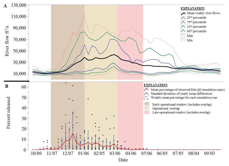
Winter-run Chinook salmon (Oncorhynchus tshawytscha) timing at Knights Landing, California and relating river flows. Bars highlight the date ranges of the applied barrier operational periods used within the optimization efforts. The mean weekly river flows at Freeport, California within the 15-year simulation period, the 25th and 75th percentiles, the 10th and 90th percentiles, and the minimum and maximum river flows observed (A). The weekly percentage of the annual catch at Knights Landing for all 15 years of the simulation period from 1997 to 2011, the standard deviations within the individual years of the simulation period and the weekly percentage for each year (B).
9.0. Summary and Conclusion
We developed the barrier optimization tool (BOT) to design behavioral fish barriers at up to three junctions within the Sacramento-San Joaquin Delta for improving through-delta survival of juvenile winter-run Chinook salmon (Oncorhynchus tshawytscha). The BOT uses a machine learning approach to test candidates by simulating fish through-delta passage using the salmon routing time and travel simulation (STARS) model (Perry and others, 2019) modified by replacing probabilistic route determination at junctions with an individual based model (IBM). The IBM is a particle tracking model modified to include fish behavior and the combined modified model is called salmon travel time and individual routing (STAIRS). We used the BOT to optimize barrier designs at Georgiana and Steamboat sloughs given three efforts that differed in combination of barriers tested and operational period.
The BOT generated optimized barrier designs that improved though-delta survival by as much as 6.3 percent over survival under the STAIRS baseline barrier-free scenario. These optimized barrier designs also improved survival over the 2011 and 2012 Georgiana Slough barrier configuration, which was designed based on professional judgement (DWR, 2012, 2015). This indicates that the BOT is an effective tool for designing barrier configurations that potentially can help fishery managers increase survival of out-migrating juvenile salmonids through the Sacramento-San Joaquin Delta.
Operational period was the most influential factor for improving through-delta survival in our simulations. Fifty-seven percent more simulated fish entered a junction with a barrier present given the early operational period from November 1 through March 15 than the late operational period from January 1 to April 30. This resulted in a 2.3–2.6 percent greater survival with implementation of an early operational period than implementation of a late operational period that considered a Georgiana Slough barrier. The difference in survival when the late and early operational periods were compared with only a Steamboat Slough barrier was less than the difference between the STARS and STAIRS model comparisons (1 percent; see “6.1 Model Accuracy and Precision”).
Given that the distribution of flows used in optimizations (1997–2011) were similar to the historical record (1948–2022), a barrier at Georgiana Slough was more effective than a barrier at Steamboat Slough, when considered independently. The shape of the optimized Steamboat Slough barriers routed fish into Steamboat Slough when more frequent low flow conditions were modeled than when more frequent high flows were modeled. The Steamboat Slough barriers also routed fish into Steamboat Slough when a Georgiana Slough barrier was absent, but into the Sacramento River and past the Georgiana Slough junction, when a Georgiana Slough barrier was present. In contrast, the barriers designed at Georgiana Slough were nearly identical among scenarios. We caution that barriers designed by the BOT for Georgiana Slough may be less effective than predicted given the more frequent low flows of the past decade (2012–22).
The most effective barrier design, that was chosen for implementation by the California Department of Water Resources (DWR), was based on a BAFF designed under a scenario that included a barrier at both Steamboat Slough and Georgiana Slough junctions over the late operational period (fig.16, app. 1, table 3). The design was made more successful by including only a Georgiana Slough barrier over the earlier operational period.
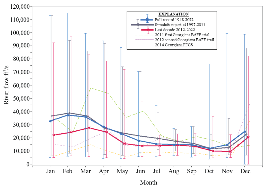
Mean monthly river flows for barrier-optimization-tool relevant time periods. For periods of time larger than a single year, error bars show the range of the minimum and maximum experienced flows within that period. Mean monthly flows are given for the periods of time in which the 2011, 2012, and 2014 barrier trials were conducted.
References Cited
California Data Exchange Center, 2022, Historical data query, California Department of Water Resources, accessed September 25, 2023, at https://cdec.water.ca.gov.
Columbia Basin Research, 2022, SacPAS: Central Valley prediction and assessment of salmon through ecological data and modeling for in-season management: University of Washington School of Aquatic and Fishery Sciences, Columbia Basin Research, accessed September 25, 2023, at https://www.cbr.washington.edu/sacramento/.
Hance, D.J., Perry, R.W., Burau, J.R., Blake, A., Stumpner, P., Wang, X., and Pope, A., 2020, Combining models of critical streakline and the cross-sectional distribution of juvenile salmonids to predict fish routing at river junctions: San Francisco Estuary and Watershed Science, vol. 18, no.1, p.1–17, accessed December 6, 2023, at https://doi.org/10.15447/sfews.2020v18iss1art3.
Holbrook, C.M., Perry, R.W., and Adams, N.S., 2009, Distribution and joint fish-tag survival of juvenile Chinook salmon migrating through the Sacramento-San Joaquin River Delta, California, 2008: U.S. Geological Survey Open-File Report 2009–1204, 30 p, accessed July 29, 2021, at https://pubs.usgs.gov/of/2009/1204/.
Perry, R.W., Skalski, J.R., Brandes, P.L., Sandstrom, P.T., Klimley, A.P., Ammann, A., and MacFarlane, B., 2010, Estimating survival and migration route probabilities of juvenile salmon in the Sacramento-San Joaquin River Delta: North American Journal of Fisheries Management, v. 30, no. 1, p. 142–156, accessed December 6, 2023, at https://doi.org/10.1577/M08-200.1.
Perry, R.W., Romine, J.G., Adams, N.S., Blake, A.R., Burau, J.R., Johnston, S.V., and Liedtke, T.L., 2012, Using a non-physical behavioral barrier to alter migration routing of juvenile Chinook salmon in the Sacramento-San Joaquin River Delta: River Research and Applications, v. 30, no. 2, p. 193–203, accessed December 6, 2023, at https://doi.org/10.1002/rra.2628.
Perry, R.W., Brandes, O.L., Burau, J.R., Klimley, A.P., MacFarlane, B., Michel, C., and Skalski, J.R., 2013, Sensitivity of survival to migration routes used by juvenile Chinook salmon to negotiate the Sacramento San Joaquin River Delta: Environmental Biology of Fishes, v. 96, nos. 2–3, p. 381–392, accessed December 6, 2023, at https://doi.org/10.1007/s10641-012-9984-6.
Perry, R.W., Brandes, P.L., Burau, J.R., Sandstrom, P.T., and Skalski, J.R., 2015, Effects of tides, river flow, and gate operations of entrainment of juvenile salmon into the interior Sacramento-San Joaquin River Delta: Transactions of the American Fisheries Society, v. 144, no. 3, p. 445–455, accessed December 6, 2023, at https://doi.org/10.1080/00028487.2014.1001038.
Perry, R.W., Pope, A.C., Romine, J.G., Brandes, P.L., Burau, J.R., Blake, A.R., Ammann, A.J., and Michel, C.J., 2018, Flow-mediated effects on travel time, routing, and survival of juvenile Chinook salmon in a spatially complex, tidally forced river delta: Canadian Journal of Fisheries and Aquatic Sciences, v. 75, no. 11, p. 1886–1901, accessed December 6, 2023, at https://doi.org/10.1139/cjfas-2017-0310.
Perry, R.W., Pope, A.C., and Sridharan, V.K., 2019, Using the STARS model to evaluate the effects of the proposed action for the reinitiation of consultation on the coordinated long-term operation of the Central Valley and State Water Project: U.S. Geological Survey Open-File Report 2019–1125, 31 p. plus appendixes, accessed June 22, 2021, at https://pubs.usgs.gov/of/2019/1125/ofr20191125.pdf.
Romine, J.G., Perry, R.W., Pope, A.C., Stumpner, P., Liedtke, T.L., Kumagai, K.K., and Reeves, R.L., 2016, Evaluation of a floating fish guidance structure at hydrodynamically complex river junction in the Sacramento-San Joaquin River Delta, California, USA: Marine and Freshwater Research, v. 68, no. 5, p. 878–888, accessed December 6, 2023, at https://doi.org/10.1071/MF15285.
U.S. Geological Survey, 2023, USGS water data for the Nation: U.S. Geological Survey National Water Information system database, accessed September 25, 2023 at https://nwis.waterdata.usgs.gov/nwis/dv.
Appendix 1. Geographical Locations of Optimized Barriers for Optimization Simulation
Table 1.1.
Cartesian coordinates in Universal Transverse Mercator (UTM) zone 10, and in latitude and longitude (in decimal degrees) of the best barrier solutions are identified by optimization simulation in which barriers at both Steamboat and Georgiana sloughs in the early period were considered (Stm-Geo-Early).[These points define beginning and ends of each barrier panel section sequentially.]
Table 1.2.
Cartesian coordinates in Universal Transverse Mercator (UTM) zone 10, and in latitude and longitude (in decimal degrees) of the best barrier solutions are identified by optimization simulation in which barriers at both Steamboat and Georgiana sloughs in the late period were considered (Stm-Geo-Late).[These points define beginning and ends of each barrier panel section sequentially.]
Table 1.3.
Cartesian coordinates in Universal Transverse Mercator (UTM) zone 10, and in latitude and longitude (in decimal degrees) of the best barrier solutions identified by optimization simulation in which barriers at only Steamboat Slough in the late period were considered (Stm-Geo-Early).[These points define beginning and ends of each barrier panel section sequentially.]
Conversion Factors
Abbreviations
ASm
along stream mean: The effort that a simulated fish will apply in the along stream water velocity vector at each iteration of a simulated fish’s movement within the flow field. It is part of a simulated fish's swimming parameters assigned at each individual based model call and can be negative or positive, expressing positive or negative rheotaxis respectively.
BAFF
bioacoustic fish fence: A non-physical fish guidance structure that utilizes a continuous wall of air bubbles released above the bed floor of the riverbed. In conjunction, the bubbles are inundated by light and sound created by underwater lighting and speakers positioned above the bed floor.
BOT
barrier optimization tool
Di
distance of response: The selected response distance of a bank or barrier drawn from a normal distribution with a mean and standard deviation specific to that bank or barrier type. Di is drawn at each model interval for every bank and barrier to add stochasticity within the avoidance response behaviors.
Dfm
A selected fractional multiplier drawn from a normal distribution of a mean of 0.207 and a standard deviation of 0.025 that is applied to the maximum cross-stream velocity within each cross-stream transect to determine the water velocity trigger (Wv) at each model interval.
FFGS
floating fish guidance structure: A physical fish guidance structure that consists of a series of floating panels linked together to create a physical barrier extending from the surface of the water to some depth below.
IBM
individual based model: A particle tracking model modified to include fish behavior.
Qa
Upstream 15-minute average river flow above a junction.
Qb
Downstream 15-minute average river flow in one of the downstream branches below a junction.
Se
speed of evasion: An avoidance behavior parameter used to apply a speed component to an avoidance vector. It is calculated from the simulated fish’s along stream mean (ASm) and cross-stream effort (XSu).
Sme
minimum speed of evasion: If the speed of evasion (Se) is lower than a specific value Se is replaced with Sme. This value was set to a constant of 0.15 meters per second. This ensures that simulated fish always express enough energy to escape areas of very low water velocity.
St
speed turbulence tuning: A type of turbulence tuning that is applied to the water velocity flow field through a log linear random perturbation based on the proximity to a bank object. It is added at each iteration of fish movement to the flow field if closer than 6 meters near banks to scale velocities toward zero as fish approach the bank. This is used to overcome the coarse accuracy of the flow fields in relation to the lack of water velocity measurements near shorelines. It makes sure simulated fish are not advected through bank objects because of unrealistic velocities near shore.
STARS
salmon travel time and routing simulation
STAIRS
salmon travel time and individual routing simulation
Sv
The water velocity scaling factor applied to the flow field velocity maps measured in 2014 to scale them to the historic Sacramento River flows as measured at the current model simulation time when greater than the observed flows in 2014.
Ue
evasion vector: The calculated vector a simulated fish will move away from objects while in obstacle avoidance mode. Ue is calculated by speed of evasion (Se) or minimum speed of evasion (Sme) for the speed component of the vector and combined with a vector directional component that is calculated to avoid an object. This is prior to any water velocity components.
Unet
movement vector: The total displacement vector calculated at every model interval within the IBM that is applied to the simulated fish for its overall movement.
Wv
water velocity trigger: A velocity value calculated from the mean cross-stream experienced velocities within a single cross-sectional excursion of a simulated fish multiplied by Dfm. If the current simulated fish’s cross-stream velocity falls below the Wv it triggers a change in the simulated fish’s cross-section direction.
XSm
cross-stream mean: The mean cross-stream effort calculated from each observed fish track. It is part of a simulated fish's swimming parameters assigned at each individual based model call.
XSstd
cross-stream standard deviation: The standard deviation of the cross-stream swimming velocity of observed fish with a mean of the cross-stream mean (XSm). It is part of a simulated fish's swimming parameters assigned at each individual based model call.
XSu
cross-stream effort: The selected value that a simulated fish will apply in the cross-sectional movement perpendicular to the water velocity at the current simulated fish location. This value is drawn out of a normal distribution from the cross-stream mean (XSm) and the cross-stream standard deviation (XSstd).
For information about the research in this report, contact:
Director, Western Fisheries Research Center
U.S. Geological Survey
6505 NE 65th Street
Seattle, Washington 98115-5016
https://www.usgs.gov/centers/wfrc
Manuscript approved on November 27, 2023
Publishing support provided by the U.S. Geological Survey
Science Publishing Network, Tacoma Publishing Service Center
Disclaimers
Any use of trade, firm, or product names is for descriptive purposes only and does not imply endorsement by the U.S. Government.
Although this information product, for the most part, is in the public domain, it also may contain copyrighted materials as noted in the text. Permission to reproduce copyrighted items must be secured from the copyright owner.
Suggested Citation
Swyers, N.M., Blake, A., Stumpner, P., Burau, J.R., Burdick, S.M., and Anwar, M.S., 2024, A machine learning tool for design of behavioral fish barriers in the Sacramento-San Joaquin River Delta: U.S. Geological Survey Open-File Report 2023–1095, 38 p., https://doi.org/10.3133/ofr20231095.
ISSN: 2331-1258 (online)
Study Area
| Publication type | Report |
|---|---|
| Publication Subtype | USGS Numbered Series |
| Title | A machine learning tool for design of behavioral fish barriers in the Sacramento-San Joaquin River Delta |
| Series title | Open-File Report |
| Series number | 2023-1095 |
| DOI | 10.3133/ofr20231095 |
| Publication Date | January 16, 2024 |
| Year Published | 2024 |
| Language | English |
| Publisher | U.S. Geological Survey |
| Publisher location | Reston, VA |
| Contributing office(s) | California Water Science Center, Western Fisheries Research Center |
| Description | ix, 38 p. |
| Country | United States |
| State | California |
| Other Geospatial | Sacramento-San Joaquin River Delta |
| Online Only (Y/N) | Y |