

Satellite Interferometry Landslide Detection and Preliminary Tsunamigenic Plausibility Assessment in Prince William Sound, Southcentral Alaska
Links
- Document: Report (11.3 MB pdf) , HTML , XML
- NGMDB Index Page: National Geologic Map Database Index Page (html)
- Download citation as: RIS | Dublin Core
Abstract
Regional mapping of actively deforming landslides, including measurements of landslide velocity, is integral for hazard assessments in paraglacial environments. These inventories are also critical for describing the potential impacts that the warming effects of climate change have on slope instability in mountainous and cryospheric terrain. The objective of this study is to identify slow-moving landslides in the Prince William Sound region, southcentral Alaska, United States, which has had rapid deglaciation since the mid-1800s, and assess their tsunamigenic plausibility. We use an automated time series persistent scatterer interferometric synthetic aperture radar processing method with 7 years of Sentinel-1 data (2016–22) to identify 43 slow-moving slopes with average velocities ranging from approximately 0.2 to 21 millimeters per year. Landslide presence is confirmed using aerial imagery and previous landslide inventory records. We assess the tsunamigenic plausibility of the landslides using empirically derived estimates of landslide mobility based on modeled landslide volumes. Of the identified landslides, our preliminary analysis suggests that 11 have tsunamigenic potential if they were to fail rapidly and catastrophically. Although our estimate of tsunamigenic plausibility is preliminary and can be refined with additional observations and analyses, it can be used to prioritize ongoing and future hazard assessment, surveillance, and research efforts.
Introduction
As glaciers thin and retreat in response to climate change, potentially unstable slopes are increasing in subarctic regions (for example, refer to Haeberli and others, 1997; Holm and others, 2004; Allen and others, 2009; Coe and others, 2018; Higman and others, 2018; Bessette-Kirton and Coe, 2020; Coe 2020; Dai and others, 2020; Klimeš and others, 2021; Fan and others, 2022; Svennevig and others, 2022; Kim and others, 2022; Penna and others, 2023). Subaerial landslides adjacent to open water that fail catastrophically (catastrophic failure defined herein as a landslide that suddenly moves at a speed that is faster than most humans can run, in other words, greater than about 4 meters per second or 10 miles per hour) have the potential to generate tsunamis that can be highly destructive not only in the immediate vicinity of the landslides (for example, Blikra and others, 2006; Higman and others, 2018), but also across broad regions (for example, Harbitz and others, 2014). These landslide-generated tsunamis can affect life, marine traffic, and the built and natural environment. Measuring the displacement rates of unstable slopes allow for a better understanding of how slope stability conditions change throughout space and time due to glacial processes, climate variability, and other transient movement-forcing phenomena (Ballantyne, 2002; McColl, 2012). Landslide velocity and changes in velocity also serve as critical inputs in landslide hazard assessments (for example, Hermanns and others, 2013). On a regional scale, satellite remote sensing that identifies deformation (for example, methods using synthetic aperture radar [SAR] data; Lu and Kim 2021; Kim and others, 2022) or detects change associated with movement (for example, methods using multispectral data; Nichol and Wong, 2005; Ramos-Bernal and others, 2018) can provide the spatial and temporal resolution required to better understand landslide initiation, kinematics, and triggering conditions.
One area with rapid glacier retreat is the Prince William Sound region in southcentral Alaska (United States) (fig. 1). Prince William Sound is surrounded by the glaciated Chugach Mountains, which rise from sea level to nearly 4,000 meters (m) in a horizontal distance less than 20 kilometers (km). This region has 25,000 square kilometers (km2) of waterways and over 150 tidewater and valley glaciers. The Chugach Mountains primarily consist of the Cretaceous Chugach flysch accretionary complex (for example, Wilson and others, 2015 and references therein). In general, and in Alaska, flysch (alternating sandstone-siltstone beds) is highly susceptible to rock-slope failures (for example, Duman and others, 2005; Margielewski, 2006; Bessette-Kirton and Coe, 2020; Kim and others, 2022). The identification of a large moving landslide with tsunamigenic potential in Barry Arm (Dai and others, 2020; Barnhart and others, 2021; Coe and others, 2021; Schaefer and others, 2020; Schaefer and others, 2022; Schaefer and others, 2023) motivates the construction of a more comprehensive inventory of other potentially tsunamigenic landslides in this region.
In this report, we used automated persistent scatterer interferometric synthetic aperture radar (PSInSAR) processing of Sentinel-1 synthetic aperture radar (SAR) data to identify mountainous bedrock slopes in the Prince William Sound region of Alaska (refer to study area outlined in figure 1, approximately 40,500 km2) that moved very slowly to extremely slowly (less than or equal to 16 mm/yr to1.6 m/yr as classified in the International Geotechnical Societies’ United Nations Educational, Scientific and Cultural Organization [UNESCO] Working Party on World Landslide Inventory [WP/WLI; WP/WLI, 1995]) between 2016 and 2022. While slow-moving landslides do not necessarily represent a hazard, rapid acceleration of slowly deforming landslides has been observed prior to catastrophic failure in other locations (Hermanns and others, 2013). We confirmed landslide presence and estimated landslide area using a combination of ascending and descending SAR tracks, optical imagery and digital terrain data, and previous landslide inventories. A preliminary assessment of tsunamigenic potential was then performed using empirically derived estimates of landslide mobility combined with estimated landslide volumes. The data in this report are intended to provide a preliminary means of assessing the potential hazard of the landslides identified using PSInSAR and to assist in the prioritization of future research, surveillance, and hazard assessment efforts.
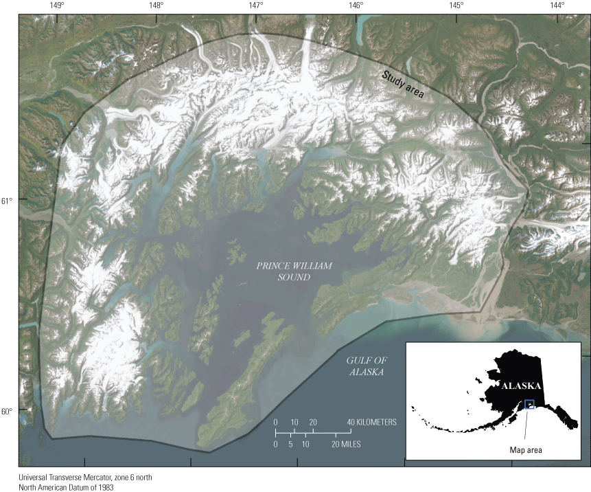
Map showing the study area of the Prince William Sound, roughly 40,500 square kilometers. Inset indicates location of Prince William Sound in southcentral Alaska.
Methodology
The following section describes methods used to (1) identify moving slopes, (2) confirm landslide presence and delineate landslide boundaries, (3) calculate landslide volumes, and (4) assess whether catastrophic failure of the landslide could produce a tsunami.
Persistent Scatterer Interferometric Synthetic Aperture Radar
We used PSInSAR to identify ground deformation in the Prince William Sound region using Sentinel-1 satellite images acquired during snow-free months (typically June–October) from 2016 through 2022. Persistent scatterer interferometric synthetic aperture radar quantifies phase differences at locations that exhibit consistent reflection and high coherence (in other words, there is little loss or change in radar reflectance) through a long period of time. These stable natural and artificial reflectors are known as persistent scatterers (PSs; for example, Ferretti and others, 2001; Hooper and others, 2004). Unlike traditional differential interferometric synthetic aperture radar (InSAR), which measures differences in the phase of returning waves between two SAR images, the use of PSs throughout a long temporal series of InSAR images in the PSInSAR technique allows for the extraction of useful phase information on a sparse grid of targets. This method can correct baseline-induced artifacts, digital elevation model (DEM) errors, and atmospheric disturbances through spatiotemporal regression and filtering. This permits the creation of time series of subtle (on the order of 10s of millimeters) ground deformation (Ferretti and others, 2001; Hooper and others, 2004; Hooper, 2008; Lu and Kim, 2021) and is effective in identifying landslides in paraglacial regions (Kim and others, 2022).
Differential interferograms throughout the study area were generated and stacked using methods described in Kim and others (2022). Stacked interferograms were then processed using the Stanford method for persistent scatterers PSInSAR technique (Hooper and others, 2004; Hooper, 2008). Persistent scatterers candidates were initially chosen based on pixels with lower values of variations in amplitude using the amplitude dispersion index (Ferretti and others, 2001), which corresponds to scatterers with a higher signal-to-noise ratio and thus better quality of phase. The PS probability was then estimated by iterative phase analysis (eq. 1) based upon the phase decorrelation noise, , which describes the variance in the residuals between observed and estimated phase at the PS candidate pixel (Hooper and others, 2004):
whereN
is the number of interferograms;
is the wrapped phase of pixel in the ith interferogram;
is the evaluated spatially uncorrelated look angle error factor; and
is the estimation of the spatially correlated factor.
The iterative process continues, and the solution converges, until is no longer decreasing (Hooper, 2008; Qu and others, 2022). The resulting phase values of the PS candidates then go through processing steps that consist of DEM error correction, phase unwrapping, atmospheric filtering, and geocoding while maintaining the original resolution of SAR acquisitions (for Sentinel-1, 5 m by 20 m in range and azimuth, respectively) based on the geometry between the satellite orbit and the elevation of each pixel. This results in a time series of phase differences (in other words, ground deformation) for each PS.
Ascending satellite scenes for snow-free months for the years 2016–21 and descending satellite scenes for snow-free months for the years 2016–22 for Sentinel-1 tracks P014 (ascending, 162 scenes between June 9, 2016, and October 24, 2022), P065 (descending, 102 scenes between June 1, 2016, and October 27, 2021), P094 (ascending, 128 scenes between June 3, 2016, and October 29, 2021), and P160 (descending, 114 scenes between August 8, 2018, and October 22, 2022) were used in PSInSAR processing and are available from Alaska Satellite Facility’s vertex platform (https://search.asf.alaska.edu/) and the European Space Agency’s Copernicus Open Access Hub (https://scihub.copernicus.eu/). All movement described is one dimensional in the line of sight (LOS) of the satellite, where positive values indicate that distances between the satellite and the ground surface have become shorter, and negative values indicate that distances have become longer. It is assumed that the rate of deformation during snow-covered (and therefore decorrelated) periods follows that during the previous epoch, and each epoch and its following snow-free season is bridged by InSAR observations to minimize the effect of the winter period of no data.
Landslide Delineation and Confirmation
Landslide presence and precise geospatial extent inherently have some degree of uncertainty because of the partially qualitative nature of landslide identification (Guzzetti and others, 1999). To minimize this uncertainty, we visually assessed the PSInSAR results to identify contiguous areas greater than 50,000 square meters (m2) that exhibited deformation during the analysis period. This area threshold corresponds to the typical landslide minimum size found in an optical landslide inventory of northwest Prince William Sound (Higman and others, 2023), and allows us to reduce the inclusion of false positives because of other deformation phenomena in the area of interest (for example, localized deformation because of glacial processes). The identification of deforming slopes was confirmed using two or more SAR tracks. Once these preliminary areas were defined, we use optical satellite imagery and digital elevation data to identify features indicative of slope instability processes, including scarps, tension cracks, and signs of surface activity (for example, rockfall). Optical satellite imagery with 0.5-m resolution was sourced from Maxar’s WorldView (Maxar, 2023). Digital elevation data sources were obtained from the Alaska Division of Geological & Geophysical Surveys’ Elevation Portal (Alaska Division of Geological & Geophysical Surveys, 2023), including the statewide 5-m interferometric synthetic aperture radar DEM and local airborne light detection and ranging (lidar) datasets.
For each identified instability, a speculative perimeter polygon was manually delineated to calculate landslide area. The perimeter was drawn to circumscribe the PSInSAR points that showed deformation; exceptions to this approach occurred when clear lineations associated with slope deformation (for example, antiscarps, normal scarps, tension cracks, strike-slip faults) were visible in aerial imagery, or if the landslide has been previously delineated using high resolution imagery (for example, Coe and others, 2021). Where possible, the upslope extent of the landslide was defined based on the highest altitude normal scarps, the lateral extents were defined along shear zones, and the lower extent was assumed to be within some area of the slope. Owing to a lack of high-resolution bathymetric data, only subaerial portions of the landslide were considered. Resulting landslide polygons represent only a plausible extent of the landslide boundary, and therefore, landslide delineation and calculated landslide area are estimates that should be revised if additional data become available.
Landslide Volume
Because of uncertainty in the depth and geometry of the landslide failure surfaces, a range of landslide volumes were approximated using logarithmic spirals and volume-area (V-A) relations. Logarithmic spirals were calculated using a python package digger (Barnhart and others, 2023), using methods described in Barnhart and others (2021). Work at Barry Arm (Dai and others, 2020; Schaefer and others, 2023) suggests that the basal failure surface is likely curved, which suggests that a logarithmic spiral geometry is valid to use for landslides in flysch. In polar coordinates (r, θ), a logarithmic spiral is defined as follows:
whereThe elevations and locations of the landslide headscarp and toe imply an average ground surface slope of Φ. Equation 2 and the location of the headscarp and toe along the logarithmic spiral line can be rearranged to generate the following relation (eq. 3) among Φ, the headscarp angle α, and the toescarp angle β:
in which C is equivalent to 1. However, similar logarithmic spirals can be constructed with lower values of C. To determine the volume of each landslide, the location of the headscarp, toe, and headscarp angle was specified for a series of downslope-oriented transects spaced 50 m apart. The smallest volumes were constructed using a headscarp angle of 45 degrees and C equals 1, and the largest landslide volumes were constructed with a headscarp angle of 60 degrees and C equals 0.5, using methods in Barnhart and others (2021).Additionally, we calculated an estimated volume (V, in cubic meters [m3]) of the landslide based on surface area (A, in m2) using the V-A scaling power law for bedrock landslides defined in equation 4 as follows:
whereα
0.186 and
γ
1.35 (Larsen and others, 2010).
All volume calculations consider only the scenario in which the entire delineated subaerial extent fails catastrophically; in other words, no partial failure scenarios were considered. Thus, none of the reported volume estimates should be considered the smallest possible failure for a given location. Additionally, it is plausible that landslide failure could mobilize adjacent ground not included in the defined extent, which would increase the total volume of failed material. Landslide volume is an important input into the subsequent tsunamigenic plausibility assessment, but volume determination based on aerial extent and V-A scaling and modeling is imprecise and replete with uncertainty. Using a range of potential landslide volumes reflects this uncertainty.
Tsunamigenic Plausibility Assessment
Because of the remoteness of the study area and lack of substantive infrastructure contained within, the primary concern in this initial assessment of landslide hazard is the potential for catastrophic failure of a given landslide into waterbodies, and the corresponding tsunami generation. Given the preliminary nature of this report, we relied upon simple, empirically derived estimates of landslide mobility to characterize the tsunamigenic potential of identified instabilities using the method described in Scheidegger (1973). In other locations, this method has been accepted as a conservative approach for estimating the potential runout and tsunami generation of identified landslides (Hermanns and others, 2012). Two steps are required for this method. First, the potential reach of the landslide was determined using the scaling relations (eq. 5) derived by Scheidegger (1973), where a mobility estimate (F) can be calculated as follows:
whereV
is the landslide volume estimated by the methods described in the “Landslide Volume” section,
a
−0.15666, and
b
0.62419.
The mobility index F is inversely related to landslide travel distance, so a low value of F indicates a long travel distance, and a high value of F indicates a short travel distance. Mobility index F was calculated for all three volume methods described in the “Landslide Volume” section.
Second, we compared F to the mobility required for the landslide to reach the nearest shoreline. Accurate calculation of Fshore requires two processing steps: (1) calculation of the height of the “top” of the landslide, and direction and length of the fall line from the calculated top to the bottom of the landslide (Hslide, Lslide; fig. 2), and (2) calculation of the height and length of the runout path from the landslide to the nearest water body (Hpath, Lpath; fig. 2). To determine the maximum height used in the calculation, we first identified the slope aspect of the area-weighted center (or centroid) of the landslide polygon to define bearing (compass direction) of the fall line during landslide failure. The fall line (A–A' in figure 2), was then defined as a straight line from the top of the landslide, through the center of mass, and terminating at the bottom of the landslide below the center of mass on that same bearing. The variables Hslide and Lslide were then defined as the elevation difference and planimetric distance from A–A', respectively (fig. 2). Elevation and slope aspect were calculated using the 5-m interferometric synthetic aperture radar-derived DEM available for Alaska (Alaska Division of Geological & Geophysical Surveys, 2023).
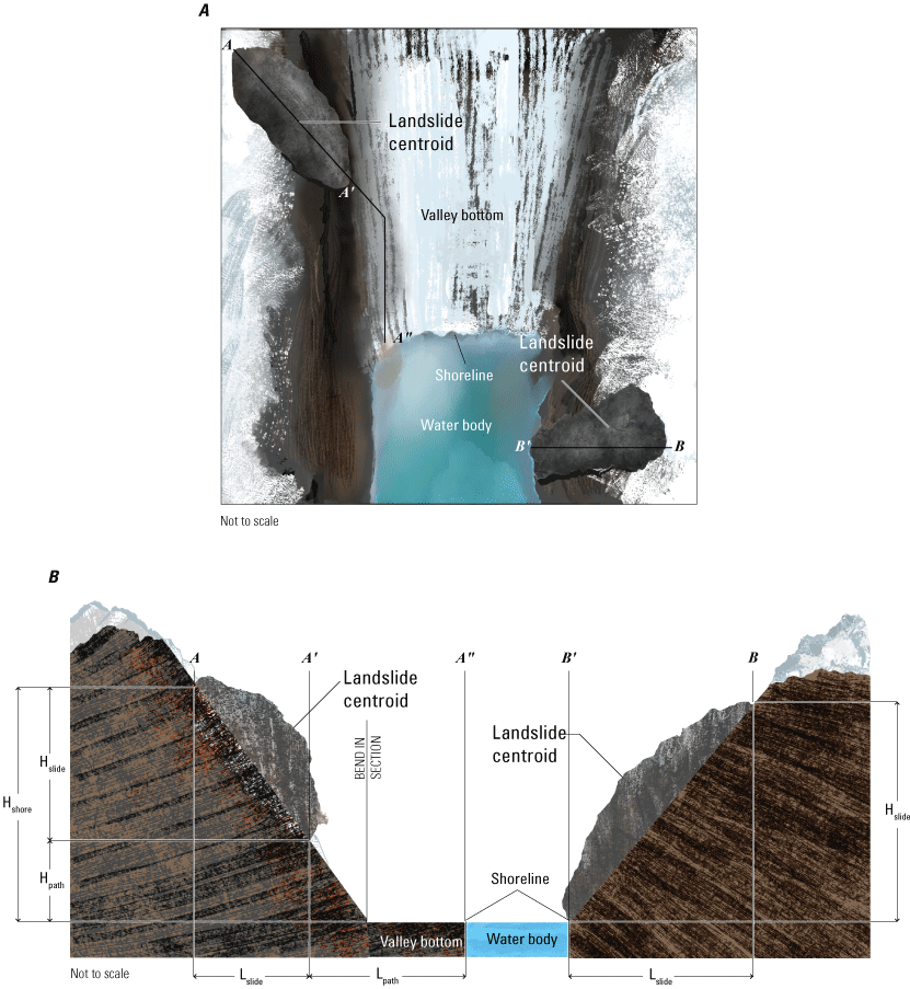
Conceptual diagram of the variables used to calculate the mobility required for the landslide to reach the nearest shoreline, Fshore, for the tsunami plausibility assessment. A, Map view and B, cross-sectional view of two possible topographic landslide configurations and their runout path for a landslide situated above a valley bottom (noted with A–A′–A”) and directly above a water body (noted with B–B′). For landslides not directly above water bodies, the distance (Lshore) and elevation difference (Hshore) of the landslide to the closest waterbody is the sum of the distance and elevation difference of the fall line (A–A′) and the length and elevation distance of the path from the bottom of the landslide to the shoreline (A′–A”).
Once the fall line direction, distance, and height were determined for the landslide polygon, we calculated the variables Hpath and Lpath along the path from the bottom of the landslide to the water body (A'–A” in figure 2). Here, we used an eight flow direction flow routing algorithm (Tarboton and others, 1997) to define the location of flow path from the bottom of the landslide to the nearest water body. Application of the algorithm on the original 5-m DEM resulted in an unnecessarily complex flowpath. Therefore, we iterated through several length-scale and smoothing parameter values and resampled the input DEM to 50-m and smoothed it using a mean filter within a circular neighborhood a length-scale (radius) of 10 pixels. These values preserved the broad-scale topographic influence on flow direction while reducing the unnecessary complexity of the defined flow path from the landslide to the nearest water body.
Inland water bodies included in this analysis were initially derived from the USGS National Hydrography Dataset Plus High-Resolution dataset (USGS, 2023). We include all waterbodies >0.5 km2 in our analysis. Coastal shorelines were defined using National Oceanic and Atmospheric Administration (NOAA) Center for Environmental Information Global Self-consistent, Hierarchical, High-resolution Geography Database (GSHHG) shorelines data (NOAA, 2023), which were manually revised to better reflect current shoreline locations in areas of rapid glacial recession or advancement in the study period (2016–22). We then calculated the values of Hpath and Lpath as the elevation difference (using the original 5-m DEM) and planimetric distance from A'–A” (fig. 2), where A” is located at the point at which the flowpath intersects the closest large waterbody (for example, a lake, fiord, or ocean). Fshore is then calculated as:
In the cases where the bottom of the landslide is located directly above a waterbody (for example, B–B' in fig. 2), it is not necessary to calculate a flowpath and instead define Fshore as Hslide / Lslide. The name of the nearest waterbody shoreline for each landslide is provided in table 1.1. Like mobility index F, Fshore is inversely related to landslide travel distance, where a low value of Fshore indicates a long travel distance and a high value of Fshore indicates a short travel distance. We then assigned a “plausible” tsunami potential rating to those landslides where Fshore is greater than or equal to F and an “implausible” tsunami potential rating for those landslides where Fshore is less than F. If any one of the three volumetric methods resulted in a plausible tsunami potential rating, we adopted a conservative approach and assigned the landslide as being plausibly tsunamigenic (refer to table 1.1). Again, this reflects the uncertainty in the area and volume calculations required for this analysis.
Results
Within our area of interest, we identified and confirmed 43 landslides, with variable sizes and velocities, that were moving between 2016 and 2022 (figs. 3–6, table 1). Of these, 14 landslides were previously documented (Dai and others, 2020; Coe and others, 2021; Higman and others, 2023; Schaefer and others, 2023), although they were not necessarily identified as moving in these earlier studies. Previously identified landslides are referred to by the names assigned by previous authors, and new landslides were named based on nearby geographic features. Landslides identified in this report occur throughout Prince William Sound but have a higher spatial density in the western portion of the study area (fig. 3). Landslides range in areal extent from 0.06 to 3.95 km2 and have minimum volumes ranging from 0.1 to 145×106 m3 and maximum volumes ranging from 0.92 to 1025×106 m3 (fig. 5, table 1, app. 1). Eighteen of the landslides are directly above present-day (as of April 2023) glacier termini, 28 are within 1 km of a glacier terminus, and 31 are within 2 km of a glacier terminus. For the snow-free months (June–October) in 2016 through 2022, average LOS speed (absolute value of velocity) ranged from 0.2 to 21 mm/yr, and peak LOS speed (absolute value of velocity) ranged from 5 to 41 mm/yr (table 1).
Of the 43 identified landslides, 11 have tsunamigenic plausibility if they failed catastrophically (depicted in blue, figs. 3 and 4; PSInSAR results for the 11 landslides are shown in fig. 6). Of these, three are directly above water (Barry Arm A, Yale D, and Yale E, fig. 6). The other eight are directly above glaciers or land with variable distance to the nearest waterbody. As described in the “Methods” section, tsunamigenic plausibility was calculated using three potential volumes: considering a small and large landslide mass with logarithmic spirals, and using V-A scaling. Of the 11 landslides, 5 landslides did not meet the criteria for tsunamigenic plausibility in one or more volume methods (Barry Arm B, Big Johnstone, Columbia, Portage A, and Yale F; app. 1). However, because one volume method did result in tsunamigenic plausibility, we chose a conservative approach and assigned it as having an overall rating of being tsunamigenically plausible. The smallest and largest calculated volumes considering all methods are shown in table 1, and all calculated volumes and their associated tsunamigenic plausibility estimates are provided in table 1.1.
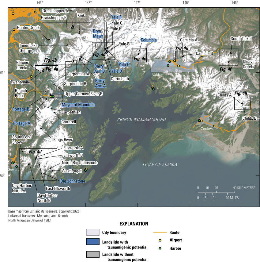
Location of landslides identified using persistent scatterer interferometric synthetic aperture radar. Black boxes show locations of figure 4 panels.
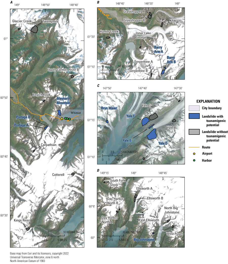
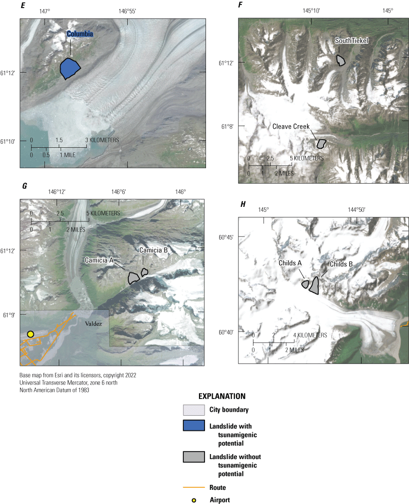
Details of landslides and landslide locations. Refer to figure 3 for locations of parts A–H within Prince William Sound.
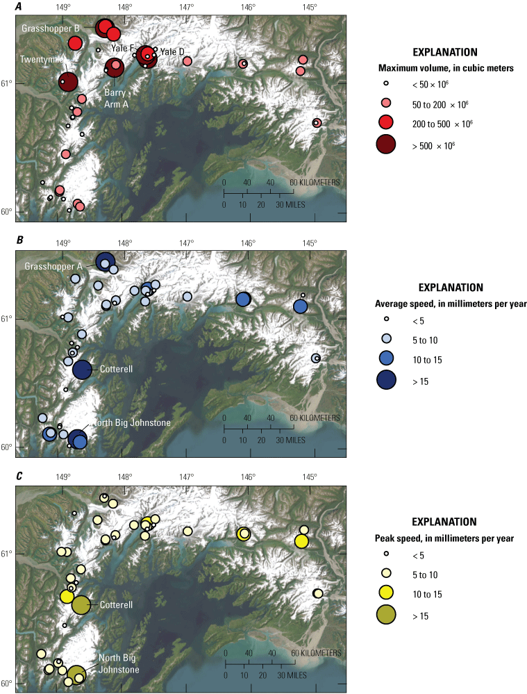
Landslide locations scaled as follows: A, maximum estimated volume, B, average line of sight (LOS) speed (absolute value of velocity) between 2016 and 2022, and C, peak LOS speed (absolute value of velocity) between 2016 and 2022. The landslides in each of the largest categories for each figure part (largest volume, fastest average speed, fastest peak speed for A, B, and C, respectively) are labeled.
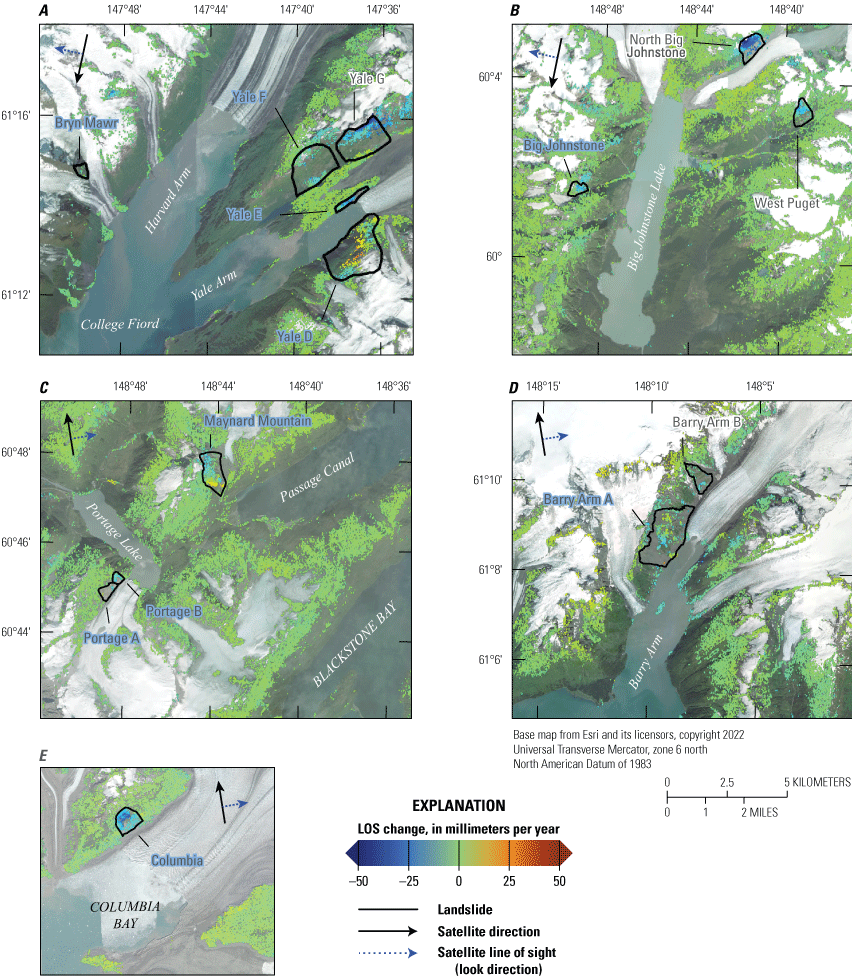
Example persistent scatterer interferometric synthetic aperture radar (PSInSAR) results for landslides with tsunamigenic plausibility. All deformation is in the line of sight (LOS) of the satellite look direction. Positive values indicate distances from the satellite to the ground surface became shorter (for example, vertical uplift or horizontal displacement in the direction of the sensor) and negative values indicate distances from the satellite to the ground surface became longer (for example, vertical subsidence or horizontal displacement away from the sensor). Most landslide areas are delineated based on PSInSAR points that show deformation, unless clear lineations associated with slope deformation were visible in imagery (for example, Yale F in Panel A), or the landslide has been previously delineated using high resolution imagery (for example, Barry Arm A and B in Panel D; Coe and others, 2021). Landslides with a blue label indicate those with tsunamigenic plausibility. Satellite path and analysis dates shown in the panels are as follows: A, P160, 2018–20; B, P160, 2018–20; C, P065, 2016–18; D, P065, 2016–18; E, P094, 2016–18.
Table 1.
List of deforming landslides, their characteristics, and the results of the preliminary tsunamigenic plausibility assessment.[Landslide volumes are the minimum and maximum determined from all three scenarios described in the “Methodology” section. Landslides with a plausible tsunamigenic potential are in bold font. Latitude and longitude are of the landslide centroid. Average and peak velocity values are for the summer months (June–October) between 2016 and 2021. DD, decimal degrees; WGS 84, World Geodetic System of 1984; km2, square kilometer; m3, cubic meter; x, multiplied by; LOS, line of sight; mm/yr, millimeters per year; =, equals]
Discussion
Our results identified 43 deforming landslides and established baseline rates of movement in the Prince William Sound region. Of the landslides that we identified, 29 were not previously recognized by optical analysis of imagery, emphasizing the complementary role that deformation mapping using radar remote sensing can play to more traditional mapping efforts, especially throughout large areas. Landslides identified in this report appear to occur primarily within bedrock as opposed to unconsolidated material, although field observations would be useful to verify this interpretation.
Landslide Inventory and Implications
The hazard associated with a possible tsunami likely varies substantially across landslides. Of the 43 deforming landslides, we identify 11 landslides that meet the defined mobility criteria for plausible tsunami generation. Landslide characteristics (for example, size, material properties, failure mechanism, runout behavior), waterbody type (for example, lake, fjord, open ocean), submarine characteristics (for example, water depth, submarine landforms), and landslide runout surface (for example, land, glacier ice, or direct entry into the water) all may affect the resulting tsunami characteristics (for example, wave height). However, a comparison based purely on size suggests that the inventory developed here contains two landslides with tsunamigenic potential (Yale D, Yale F; table 1, app. 1) that are of comparable size or larger than the Barry Arm A landslide, which has the potential to generate a hazardous wave of regional significance (Dai and others, 2020; Barnhart and others, 2021).
In comparing our landslide inventory to those in similar environments, such as Glacier Bay in Alaska (Kim and others, 2022), we find that the rates of landslide velocity are similar, on the order of 4 cm or less per year. These observed landslide velocities classify them as very slow (16 mm/yr to 1.6 m/yr) to extremely slow (less than 16 mm/yr) according to the International Geotechnical Society’s UNESCO Working Party on World Landslide Inventory (WP/WLI, 1995). Although average velocity is useful in defining destructive potential, it does not account for potential acceleration and the speed during catastrophic failure. Additionally, like in Glacier Bay, many of the landslides are near present-day (as of April 2023) glacier termini. Thus, landslide and landslide-generated tsunami hazards may continue to evolve as glaciers continue to thin and retreat.
Limitations
The data presented in this report are intended to provide a preliminary means of assessing rates of deformation within the study timeframe and to assess the potential hazard of the landslides identified using PSInSAR methods. Specifically, we use these results to identify landslides that show evidence of very slow to extremely slow movement and which may generate a tsunami should they fail catastrophically. The methods used for this analysis are not without limitation. An exhaustive compilation of all instabilities in the region, and confirmation of deforming areas as landslides, is challenging because of cloud and vegetation cover, poor lighting conditions, satellite imaging geometry, and the lack of high-resolution topography and bathymetry data. Most of the Prince William Sound region is covered in snow from November to May, which causes C-band Sentinel-1 InSAR observations to lose coherence. Additionally, much of the region is covered by moving glaciers, which cause decorrelation due to movement and melt processes, reducing the number of potential persistent scatterers. Moderately to rapidly moving landslides cannot be detected by InSAR observations because interferometric phases are constrained within 2π modulo (phase periodic with a 2π radian period). In other words, surface motion exceeding a half radar wavelength (for example, movement greater than about 2.8 centimeters between SAR datasets within a given pixel for the Sentinel-1 satellite) results in a large spatial gradient of phase changes and thereby loss of coherence (Lu and Kim, 2021). To correct unwrapped InSAR phase values, the phase variations between neighboring pixels should be less than π. This can result in a biased estimate of landslide velocity. Thus, the velocities presented herein are only accurate within the limits of the C-band PSInSAR method; for example, deformation measured using InSAR and pixel offset tracking of the Barry Arm A landslide indicates that the landslide was moving at a rate of 1–10 meters per year between 2016 and 2020 (Dai and others, 2020; Schaefer and others, 2023), which is not reflected in PSInSAR results herein. Other methods such as lidar differencing, longer-wavelength InSAR, or pixel offset tracking could provide more spatial measurements throughout a given landslide and thus provide a more accurate assessment of landslide velocities. The best methodological approaches for a given landslide is dependent on several landslide characteristics (for example, velocity, geometry, landslide type), which may be elucidated with further investigations. This additionally highlights the need for multi-sensor, multi-method approach for developing landslide inventories and their velocities in these regions.
The viewing geometry of the Sentinel-1 SAR satellite also causes displacement measurements to be affected by slope gradient, slope aspect, and geometric distortion (Natijne and others, 2022); north- and south-facing slopes have poor sensitivity because near-polar-orbiting SAR satellites are measuring distance from a right angle of satellite moving direction. Vegetation can further obscure C-band InSAR detection of landslides; longer-wavelength InSAR observations are more suitable for revealing landslides beneath vegetation and (or) snow cover (Lu and Kim, 2021; Xu and others, 2023). Thus, we consider this inventory to be more complete on vegetation- and snow-free slopes, and on east- and west-facing slopes.
Regardless of satellite orbit direction (ascending or descending track), coherence in the Prince William Sound region decreases with greater temporal separation between interferometric pairs. The number of high coherence points exceeding 0.3, which is often used as threshold of a reliable interferometric phase (Hanssen, 2001), is quickly reduced even during summer months, although multiples of a year (for example, 1, 2, 3, and so forth years for temporal baselines) tend to keep coherence because of the seasonal similarity in the area (fig. 7). Therefore, the dissipating coherence is a major obstacle in making timely, reliable InSAR measurements and identifying and monitoring landslides in this area.
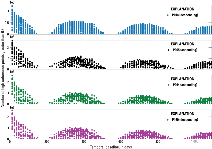
Number of high coherence (greater than [>] 0.3) points along temporal baselines (maximum: 3 years) of interferometric synthetic aperture pairs (look numbers are 18 [range] and 5 [azimuth], and coherence estimation windows are 3 in range by 3 in azimuth) from descending (P014, P160) and ascending (P065, P094) tracks.
The empirical nature of the V-A scaling and the mobility analysis results in uncertainty in the estimates of runout potential. Landslide volumes were estimated using V-A scaling and runout relations defined in other geographic, geologic, and climatic settings, which may significantly differ in lithology, structure, and origin. To ensure accurate size and volume estimates, more detailed analysis of the morphology and kinematics of the landslides included in this study is required. Additionally, estimates of landslide mobility required to reach the shoreline follow the shortest distance from the bottom of the landslide to the shoreline, which may not reflect the effect of topography (for example, intermediary ridgelines) on the potential travel path of a failed landslide. All mobility estimates are also based upon observed runout behavior of landslides on dry land. Landslides that run out on glaciers, of which there are several potential examples in this study, may exhibit runout characteristics that differ significantly from those forecasted using the methods included in this report (for example, Bottino and others, 2002). Specific analyses of the runout behavior of large rock avalanches in this environmental setting could better constrain the potential for catastrophic failures to enter the water and generate a tsunami.
Prioritizing Future Analyses
This report only depicts the plausibility of a given landslide entering a waterbody during catastrophic failure and makes no attempt to estimate the potential wave height, travel time, runup, inundation, current velocities, duration, or resonance of a landslide-generated tsunami. Additional modeling (for example, George and others, 2017; Barnhart and others, 2021) could be performed to better constrain the potential effect of a future catastrophic failure on communities, mariners, recreationalists, and the natural and cultural resources in, on, and around Prince William Sound. In addition, hazards presented by non-tsunamigenic landslides can be considerable, such as the potential for a landslide dam and subsequent dam-break flood. Persons traveling through, recreating, or performing commercial or subsistence activities should be aware of potential landslide hazards anytime in or below steep, potentially unstable terrain.
This report does not ascribe any likelihood to the catastrophic failure of these landslides. The determination of a likelihood or a probability estimate for any landslide is a difficult proposition. Slope stability and the potential for failure can be affected by many intrinsic and external factors, including material properties, weathering and alteration, changes in stress and strength conditions, hydrometeorological effects, and strong ground motion during a local or regional earthquake. In addition, catastrophic failure of a landslide is also possible without easily detectible precursory movement. Therefore, it must be assumed that landslide hazards are always present in the identified locations. Future investigations into the controls on slope stability, potential triggering conditions, material properties, geologic structure, and monitoring technologies may improve our understanding of the potential for catastrophic failure.
We conclude this discussion with a qualitative prioritization of the identified landslides for future analyses into “high,” “moderate,” and “low” categories (table 2). We assigned a “high” priority ranking to 11 landslides where a tsunami was determined to be a plausible outcome from rapid catastrophic failure because of the potential far-reaching nature of a tsunami. Within this category, landslides above connected water bodies may (for example, Yale D) may be expected to have farther-reaching effects than those above isolated water bodies (for example, Big Johnstone). However, because of boat traffic in these isolated water bodies and recreational activity along their shorelines, they remain in the “high” priority ranking. “Moderate” priorities were assigned to those landslides that did not meet the defined plausibility criteria but were (1) close to the numerical value defining plausibility (within 0.1), (2) proximal to known recreation areas, infrastructure, and (or) city boundaries, and (or) (3) have a glacier composing most of the runout surface which could increase runout travel distance. In addition to those 11 landslides identified as having tsunamigenic plausibility, we assigned a “moderate” priority to 6 landslides. The rationale for this assignment can be found in table 2. The remaining 26 landslides were assigned a “low” priority ranking for future analyses given the lack of known risk should these landslides fail catastrophically. It is important to note that further investigations may reveal characteristics of a given landslides that would modify these categories.
Table 2.
List of deforming landslides, the results of the preliminary tsunamigenic plausibility assessment, their priority for future analyses, and rationale for their priority ranking.[no. number; =, equals]
Conclusions
We used persistent scatterer interferometric synthetic aperture radar methods to determine areas that have exhibited deformation related to landslide processes from 2016 to 2022. We identified 43 landslides, 11 of which have the potential to generate a tsunami should they fail catastrophically. Given uncertainty in characterizing landslide size and runout potential, we ascribe a qualitative ranking of analyses priority to the identified landslides; the 11 landslides that met the tsunami plausibility criteria were considered to have a “high” priority for future analyses. Six additional landslides that were close to meeting the plausibility criteria or are proximal to city boundaries, infrastructure, or recreational areas were ascribed a “moderate” priority ranking.
Although the results presented herein represent a significant advancement in our understanding of the location and rate of landslide deformation in the Prince William Sound region, they should be considered preliminary and subject to revision. However, these data and results will contribute to improving our understanding of landslide and tsunami hazards in the region. The information presented here can be used to strategize future analyses, surveillance efforts, and hazard assessments for these newly identified landslides. Specifically, assessment of past landslide behavior, potential triggering conditions, and refined estimates of volume, mobility, and tsunamigenic potential could be prioritized for those landslides that have exhibited deformation in the persistent scatterer interferometric synthetic aperture radar analysis and have the potential to run out into the water or into developed areas or infrastructure.
Acknowledgments
We thank Jeffrey Coe, Paula Burgi, and Summer Ohlendorf for constructive reviews that helped to improve this manuscript.
References Cited
Alaska Division of Geological & Geophysical Surveys, 2023, Elevation portal: Alaska Division of Geological & Geophysical Surveys web page, accessed June 28, 2023, at https://elevation.alaska.gov/.
Allen, S.K., Gruber, S., and Owens, I.F., 2009, Exploring steep bedrock permafrost and its relationship with recent slope failures in the Southern Alps of New Zealand: Permafrost and Periglacial Processes, v. 20, no. 4, accessed April 1, 2023, at https://doi.org/10.1002/ppp.658.
Ballantyne, C.K., 2002, Paraglacial geomorphology: Quaternary Science Reviews, v. 21, no. 18–19, p. 1935–2017, accessed April 1, 2023, at https://doi.org/10.1016/S0277-3791(02)00005-7.
Barnhart, K.R., George, D.L., and Collins, A.L., 2023, digger—Utility tools for D-Claw: U.S. Geological Survey software release, accessed November 3, 2023, at https://doi.org/10.5066/P9EN7C2K.
Barnhart, K.R., Jones, R.P., George, D.L., Coe, J.A., and Staley, D.M., 2021, Preliminary assessment of the wave generating potential from landslides at Barry Arm, Prince William Sound, Alaska: U.S. Geological Survey Open-File Report 2021–1071, 28 p., accessed April 1, 2023, at https://doi.org/10.3133/ofr20211071.
Bessette-Kirton, E.K., and Coe, J.A., 2020, A 36-year record of rock avalanches in the Saint Elias Mountains of Alaska, with implications for future hazards: Frontiers in Earth Science, v. 8, article 293, 23 p., accessed April 1, 2023, at https://doi.org/10.3389/feart.2020.00293.
Blikra, L., Longva, O., Braathen, A., Anda, E., Dehls, J., and Stalsberg, K., 2006, Rock slope failures in Norwegian fjord areas—Examples, spatial distribution and temporal pattern in Evans, S.G., Mugnozza, G.S., Strom, A., and Hermanns, R.L., eds., Landslides from massive rock slope failure, v. 49 of NATO Science Series: Dordrecht, The Netherlands, Springer, p. 475–496, accessed April 1, 2023, at https://doi.org/10.1007/978-1-4020-4037-5_26.
Bottino, G., Chiarle, M., Joly, A., and Mortara, G., 2002, Modelling rock avalanches and their relation to permafrost degradation in glacial environments: Permafrost and periglacial processes, v. 13, no. 4, p. 283–288, accessed April 1, 2023, at https://doi.org/10.1002/ppp.432.
Coe, J.A., 2020, Bellwether sites for evaluating changes in landslide frequency and magnitude in cryospheric mountainous terrain—A call for systematic, long-term observations to decipher the impact of climate change: Landslides, v. 17, p. 2483–2501, accessed April 1, 2023, at https://doi.org/10.1007/s10346-020-01462-y.
Coe, J.A., Bessette-Kirton, E.K., and Geertsema, M., 2018, Increasing rock-avalanche size and mobility in Glacier Bay National Park and Preserve, Alaska detected from 1984 to 2016 Landsat imagery: Landslides, v. 15, no. 3, p. 393–407, accessed April 1, 2023, at https://doi.org/10.1007/s10346-017-0879-7.
Coe, J.A., Wolken, G.J., Daanen, R.P., and Schmitt, R.G., 2021, Map of landslide structures and kinematic elements at Barry Arm, Alaska in the summer of 2020: U.S. Geological Survey data release, accessed April 1, 2023, at https://doi.org/10.5066/P9EUCGJQ.
Dai, C., Higman, B., Lynett, P.J., Jacquemart, M., Howat, I.M., Liljedahl, A.K., Dufresne, A., Freymueller, J.T., Geertsema, M., Ward Jones, M., and Haeussler, P.J., 2020, Detection and assessment of a large and potentially tsunamigenic periglacial landslide in Barry Arm, Alaska: Geophysical Research Letters, v. 47, no. 22, article e2020GL089800, accessed April 1, 2023, at https://doi.org/10.1029/2020GL089800.
Duman, T.Y., Çan, T., Emre, Ö., Keçer, M., Doðan, A., Ates, S., and Durmaz, S., 2005, Landslide inventory of northwestern Anatolia, Turkey: Engineering Geology, v. 77, p. 99–114, accessed April 1, 2023, at https://doi.org/10.1016/j.enggeo.2004.08.005.
Fan, X., Yunus, A.P., Yang, Y.H., Subramanian, S.S., Zou, C., Dai, L., Dou, X., Narayana, C.A., Avtar, R., Xu, Q., and Huang, R., 2022, Imminent threat of rock-ice avalanches in high mountain Asia: Science of the Total Environment, v. 836, article 155380, accessed April 1, 2023, at https://doi.org/10.1016/j.scitotenv.2022.155380.
Ferretti, A., Prati, C., and Rocca, F., 2001, Permanent scatterers in SAR interferometry: IEEE Transaction on Geoscience and Remote Sensing, v. 39, p. 8–20, accessed April 1, 2023, at https://doi.org/10.1109/36.898661.
George, D.L., Iverson, R.M., and Cannon, C.M., 2017, New methodology for computing tsunami generation by subaerial landslides—Application to the 2015 Tyndall Glacier landslide, Alaska: Geophysical Research Letters, v. 44, no. 14, p. 7276–7284, accessed April 1, 2023, at https://doi.org/10.1002/2017GL074341.
Guzzetti, F., Carrara, A., Cardinali, M., and Reichenbach, P., 1999, Landslide hazard evaluation—A review of current techniques and their application in a multi-scale study, central Italy: Geomorphology, v. 31, nos. 1–4, p. 181–216, accessed April 1, 2023, at https://doi.org/10.1016/S0169-555X(99)00078-1.
Hanssen, R.F., 2001, Radar interferometry—Data interpretation and error analysis: Kluwer Acadamic Publishers, 308 p. [Also available at https://doi.org/10.1007/0-306-47633-9.]
Harbitz, C.B., Løvholt, F., and Bungum, H., 2014, Submarine landslide tsunamis—How extreme and how likely?: Natural Hazards, v. 72, p.1341–1374, accessed April 1, 2023, at https://doi.org/10.1007/s11069-013-0681-3.
Hermanns, R.L., Oppikofer, T., Anda, E., Blikra, L.H., Bohme, M., Bunkholt, H., Crosta, G.B., Dahle, H., Devoli, G., Fischer, L. and Jaboyedoff, M., 2013, Hazard and risk classification for large unstable rock slopes in Norway: Italian Journal of Engineering Geology and Environment, p. 245–254, accessed April 1, 2023, at https://doi.org/10.4408/IJEGE.2013-06.B-22.
Hermanns, R.L., Oppikofer, T., Anda, E., Blikra, L.H., Bohme, M., Bunkholt, H., Crosta, G.B., Dahle, H., Devoli, G., Fischer, L. and Jaboyedoff, M., Loew, S., Sætre, S., Yugsi Molina, F., 2012, Recommended hazard and risk classification system for large unstable rock slopes in Norway [NGU Report 2012.029]: Geological Survey of Norway.
Higman, B., Lahusen, S., Belair, G., Staley, D.M., and Jacquemart, M., 2023, Inventory of large slope instabilities, Prince William Sound, Alaska: U.S. Geological Survey data release, accessed October 26, 2023, at https://doi.org/10.5066/P9XGMHHP.
Higman, B., Shugar, D.H., Stark, C.P., Ekström, G., Koppes, M.N., Lynett, P., Dufresne, A., Haeussler, P.J., Geertsema, M., Gulick, S., Mattox, A., Venditti, J.G., Walton, M.A.L., McCall, N., Mckittrick, E., MacInnes, B., Bilderback, E.L., Tang, H., Willis, M.J., Richmond, B., Reece, R.S., Larsen, C., Olson, B., Capra, J., Ayca, A., Bloom, C., Williams, H., Bonno, D., Weiss, R., Keen, A., Skanavis, V., and Loso, M., 2018, The 2015 landslide and tsunami in Taan Fiord, Alaska: Scientific Reports, v. 8, article 12993, 12 p., accessed April 1, 2023, at https://doi.org/10.1038/s41598-018-30475-w.
Holm, K., Bovis, M., and Jakob, M., 2004, The landslide response of alpine basins to post-Little Ice Age glacial thinning and retreat in southwestern British Columbia: Geomorphology, v. 57, p. 201–216, accessed April 1, 2023, at https://doi.org/10.1016/S0169-555X(03)00103-X.
Hooper, A., 2008, A multi‐temporal InSAR method incorporating both persistent scatterer and small baseline approaches: Geophysical Research Letters, v. 35, no. 16, accessed April 1, 2023, at https://doi.org/10.1029/2008GL034654. https://doi.org/10.1029/2008GL034654
Hooper, A., Zebker, H., Segall, P., and Kampes, B., 2004, A new method for measuring deformation on volcanoes and other natural terrains using InSAR persistent scatterers: Geophysical Research Letters, v. 31, no. 23, accessed April 1, 2023, at https://doi.org/10.1029/2004GL021737.
International Geotechnical Society’s United Nations Educational, Scientific and Cultural Organization (UNESCO) Working Party on World Landslide Inventory [WP/WLI], 1995, A suggested method for describing the rate of movement of a landslide: Bulletin of the International Association of Engineering Geology, v. 52, p. 75–78, accessed April 1, 2023, at https://doi.org/10.1007/BF02602683.
Kim, J., Coe, J.A., Lu, Z., Avdievitch, N.N., and Hults, C.P., 2022, Spaceborne InSAR mapping of landslides and subsidence in rapidly deglaciating terrain, Glacier Bay National Park and Preserve and vicinity, Alaska and British Columbia: Remote Sensing of Environment, v. 281, article 113231, accessed April 1, 2023, at https://doi.org/10.1016/j.rse.2022.113231.
Klimeš, J., Novotný, J., Rapre, A.C., Balek, J., Zahradníček, P., Strozzi, T., Sana, H., Frey, H., René, M., Štěpánek, P., Meitner, J., and Junghardt, J., 2021, Paraglacial rock slope stability under changing environmental conditions, Safuna Lakes, Cordillera Blanca Peru: Frontiers Earth Science, v. 9, article 607277, accessed April 1, 2023, at https://doi.org/10.3389/feart.2021.607277.
Larsen, I.J., Montgomery, D.R., and Korup, O., 2010, Landslide erosion controlled by hillslope material: Nature Geoscience, v. 3, no. 4, p. 247–251, accessed April 1, 2023, at https://doi.org/10.1038/ngeo776.
Lu, Z., and Kim, J., 2021, A framework for studying hydrology-driven landslide hazards in northwestern US using satellite InSAR, precipitation and soil moisture observations—Early results and future directions: GeoHazards, v. 2, no. 2, p. 17–40, accessed April 1, 2023, at https://doi.org/10.3390/geohazards2020002.
Margielewski, W., 2006, Structural control and types of movements of rock mass in anisotropic rocks—Case studies in the Polish Flysch Carpathians: Geomorphology, v. 77, p. 47–68, accessed April 1, 2023, at https://doi.org/10.1016/j.geomorph.2006.01.003.01.003.
Maxar, 2023, Global enhanced GEOINT delivery: Maxar web page, accessed April 1, 2023, at https://evwhs.digitalglobe.com/myDigitalGlobe/.
McColl, S.T., 2012, Paraglacial rock-slope stability: Geomorphology, v. 153, p.1–16. [Also available at https://doi.org/10.1016/j.geomorph.2012.02.015.]
Natijne, A.L. van, Bogaard, T.A., van Leijen, F.J., Hanssen, R.F., and Lindenbergh, R.C., 2022, World-wide InSAR sensitivity index for landslide deformation tracking: International Journal of Applied Earth Observation and Geoinformation, v. 111, article 102829, accessed April 1, 2023, at https://doi.org/10.1016/j.jag.2022.102829.
National Oceanic and Atmospheric Administration [NOAA], 2023, A global self-consistent, hierarchical, high-resolution geography database (version 2.3.7): National Oceanic and Atmospheric Administration, accessed March 10, 2023, at https://www.soest.hawaii.edu/pwessel/gshhg/.
Nichol, J., and Wong, M.S., 2005, Satellite remote sensing for detailed landslide inventories using change detection and image fusion: International Journal of Remote Sensing, v. 26, no. 9, p. 1913–1926, accessed April 1, 2023, at https://doi.org/10.1080/01431160512331314047.
Penna, I.M., Magnin, F., Nicolet, P., Etzelmüller, B., Hermanns, R.L., Böhme, M., Kristensen, L., Nöel, F., Bredal, M., and Dehls, J.F., 2023, Permafrost controls the displacement rates of large unstable rock-slopes in subarctic environments: Global and Planetary Change, v. 220, article 104017, accessed April 1, 2023, at https://doi.org/10.1016/j.gloplacha.2022.104017.
Qu, F., Zhong, Q., Niu, Y., Lu, Z., Wang, S., Zhao, C., Zhu, W., Qu, W., and Yang, C., 2022, Mapping the recent vertical crustal deformation of the Weihe Basin (China) using Sentinel-1 and ALOS-2 ScanSAR imagery: Remote Sensing, v. 14, article 3182, 21 p., accessed April 1, 2023, at https://doi.org/10.3390/rs14133182.
Ramos-Bernal, R.N., Vázquez-Jiménez, R., Romero-Calcerrada, R., Arrogante-Funes, P., and Novillo, C.J., 2018, Evaluation of unsupervised change detection methods applied to landslide inventory mapping using ASTER imagery: Remote Sensing, v. 10, no. 12, article 1987, 24 p., accessed April 1, 2023, at https://doi.org/10.3390/rs10121987.
Schaefer, L.N., Coe, J.A., Godt, J.W., and Wolken, G.J., 2020, Interferometric synthetic aperture radar data from 2020 for landslides at Barry Arm Fjord, Alaska (ver. 1.4, November 13, 2020): U.S. Geological Survey data release, accessed April 1, 2023, at https://doi.org/10.5066/P9Z04LNK.
Schaefer, L.N., Coe, J.A., Wikstrom Jones, K., Collins, B., Staley, D.M., West, M., Karasozen, E., Miles, C., Wolken, G.J., Daanen, R.P., Baxstrom, K.W., 2023, Kinematic evolution of a large paraglacial landslide in the Barry Arm fjord of Alaska: Journal of Geophysical Research: Earth Surface, v. 128, no. 11, article e2023JF007119, accessed April 1, 2023, at https://doi.org/10.1029/2023jf007119.
Schaefer, L.N., Coe, J.A., and Wolken, G.J., 2022, Interferometric synthetic aperture radar data from 2021 for landslides at Barry Arm Fjord, Alaska: U.S. Geological Survey data release, accessed April 1, 2023, at https://doi.org/10.5066/P9QJ8IO4.
Scheidegger, A.E., 1973, On the prediction of the reach and velocity of catastrophic landslides: Rock Mechanics, v. 5, no. 4, p. 231–236, accessed April 1, 2023, at https://doi.org/10.1007/BF01301796.
Svennevig, K., Hermanns, R.L., Keiding, M., Binder, D., Citterio, M., Dahl-Jensen, T., Mertl, S., Sørensen, E.V., and Voss, P.H., 2022, A large frozen debris avalanche entraining warming permafrost ground—The June 2021 Assapaat landslide, West Greenland: Landslides, v. 19, p. 2549–2567, accessed April 1, 2023, at https://doi.org/10.1007/s10346-022-01922-7.
Tarboton, D.G., Bras, R.L., and Rodriguez-Iturbe, I., 1997, On the extraction of channel networks from digital elevation data: Hydrological Processes, v. 5, no. 1, p. 81–100, accessed April 1, 2023, at https://doi.org/10.1002/hyp.3360050107.
U.S. Geological Survey [USGS], 2023, National Hydography Plus High Resolution: U.S. Geological Survey webpage, accessed March 10, 2023, https://www.usgs.gov/national-hydrography/nhdplus-high-resolution.
Wilson, F.H., Hults, C.P., Mull, C.G, and Karl, S.M., comps., 2015, Geologic map of Alaska: U.S. Geological Survey Scientific Investigations Map 3340, 2 sheets, scale 1:1,584,000, 197-p. pamphlet, accessed April 1, 2023, at https://doi.org/10.3133/sim3340.
Xu, Y., Lu, Z., BurgmannR., Hensley, S., Fielding, E., and Kim, J.W., 2023, P-band SAR for ground deformation surveying—Advantages and challenges: Remote Sensing of Environment, v. 287, article 113474, accessed April 1, 2023, at https://doi.org/10.1016/j.rse.2023.113474.
Appendix 1. Tsunami Plausibility for Various Landslide Volume Methods
Table 1.1.
Calculated landslide mobility required to reach the shoreline (Fshore), and potential landslide mobility (F) and tsunami plausibility for the three considered landslide volume methods (logarithmic spiral—small, logarithmic spiral—large, and volume-area scaling power law).[no., number; m3, cubic meter; x, multiplied by; =, equals]
Conversion Factors
International System of Units to U.S. customary units
Publishing support provided by the Science Publishing Network,
Denver and Reston Publishing Service Centers
For more information concerning the research in this report, contact the
Center Director, USGS Geologic Hazards Science Center
Box 25046, Mail Stop 966
Denver, CO 80225
(303) 273-8579
Or visit Geologic Hazards Science Center website at
Disclaimers
Any use of trade, firm, or product names is for descriptive purposes only and does not imply endorsement by the U.S. Government.
Although this information product, for the most part, is in the public domain, it also may contain copyrighted materials as noted in the text. Permission to reproduce copyrighted items must be secured from the copyright owner.
Suggested Citation
Schaefer, L.N., Kim, J., Staley, D.M., Lu, Z., and Barnhart, K.R., 2024, Satellite interferometry landslide detection and preliminary tsunamigenic plausibility assessment in Prince William Sound, southcentral Alaska: U.S. Geological Survey Open-File Report 2023–1099, 22 p., https://doi.org/10.3133/ofr20231099.
ISSN: 2331-1258 (online)
Study Area
| Publication type | Report |
|---|---|
| Publication Subtype | USGS Numbered Series |
| Title | Satellite interferometry landslide detection and preliminary tsunamigenic plausibility assessment in Prince William Sound, southcentral Alaska |
| Series title | Open-File Report |
| Series number | 2023-1099 |
| DOI | 10.3133/ofr20231099 |
| Publication Date | January 24, 2024 |
| Year Published | 2024 |
| Language | English |
| Publisher | U.S. Geological Survey |
| Publisher location | Reston, VA |
| Contributing office(s) | Geologic Hazards Science Center, Volcano Science Center |
| Description | v, 22 p. |
| Country | United States |
| State | Alaska |
| Other Geospatial | Prince William Sound |
| Online Only (Y/N) | Y |