

Greater Sage-Grouse Habitat of Nevada and Northeastern California—Integrating Space Use, Habitat Selection, and Survival Indices to Guide Areas for Habitat Management
Links
- Document: Report (8 MB pdf) , HTML , XML
- Data Release: USGS Data Release - Rasters representing Greater sage-grouse space use, habitat selection, and survival to inform habitat management
- Download citation as: RIS | Dublin Core
Acknowledgments
We thank the countless biologists and technicians who captured and tracked radio-marked sage-grouse, especially M. Atamian, E. Blomberg, D. Gibson (University of Nevada, Reno [UNR]); D. Davis (University of Idaho); Z. Lockyer, J. Dudko, S. Mathews, I. Dudley (Idaho State University); E. Tyrell, B. Prochazka (University of California, Davis). Critical geographic information system and administrative support were expertly provided by C. Weise, L. Parker, K. Bollens, E. Sanchez-Chioptea, (U.S. Geological Survey-Western Ecological Research Center [USGS-WERC]). We appreciate the efforts of J. Atkinson (USGS-WERC) for assisting with report preparation; and D. Nahhas and R. Obstaculo (Sacramento Publishing Service Center) for editing, formatting, and final production of this report. We thank K. McGowan (Nevada State Sagebrush Ecosystem Technical Team) and all members of the Nevada State Sagebrush Ecosystem Council. J. Tull (U.S. Fish and Wildlife Service [USFWS]), G. Wann (USGS-Fort Collins Science Center), T. Kimball, K. Miles (USGS-WERC) provided constructive comments on previous draft reports, as well as members of the Sagebrush Ecosystem Council, particularly J. Tibbitts (Eureka County) and J. Drew (Resource Concepts, Inc.). We thank S. Abele (USFWS), P. Deibert, J. Sedinger (UNR), and S. Espinosa (Nevada Department of Wildlife [NDOW]) who served as part of an expert review team that periodically provided feedback on this project. We thank Ormat Technologies, Inc., LS Power, and Midway Gold Corp. This work was funded by Nevada and California Bureau of Land Management and State of Nevada Sagebrush Ecosystem Program and represents a collaborative effort between USGS-WERC, NDOW, California Department of Fish and Wildlife, and Bureau of Land Management.
Preface
This study was done to provide scientific findings to help inform habitat maps for greater sage-grouse (Centrocercus urophasianus) in Nevada and northeastern California. Specifically, we provide these analyses to help inform the Bureau of Land Management’s (BLM) land use planning amendment and associated environmental impact statements (86 FR 66331). These findings provide updated, detailed, and comprehensive information about the status of habitat for this species of high conservation concern in Nevada and California. Importantly, this document provides an example of integrating indices of habitat selection and survival during different life stages and seasons with updated indices on current occupancy patterns to delineate specific example habitat management categories that can be used by the BLM and other land managers to inform decisions related to conservation and management.
Executive Summary
Greater sage-grouse populations (Centrocercus urophasianus; hereafter sage-grouse) are threatened by a suite of disturbances and anthropogenic factors that have contributed to a net loss of sagebrush-dominant shrub cover in recent decades. Declines in sage-grouse populations are largely linked to habitat loss across their range. A key component of conservation and land use planning efforts for sage-grouse involves the continued monitoring and modeling of habitat requirements and suitability across its range. The Bureau of Land Management (BLM) is addressing the management of sage-grouse habitats on BLM-authorized public lands throughout the western United States through a land use planning amendment and associated environmental impact statement (86 FR 66331). More than 25 percent of the range-wide distribution of sage-grouse is within Nevada and northeastern California, and information on sage-grouse distribution and habitat requirements is important to guide appropriate management decisions. Therefore, the BLM has identified the need for updated spatially explicit information on sage-grouse habitat in Nevada and northeastern California to guide the land use planning amendment and associated management decisions.
To address this need, researchers with the U.S. Geological Survey, in close cooperation with multiple State and Federal resource agency partners, including BLM, Nevada Department of Wildlife (NDOW) and California Department of Fish and Wildlife (CDFW), sought to map sage-grouse distribution and produce example habitat designations in these states. Herein, we report results of our primary study objective, which was to map sage-grouse habitat and create example habitat management areas, based on more than a decade of location and survival data collected from marked sage-grouse across the study region coupled with lek count survey data managed by the NDOW and the CDFW.
We expanded on previously developed methodology to incorporate information on habitat selection and survival during reproductive life stages and specific seasons with updated sage-grouse location and known fate datasets, while also including brood-rearing areas that are understood to be threatened and important for population persistence. We combined predictive habitat map surfaces for each life stage and season with updated information on current occupancy patterns to classify habitat based on its suitability and probability of occupancy. We carried out additional steps to delineate specific example habitat management areas, specifically (1) incorporated corridors connecting key nesting and brood-rearing habitat, (2) corrected outputs for pre-wildfire habitat conditions within areas burned in the last 16 years, and (3) masked out areas of anthropogenic development. Our methodological example of deriving habitat management areas was intended to help inform decisions by BLM and other land managers regarding conservation and management of sage-grouse. Associated data products in the form of habitat maps provide updated, detailed, and comprehensive information about the status of habitats and can be useful to partner agencies in their efforts to designate and rank habitats for this species of high conservation concern in Nevada and California, with full recognition that on-the-ground field data and local sources of information and expertise should be used in conjunction with inferences from these models.
Background
Western North American sagebrush (Artemisia spp.) ecosystems are threatened by a suite of disturbances and anthropogenic factors that have contributed to a net loss of sagebrush-dominant shrub cover throughout recent decades. Threats and disturbances to sagebrush ecosystems have been described thoroughly in scientific literature, and include climate change, severe drought, altered wildfire regimes, expansion of native and non-native plant and wildlife species, anthropogenic development, and land use change (Miller and Rose, 1999; Andreadis and Lettenmaier, 2006; Seager and others, 2007; Leu and others, 2008; Boyd and others, 2017; Davies and Bates, 2017; Heinrichs and others, 2018; Coates and others, 2021a; Harju and others, 2022). Changes in sagebrush ecosystems have preceded corresponding negative population trends for sagebrush obligate species, such as greater sage-grouse (Centrocercus urophasianus, hereafter sage-grouse; Connelly and Braun, 1997; Knick and others, 2011; Coates and others, 2021b), leading to large-scale efforts to curb declines and prevent the continued loss of sage-grouse habitat and habitat for other shrub- and grassland-dependent species within the sagebrush biome (Bureau of Land Management, 2015; Stiver and others, 2015). Because declines in sage-grouse populations are largely linked to habitat loss, a key component of conservation efforts for the species involves the continued monitoring and modeling of habitat requirements and suitability across its range to inform land use management plans (Coates and others, 2016b, 2020a; O’Neil and others, 2020; Brussee and others, 2022; Saher and others, 2022; Wann and others, 2023).
Under the National Environmental Policy Act of 1969, as amended, and Federal Land Policy and Management Act of 1976, as amended, the Bureau of Land Management (BLM) is required to develop resource management plans to guide management of public lands and to keep the plans current through amendments or revisions, as needed. The BLM is responsible for management of sagebrush ecosystems and sage-grouse habitat on BLM-authorized public lands throughout the western United States through a land use planning amendment and associated environmental impact statements (86 FR 66331; Bureau of Land Management, 2021). Amended plans will update sage-grouse and sagebrush management strategies that were most recently finalized in 2015 and 2019. The goals of this land use planning initiative include improving land management-related decisions to be consistent with new science by addressing rapid changes affecting sagebrush ecosystems, which include loss of sagebrush, invasion of annual grasses, severe drought, contemporary wildfire regimes, and loss of riparian areas. As part of this initiative and associated revisions, each of the western states were given an opportunity to update habitat designations and maps for sage-grouse populations based on best and current available science. The Nevada Department of Wildlife, California Department of Fish and Wildlife, and BLM have previously partnered with the U.S. Geological Survey (USGS) to map sage-grouse habitat in these states. However, previous maps were based on seasonal habitat selection patterns and indices of space use (Coates and others, 2016b, 2020a) that did not include information on survival across different life stages. More recent methodological advancements have incorporated survival information into the mapping process (O’Neil and others, 2020; Brussee and others, 2022). In addition, the USGS has continued to monitor sage-grouse populations within Nevada and northeastern California, while adding new populations for monitoring, providing an opportunity to improve and update data-driven models that quantify and map habitat suitability (Smith and others, 2014; Kirol and others, 2015). Here, we build on previously developed methodology to incorporate information on selection and survival during different reproductive life stages (nest and brood survival) and specific seasons, while building in methods that ensure inclusion of brood-rearing areas that are understood to be at risk and important for population persistence.
Habitat modeling for sage-grouse, and many other avian species, has been conventionally carried out by analytically contrasting known locations of individual birds relative to random locations that characterize availability. These data, and subsequent analyses, have been referred to as “use versus availability” designs (Pearce and Boyce, 2006; McDonald, 2013; Warton and Aarts, 2013), and models used to analyze the data most commonly are referred to as “species distribution models,” “habitat selection models,” or “resource selection functions” (Johnson and others, 2006; Phillips and Dudik, 2008; McDonald, 2013; Matthiopoulos and others, 2015; Renner and others, 2015). The analytical methods used to fit such models vary widely depending on the level of complexity needed or desired by the analysts, but the foundational statistical framework for most of these applications has been demonstrated to be mathematically analogous to an inhomogeneous Poisson spatial point process (Warton and Shepherd, 2010; Aarts and others, 2012; Warton and Aarts, 2013). Applications of species distribution and habitat selection models are widespread in the literature and are especially useful for describing and mapping spatial patterns in distribution and the primary environmental correlates of this distribution (Elith and others, 2006; Matthiopoulos and others, 2015; Renner and others, 2015). However, a weakness of all analyses that rely solely on location data is that species performance (survival, reproduction, and population change) cannot be directly estimated.
Importantly, many species’ distributions and habitat selection patterns do not perfectly align with positive performance (for example, negative population rate of change in abundance), implying that not all occupied habitats should be considered suitable. Although there are a variety of explanations for why populations might occupy suboptimal habitat (Van Horne, 1983; Battin, 2004; Robertson and Hutto, 2006; Hirzel and Le Lay, 2008; Hale and Swearer, 2017), one contemporary reasoning is that rapidly changing environments, characteristic of the Anthropocene, can outpace the evolutionary capacity of native species to adapt (Merkle and others, 2022; Ravi and others, 2022). Under these conditions, species with strong selective patterns of site fidelity are the most vulnerable to changes that might happen on relatively rapid time scales (Merkle and others, 2022). The sage-grouse is a textbook example of a species demonstrating these traits in an environment undergoing rapid transition. Sage-grouse are known to return to previous breeding grounds and nest sites (Holloran and Anderson, 2005; O’Neil and others, 2020), and the habitats they occupy are increasingly altered by wildfire, annual grass invasion, loss of mesic habitat productivity resulting from drought or weather pattern changes, and anthropogenic development (Coates and others, 2016c; Foster and others, 2019; O’Neil and others, 2020; Anthony and others, 2021; Brussee and others, 2022). Sage-grouse occupancy of increasingly fragmented habitat is often expected to manifest in source-sink landscape population dynamics characterized by the presence of ecological traps (Battin, 2004) and maladaptive habitat selection (Heinrichs and others, 2018; Cutting and others, 2019; Pratt and Beck, 2021; Brussee and others, 2022).
Because of this potential maladaptive selection, whenever possible, delineations of habitat for species of conservation interest, such as sage-grouse, will benefit from quantifying performance within the boundaries of selected habitat where habitat suitability is measured in terms of success within selected habitat instead of gradients of selection/occupancy alone (Hirzel and Le Lay, 2008; Gaillard and others, 2010; Matthiopoulos and others, 2015). The outcomes of such exercises can be critical toward identifying threatened priority habitats and determining the need for restoration after disturbance (Pyke and others, 2020; Saher and others, 2022). For example, the loss of habitat and subsequent restoration potential can be characterized not only by previous distribution and habitat use, but by the expected loss of success due to continued occupation of degraded habitat (Roth and others, 2022).
An additional consideration when implementing comprehensive approaches to habitat suitability and species distribution modeling is the concept of seasonal and life stage-specific responses, wherein certain life stages may be especially important or indicate limitations that have disproportionate implications for overall population growth and stability. Sage-grouse and many other species rely on seasonal migrations within an annual home range to meet the habitat needs of specific life stages. For example, sage-grouse often move to higher elevations when raising broods to access more productive vegetation typically associated with late-season moisture availability (Drut and others, 1994; Donnelly and others, 2016, 2018) but later move to lower elevations and southern exposures during winter to gain better access to sagebrush forage (Connelly and others, 2000). Consequently, habitat analyses may require a seasonal or life stage-specific focus to identify key source areas (for example, relatively high selection and increased reproductive performance) and sink (high selection with reduced performance) areas that may disproportionately affect populations during critical life stages. Such characteristics are more likely to go undetected when considering population response within an annual home range or time step. Furthermore, because reproductive performance is expected to be a primary determinant of population growth, analyses may benefit from partitioning responses between males and females within the population.
Finally, when identifying habitat suitability, the distribution of current occupancy should be considered if objectives include mapping the true or realized species distribution. Because habitat selection and species distribution analyses involve predictive models, mapping habitat does not inherently account for areas that consist of conditions that are consistent with occupied, selected habitat, but are not occupied for reasons independent of habitat suitability. In most ecological studies, proxies for abundance and space use are evaluated separately from measures of habitat selection or quality, independently informing conservation and management decisions (Stephens and others, 2015). However, coarse data on current occupancy patterns can be combined with fine-scale data on habitat suitability to guide landscape-scale management decisions (for example, Coates and others, 2016b, 2020a). This combination can highlight priority areas for habitat preservation, identify areas where management and restoration activities are likely to have the greatest benefit, identify areas where anthropogenic development can occur with minimal effects, and indicate regions where reintroduction or translocation might be appropriate.
Objectives
Nevada and northeastern California contain a substantial proportion of the present-day range-wide distribution of sage-grouse (Coates and others, 2021b). To provide information necessary for management decisions, including BLM’s land use planning amendment and associated environmental impact statements (86 FR 66331), our primary objective was to map sage-grouse habitat and produce example habitat management areas in these states. To produce this map, we investigated habitat responses by sage-grouse in Nevada and northeastern California, using a comprehensive research study design, wherein habitat selection and survival patterns were considered and mapped across six distinct annual life stages and seasons: (1) nesting, (2) early brood-rearing, (3) late brood-rearing, (4) spring, (5) summer, and (6) winter. The overarching goal was to establish example habitat management areas that may be used by the BLM and other land managers to guide conservation and management decision-making in conjunction with on-the-ground field data and local expertise. The specific objectives were:
-
1. Evaluate habitat selection patterns across six distinct annual life stages and seasons to generate predictive habitat map surfaces.
-
2. Evaluate survival patterns across three reproductive life stages to produce predictive habitat map surfaces.
-
3. Model and map space use and occupancy.
-
4. Integrate indices of selection and survival with those of occupancy to delineate example habitat management areas.
Study Area
We collected data at 15 field sites within the northern Great Basin region during 2009–21 (fig. 1). Northern and western sites were typical sagebrush steppe and generally received more precipitation relative to other sites, whereas south-central sites consisted of warmer and drier soil types of sagebrush semi-desert (West and Young, 2000). Elevations among study areas ranged from 1,158 to 3,770 meters (m). At high elevations, mountain big sagebrush (Artemisia tridentata ssp. vaseyana) was common, whereas lower elevations (below 2,100 m) primarily consisted of Wyoming big sagebrush (Artemisia tridentata ssp. wyomingensis), black (Artemisia nova), and low (Artemisia arbuscula) sagebrush. Non-sagebrush shrubs included rabbitbrush (Chrysothamnus ssp.), Mormon tea (Ephedra viridis), snowberry (Symphoricarpos spp.), western serviceberry (Amelanchier alnifolia), and antelope bitterbrush (Purshia tridentata). Conifer forests were most frequently composed of single-leaf pinyon pine (Pinus monophylla) and Utah juniper (Juniperus osteosperma; hereinafter, pinyon-juniper). Herbaceous vegetation consisted of non-native annual grasses, including cheatgrass (Bromus tectorum) and medusahead rye (Taeniatherum caput-medusae) and native perennial grasses, including needle and thread (Hesperostipa comata), Indian ricegrass (Achnatherum hymenoides), and squirreltail (Elymus elymoides).
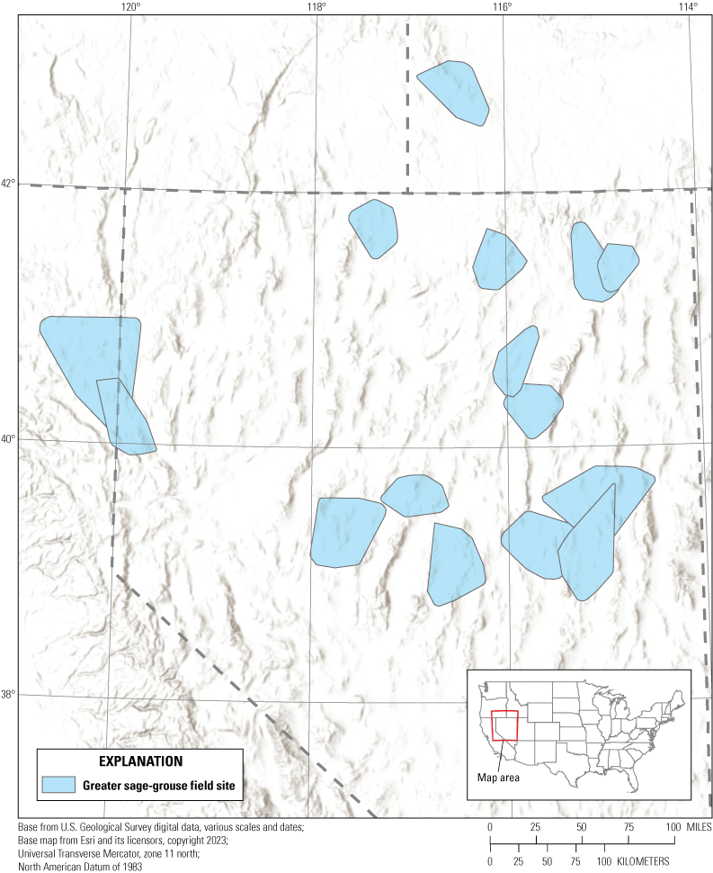
Field sites in the western Great Basin region where greater sage-grouse (Centrocercus urophasianus) were monitored from 2009 to 2021.
Methods
We captured sage-grouse at night using spotlighting techniques (Giesen and others, 1982; Wakkinen and others, 1992). We outfitted sage-grouse with necklace-style very high frequency (VHF) radio-transmitters (Kolada and others, 2009), and for a subset, we included combined rump-mounted Global Positioning Systems (GPS)—Platform Transmitter Terminals (North Star Science and Technology, LLC, King George, Virginia). During the nesting period, hens were tracked every 3 days until nests hatched or failed as determined by either a visual assessment of eggshell remains or observing chicks in the nest bowl. During the brood-rearing period, broods affiliated with marked females were located every 10 days for as many as 50 days during daylight or nocturnal hours. Nocturnal checks consisted of using spotlighting to confirm presence or absence of chicks. We only used GPS location data for winter analyses because location frequency collected from VHF transmitters was inadequate during this period. All sage-grouse were captured and handled in accordance with USGS Western Ecological Research Center Animal Care and Use Protocol WERC-2015-02.
Environmental Landscape Covariates
We quantified landscape conditions potentially associated with sage-grouse habitat using remotely sensed geographic information system (GIS) products. Landscape conditions included vegetation type, hydrologic features, and topography. We considered all landscape variables at multiple spatial scales (Aldridge and others, 2008; Casazza and others, 2011) calculated from sage-grouse movement patterns. We calculated landscape characteristics using a circular moving window (neighborhood analysis tool, ArcGIS Spatial Analyst) within radii representing the minimum (167.9 m; 8.7 hectare [ha]), mean (439.5 m; 61.5 ha), and maximum (1,451.7 m; 661.4 ha), daily distances traveled by sage-grouse primarily during the spring and summer seasons (Coates and others, 2016b). We also included neighborhoods corresponding to 75, 260 and 370 m for nest and brood analyses based on the assumption that movement patterns would be different during these life stages because a female is tied to either a single nest site or a brood that has limited mobility (Dudko and others, 2018). The smallest radius (75 m; 1.8 ha) was intended to accommodate landscape attributes more directly associated with cover characteristics at sage-grouse nest locations.
To characterize shrubland cover types, we used Rangeland Condition Monitoring Assessment and Projection base layers from the National Land Cover Database (RCMAP; Rigge and others, 2020), where each 900-square meter (m2) pixel represented a continuous percentage of cover. Vegetation cover types included annual percent cover of sagebrush, non-sagebrush shrub, and total shrub cover. We used Rangeland Analysis Platform data (RAP; Jones and others, 2018; Allred and others, 2021) to characterize annual estimates of percent cover of bare ground, annual grass, perennial grass, litter, total shrub, and tree cover. We used data from the Sage Grouse Initiative representing mesic areas (Donnelly and others, 2016) to extract alfalfa fields. To characterize burned areas, we created spatiotemporal surfaces of cumulative burned area using Monitoring Trends in Burn Severity (U.S. Geological Survey, 2020) data combined with information on sagebrush recovery rates (Coates and others, 2016c; O’Neil and others, 2020). We included an interaction between annual grass and burned areas in summer selection, brood selection, and brood survival models to account for varying responses to annual grass and recent burns previously documented during key brood-rearing periods (Brussee and others, 2022). Hydrologic feature representations included combined intermittent and perennial stream types, and perennial streams only, which were gathered from the National Hydrography Dataset (U.S. Geological Survey, 2017). We obtained data representing wet meadow and riparian features from the U.S. Fish and Wildlife Service National Wetlands Inventory (https://www.fws.gov/program/national-wetlands-inventory/wetlands-data). We measured distances to hydrologic, wetland, and alfalfa features using Spatial Analyst (ArcGIS 10.6.1). We transformed all distance-based variables so their effects would decay with increasing distances using the formula exp(−d/α), where α represented either the median distance value measured from all locations, or 1,451 m (maximum daily distance traveled), whichever was smaller. For alfalfa, we also considered log-transformed distance to account for the potential for human-modified landscapes to affect sage-grouse beyond 1,451 m, primarily by affecting the predator community (Coates and others, 2016a, 2020b). We also calculated density of linear and polygon features (streams and alfalfa fields) within each moving window scale. Topographic variables derived from digital elevation models (900-m2 pixels) included elevation, topographic roughness representing variance in elevation (Riley and others, 1999; Evans and others, 2014), topographic position index (TPI; De Reu and others, 2013), heat load index (HLI; McCune and Keon, 2002), and transformed aspect (TRASP; Roberts and Cooper, 1989). We averaged each of these indices across each circular moving neighborhood to capture scale-dependent responses.
Study Design
To evaluate sage-grouse use of the landscape relative to all accessible habitat, we characterized available habitat in GIS by generating five random locations for each used location for each life stage and season (Northrup and others, 2013). For nests and broods, we calculated the 95th percentile of distance from used locations to the nearest lek (for analysis of nest data) and to nests (for analysis of brood data) separately for each study site. Using these distances, we created buffers around leks and nests within which we then conditioned the available distribution of background locations (Holloran and Anderson, 2005; Coates and others, 2013). We defined spring as March 16–June 30, summer as July 1–October 15, and winter as October 16–March 15. For seasonal models, we restricted available locations to within the 99-percent kernel utilization distribution (UD) using all locations from each study site for a given season to delineate each boundary. We generated five random locations for every used location with the boundary. We extracted values of landscape vegetation characteristics, distance metrics, and topographic indices at used and random locations for all analyses. We centered and standardized continuous landscape variables that represented index values or percent cover and centered exponential decay variables.
Sage-grouse require specific vegetation components during brood-rearing which are functionally different from those required for nesting. When the two habitat types are not adjacent, females must move their broods to meet the requirements of this later reproductive life stage. For these reasons, we classified vegetation characteristics used during the transitional period (defined as 20 days after hatch) as early brood-rearing habitat, whereas those used from days 21 to 51 post hatch were classified as late brood-rearing habitat. We performed our analyses separately for early and late brood-rearing stages (Blomberg and others, 2013; Brussee and others 2022).
For all analyses, we withheld 15 percent of all birds and reserved it to use as testing data for model validation. The data from the remaining 85 percent of birds was used to train models and predict habitat. Model validation techniques are described in the following sections and were used to check model fit and predictive capacity of all final models across seasons and life stages.
Analysis: Variable Selection
In total, we considered 90 landscape variables as candidates in our models for selection and survival. However, we could not fit models to the complete dataset because we measured similar habitat characteristics across multiple spatial scales; strong pairwise correlations existed between some of these covariates (|r|>0.65), and model performance suffers when large numbers of covariates are used to predict a response, resulting in overfitting (Tibshirani and others, 2012; Dormann and others, 2013). To consider all candidate variables equally while accounting for these potential issues, we implemented Bayesian variable and scale selection techniques to evaluate statistical support for each variable and scale and subsequently identify a subset of the most predictive variables to be used for habitat mapping.
Our variable and scale selection models combined two methodological approaches to first identify the most effective variable among a group of similar and typically correlated variables and second to test statistical support for inclusion of those variables when included in models with subsets of other potentially important variables. The first method, known as Bayesian latent indicator scale selection (BLISS; Stuber and others, 2017), was specified to identify the most appropriate scale within a group of candidate scales. Briefly, the BLISS method facilitates estimation of a latent categorical probability for each variable within a defined group. For example, given six measurements of sagebrush cover at six different scales, BLISS estimates a posterior probability (0–1) for each scale. The highest probability can then be interpreted as the scale with the most statistical support (Brussee and others, 2022; O’Neil and others, 2023). The second method, known as Gibbs or indicator variable selection (Kuo and Mallick, 1998; O’Hara and Sillanpää, 2009), involves specifying an indicator dummy variable, termed “w,” to be assigned to each candidate variable (or each group of candidate variables). When fit using Markov Chain Monte Carlo (MCMC) sampling methods, the inclusion probability for each variable is updated, and the support for inclusion can be evaluated from the proportion of MCMC iterations where w=1. Hierarchical modeling using MCMC sampling methods allows BLISS and indicator variable selection to be incorporated within the same model framework, such that the probability of inclusion for all candidate variables could be evaluated from Bayesian posterior distributions. We assigned flat priors for sub-variables within groups (as in, equal prior probability of selection for each scale) and assigned a prior probability of 0.5 for each w, representing a 50/50 initial probability of inclusion. We fit models using MCMC procedures described in proceeding sections (“Analysis: Computation”) and carried forward the variables receiving substantial statistical support when fitting a final predictive model for each season and life stage. Final variables were included if w was greater than 0.50 from the highest supported scale for each candidate group.
Analysis: Models for Habitat Selection
For each life stage and season, we analyzed habitat selection by contrasting used locations with random available locations (Johnson and others, 2006; Northrup and others, 2013) to infer sage-grouse spatial habitat patterns. Specifically, the base model took the form shown in equation 1:
whereβ0
is the fixed effects intercept,
Xβ
is a vector of selection coefficients multiplied by the matrix of fixed environmental covariates, and
γ and η
are random effects for year and individual bird to account for multiple observations drawn from each bird and to balance the study throughout the course of each life stage, respectively (Gillies and others, 2006).
The response observations Y were assumed to follow a Bernoulli distribution, with y=1 indicating a sage-grouse location, and y=0 indicating a randomly sampled background location. After estimation of all model parameters, we computed the resource selection function, , by discarding the intercepts and applying the exponential link: (Johnson and others, 2006; McDonald, 2013; Northrup and others, 2013). We validated our models by applying resource selection function (RSF) cross-validation methods to the independent testing data subset. We interpreted each model’s ability to make predictions proportional to the probability of selection from linear model fit statistics (β, R2, Spearman’s rank coefficient ρ), comparing the proportion of observations in the testing dataset to those expected based on ordinal RSF bins from the fitted model (Johnson and others, 2006; Fieberg and others, 2018). Full model specification is reported in appendix 1.
Analysis: Models for Survival
We used a hierarchical logistic exposure model (Rotella and others, 2004; Shaffer, 2004; Catlin and others, 2015) to estimate survival across all life stages and evaluate habitat covariate effects. The logistic exposure model assumes a daily survival rate (DSR) that follows a Bernoulli distribution, wherein each day the event of interest represented whether the nest or brood survived. Exposure time is accounted for through the length of each encounter history. For each life stage, we created encounter histories for each bird that consisted of known alive and censored intervals throughout the season. For nests and broods, encounter histories ended with either a successful or failed nest (or brood), and exposure time was calculated as the length of time between visits. To model environmental effects, we considered only the landscape covariates that were determined to be important in the variable and scale selection process. For brood models, we created two time-varying categorical brood stage variables representing early versus late. Because it was not always possible to perform counts exactly 10 days apart, when time intervals overlapped both periods, we split the encounter history and divided the exposure time to correspond to each brood age. When broods failed during an interval that overlapped 21 days for brood age, we allowed the covariate information to inform effects for early and late broods (Brussee and others, 2022). For example, for early broods, the categorical brood stage multiplier variable was 0 for late brood intervals, thus only covariates determined to be important for early brood survival varied, whereas variables determined to be important for survival of late broods were held constant at 0. Similar to the base model for habitat selection, DSR was modeled through the logit link function shown in equation 2:
whereγ0
is a baseline intercept,
Xβ
is a vector of coefficients multiplied by the matrix of fixed environmental covariates (affecting survival), and
κ
is an additional random year intercept to capture interannual variation.
Observation data were indexed for nest or brood (h) with a row for each interval (i) where ~ , and where if nest/brood h survived interval i, 0 if the nest/brood failed, and is the probability of nest/brood h surviving interval i: . In this expression, represents the daily survival probability, DSR, raised to the length t of interval i for nest/brood h.
We validated our models by comparing observed encounter histories and fates in the testing data to simulate “replicate” encounter histories generated from final model posterior predictive distributions (Schmidt and others, 2010). We did post-hoc 1,000 simulations to calculate a Bayesian predictive P-value (Gelman and others, 2013), where values approaching 0 or 1 indicate poor model fit, and values closer to 0.5 indicate good fit. Full model specifications are reported in appendix 2.
Analysis: Computation
We used NIMBLE (version 1.0.1; de Valpine and others, 2017, 2022) in R (version 4.1.3; R Development Core Team, 2022) to estimate all models within a Bayesian hierarchical framework using MCMC sampling. To prevent overestimation of habitat effects and optimize predictions from each model, we implemented L-1 regularization (Tibshirani and others, 2012; Gerber and Northrup, 2020) by specifying Lasso (as in, Laplace, or double-exponential) prior distributions for all coefficients β with an uninformative hyperprior to be estimated for the tuning parameter λ (Park and Casella, 2008; Hooten and Hobbs, 2015). We included the best scale for all important variables identified from Bayesian variable selection process such that strongly correlated variables (r>0.65) did not co-occur in models. If strongly correlated variables were selected during the Bayesian variable selection process, we included the variable with the highest inclusion probability. All random intercepts were assumed to follow a Gaussian distribution centered on zero, such that their effects could be interpreted as deviations away from the population’s grand mean (Gelman and Hill, 2007; Kéry, 2010; Kéry and Royle, 2015). Using MCMC methods, we ran 3 chains of 30,000 iterations, after a burn-in of 20,000 iterations, and retained every fifth sample. We verified chain convergence visually and using the Gelman-Rubin statistic (<1.1). For parameter estimates, we reported median values and 95-percent credible intervals of the posterior distribution. We used high-performance computing resources (Falgout and Gordon, 2022) when necessary to facilitate model runs of adequate length with large datasets.
Space Use Index
We created an abundance and space use index (ASUI) using peak male sage-grouse abundances at leks from the period between the most recent population nadir for the Great Basin region (2013) and the most recent counts (2021) in combination with a surface that represented distance to leks. The lek abundances were used as the input for kernel point density models (Doherty and others, 2016) using the Kernel Density (KDE) tool in ArcMap. We created a surface representing distance to lek to a maximum of 30 kilometers (km) and reclassified that surface using non-linear curves previously derived for sage-grouse, where values of pixels proximal to leks are weighted much more heavily than remote pixels (Coates and others, 2013, 2016b). The KDE and exponential decay rasters were then normalized to have values between 0 and 1. The normalized surfaces were averaged together to produce the ASUI. From the ASUI, we calculated isopleths at every 5-percent probability contour and considered the region contained within the 85-percent isopleth to be high use and areas outside of that isopleth to be low use (Coates and others, 2016b). Lastly, previous research indicates that sage-grouse use is concentrated within 5 km of leks (Coates and others, 2013), so we buffered all leks by 5 km and merged those buffers with the high ASUI so that remote leks were not underrepresented.
Habitat Mapping
We developed spatially explicit index maps of habitat to guide conservation decision-making throughout the study region, using methods adapted from previous research (Coates and others, 2016b, 2020a; Doherty and others, 2016; O’Neil and others, 2020; Brussee and others, 2022). For habitat mapping, we used the median value of the posterior distribution of slope parameters to represent each covariate effect and applied these in the model equations, where the matrix X included the relevant standardized raster values for each covariate representation at each 900-m2 pixel across the study area. For selection maps, we transformed estimates using a habitat selection index (HSI) as , which indicates relative habitat use proportional to availability on a scale of 0–1 (Coates and others, 2016b). For survival maps, and to obtain cumulative survival, we exponentiated values of DSR based on the number of days in the period (nesting=38 days, early brood-rearing=21 days, late brood-rearing=28 days). We produced nine initial maps, each representing predictions of habitat selection and expected survival on a continuous scale for an associated life stage (nest, early brood, late brood) or season (spring, summer, and winter).
For management purposes, we used the continuous selection and survival layers to calculate a habitat suitability index which we combined with the abundance and space use index to develop a single metric that characterizes habitat selection and survival with sage-grouse occupancy. To create the habitat suitability index, we first calculated seasonal selection and survival indices, where the spring index was a combination of seasonal spring, nest, and early brood-rearing layers, the summer index included seasonal summer and late brood-rearing layers, and the winter selection index only included the seasonal winter selection layer. To calculate the seasonal selection indices, we relativized each layer by dividing by its maximum value, added the individual selection components together and then scaled the seasonal selection indices between 0 and 1. To create seasonal survival indices, we followed the same procedure but only created seasonal survival indices for spring, which included nest and early brood-rearing survival layers, and summer, which only included the late brood-rearing survival layer. To create the habitat suitability index, we added the seasonal selection and survival indices together and relativized them to create seasonal suitability indices for spring, summer, and winter. We then added the three seasonal suitability layers together and scaled the resulting layer between 0 and 1 to calculate the annual habitat suitability index. Finally, we added the annual habitat suitability index to the abundance and space use index, which was multiplied by 0.5 to give greater weight to habitat suitability than occupancy.
To aid interpretation for conservation and management purposes, we categorized individual habitat selection and survival maps. Because output from RSFs represent the relative probability of selection, we first categorized each HSI within mesic and xeric hydrographic regions (Brussee and others, 2023) into four categories: (1) non-habitat, (2) low, (3) moderate, and (4) high (Coates and others, 2016b, 2020a). Categorizing by hydrographic region prevented areal predictions of habitat from being disproportionately skewed in one region relative to the other. To delineate the habitat selection categories, we set three cut-points from the observed location data by updating locations spatially with underlying RSF scores from each selection map and identifying the 5th, 25th, and 50th RSF percentiles. Resource selection function values lower than the 5th percentile were considered non-habitat, those between the 5th and 25th percentile were assigned low, values between the 25th and 50th values were assigned moderate, and values above the 50th percentile were assigned high.
To delineate the survival categories (very low, low, moderate, and high) for each life stage within hydrographic regions, we first updated locations with underlying predicted cumulative survival values from the logistic exposure model for each life stage by hydrographic region. We then used a kernel density estimator to approximate the probability distribution of survival at all failed and successful locations. We assigned the highest category as values exceeding the 75th percentile of the distribution of successful nests or broods. We assigned the lowest category as values less than the 25th percentile of the distribution of failed nests or broods. The final cut-point was calculated from the mean of the joint distribution of failed and successful nests or broods to distinguish between high versus moderate (above the mean value but lower than the 75th percentile of successful) and low (below the mean value but higher than the 25th percentile of failed) versus very low. Importantly, delineating categories separately by hydrographic region does not imply differences in survival responses to environmental covariates. The purpose of this procedure was to make sure that priority habitat areas were not disproportionately mapped within sage-grouse distributional extent. For example, in the Great Basin region, sagebrush plant community type, herbaceous cover, and grass and forb height depend largely on soil type, moisture, and temperature characteristics. In more mesic regions, vegetation characteristics on average are more conducive to sage-grouse habitat suitability, relative to more xeric regions (Brussee and others, 2023), yet sage-grouse occupy substantial areas in both hydrographic types. Delineating habitat categories by hydrographic region helped to balance the amount of area assigned to highly ranked habitat categories more proportionally across occupied areas.
We then created a source-sink index map by combining the categories from the individual habitat selection and survival maps for each reproductive life stage. Specifically, we categorized all habitat such that the highest rank was assigned to pixels with the highest selection and survival, representing high quality source habitats. In contrast, the lowest ranks were assigned to pixels that received high selection but very low survival because these pixels represented maladaptive habitat selection and were most likely to contribute to ecological traps or habitat sinks. Source habitats were defined as any pixel that supported high selection and high survival for a given life stage. Importantly, a given pixel was only considered source habitat if it was not sink habitat in another life stage to avoid prioritizing selected areas supporting very low survival.
We combined all six individual habitat selection maps (nesting, early brood-rearing, late brood-rearing, spring, summer, and winter) to create a composite map. Because habitat requirements can differ across seasons and life stages, we prioritized all periods equally and for each pixel we selected the highest value (high, moderate, low, or non-habitat) across seasons and life stages. This allowed important habitat within any period to be prioritized regardless of its value during other seasons or life stages. Then, we used the composite habitat selection map and the identified source habitat in combination with the abundance and space use index described earlier to delineate specific example habitat management categories, with the following procedure and criteria:
-
1. Priority+ habitat management areas (PHMA+ or priority+): source habitat for any reproductive life stage within the high-use ASUI class. This example habitat management category was intended to capture the best sage-grouse habitat with high certainty of current occupancy.
-
2. Priority habitat management areas (PHMA): the intersection between categorized habitat selection classes (high, moderate, and low) and the high-use ASUI class, all source areas for any reproductive life stage within the low ASUI class, and all areas within 500 m of lek locations. This example habitat management category was intended to capture areas that support sage-grouse with a high certainty of current occupancy, the best source habitat regardless of occupancy, and lekking sites. The reasoning behind this second criteria was that including source habitat that may not currently have high occupancy can help promote conservation actions that curb decades of population declines, such as translocation, restoration, or improvements to connectivity between seasonal use areas. We included the third criteria to encompass lek locations which may not be appropriately captured within seasonal or life stage models but are critical for reproduction, with a 500-m buffer to capture satellite leks (O’Donnell and others, 2021).
-
3. General habitat management areas (GHMA): the intersection between high habitat selection with the low ASUI class, and areas considered non-habitat based on the composite habitat selection map but within high ASUI areas. Specifically, these areas include high-quality habitat with low potential for occupancy given the current distribution of sage-grouse and potentially occupied areas in low-quality habitat that could be important for populations, such as corridors of low-quality habitat connecting isolated high-quality habitats. Occupied areas that contain low-quality habitat can also be identified as high priority for conservation action, with potential to improve population performance (for example, through native vegetation restoration or enhancement).
-
4. Other habitat management areas (OHMA): areas with moderate habitat selection within the low ASUI class. This represents areas used less frequently by sage-grouse where conditions may still be conducive for occupancy.
To avoid prioritizing reproductive sink habitat outside of occupied areas, we reduced a pixel’s value by one level if that pixel was considered sink habitat (high selection coupled with very low survival) in any of the three reproductive life stages within the low ASUI class (that is, if a pixel was considered general habitat it was reduced to other habitat or if it was considered other habitat it was reduced to non-habitat). We did not apply this adjustment within the high ASUI class because all selected habitat within occupied areas was determined to merit designation as priority.
Habitat Mapping: Adjustments and Modifications
Finally, we made additional adjustments to the example habitat management categories to incorporate two phenomena that could not be integrated directly into habitat models and source-sink mapping, yet had clear implications for the landscape’s potential to support current and future sage-grouse population stability and persistence: (1) pre-fire conditions in fire scars that recently burned and still had the potential to recover (less than 16 years old; Coates and others, 2016c) and (2) connectivity between important nesting and brood-rearing habitats. We describe these modifications in the next sections.
Habitat Recovery Potential in Recently Burned Areas
Modern remotely sensed land cover data products now represent vegetation cover estimates on an annual time step, so wildfires are represented in these data through their effect on vegetation cover from one year to the next. Although a vast improvement over static land cover data, an implication is that habitat mapping efforts based on the most current conditions do not inherently account for vegetation regrowth after fire and may lead areas with high potential for recovery to be defined as poor quality habitat or not habitat at all from lack of sagebrush or shrub cover. Therefore, to capture pre-fire conditions, we recreated seasonal and life stage selection maps within the perimeter of fires that occurred in the last 16 years (Coates and others, 2016c) using temporally varying spatial layers (RAP or RCMAP) from the year before the fire. We then followed the steps outlined earlier, by taking the highest value for each pixel across all seasons and life stages and combining that layer with the ASUI to delineate pre-fire priority habitat. To allow for recovery potential within occupied habitat, we then included any pixels that were considered priority (PHMA or PHMA+) within the high ASUI class based on the pre-fire layers as priority in the final map of example habitat management categories. This ensured burned areas that originally had high-quality habitat and are currently occupied but still have the potential to recover (burned less than 16 years ago) were prioritized.
Movement and Corridor Analysis
A second potential limitation of the methods described to delineate example habitat management categories is that although they may successfully identify areas that are important for sage-grouse for a given life stage, movement among areas is likely underrepresented. As such, it is possible that the areas categorized as PHMA or PHMA+ may form a fragmented pattern on the landscape. Although the areas between fragments may not be used frequently for specific life stages, they may need to be traversed to access and move between patches of high-quality habitat. Connectivity is particularly important when the fragmented patches are used at different life stages (for example, nesting to brood-rearing) because it may be necessary for a sage-grouse to travel between patches that are used in different ways in different seasons. Therefore, there may be areas between priority habitat that, although not classified as priority habitat by the above methodology, are corridors for traveling between habitat patches, with important conservation value for sage-grouse. To incorporate connectivity, we used a least-cost paths (LCP) approach to identify areas that may serve as corridors between areas of high abundance and areas that were identified as source areas. The LCP algorithm originated in graph theory for finding the LCP across weighted edges in a graph (Dijkstra and others, 1959) and is easily extended to finding LCPs on a raster representing movement resistance; that is, a raster where each cell contains a value indicating the difficulty of movement through that cell (Huber and Church, 1985; Van Bemmelen and others, 1993; Etherington, 2016). Given a start and end point, the LCP algorithm finds the path that accumulates the lowest total cost. This is a frequently used method in ecology for evaluating connectivity on landscapes (Adriaensen and others, 2003; Sawyer and others, 2011; Etherington, 2016).
The movement resistance surface used in connectivity analyses is critical; a resistance surface that does not accurately represent a species’ movement behavior will likely yield incorrect results. Previous studies have used a variety of data sources to develop resistance surfaces, including expert opinion, presence and absence data, and movement path data. Of these data sources, movement path data is generally preferred because it explicitly represents an animal’s movement (Zeller and others, 2012). Therefore, we created a resistance surface using movement data from GPS-tracked sage grouse. To capture movement between nesting and brood-rearing habitat, we first fit an integrated step-selection model using the GPS data from female sage-grouse that had successful nests and subsequently moved up in elevation to access important brood-rearing habitat (Avgar and others, 2016). We used the “amt” package (Signer and others, 2019) in R to format location data into steps and randomly sample three available steps for each used step, with step lengths and turning angles for available steps drawn from a Gamma and a von Mise’s distribution, respectively (Avgar and others, 2016; Signer and others, 2019). We included the log-transformed step length and the cosine of the turning angle in the model to allow for unbiased inferences regarding habitat selection and movement and evaluated habitat variables at the end of each step (Avgar and others, 2016). We included variables outlined earlier that represented vegetation type, hydrologic features, and topography. Because movement models evaluate selection at a smaller scale than resource selection functions, we measured all variables only within the 75-m radial buffer to balance small-scale movement with accuracy of the underlying remotely sensed layers. We used the “inla” package (Rue and others, 2009) in R to fit conditional Poisson models with stratum-specific intercepts (for example, step selection functions), where strata consisted of matched used and available steps and were modeled as random effects with large, fixed variance (Muff and others, 2020).
We then used the model output to create a predictive surface across the study area following the methods outlined earlier for creating a map from a habitat selection model. We scaled this surface to be between 0.01 and 1, where 1 represents the highest possible movement resistance. We used 0.01 as the lowest value, because using zero as the lowest value in LCP analysis can result in unrealistic paths that wander through a patch of zero-resistance cells.
Because the LCP algorithm operates on pairs of points, it was necessary to create sets of points to use as start and end locations. Sage-grouse move from nesting habitat around leks into higher elevation wet meadows to support their broods. To create a set of starting locations, we multiplied the previously created nest selection surface by the ASUI to create a probability surface that captured areas of high abundance and use and high nesting potential. We then sampled 10,000 points from this probability surface with the restriction that all sampled points must fall in a polygon created by taking the top 85th percentile of the ASUI surface and then buffering the result by 5 km. Doing this ensured that all start points would fall within areas classified as suitable sage grouse habitat. For the destination points, we used areas identified as brood source habitat. To avoid finding paths to very small patches of brood source habitat, we removed all patches that were made up of less than 10 cells (9,000 m2). This decision was more based on optimization of model output than on biological mechanisms. Having many very small patches was not considered biologically realistic for corridor analysis; ultimately this decision point only led to the removal of less than 1 percent of all patches and, as such, the decision turned out to be fairly inconsequential. For each remaining patch, we identified the centroid of each 900-m2 cell that formed the border of the patch and used these points as the destination points.
To identify paths between the start and end points, we iterated over the set of 10,000 start points. For each point, we first identified all destination points (brood source locations) within 15.3 km, which was the maximum distance from leks for all used locations during the late brood-rearing period. Ideal brood-rearing habitat is generally at higher elevations where moisture is retained into the summer. Therefore, we removed any destination points that were at a lower elevation than the start point. We then determined all LCPs between the start point and the destination points and counted the number of paths that passed through each cell of the resistance surface for each of the 10,000 start points. The results from each iteration were then summed to create a single raster with 30- by 30-m resolution where the cell values represent the total number of LCPs that passed through that cell. In general, the resulting raster had very narrow corridors because LCPs between different pairs of points may coalesce to a single, low-cost path. However, true corridors will be wider than the narrow paths identified by the algorithm. To account for this issue, we smoothed the raster using a circular moving average with a radius of 439 m, which represented the mean daily distance traveled by sage-grouse (Coates and others, 2016b).
We then converted this raster to binary values to incorporate the results into the previously described map of example habitat management categories. Because we were interested in finding corridors that were not already included in the priority habitat classification, we first masked out all areas of the raster that fell into the high-use ASUI class. We then converted all the cells of this raster that were in the 95th percentile or above to 1, whereas all other cells were converted to 0 (after visual inspection, we determined that using the 95th percentile as the cutoff point produced reasonable results). Although this process captured the areas with the most LCPs, in some cases this resulted in patches of cells that did not connect to a high ASUI area or source area. Therefore, we removed contiguous areas that did not connect to a high-use ASUI area and source area. However, this does not remove offshoots that may not reach either a high ASUI area or a source area. To identify and remove these areas, we added an additional processing step. We first masked the resistance surface and brood source areas with the binary raster such that all areas where the binary raster had “0” were removed from the resistance and source rasters. These two rasters were then used to rerun the LCP analysis, using the original 10,000 starting points. This restricted all paths to fall within the already-identified corridors and meant that no paths would travel through offshoots that did not lead to either a high ASUI area or a source area. Using these results, we removed all areas from the original binary raster that did not have a path within 439 m to match the moving window distance used previously. The resulting raster represented the final corridors, which were incorporated as general habitat in the map of example habitat management categories.
Finally, we masked out perennial waterbodies and towns, which do not represent habitat for sage-grouse. To capture recreational activity around urban centers, we buffered town boundaries based on population size using an asymptotic regression curve with a maximum of 1,000 m, which was chosen because all leks were a minimum of 1,100 m from towns, and we did not want to remove any lek locations from designated habitat. We also masked all buildings regardless of location using the Esri building footprints layer (https://hub.arcgis.com/maps/esri::microsoft-building-footprints-tiles/about), which we buffered by 100 m to capture the land parcel and infrastructure associated with each building. Urbanization can also spread beyond town boundaries, however, so we hand digitized all areas within 10 km of town buffers with permanent structures based on both the Esri building footprints layer and the National Land Cover Database’s imperviousness layer (Dewitz and U.S. Geological Survey, 2021). Digitized areas were meant to capture regions around neighborhoods or concentrated structures, not areas around isolated houses or ranches. We then reduced these digitized areas by one level (that is, from priority+ to priority, priority to general, general to other, or other to non-habitat). To ensure the adoptability and effectiveness of the final output, we employed a months-long and iterative stewardship-based process of coproduction to create the final map of example habitat management categories, the process of which is described in appendix 3. We provide all raster surfaces, including selection maps, survival maps, example habitat management categories, source habitat, sink habitat, pre-fire priority habitat, and corridors to support land management and conservation efforts (Coates and others, 2024).
Results
Nest Selection and Survival
We located and monitored 1,220 nests from 885 individual hens across 13 years and 15 study sites. The 95th percentile of distances between lek locations and nearest nest varied by study site, with a median of 6,332 m (range: 4,260–13,873 m). From variable selection analyses (for full results, see appendix 4), the most effective landscape predictor variables from correlated groups of variables for the nest selection model were bare ground (r=75 m), litter cover (r=439 m), perennial grass cover (r=1,451 m), total shrub cover (RAP; r=75 m), sagebrush cover (r=1,451 m), tree cover (r=167 m), elevation (r=167 m), HLI (r=439 m), TRASP (r=1,451 m), topographic roughness (r=439 m), TPI (r=167 m), total stream density (r=1,451 m), perennial stream density (r=1,451 m), alfalfa (r=1,451 m), and proximity to wetland (α=0.21). The most effective predictors for the nest survival model were annual grass cover (r=167 m), bare ground (r=1,451 m), total shrub cover (RCMAP; r=75 m), tree cover (r=1,451 m), HLI (r=439 m), and topographic roughness (r=370 m).
Nesting sage-grouse demonstrated apparent selection of greater values for litter cover, total shrub cover, sagebrush cover, elevation, TRASP (more south-facing slopes), and total stream density, while demonstrating apparent avoidance of greater values of bare ground, perennial grass cover, tree cover, HLI, topographic roughness, TPI, perennial stream density, alfalfa, and proximity to wetland (table 1; fig. 2). All coefficients were interpreted as strongly informative, with all effect probabilities exceeding 0.95 (table 1). Our nest selection model had reasonable out-of-sample predictive capabilities (Spearman’s rank ρ=0.96; R2=0.85; βpredict=0.86)
Table 1.
Habitat coefficient summaries from models of greater sage-grouse (Centrocercus urophasianus) habitat selection during the nesting, brood-rearing, spring, summer, and winter life stages and seasons in the western Great Basin region, 2009–21.[Models were fit using a Bayesian framework, and estimates reported include means and percentiles from posterior distributions, as well as the probability of direction (pd) statistic, indicating the proportion of the distribution falling on the same side of 0 as the median estimate. Abbreviations: m, meters; RAP, Rangeland Analysis Platform; HLI, heat load index; TRASP, transformed aspect; TPI, topographic position index; RCMAP, Rangeland Condition Monitoring Assessment and Projection; ×, multiplied by]
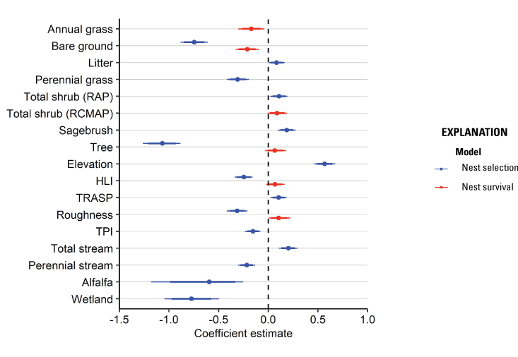
Habitat coefficient plots from models of greater sage-grouse (Centrocercus urophasianus) habitat selection and survival during the nesting life stage in the western Great Basin region, 2009–21. Models were fit using a hierarchical modeling framework subject to Bayesian lasso regularization and variable selection, with medians of posterior distributions represented by dots, thick lines representing one standard deviation, and thin lines representing the upper (97.5th) and lower (2.5th) percentiles of the distribution. The dashed vertical line occurs at zero and represents no effect. Abbreviations: RAP, Rangeland Analysis Platform; RCMAP, Rangeland Condition Monitoring Assessment and Projection; HLI, heat load index; TRASP, transformed aspect; TPI, topographic position index.
Habitat effects on nest survival were positive for total shrub cover, tree cover, HLI, and topographic roughness and were negative for annual grass cover and bare ground (table 2; fig. 2). All six habitat effects were interpreted as at least moderately informative (pd>0.9; table 2). In addition, there was little evidence for an effect of hen age on nest survival. Throughout the study area, cumulative 38-day nest survival was estimated to be 0.25 (95-percent credible intervals [CRI]=0.20–0.30). Predicted survival estimated from our final model of nest survival was consistent when compared with testing data (Bayesian P-value=0.59) and training data (Bayesian P-value=0.60) encounter histories, evidence that our model had good model fit and strong out-of-sample predictive capabilities.
Table 2.
Habitat coefficient summaries from models of greater sage-grouse (Centrocercus urophasianus) survival during the nesting and brood-rearing life stages in the western Great Basin region, 2009–21.[Logistic exposure models were fit using a Bayesian framework, and estimates reported include means and percentiles from posterior distributions, as well as the probability of direction (pd) statistic, indicating the proportion of the distribution falling on the same side of 0 as the median estimate. Abbreviations: NA, not applicable; m, meters; RCMAP, Rangeland Condition Monitoring Assessment and Projection; HLI, heat load index; TRASP, transformed aspect; TPI, topographic position index]
Brood Selection and Survival
We monitored 480 broods from 437 individual hens across all years and study sites collecting a total of 1,155 locations during the early brood-rearing period and 1,469 locations during the late brood-rearing period. The 95th percentile of distances between an individual’s brood location and its nest varied by study site with a median of 4,945 m during the early brood-rearing period (range: 1,123–11,758 m) and 11,631 m during the late brood-rearing period (range: 2,394–54,036 m). From variable selection analysis (for full results, see appendix 4), the most effective landscape predictor variables from correlated groups for the early brood habitat selection model component were bare ground (r=75 m), total shrub cover (RAP; r=75 m), tree cover (r=167 m), elevation (r=167 m), HLI (r=75 m), topographic roughness (r=75 m), TPI (r=1,451 m), total stream density (r=370 m), proximity to alfalfa (α=1,451), and proximity to wetland (α=0.24). For the late brood habitat selection component, the most effective predictor variables were annual grass cover (r=439 m), bare ground (r=75 m), litter cover (r=1451 m), perennial grass cover (r=75 m), total shrub cover (RCMAP; r=75 m), tree cover (r=439 m), elevation (r=260 m), HLI (r=370 m), topographic roughness (r=260 m), TPI (r=1,451 m), proximity to stream (α=1,451), proximity to alfalfa (α=1,451), whether or not an area was burned, and an interaction between annual grass and whether or not an area was burned. For brood survival models, during the early brood component the most effective predictors from variable selection were bare ground (r=439 m), litter cover (r=1,451 m), non-sagebrush shrub cover (r=1,451 m), tree cover (r=370 m), TRASP (r=1,451 m), topographic roughness (r=167 m), total stream density (r=167 m), proximity to alfalfa (α=1,451), and whether or not an area was burned. During the late brood component, the most effective survival predictors were annual grass cover (r=75 m), bare ground (r=1,451 m), TPI (r=75 m), total stream density (r=1,451 m), and proximity to perennial streams (α=1,451 m).
Broods demonstrated apparent selection of greater values for total shrub cover, elevation, TPI, and areas closer to alfalfa, while demonstrating apparent avoidance of greater values of bare ground, tree cover, HLI, and topographic roughness, during the early and late periods (table 1; fig. 3). Early broods demonstrated apparent avoidance of areas with higher total stream densities and closer proximities to wetlands, whereas late broods demonstrated apparent selection of areas closer to streams (table 1; fig. 3). Late broods also demonstrated apparent selection of annual grass, litter cover, perennial grass cover, and burned areas but demonstrated decreased selection for annual grass within burned areas. All habitat effects for the early and late brood-rearing periods were interpreted as moderately or strongly informative (table 1). Selection models had adequate out-of-sample predictive capabilities for the early (Spearman’s rank ρ=0.90; R2=0.73; βpredict=0.90) and late (Spearman’s rank ρ=0.95; R2=0.82; βpredict=0.68) brood-rearing periods.
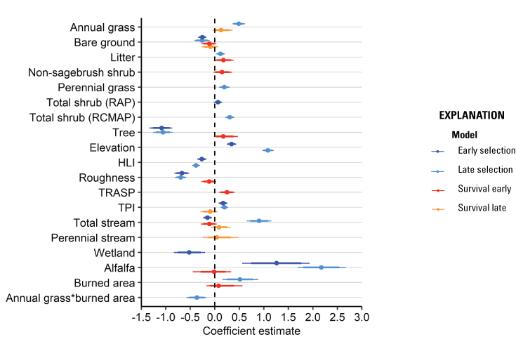
Habitat coefficient plots from models of greater sage-grouse (Centrocercus urophasianus) habitat selection and survival during the early brood-rearing (darker shades) and late brood-rearing (lighter shades) life stages in the western Great Basin region, 2009–21. Models were fit using a hierarchical modeling framework subject to Bayesian lasso regularization and variable selection, with medians of posterior distributions represented by dots, thick lines representing one standard deviation, and thin lines representing the upper (97.5th) and lower (2.5th) percentiles of the distribution. The dashed vertical line occurs at zero and represents no effect.
Habitat effects on brood survival were negative for bare ground for early and late periods. Early broods also demonstrated positive responses to litter cover, non-sagebrush shrub cover, tree cover, TRASP, and burned areas while demonstrating negative responses to topographic roughness, proximity to alfalfa, and total stream density (table 2; fig. 3). Late brood survival was lower with greater values of TPI and higher with more annual grass cover, greater total stream densities, and closer to perennial streams. Of the nine habitat effects estimated for early brood survival, seven were interpreted as moderately or strongly informative, with burned area indicating weaker evidence (table 2). For late brood survival, effects of annual grass cover, bare ground, and TPI were interpreted as moderately informative, with the remaining two habitat effects showing weaker evidence of effects (table 2). In addition, there was not moderate or strong evidence of an effect of hen age on brood survival, but there was evidence for a positive effect of brood age on survival (table 2). The estimated daily survival rate for broods was 0.985 (95-percent CRI=0.980–0.990). Predicted survival estimated from our final model of brood survival was consistent when compared with testing data (Bayesian P-value=0.64) and training data (Bayesian P-value=0.58) encounter histories, evidence that our model had good model fit and strong out-of-sample predictive capabilities.
Spring Selection
We monitored 2,171 individuals during the spring across years and study sites, collecting a total of 22,735 locations. The median 99-percent kernel UD for all birds at a study site was 1,431 square kilometers (km2; range: 720–3,743 km2). From variable selection analysis (for full results, see appendix 4), the most effective landscape predictor variables from correlated groups for the spring habitat selection model component were annual grass cover (r=75 m), bare ground (r=75 m), litter cover (r=439 m), perennial grass cover (r=1,451 m), total shrub cover (RAP; r=439 m), sagebrush cover (r=1,451 m), tree cover (r=439 m), elevation (r=167 m), HLI (r=439 m), TRASP (r=75 m), topographic roughness (r=167 m), TPI (r=439 m), total stream density (r=1,451 m), perennial stream density (r=1,451 m), log-transformed distance to alfalfa, and proximity to wetland (α=0.22). In the spring, sage-grouse demonstrated apparent selection for greater values of litter cover, sagebrush cover, elevation, TPI, total stream densities, and closer to alfalfa, while demonstrating apparent avoidance of areas with greater values for annual grass cover, bare ground, perennial grass cover, total shrub cover, tree cover, HLI, TRASP, topographic roughness, perennial stream densities, and closer to wetland (table 1; fig. 4). All 16 habitat effects were interpreted as strongly informative (table 1). The spring selection model had strong out-of-sample predictive capabilities (Spearman’s rank ρ=0.99; R2=0.94; βpredict=0.91).

Figure 4. Habitat coefficient plots from models of greater sage-grouse (Centrocercus urophasianus) habitat selection during the spring, summer, and winter in the western Great Basin region, 2009–21. Models were fit using a hierarchical modeling framework subject to Bayesian lasso regularization and variable selection, with medians of posterior distributions represented by dots, thick lines representing one standard deviation, and thin lines representing the upper (97.5th) and lower (2.5th) percentiles of the distribution. The dashed vertical line occurs at zero and represents no effect. Note that negative alfalfa effect for spring and summer selection are log(distance), which suggests selection.
Summer Selection
We monitored 1,778 individuals during the summer across years and study sites, collecting a total of 5,919 locations. The median 99-percent-kernel UD for all birds at a study site was 1,362 km2 (range: 493–3,141 km2). From variable selection analysis (for full results, see appendix 4), the most effective landscape predictors from correlated groups for the summer habitat selection model component were bare ground (r=1,451 m), litter cover (r=75 m), perennial grass cover (r=1,451 m), total shrub cover (RAP; r=1,451 m), total shrub cover (RCMAP; 75 m), tree cover (r=1,451 m), elevation (r=167 m), HLI (r=1,451 m), TRASP (r=1,451 m), topographic roughness (r=167 m), TPI (r=439 m), proximity to stream (α=540), proximity to perennial stream (α=1,451), log-transformed distance to alfalfa, proximity to wetland (α=0.18), and whether or not an area was burned. In the summer, sage-grouse demonstrated apparent selection of areas with greater values of total shrub cover within 75 m, elevation, TRASP, TPI, closer to total and perennial streams, and closer to alfalfa (table 1; fig. 4). Sage-grouse demonstrated apparent avoidance of areas with greater values of bare ground, litter cover, perennial grass cover, total shrub cover within 1,451 m, tree cover, HLI, topographic roughness, closer to wetlands, and burned areas (table 1; fig. 4). All 16 habitat effects were interpreted as strongly informative (table 1). The summer selection model had strong out-of-sample predictive capabilities (Spearman’s rank ρ=1.00; R2=0.92; βpredict=0.86).
Winter Selection
We monitored 264 individuals during winter across years and study sites, collecting a total of 5,508 locations. The median 99-percent kernel UD for all birds at a study site was 2,058 km2 (range: 946–4,110 km2). From variable selection analysis (for full results, see appendix 4), the most effective landscape predictor variables from correlated groups for the winter habitat selection model component were annual grass cover (r=370 m), bare ground (r=1,451 m), litter cover (r=439 m), total shrub cover (RCMAP; r=1,451 m), tree cover (r=1,451 m), elevation (r=75 m), HLI (r=1,451 m), TRASP (r=1,451 m), topographic roughness (r=439 m), TPI (r=439 m), proximity to stream (α=660), perennial stream density (r=439 m), proximity to alfalfa (α=1,451), and proximity to wetland (α=0.21). Wintering sage-grouse demonstrated apparent selection of areas with greater values for annual grass cover, litter cover, total shrub cover, elevation, TRASP, TPI, and closer to streams and alfalfa, while demonstrating apparent avoidance of areas with greater values for bare ground, tree cover, HLI, topographic roughness, perennial stream densities, and closer to wetland (table 1; fig. 4). Of the 14 habitat effects included in the final model, all were interpreted as strongly informative (table 1). The winter selection model had strong out-of-sample predictive capabilities (Spearman’s rank ρ=0.99; R2=0.97; βpredict=0.92).
Movement Model
We monitored 18 GPS-marked individuals to inform the resistance surface that was used to quantify connectivity between nesting and brood-rearing habitat. Based on an integrated step-selection model, females moving from nesting to brood-rearing habitat demonstrated apparent selection for greater total shrub cover, litter cover, higher densities of streams, areas closer to wetlands, higher elevations, and greater values of TPI (table 3). In contrast, females demonstrated apparent avoidance of higher tree cover, more bare ground, greater terrain roughness, and greater values of HLI (table 3).
Table 3.
Habitat coefficient summaries from a movement model of greater sage-grouse (Centrocercus urophasianus) transitioning from nesting to brood-rearing habitat in the western Great Basin region, 2009–21.[Logistic exposure models were fit using a Bayesian framework, and estimates reported include means and percentiles from posterior distributions, as well as the probability of direction (pd) statistic, indicating the proportion of the distribution falling on the same side of 0 as the median estimate. Abbreviations: HLI, heat load index; TPI, topographic position index]
Results: Habitat Mapping
Maps demonstrating seasonal sage-grouse selection patterns indicated that habitat potential (estimated from habitat selection models) was similar during the spring (fig. 5) and summer (fig. 6) but more widespread in the winter (fig. 7) when considering the overall area falling into the moderate or high categories. For reproductive life stages, habitat potential based on habitat selection models was more widespread across the study area during the nesting (fig. 8) and early brood-rearing periods (fig. 9) compared to the late brood-rearing period (fig. 10). Habitat suitability from survival models seemed possibly most limited during the nesting period (fig. 11) compared to the early brood-rearing (fig. 12) and late brood-rearing periods (fig. 13).
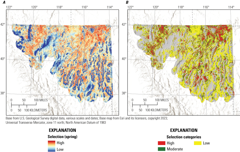
The A, habitat selection index and B, categorized habitat selection during the spring for greater sage-grouse (Centrocercus urophasianus) in the western Great Basin region, 2009–21. Predictions were developed from coefficients of habitat selection models fit within a hierarchical modeling framework subject to Bayesian lasso regularization and variable selection contrasting known locations from telemetry data with available locations in the western Great Basin region, 2009–21. Habitat classes were delineated based on percentiles of resource selection function values associated with known used locations of sage-grouse.
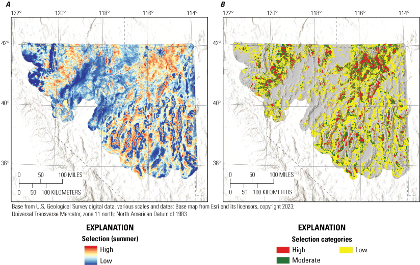
The A, habitat selection index and B, categorized habitat selection during the summer for greater sage-grouse (Centrocercus urophasianus) in the western Great Basin region, 2009–21. Predictions were developed from coefficients of habitat selection models fit within a hierarchical modeling framework subject to Bayesian lasso regularization and variable selection contrasting known locations from telemetry data with available locations in the western Great Basin region, 2009–21. Habitat classes were delineated based on percentiles of resource selection function values associated with known used locations of sage-grouse.
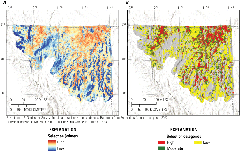
The A, habitat selection index and B, categorized habitat selection during the winter for greater sage-grouse (Centrocercus urophasianus) in the western Great Basin region, 2009–21. Predictions were developed from coefficients of habitat selection models fit within a hierarchical modeling framework subject to Bayesian lasso regularization and variable selection contrasting known locations from telemetry data with available locations in the western Great Basin region, 2009–21. Habitat classes were delineated based on percentiles of resource selection function values associated with known used locations of sage-grouse.
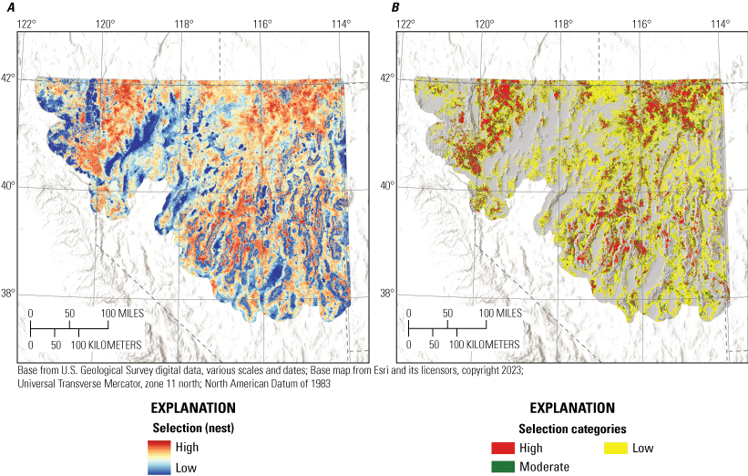
The A, habitat selection index and B, categorized habitat selection during the nesting period for greater sage-grouse (Centrocercus urophasianus) in the western Great Basin region, 2009–21. Predictions were developed from coefficients of habitat selection models fit within a hierarchical modeling framework subject to Bayesian lasso regularization and variable selection contrasting known locations from telemetry data with available locations in the western Great Basin region, 2009–21. Habitat classes were delineated based on percentiles of resource selection function values associated with known used locations of sage-grouse.
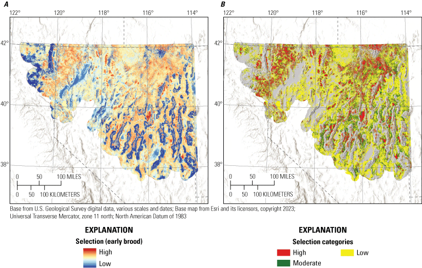
The A, habitat selection index and B, categorized habitat selection during the early brood-rearing period for greater sage-grouse (Centrocercus urophasianus) in the western Great Basin region, 2009–21. Predictions were developed from coefficients of habitat selection models fit within a hierarchical modeling framework subject to Bayesian lasso regularization and variable selection contrasting known locations from telemetry data with available locations in the western Great Basin region, 2009–21. Habitat classes were delineated based on percentiles of resource selection function values associated with known used locations of sage-grouse.
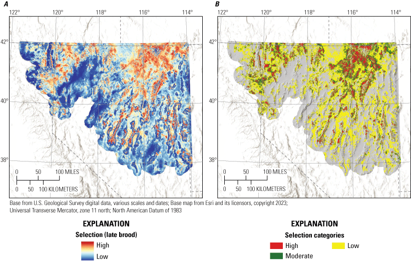
The A, habitat selection index and B, categorized habitat selection during the late brood-rearing period for greater sage-grouse (Centrocercus urophasianus) in the western Great Basin region, 2009–21. Predictions were developed from coefficients of habitat selection models fit within a hierarchical modeling framework subject to Bayesian lasso regularization and variable selection contrasting known locations from telemetry data with available locations in the western Great Basin region, 2009–21. Habitat classes were delineated based on percentiles of resource selection function values associated with known used locations of sage-grouse.
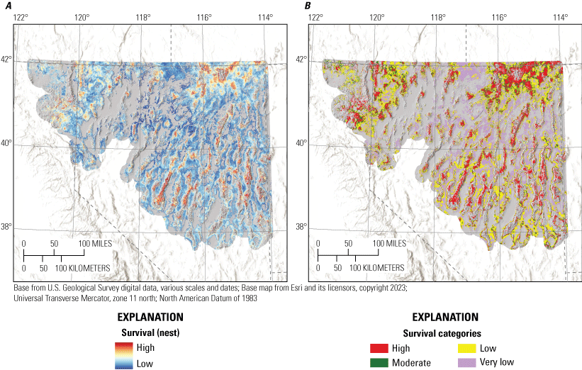
The A, overall survival and B, categorized survival during the nesting period for greater sage-grouse (Centrocercus urophasianus) in the western Great Basin region, 2009–21. Predictions were developed from coefficients of survival models fit within a hierarchical modeling framework subject to Bayesian lasso regularization and variable selection using encounter histories from marked birds in the western Great Basin region, 2009–21. Survival classes were delineated based on percentiles of cumulative survival values associated with successful and failed locations of sage-grouse.
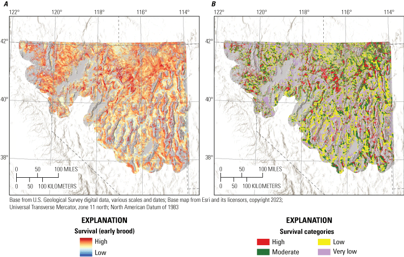
The A, overall survival and B, categorized survival during the early brood-rearing period for greater sage-grouse (Centrocercus urophasianus) in the western Great Basin region, 2009–21. Predictions were developed from coefficients of survival models fit within a hierarchical modeling framework subject to Bayesian lasso regularization and variable selection using encounter histories from marked birds in the western Great Basin region, 2009–21. Survival classes were delineated based on percentiles of cumulative survival values associated with successful and failed locations of sage-grouse.
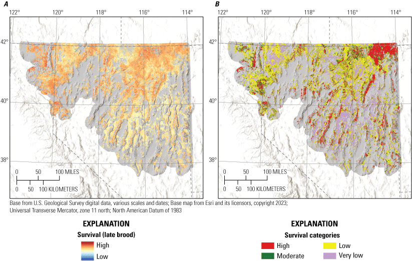
The A, overall survival and B, categorized survival during the late brood-rearing period for greater sage-grouse (Centrocercus urophasianus) in the western Great Basin region, 2009–21. Predictions were developed from coefficients of survival models fit within a hierarchical modeling framework subject to Bayesian lasso regularization and variable selection using encounter histories from marked birds in the western Great Basin region, 2009–21. Survival classes were delineated based on percentiles of cumulative survival values associated with successful and failed locations of sage-grouse.
Areas of high-use based on the ASUI (fig. 14) generally aligned with areas of high use based on the habitat selection models (figs. 5–10) and the combined metric of habitat suitability and occupancy (appendix 5). Priority habitat seemed to be concentrated in the northern parts of California and Nevada and more fragmented in the southern parts of the study area (fig. 15). A total of 1.5 percent of the study area was classified as priority+ (5,112 km2), 15.5 percent as priority (51,683 km2), 6.4 percent as general (21,359 km2), and 9.1 percent as other (30,410 km2) with the remainder classified as non-habitat. Including corridors that connect occupied nesting habitat to brood source habitat resulted in small increases in general habitat (0.18 percent), particularly in the southern part of the study area (fig. 16).
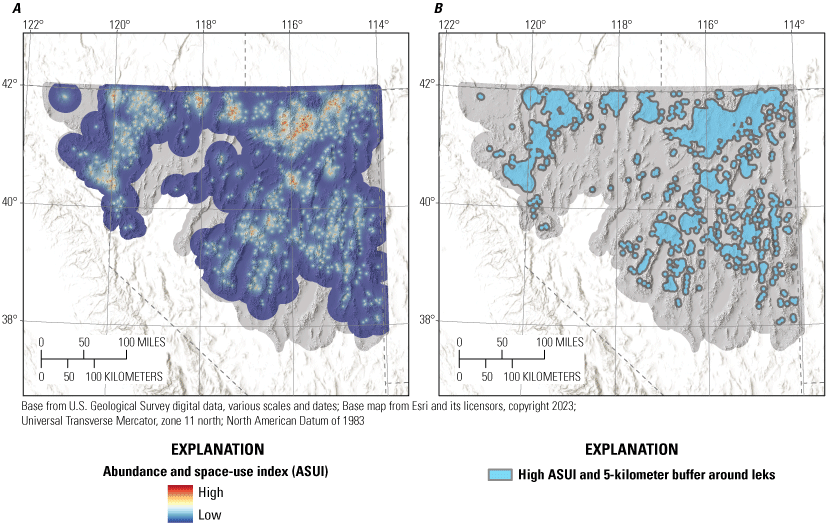
The A, continuous and B, categorized abundance and space use index (ASUI) for greater sage-grouse (Centrocercus urophasianus) in the western Great Basin region, 2013–21. Peak male sage-grouse abundances at leks were used as input into kernel density models to generate a surface denoting high use (greater than 85-percent isopleth).
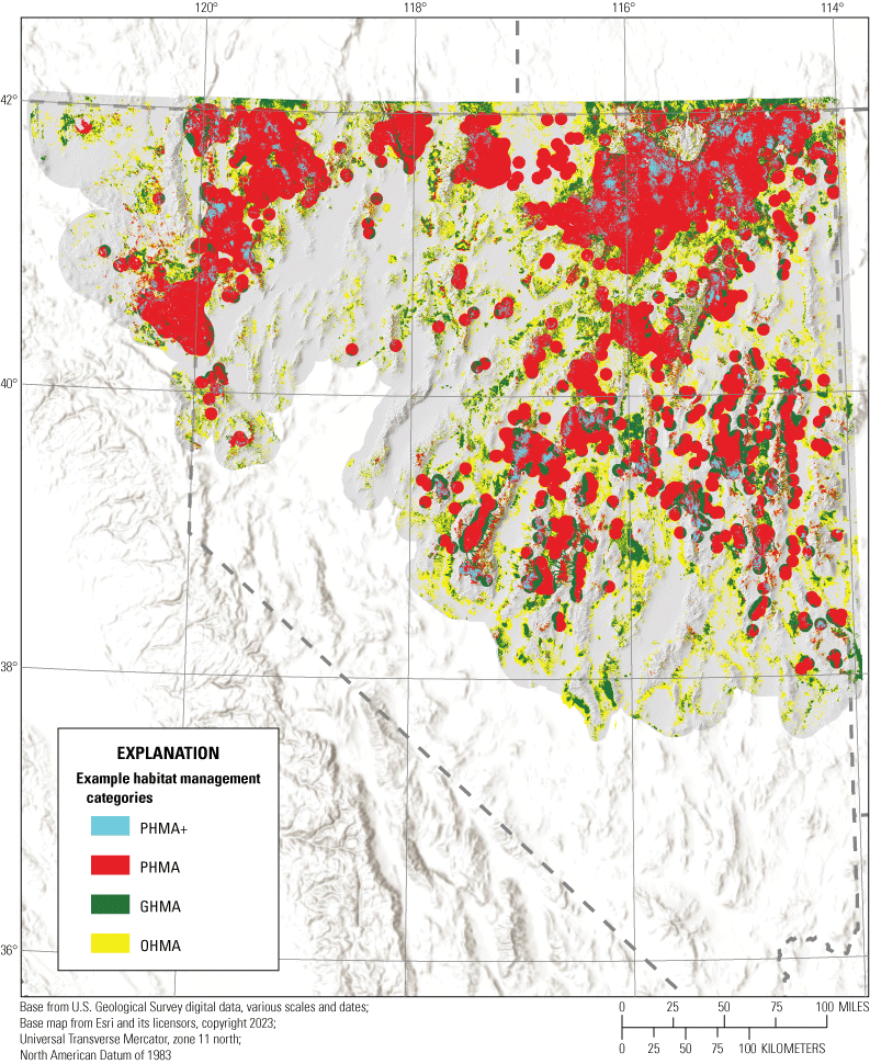
The example habitat management categories delineated for greater sage-grouse (Centrocercus urophasianus) in the western Great Basin region, 2009–21. The categorized selection maps and maps of source habitat describing areas of high selection and high survival for a specific life stage or season were combined with the abundance and space use index to delineate four management categories. Priority+ captures the best sage-grouse habitat with a high certainty of current occupancy. Priority habitat includes areas that support sage-grouse with high certainty of current occupancy plus the best source habitat with low potential for occupancy and lek locations. General habitat includes high-quality habitat that has a low potential for occupancy and potentially occupied areas in low-quality habitat. Other habitat captures areas used less frequently by sage-grouse where conditions may still be conducive for occupancy. Abbreviations: PHMA+, priority+ habitat management area; PHMA, priority habitat management area; GHMA, general habitat management area; OHMA, other habitat management area.
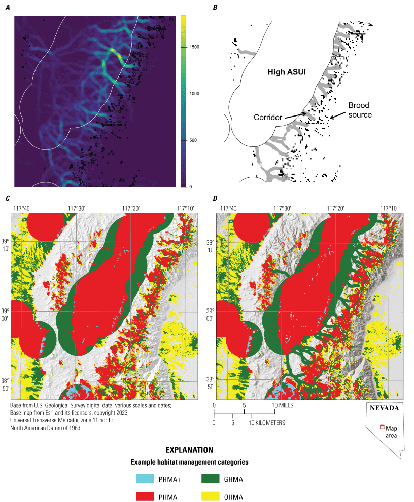
Examples of the corridors delineated for greater sage-grouse (Centrocercus urophasianus) in the western Great Basin region, 2009–21, connecting occupied nest habitat with brood source habitat, including the A, output of the least cost paths analysis; B, identified corridors in grey connecting an area of high abundance and space use index to brood source habitat in black; C, example habitat management categories before inclusion of the corridors; and D, example habitat management categories with the corridors included. The least-cost paths analysis identified areas that could serve as corridors between areas of high abundance and areas identified as source areas for broods, with the underlying resistance layer developed using movement data from Global Positioning System-tracked sage-grouse. Abbreviations: PHMA+, priority+ habitat management area; PHMA, priority habitat management area; GHMA, general habitat management area; OHMA, other habitat management area.
Interpretation and Synthesis
We investigated habitat responses of sage-grouse by evaluating habitat selection and survival patterns across distinct seasons and life stages to guide conservation and management decision-making. This comprehensive approach allowed us to highlight habitat features that were consistently important across the annual life cycle of sage-grouse but also identify features for which selection and survival responses differed, indicating potential maladaptive selection (Remeš, 2000; Pratt and Beck, 2021). Habitat selection can become maladaptive when individuals select areas that reduce their demographic performance, and this is becoming more pronounced in rapidly changing environments, such as sagebrush ecosystems within the Great Basin (Anthony and others, 2021; Brussee and others, 2022; Merkle and others, 2022). Resource selection analyses and subsequent habitat maps are regularly used to guide management actions, but focusing solely on selection patterns could result in management decisions that inadvertently promote ecological traps (Battin, 2004; Hale and Swearer, 2017). In contrast, evaluating selection and demographic performance, particularly across multiple life stages, as done here, can highlight both important source habitats that support high selection and high survival and thus have critical value for long-term conservation, and sink habitats that support high selection but low success and may represent key areas to target for restoration. In addition, our efforts integrating measures of selection and demographic performance with information on the distribution of current occupancy will likely better guide landscape-scale management decisions. The modeling and mapping efforts demonstrated in this work represent a comprehensive approach that combines and updates previous efforts (Coates and others, 2020a; O’Neil and others, 2020; Brussee and others, 2022) with all current datasets, new information on spring and summer habitat selection, an updated abundance and space use index, and additional analyses to represent pre-fire conditions and connectivity between important nesting and brood-rearing habitat. Overall, we delineated example habitat management categories that can be used to guide conservation and management actions, with 1.5 percent of the study area classified as priority+, 15.5 percent as priority, 6.4 percent as general, and 9.1 percent as other habitat. We discuss specific findings regarding the habitat responses of sage-grouse and their relevance to management in the next paragraphs.
Our findings revealed consistent patterns of sage-grouse habitat selection, and generally survival responses, for some key environmental characteristics such as shrub, sagebrush, higher relative elevations, and tree cover. However, habitat responses were more nuanced with respect to topographic indices, and moisture and agriculture variables (for example, stream densities and proximity to wetlands or meadows and alfalfa fields). Sage-grouse had strong selection responses to total shrub cover during summer and brood-rearing life stages, whereas sagebrush cover was a better predictor during spring and nesting. Other important vegetation components were tree cover and bare ground, where larger values typically corresponded to avoidance by sage-grouse or reduced survival across multiple life stages. Trees and expanding conifer cover have largely been associated with negative effects to sage-grouse in most places where it has been studied (Coates and others, 2017; Prochazka and others, 2017; Sandford and others, 2017; Severson and others, 2017; Olsen and others, 2021), mainly because tree expansion leads to loss of sagebrush and herbaceous cover, and trees provide nest and perch substrate for certain predators. Although we observed the expected negative response in association with habitat selection across all life stages, we observed weak evidence of increased survival response to tree cover during nesting and early brood-rearing. Because of strong avoidance, a positive survival response suggests that relatively small amounts of tree cover are occasionally used during these life stages, and these trees may be highly associated with upland riparian areas, which are important to survival. More complex models that fit interactions between trees and riparian areas would be beneficial. Importantly, conifers occur at higher elevations where other habitat characteristics collectively tend to support greater survival (Billings, 1951; Miller and others, 2008; Gibson and others, 2017).
Although responses to vegetation variables were generally consistent across life stages, responses to topographic, moisture, and agriculture variables were more varied. Sage-grouse demonstrated strong selection responses for higher elevations, which is consistent with previous studies (Freese and others, 2016; Blomberg and others, 2017; Gibson and others, 2017), although effects on survival were largely neutral. Effects of other topographic variables varied by life stage. Selection based on topographic position index was negative during nesting but positive during spring, summer, winter, and brood-rearing, which suggests selection for higher ridges later during the reproductive season and is consistent with previous studies (Freese and others, 2016; Gibson and others, 2017). Greater topographic roughness was avoided during all seasons and life stages despite a positive effect on nest survival, a pattern which has been observed previously (Coates and others, 2019; O’Neil and others, 2020). Sage-grouse also avoided higher heat loads across seasons and life stages, although we observed weak evidence of a positive effect on nest survival. Similarly, selection and survival responses for moisture variables including streams and wetlands differed across life stages. Sage-grouse avoided perennial streams during the spring, winter, and nesting and all streams during early brood-rearing but demonstrated strong selection for all streams during spring, summer, winter, nesting, and late brood-rearing. Survival responses also differed, with a negative effect of streams during early brood-rearing but a positive effect during late brood-rearing. Wetlands and wet meadows were more consistently avoided during spring, nesting, early brood-rearing, summer, and winter. Overall, seasonal differences suggest a shift in habitat use from early to late brood-rearing when access to moisture becomes increasingly important but that wet riparian areas are evidently risky during other life stages, which is consistent with previous research (Casazza and others, 2011; Dzialak and others, 2015; Donnelly and others, 2016; Coates and others, 2020a). Responses to alfalfa fields were also more variable across seasons and life stages. Sage-grouse demonstrated strong avoidance of alfalfa fields during nesting. In contrast, sage-grouse demonstrated selection responses for alfalfa fields during the spring, summer, and early and late brood-rearing, despite experiencing lower survival during the early brood-rearing period near alfalfa fields. Cropland conversion removes sagebrush ecosystems and can threaten sage-grouse persistence at large spatial scales (Smith and others, 2016) by providing anthropogenic subsidies for predators, such as ravens (Coates and others, 2016a, 2020b), but consistent with our findings, sage-grouse can have inconsistent and possibly maladaptive responses to irrigated croplands at small scales (Pratt and Beck, 2021).
By evaluating habitat selection and survival responses across multiple life stages, we were able to highlight situations in which selection may not be adaptive or where selection in one life stage may affect survival in a different stage. For example, sage-grouse had strong selection responses for perennial and annual grass during late brood-rearing and moderate selection for annual grass during winter, but there was no clear evidence of a survival response to perennial grass. However, during the late brood-rearing period, selection for annual grass was reduced in burned areas, although reductions were not sufficient to result in strong avoidance. Despite finding evidence of a positive effect of annual grass cover on late brood survival, previous studies indicate that brood survival in the Great Basin decreased with greater annual grass cover but only in the presence of wildfire (Brussee and others, 2022). Wildfire can have negative effects across multiple life stages (Foster and others, 2019; O’Neil and others, 2020; Anthony and others, 2021; Dudley and others, 2021), largely a result of a positive feedback loop between wildfire and invasive annual grasses (Germino and others, 2016; Condon and Pyke, 2018). Sage-grouse also selected for greater litter cover during spring, nesting, late brood-rearing, and winter, despite no observed effects on nest survival. Given the positive effects on survival during early brood-rearing, selection during nesting likely represents a tradeoff where selection patterns that increase one aspect of fitness have a negative or neutral effect on another component (Battin, 2004; Stamps and others, 2005). Such tradeoffs have been previously identified for sage-grouse, such as when birds may select specific components of nesting habitat because it increases chick survival instead of nest survival (Gibson and others, 2016). Tradeoffs highlight the importance of evaluating selection and survival across multiple life stages, because focusing on a single life stage can miss important constraints where habitat use can affect multiple components of fitness (Chalfoun and Martin, 2007; Gibson and others, 2016).
Our analysis was not without caveats and considerations. We intentionally did not include anthropogenic factors in this analysis because our objective was to predict sage-grouse habitat as a function of natural environmental characteristics across the landscape. One potential exception to this was the inclusion of agricultural areas. We included agricultural areas and changes in land cover associated with wildfire because these areas represent land cover that are often used by sage-grouse at relatively broader scales and are thought to affect sage-grouse populations positively and negatively. We recognize that anthropogenic features, such as roads and transmission lines, could also be important drivers of sage-grouse selection and demographic responses, but these types of point sources do not represent major land cover changes. We also recognize the importance of incorporating anthropogenic features into analyses that use modeled outputs presented here when assessing specific areas for conservation and management decisions. Another important limitation to our study was brood survival was modeled as binary data type, indicating presence or absence instead of chick survival. Modeling brood survival inevitably results in a loss of information and limits the scope of our results regarding the brood-rearing life stage. Information on chick survival could improve resolution regarding features affecting bird mortality but is often difficult to reliably collect. Analyses of brood survival can provide information on factors affecting overall brood success, but future analyses could consider chick survival when such data are available.
Although resource selection maps are often used to guide or prioritize management actions, we included an additional layer of information by creating maps of selection and survival. The selection maps (figs. 5–10) provide important information on areas used by sage-grouse but when used without information on survival, can lead to decisions that inadvertently promote ecological traps by prioritizing areas with high selection but low survival. In contrast, survival maps (figs. 11–13) focus on population performance but may not increase local distribution if not used in conjunction with information on areas used by birds. Importantly, our approach evaluated habitat selection and survival responses across multiple seasons and life stages, thus allowing the identification of key habitats that may disproportionately affect populations during critical periods but may go undetected when considering effects throughout an annual period.
In addition to identifying habitats important for individual seasons or life stages, we also accounted for movement between these areas by delineating corridors between key nesting and brood-rearing habitats. Although we did not have sufficient data to empirically identify corridors based on sage-grouse movements across the study area, we used fine resolution movement data from GPS-marked individuals to develop a resistance surface representing movement potential across the landscape, which is the preferred data source for connectivity analyses (Zeller and others, 2012). Although these areas may not constitute high-quality habitat by themselves, they represent important movement corridors between fragmented patches that are used at different life stages, and it is important to recognize their conservation value. Importantly, the LCP analysis to identify corridors could benefit from additional data from GPS-marked sage-grouse, particularly in areas where potential corridors were identified. Ideally, the delineation of corridors would be determined empirically by observing the movements of sage-grouse. However, it is unrealistic to expect available data to cover the extent examined here. In the absence of range-wide data, methods like LCP analysis can be used to make predictions as to the location of corridors. The LCP methods are not without criticisms, however. Animal movement may follow a non-optimal path instead of the route identified by the LCP algorithm (Fahrig, 2007). In addition, the fact that the LCP algorithm only selects a single, 1-pixel wide path means that other high-quality paths may be ignored (Sawyer and others, 2011). Although this issue is partially addressed in our methodology by selecting 10,000 random points and finding paths to every source cell within 15.3 km, this does not completely solve the issue because the paths still tend to coalesce to a few, low-cost areas. Additionally, the use of a moving-window to widen the paths, though useful for visualization and analysis purposes, does not remedy the fact that only single-pixel-width paths were used in generating the original LCPs. Another weakness is the arbitrary selection of the 95th percentile for determining which areas are designated as corridors. While this cutoff serves to limit the identified corridors to those with the most LCPs, a better thresholding method would take empirical movement into account to determine the threshold used to create the binary raster.
Finally, we incorporated an improved abundance and space use index, which when combined with the habitat selection and survival layers, allowed us to delineate example habitat management categories. Our updated abundance and space use index was based on abundance estimates from recent hierarchical modeling done across the region (Coates and others, 2022), and incorporated estimation for leks that lacked enough information to be included in the hierarchical modeling. As a result, the updated abundance and space use index provided a better representation of all leks across the study area and thus an improved depiction of currently occupied habitat in Nevada and northeastern California. By considering the distribution of current occupancy, our approach to identifying habitat suitability allows priority areas to be highlighted for habitat preservation. For example, source habitat, with high selection and high survival, has key value for long-term conservation (O’Neil and others, 2020; Brussee and others, 2022; Saher and others, 2022) particularly when in currently occupied areas, which is designated as priority+ in our example habitat management categories and represented a total of 1.5 percent of our study area. Our approach can also identify areas where anthropogenic development can occur with minimal effect and highlight areas where management and restoration activities are likely to have the greatest benefit, such as in occupied areas with lower predicted habitat quality. Overall, by evaluating selection and survival responses across multiple life stages, our maps provide detailed information that can allow for a more flexible and targeted management approach. The power of this approach lies within the combination of multiple map outputs that can be directed toward local level efforts to help inform specific management decisions, with full recognition that on-the-ground field data and other sources of information and expertise should be used in conjunction with inferences from these models.
References Cited
Aarts, G., Fieberg, J., and Matthiopoulos, J., 2012, Comparative interpretation of count, presence-absence and point methods for species distribution models: Methods in Ecology and Evolution, v. 3, no. 1, p. 177–187. [Available at https://doi.org/10.1111/j.2041-210X.2011.00141.x.]
Adriaensen, F., Chardon, J.P., De Blust, G., Swinnen, E., Villalba, S., Gulinck, H., and Matthysen, E., 2003, The application of ‘least-cost’ modelling as a functional landscape model: Landscape and Urban Planning, v. 64, no. 4, p. 233–247. [Available at https://doi.org/10.1016/S0169-2046(02)00242-6.]
Aldridge, C.L., Nielsen, S.E., Beyer, H.L., Boyce, M.S., Connelly, J.W., Knick, S.T., and Schroeder, M.A., 2008, Range‐wide patterns of greater sage‐grouse persistence: Diversity and Distributions, v. 14, no. 6, p. 983–994. [Available at https://doi.org/10.1111/j.1472-4642.2008.00502.x.]
Allred, B.W., Bestelmeyer, B.T., Boyd, C.S., Brown, C., Davies, K.W., Duniway, M.C., Ellsworth, L.M., Erickson, T.A., Fuhlendorf, S.D., Griffiths, T.V., Jansen, V., Jones, M.O., Karl, J., Knight, A., Maestas, J.D., Maynard, J.J., McCord, S.E., Naugle, D.E., Starns, H.D., Twidwell, D., and Uden, D.R., 2021, Improving Landsat predictions of rangeland fractional cover with multitask learning and uncertainty: Methods in Ecology and Evolution, v. 12, no. 5, p. 841–849. [Available at https://doi.org/10.1111/2041-210X.13564.]
Andreadis, K.M., and Lettenmaier, D.P., 2006, Trends in 20th century drought over the continental United States: Geophysical Research Letters, v. 33, no. 10, p. 1–4. [Available at https://doi.org/10.1029/2006GL025711.]
Anthony, C.R., Foster, L.J., Hagen, C.A., and Dugger, K.M., 2021, Acute and lagged fitness consequences for a sagebrush obligate in a post mega‐wildfire landscape: Ecology and Evolution, v. 12, no. 1, 12 p. [Available at https://doi.org/10.1002/ece3.8488.]
Avgar, T., Potts, J.R., Lewis, M.A., and Boyce, M.S., 2016, Integrated step selection analysis—Bridging the gap between resource selection and animal movement: Methods in Ecology and Evolution, v. 7, no. 5, p. 619–630. [Available at https://doi.org/10.1111/2041-210X.12528.]
Battin, J., 2004, When good animals love bad habitats—Ecological traps and the conservation of animal populations: Conservation Biology, v. 18, no. 6, p. 1482–1491. [Available at https://doi.org/10.1111/j.1523-1739.2004.00417.x.]
Blomberg, E.J., Gibson, D., Atamian, M.T., and Sedinger, J.S., 2017, Variable drivers of primary versus secondary nesting—Density‐dependence and drought effects on greater sage‐grouse: Journal of Avian Biology, v. 48, no. 6, p. 827–836. [Available at https://doi.org/10.1111/jav.00988.]
Blomberg, E.J., Sedinger, J.S., Nonne, D.V., and Atamian, M.T., 2013, Seasonal reproductive costs contribute to reduced survival of female greater sage-grouse: Journal of Avian Biology, v. 44, no. 2, p. 149–158. [Available at https://doi.org/10.1111/j.1600-048X.2012.00013.x.]
Boyd, C.S., Davies, K.W., and Collins, G.H., 2017, Impacts of feral horse use on herbaceous riparian vegetation within a sagebrush steppe ecosystem: Rangeland Ecology & Management, v. 70, no. 4, p. 411–417. [Available at https://doi.org/10.1016/j.rama.2017.02.001.]
Brussee, B.E., Coates, P.S., O’Neil, S.T., Casazza, M.L., Espinosa, S.P., Boone, J.D., Ammon, E.M., Gardner, S.C., and Delehanty, D.J., 2022, Invasion of annual grasses following wildfire corresponds to maladaptive habitat selection by a sagebrush ecosystem indicator species: Global Ecology and Conservation, v. 37, 19 p. [Available at https://doi.org/10.1016/j.gecco.2022.e02147.]
Brussee, B.E., Coates, P.S., O’Neil, S.T., Ricca, M.A., Dudko, J.E., Espinosa, S.P., Gardner, S.C., Casazza, M.L., and Delehanty, D.J., 2023, Influence of fine-scale habitat characteristics on sage-grouse nest site selection and nest survival varies by mesic and xeric site conditions: Ornithological Applications, v. 125, no. 1, 15 p., accessed July 14, 2022, at https://doi.org/10.1093/ornithapp/duac052.
Bureau of Land Management, 2015, Notice of availability of the record of decision and approved resource management plan amendments for the Great Basin region greater sage-grouse sub-regions of Idaho and southwestern Montana, Nevada and northeastern California, Oregon, and Utah: Federal Register, v. 80, no. 185, p. 57633–57636, accessed June 20, 2023, at https://www.govinfo.gov/content/pkg/FR-2015-09-24/pdf/2015-24213.pdf.
Bureau of Land Management, 2021, Notice of intent to amend land use plans regarding greater sage-grouse conservation and prepare associated environmental impact statements: Federal Register, v. 86, no. 222, p. 66331–66333, accessed June 20, 2023, at https://www.govinfo.gov/content/pkg/FR-2021-11-22/pdf/2021-25393.pdf.
Catlin, D.H., Fraser, J.D., and Felio, J.H., 2015, Demographic responses of Piping Plovers to habitat creation on the Missouri River: Wildlife Monographs, v. 192, no. 1, p. 1–42. [Available at https://doi.org/10.1002/wmon.1016.]
Chalfoun, A.D., and Martin, T.E., 2007, Assessments of habitat preferences and quality depend on spatial scale and metrics of fitness: Journal of Applied Ecology, v. 44, no. 5, p. 983–992. [Available at https://doi.org/10.1111/j.1365-2664.2007.01352.x.]
Coates, P.S., Brussee, B.E., Howe, K.B., Gustafson, K.B., Casazza, M.L., and Delehanty, D.J., 2016a, Landscape characteristics and livestock presence influence common ravens—Relevance to greater sage-grouse conservation: Ecosphere, v. 7, no. 2, 20 p. [Available at https://doi.org/10.1002/ecs2.1203.]
Coates, P.S., Brussee, B.E., Ricca, M.A., Severson, J.P., Casazza, M.L., Gustafson, K.B., Espinosa, S.P., Gardner, S.C., and Delehanty, D.J., 2020a, Spatially explicit models of seasonal habitat for greater sage-grouse at broad spatial scales—Informing areas for management in Nevada and northeastern California: Ecology and Evolution, v. 10, no. 1, p. 104–118. [Available at https://doi.org/10.1002/ece3.5842.]
Coates, P.S., Casazza, M.L., Blomberg, E.J., Gardner, S.C., Espinosa, S.P., Yee, J.L., Wiechman, L., and Halstead, B.J., 2013, Evaluating greater sage-grouse seasonal space use relative to leks—Implications for surface use designations in sagebrush ecosystems: The Journal of Wildlife Management, v. 77, no. 8, p. 1598–1609. [Available at https://doi.org/10.1002/jwmg.618.]
Coates, P.S., Casazza, M.L., Ricca, M.A., Brussee, B.E., Blomberg, E.J., Gustafson, K.B., Overton, C.T., Davis, D.M., Niell, L.E., Espinosa, S.P., Gardner, S.C., and Delehanty, D.J., 2016b, Integrating spatially explicit indices of abundance and habitat quality—An applied example for greater sage-grouse management: Journal of Applied Ecology, v. 53, no. 1, p. 83–95. [Available at https://doi.org/10.1111/1365-2664.12558.]
Coates, P.S., Milligan, M.C., O’Neil, S.T., Brussee, B.E., and Chenaille, M.P., 2024, Rasters representing Greater sage-grouse space use, habitat selection, and survival to inform habitat management: U.S. Geological Survey data release. [Available at https://doi.org/10.5066/P933VE6W.]
Coates, P.S., O’Neil, S.T., Brussee, B.E., Ricca, M.A., Jackson, P.J., Dinkins, J.B., Howe, K.B., Moser, A.M., Foster, L.J., and Delehanty, D.J., 2020b, Broad-scale impacts of an invasive native predator on a sensitive native prey species within the shifting avian community of the North American Great Basin: Biological Conservation, v. 243, 10 p. [Available at https://doi.org/10.1016/j.biocon.2020.108409.]
Coates, P.S., O’Neil, S.T., Muñoz, D.A., Dwight, I.A., and Tull, J.C., 2021a, Sage-grouse population dynamics are adversely affected by overabundant feral horses: The Journal of Wildlife Management, v. 85, no. 6, p. 1132–1149. [Available at https://doi.org/10.1002/jwmg.22089.]
Coates, P.S., Prochazka, B.G., Aldridge, C.L., O’Donnell, M.S., Edmunds, D.R., Monroe, A.P., Hanser, S.E., Wiechman, L.A., and Chenaille, M.P., 2022, Range-wide population trend analysis for greater sage-grouse (Centrocercus urophasianus)—Updated 1960–2021: U.S. Geological Survey Data Report 1165, 16 p., accessed September 16, 2023, at https://doi.org/10.3133/dr1165.
Coates, P.S., Prochazka, B.G., O’Donnell, M.S., Aldridge, C.L., Edmunds, D.R., Monroe, A.P., Ricca, M.A., Wann, G.T., Hanser, S.E., Wiechman, L.A., and Chenaille, M.P., 2021b, Range-wide greater sage-grouse hierarchical monitoring framework—Implications for defining population boundaries, trend estimation, and a targeted annual warning system: U.S. Geological Survey Open-File Report 2020–1154, 243 p., accessed September 23, 2022, at https://doi.org/10.3133/ofr20201154.
Coates, P.S., Ricca, M.A., Prochazka, B.G., Brooks, M.L., Doherty, K.E., Kroger, T., Blomberg, E.J., Hagen, C.A., and Casazza, M.L., 2016c, Wildfire, climate, and invasive grass interactions negatively impact an indicator species by reshaping sagebrush ecosystems: Proceedings of the National Academy of Sciences of the United States of America, v. 113, no. 45, p. 12745–12750. [Available at https://doi.org/10.1073/pnas.1606898113.]
Coates, P.S., Ricca, M.A., Prochazka, B.G., O’Neil, S.T., Severson, J.P., Mathews, S.R., Espinosa, S., Gardner, S., Lisius, S., and Delehanty, D.J., 2019, Population and habitat analyses for Greater Sage-Grouse (Centrocercus urophasianus) in the bi-state distinct population segment—2018 update: U.S. Geological Survey Open-File Report 2019–1149, 122 p., accessed January 27, 2021, at https://doi.org/10.3133/ofr20191149.
Coates, P.S., Prochazka, B.G., Ricca, M.A., Gustafson, K.B., Ziegler, P., and Casazza, M.L., 2017, Pinyon and juniper encroachment into sagebrush ecosystems impacts distribution and survival of greater sage-grouse: Rangeland Ecology & Management, v. 70, no. 1, p. 25–38. [Available at https://doi.org/10.1016/j.rama.2016.09.001.]
Condon, L.A., and Pyke, D.A., 2018, Fire and grazing influence site resistance to Bromus tectorum through their effects on shrub, bunchgrass and biocrust communities in the Great Basin (USA): Ecosystems (New York, N.Y.), v. 21, no. 7, p. 1416–1431. [Available at https://doi.org/10.1007/s10021-018-0230-8.]
Connelly, J.W., and Braun, C.E., 1997, Long-term changes in sage grouse Centrocercus urophasianus populations in western North America: Wildlife Biology, v. 3, nos. 3–4, p. 229–234. [Available at https://doi.org/10.2981/wlb.1997.028.]
Cutting, K.A., Rotella, J.J., Schroff, S.R., Frisina, M.R., Waxe, J.A., Nunlist, E., and Sowell, B.F., 2019, Maladaptive nest-site selection by a sagebrush dependent species in a grazing-modified landscape: Journal of Environmental Management, v. 236, p. 622–630. [Available at https://doi.org/10.1016/j.jenvman.2019.01.085.]
Davies, K.W., and Bates, J.D., 2017, Restoring big sagebrush after controlling encroaching western juniper with fire—Aspect and subspecies effects: Restoration Ecology, v. 25, no. 1, p. 33–41. [Available at https://doi.org/10.1111/rec.12375.]
De Reu, J., Bourgeois, J., Bats, M., Zwertvaegher, A., Gelorini, V., De Smedt, P., Chu, W., Antrop, M., De Maeyer, P., Finke, P., Van Meirvenne, M., Verniers, J., and Crombé, P., 2013, Application of the topographic position index to heterogeneous landscapes: Geomorphology, v. 186, p. 39–49. [Available at https://doi.org/10.1016/j.geomorph.2012.12.015.]
de Valpine, P., Paciorek, C.J., Turek, D., Michaud, N., Anderson-Bergman, C., Obermeyer, F., Wehrhahn Cortes, C., Rodriguez, A., Temple Lang, D., and Paganin, S., 2022, NIMBLE—MCMC, Particle Filtering, and Programmable Hierarchical Modeling: R Package Version 0.13.0, NIMBLE Development Team, accessed March 3, 2023, at https://doi.org/10.5281/zenodo.1211190.
de Valpine, P., Turek, D., Paciorek, C.J., Anderson-Bergman, C., Lang, D.T., and Bodik, R., 2017, Programming with models—Writing statistical algorithms for general model structures with NIMBLE: Journal of Computational and Graphical Statistics, v. 26, no. 2, p. 403–413. [Available at https://doi.org/10.1080/10618600.2016.1172487.]
Dewitz, J., and U.S. Geological Survey, 2021, National Land Cover Database (NLCD) 2019 Products: U.S. Geological Survey data release v. 2.0, accessed June 13, 2023, at https://www.mrlc.gov/data/nlcd-imperviousness-conus-all-years.
Dijkstra, E.W., Beauguitte, L., and Maisonobe, M., 1959, A note on two problems in connexion with graphs: Numerische Mathematik, v. 1, p. 269–271. [Available at https://doi.org/10.1007/BF01386390.]
Doherty, K.E., Evans, J.S., Coates, P.S., Juliusson, L.M., and Fedy, B.C., 2016, Importance of regional variation in conservation planning—A rangewide example of the Greater Sage-Grouse: Ecosphere, v. 7, no. 10, 27 p. [Available at https://doi.org/10.1002/ecs2.1462.]
Donnelly, J.P., Allred, B.W., Perret, D., Silverman, N.L., Tack, J.D., Dreitz, V.J., Maestas, J.D., and Naugle, D.E., 2018, Seasonal drought in North America’s sagebrush biome structures dynamic mesic resources for sage-grouse: Ecology and Evolution, v. 8, no. 24, p. 12492–12505. [Available at https://doi.org/10.1002/ece3.4614.]
Donnelly, J., Naugle, D., Hagen, C., and Maestas, J., 2016, Public lands and private waters—Scarce mesic resources structure land tenure and sage-grouse distributions: Ecosphere, v. 7, no. 1, 15 p. [Available at https://doi.org/10.1002/ecs2.1208.]
Dormann, C.F., Elith, J., Bacher, S., Buchmann, C., Carl, G., Carré, G., Marquéz, J.R.G., Gruber, B., Lafourcade, B., Leitão, P.J., Münkemüller, T., McClean, C., Osborne, P.E., Reineking, B., Schröder, B., Skidmore, A.K., Zurell, D., and Lautenbach, S., 2013, Collinearity—A review of methods to deal with it and a simulation study evaluating their performance: Ecography, v. 36, no. 1, p. 27–46. [Available at https://doi.org/10.1111/j.1600-0587.2012.07348.x.]
Dudko, J.E., Coates, P.S., and Delehanty, D.J., 2018, Movements of female Sage Grouse Centrocercus urophasianus during incubation recess: The Ibis, v. 161, no. 1, p. 222–229. [Available at https://doi.org/10.1111/ibi.12670.]
Dudley, I.F., Coates, P.S., Prochazka, B.G., O’Neil, S.T., Gardner, S., and Delehanty, D.J., 2021, Large-scale wildfire reduces population growth in a peripheral population of sage-grouse: Fire Ecology, v. 17, article 15, 13 p. [Available at https://doi.org/10.1186/s42408-021-00099-z.]
Dzialak, M.R., Olson, C.V., Webb, S.L., Harju, S.M., and Winstead, J.B., 2015, Incorporating within- and between-patch resource selection in identification of critical habitat for broodrearing greater sage-grouse: Ecological Processes, v. 4, article 5, 15 p. [Available at https://doi.org/10.1186/s13717-015-0032-2.]
Elith, J., Graham, C.H., Anderson, R.P., Dudík, M., Ferrier, S., Guisan, A., Hijmans, R.J., Huettmann, F., Leathwick, J.R., Lehmann, A., Li, J., Lohmann, L.G., Loiselle, B.A., Manion, G., Mortiz, C., Nakamura, M., Nakazawa, J.M., Overton, M., Peterson, A.T., Phillips, S.J., Richardson, K., Scachetti-Pereira, R., Schapire, R.E., Soberón, J., Williams, S., Wisz, M.S., and Zimmermann, N.E., 2006, Novel methods improve prediction of species’ distributions from occurrence data: Ecography, v. 29, no. 2, p. 129–151. [Available at https://doi.org/10.1111/j.2006.0906-7590.04596.x.]
Etherington, T.R., 2016, Least-cost modelling and landscape ecology—Concepts, applications, and opportunities: Current Landscape Ecology Reports, v. 1, p. 40–53. [Available at https://doi.org/10.1007/s40823-016-0006-9.]
Evans, J.S., Oakleaf, J., Cushman, S.A., and Theobald, D., 2014, An ArcGIS Toolbox for Surface Gradient and Geomorphometric Modeling, version 2.0-0: Evans Murphy web page, accessed February 9, 2021, at https://evansmurphy.wixsite.com/evansspatial/arcgis-gradient-metrics-toolbox.
Fahrig, L., 2007, Non-optimal animal movement in human-altered landscapes: Functional Ecology, v. 21, no. 6, p. 1003–1015. [Available at https://doi.org/10.1111/j.1365-2435.2007.01326.x.]
Falgout, J.T., and Gordon, J., 2022, Advanced Resource Computing (ARC): U.S. Geological Survey web page, accessed June 16, 2022, at https://doi.org/10.5066/F7D798MJ.
Fieberg, J.R., Forester, J.D., Street, G.M., Johnson, D.H., ArchMiller, A.A., and Matthiopoulos, J., 2018, Used‐habitat calibration plots—A new procedure for validating species distribution, resource selection, and step‐selection models: Ecography, v. 41, no. 5, p. 737–752. [Available at https://doi.org/10.1111/ecog.03123.]
Foster, L.J., Dugger, K.M., Hagen, C.A., and Budeau, D.A., 2019, Greater sage‐grouse vital rates after wildfire: The Journal of Wildlife Management, v. 83, no. 1, p. 121–134. [Available at https://doi.org/10.1002/jwmg.21573.]
Freese, M.T., Petersen, S.L., Miller, R.F., Yost, A.C., and Robinson, W.D., 2016, Spatial analysis of greater sage‐grouse habitat use in relation to landscape level habitat structure: Journal of Ecosystem & Ecography, v. 6, 205 p. [Available at https://doi.org/10.4172/2157-7625.1000205.]
Gaillard, J.M., Hebblewhite, M., Loison, A., Fuller, M., Powell, R., Basille, M., and Van Moorter, B., 2010, Habitat—Performance relationships—Finding the right metric at a given spatial scale: Philosophical Transactions of the Royal Society of London, Series B, Biological Sciences, v. 365, no. 1550, p. 2255–2265. [Available at https://doi.org/10.1098/rstb.2010.0085.]
Gerber, B.D., and Northrup, J.M., 2020, Improving spatial predictions of animal resource selection to guide conservation decision making: Ecology, v. 101, no. 3, 9 p. [Available at https://doi.org/10.1002/ecy.2953.]
Germino, M.J., Belnap, J., Stark, J.M., Allen, E.B., and Rau, B.M., 2016, Ecosystem impacts of exotic annual invaders in the genus Bromus, chap. 3 of Germino, M., Chambers, J.C., and Brown, C., eds., Exotic brome-grasses in arid and semiarid ecosystems of the Western US—Springer series on environmental management: Springer, p. 61–95, accessed March 25, 2022, at https://doi.org/10.1007/978-3-319-24930-8_3.
Gibson, D., Blomberg, E.J., Atamian, M.T., and Sedinger, J.S., 2016, Nesting habitat selection influences nest and early offspring survival in Greater Sage-Grouse: The Condor, v. 118, no. 4, p. 689–702. [Available at https://doi.org/10.1650/CONDOR-16-62.1.]
Gibson, D., Blomberg, E.J., Atamian, M.T., and Sedinger, J.S., 2017, Weather, habitat composition, and female behavior interact to modify offspring survival in greater sage-grouse: Ecological Applications, v. 27, no. 1, p. 168–181. [Available at https://doi.org/10.1002/eap.1427.]
Giesen, K.M., Schoenberg, T.J., and Braun, C.E., 1982, Methods for trapping sage grouse in Colorado: Wildlife Society Bulletin, v. 10, no. 3, p. 224–231. [Available at https://www.jstor.org/stable/3781009.]
Gillies, C.S., Hebblewhite, M., Nielsen, S.E., Krawchuk, M.A., Aldridge, C.L., Frair, J.L., Saher, D.J., Stevens, C.E., and Jerde, C.L., 2006, Application of random effects to the study of resource selection by animals: Journal of Animal Ecology, v. 75, no. 4, p. 887–898. [Available at https://doi.org/10.1111/j.1365-2656.2006.01106.x.]
Hale, R., and Swearer, S.E., 2017, When good animals love bad restored habitats—How maladaptive habitat selection can constrain restoration: Journal of Applied Ecology, v. 54, no. 5, p. 1478–1486. [Available at https://doi.org/10.1111/1365-2664.12829.]
Harju, S.M., Coates, P.S., Dettenmaier, S.J., and Dinkins, J.B., Jackson, P.J., and Chenaille, M.P., 2022, Estimating trends of common raven populations in North America, 1966–2018: Human-Wildlife Interactions, v. 15, no. 3, p. 248–269, accessed July 18, 2023, at https://doi.org/10.26077/c27f-e335.
Heinrichs, J.A., Aldridge, C.L., Gummer, D.L., Monroe, A.P., and Schumaker, N.H., 2018, Prioritizing actions for the recovery of endangered species—Emergent insights from Greater Sage-grouse simulation modeling: Biological Conservation, v. 218, p. 134–143. [Available at https://doi.org/10.1016/j.biocon.2017.11.022.]
Hirzel, A.H., and Le Lay, G., 2008, Habitat suitability modelling and niche theory: Journal of Applied Ecology, v. 45, no. 5, p. 1372–1381. [Available at https://doi.org/10.1111/j.1365-2664.2008.01524.x.]
Holloran, M.J., and Anderson, S.H., 2005, Spatial distribution of greater sage-grouse nests in relatively contiguous sagebrush habitats: The Condor, v. 107, no. 4, p. 742–752. [Available at https://doi.org/10.1093/condor/107.4.742.]
Hooten, M.B., and Hobbs, N.T., 2015, A guide to Bayesian model selection for ecologists: Ecological Monographs, v. 85, no. 1, p. 3–28. [Available at https://doi.org/10.1890/14-0661.1.]
Huber, D.L., and Church, R.L., 1985, Transmission corridor location modeling: Journal of Transportation Engineering, v. 111, no. 2, p. 114–130. [Available at https://doi.org/10.1061/(ASCE)0733-947X(1985)111:2(114).]
Johnson, C.J., Nielsen, S.E., Merrill, E.H., Mcdonald, T.L., and Boyce, M.S., 2006, Resource selection functions based on use-availability data—Theoretical motivation and evaluation methods: The Journal of Wildlife Management, v. 70, no. 2, p. 347–357. [Available at https://doi.org/10.2193/0022-541X(2006)70[347:RSFBOU]2.0.CO;2.]
Jones, M.O., Allred, B.W., Naugle, D.E., Maestas, J.D., Donnelly, P., Metz, L.J., Karl, J., Smith, R., Bestelmeyer, B., Boyd, C., Kerby, J.D., and McIver, J.D., 2018, Innovation in rangeland monitoring—Annual, 30 m, plant functional type percent cover maps for US rangelands, 1984–2017: Ecosphere, v. 9, no. 9, 19 p. [Available at https://doi.org/10.1002/ecs2.2430.]
Kirol, C.P., Beck, J.L., Huzurbazar, S.V., Holloran, M.J., and Miller, S.N., 2015, Identifying greater sage-grouse source and sink habitats for conservation planning in an energy development landscape: Ecological Applications, v. 25, no. 4, p. 968–990. [Available at https://doi.org/10.1890/13-1152.1.]
Knick, S.T., Hanser, S.E., Miller, R.F., Pyke, D.A., Wisdom, M.J., Finn, S.P., Rinkes, F.E., and Henny, C.J., 2011, Ecological influence and pathways of land use in sagebrush, chap. 12 of Knick, S.T., and Hanser, S.E., eds., Greater Sage-Grouse—Ecology and conservation of a landscape species and its habitats: Berkeley, Calif., University of California Press, p. 202–251. [Available at https://doi.org/10.1525/california/9780520267114.003.0013.]
Kolada, E.J., Sedinger, J.S., and Casazza, M.L., 2009, Nest site selection by greater sage-grouse in Mono County, California: The Journal of Wildlife Management, v. 73, no. 8, p. 1333–1340. [Available at https://doi.org/10.2193/2008-338.]
Leu, M., Hanser, S.E., and Knick, S.T., 2008, The human footprint in the west—A large‐scale analysis of anthropogenic impacts: Ecological Applications, v. 18, no. 5, p. 1119–1139. [Available at https://doi.org/10.1890/07-0480.1.]
Matthiopoulos, J., Fieberg, J., Aarts, G., Beyer, H.L., Morales, J.M., and Haydon, D.T., 2015, Establishing the link between habitat selection and animal population dynamics: Ecological Monographs, v. 85, no. 3, p. 413–436. [Available at https://doi.org/10.1890/14-2244.1.]
McCune, B., and Keon, D., 2002, Equations for potential annual direct incident radiation and heat load: Journal of Vegetation Science, v. 13, no. 4, p. 603–606. [Available at https://doi.org/10.1111/j.1654-1103.2002.tb02087.x.]
McDonald, T.L., 2013, The point process use‐availability or presence‐only likelihood and comments on analysis: Journal of Animal Ecology, v. 82, no. 6, p. 1174–1182. [Available at https://doi.org/10.1111/1365-2656.12132.]
Merkle, J.A., Abrahms, B., Armstrong, J.B., Sawyer, H., Costa, D.P., and Chalfoun, A.D., 2022, Site fidelity as a maladaptive behavior in the Anthropocene: Frontiers in Ecology and the Environment, v. 20, no. 3, p. 187–194. [Available at https://doi.org/10.1002/fee.2456.]
Miller, R.F., and Rose, J.A., 1999, Fire history and western juniper encroachment in sagebrush steppe: Journal of Range Management, v. 52, no. 6, p. 550–559. [Available at https://doi.org/10.2307/4003623.]
Miller, R.F., Tausch, R.J., McArthur, E.D., Johnson, D.D., and Sanderson, S.C., 2008, Age structure and expansion of piñon-juniper woodlands—A regional perspective in the Intermountain West: Fort Collins, Colo., U.S. Department of Agriculture, Forest Service, Rocky Mountain Research Station, 15 p. [Available at https://doi.org/10.2737/RMRS-RP-69.]
Muff, S., Signer, J., and Fieberg, J., 2020, Accounting for individual-specific variation in habitat-selection studies—Efficient estimation of mixed effects models using Bayesian or frequentist computation: Journal of Animal Ecology, v. 89, no. 1, p. 80–92. [Available at https://doi.org/10.1111/1365-2656.13087.]
Northrup, J.M., Hooten, M.B., Anderson, C.R., Jr., and Wittemyer, G., 2013, Practical guidance on characterizing availability in resource selection functions under a use-availability design: Ecology, v. 94, no. 7, p. 1456–1463. [Available at https://doi.org/10.1890/12-1688.1.]
O’Donnell, M.S., Edmunds, D.R., Aldridge, C.L., Heinrichs, J.A., Monroe, A.P., Coates, P.S., Prochazka, B.G., Hanser, S.E., Wiechman, L.A., Christiansen, T.J., Cook, A.A., Espinosa, S.P., Foster, L.J., Griffin, K.A., Kolar, J.L., Miller, K.S., Moser, A.M., Remington, T.E., Runia, T.J., Schreiber, L.A., Schroeder, M.A., Stiver, S.J., Whitford, N.I., and Wightman, C.S., 2021, Synthesizing and analyzing long-term monitoring data—A greater sage-grouse case study: Ecological Informatics, v. 63, 16 p. [Available at https://doi.org/10.1016/j.ecoinf.2021.101327.]
O’Hara, R.B., and Sillanpää, M.J., 2009, A review of Bayesian variable selection methods—What, how and which: Bayesian Analysis, v. 4, no. 1, p. 85–117. [Available at https://doi.org/10.1214/09-BA403.]
O’Neil, S.T., Coates, P.S., Webster, S.C., Brussee, B.E., Dettenmaier, S.J., Tull, J.C., Jackson, P.J., Casazza, M.L., and Espinosa, S.P., 2023, A spatially explicit modeling framework to guide management of subsidized avian predator densities: Ecosphere, v. 14, no. 8, 20 p. [Available at https://doi.org/10.1002/ecs2.4618.]
O’Neil, S.T., Coates, P.S., Brussee, B.E., Ricca, M.A., Espinosa, S.P., Gardner, S.C., and Delehanty, D.J., 2020, Wildfire and the ecological niche—Diminishing habitat suitability for an indicator species within semi-arid ecosystems: Global Change Biology, v. 26, no. 11, p. 6296–6312. [Available at https://doi.org/10.1111/gcb.15300.]
Olsen, A.C., Severson, J.P., Maestas, J.D., Naugle, D.E., Smith, J.T., Tack, J.D., Yates, K.H., and Hagen, C.A., 2021, Reversing tree expansion in sagebrush steppe yields population-level benefit for imperiled grouse: Ecosphere, v. 12, no. 6, 17 p. [Available at https://doi.org/10.1002/ecs2.3551.]
Park, T., and Casella, G., 2008, The Bayesian lasso: Journal of the American Statistical Association, v. 103, no. 482, p. 681–686. [Available at https://doi.org/10.1198/016214508000000337.]
Pearce, J.L., and Boyce, M.S., 2006, Modelling distribution and abundance with presence‐only data: Journal of Applied Ecology, v. 43, no. 3, p. 405–412. [Available at https://doi.org/10.1111/j.1365-2664.2005.01112.x.]
Phillips, S.J., and Dudik, M., 2008, Modeling of species distributions with Maxent—New extensions and a comprehensive evaluation: Ecography, v. 31, no. 2, p. 161–175. [Available at https://doi.org/10.1111/j.0906-7590.2008.5203.x.]
Pratt, A.C., and Beck, J.L., 2021, Do greater sage‐grouse exhibit maladaptive habitat selection?: Ecosphere, v. 12, no. 3, 22 p. [Available at https://doi.org/10.1002/ecs2.3354.]
Prochazka, B.G., Coates, P.S., Ricca, M.A., Casazza, M.L., Gustafson, K.B., and Hull, J., 2017, Encounters with pinyon-juniper influence riskier movements in greater sage-grouse across the Great Basin: Rangeland Ecology and Management, v. 70, no. 1, p. 39–49. [Available at https://doi.org/10.1016/j.rama.2016.07.004.]
Pyke, D.A., Shriver, R.K., Arkle, R.S., Pilliod, D.S., Aldridge, C.L., Coates, P.S., Germino, M.J., Heinrichs, J.A., Ricca, M.A., and Shaff, S.E., 2020, Postfire growth of seeded and planted big sagebrush—Strategic designs for restoring greater sage-grouse nesting habitat: Restoration Ecology, v. 28, no. 6, p. 1495–1504. [Available at https://doi.org/10.1111/rec.13264.]
R Development Core Team, 2022, R—A language and environment for statistical computing: Vienna, Austria, The R Foundation for Statistical Computing, accessed September 20, 2022, at http://www.R-project.org.
Ravi, S., Law, D.J., Caplan, J.S., Barron-Gafford, G.A., Dontsova, K.M., Espeleta, J.F., Villegas, J.C., Okin, G.S., Breshears, D.D., and Huxman, T.E., 2022, Biological invasions and climate change amplify each other’s effects on dryland degradation: Global Change Biology, v. 28, no. 1, p. 285–295. [Available at https://doi.org/10.1111/gcb.15919.]
Remeš, V., 2000, How can maladaptive habitat choice generate source‐sink population dynamics?: Oikos, v. 91, no. 3, p. 579–582. [Available at https://doi.org/10.1034/j.1600-0706.2000.910320.x.]
Renner, I.W., Elith, J., Baddeley, A., Fithian, W., Hastie, T., Phillips, S.J., Popovic, G., and Warton, D.I., 2015, Point process models for presence‐only analysis: Methods in Ecology and Evolution, v. 6, no. 4, p. 366–379. [Available at https://doi.org/10.1111/2041-210X.12352.]
Rigge, M., Homer, C., Cleeves, L., Meyer, D.K., Bunde, B., Shi, H., Xian, G., Schell, S., and Bobo, M., 2020, Quantifying western U.S. rangelands as fractional components with multi-resolution remote sensing and in situ data: Remote Sensing (Basel), v. 12, no. 3, 412 p. [Available at https://doi.org/10.3390/rs12030412.]
Riley, S.J., DeGloria, S.D., and Elliot, R., 1999, A terrain ruggedness that quantifies topographic heterogeneity: Intermountain Journal of Sciences, v. 5, nos. 1–4, p. 23–27. [Available at https://saga-gis.sourceforge.io/saga_tool_doc/7.6.1/ta_morphometry_16.html.]
Robertson, B.A., and Hutto, R.L., 2006, A framework for understanding ecological traps and an evaluation of existing evidence: Ecology, v. 87, no. 5, p. 1075–1085. [Available at https://doi.org/10.1890/0012-9658(2006)87[1075:AFFUET]2.0.CO;2.]
Roth, C.L., O’Neil, S.T., Coates, P.S., Ricca, M.A., Pyke, D.A., Aldridge, C.L., Heinrichs, J.A., Espinosa, S.P., and Delehanty, D.J., 2022, Targeting sagebrush (Artemisia spp.) restoration following wildfire with greater sage-grouse (Centrocercus urophasianus) nest selection and survival models: Environmental Management, v. 70, no. 2, p. 288–306. [Available at https://doi.org/10.1007/s00267-022-01649-0.]
Rue, H., Martino, S., and Chopin, N., 2009, Approximate Bayesian inference for latent Gaussian models using integrated nested Laplace approximations: Journal of the Royal Statistical Society, Series B, Statistical Methodology, v. 71, no. 2, p. 319–392. [Available at https://doi.org/10.1111/j.1467-9868.2008.00700.x.]
Saher, D.J., O’Donnell, M.S., Aldridge, C.L., and Heinrichs, J.A., 2022, Balancing model generality and specificity in management-focused habitat selection models for Gunnison sage-grouse: Global Ecology and Conservation, v. 35, 21 p. [Available at https://doi.org/10.1016/j.gecco.2021.e01935.]
Sandford, C.P., Kohl, M.T., Messmer, T.A., Dahlgren, D.K., Cook, A., and Wing, B.R., 2017, Greater sage-grouse resource selection drives reproductive fitness under a conifer removal strategy: Rangeland Ecology and Management, v. 70, no. 1, p. 59–67. [Available at https://doi.org/10.1016/j.rama.2016.09.002.]
Sawyer, S.C., Epps, C.W., and Brashares, J.S., 2011, Placing linkages among fragmented habitats—Do least-cost models reflect how animals use landscapes?: Journal of Applied Ecology, v. 48, no. 3, p. 668–678. [Available at https://doi.org/10.1111/j.1365-2664.2011.01970.x.]
Schmidt, J.H., Walker, J.A., Lindberg, M.S., Johnson, D.S., and Stephens, S.E., 2010, A general Bayesian hierarchical model for estimating survival of nests and young: The Auk, v. 127, no. 2, p. 379–386. [Available at https://doi.org/10.1525/auk.2009.09015.]
Seager, R., Ting, M., Held, I., Kushnir, Y., Lu, J., Vecchi, G., Huang, H.-P., Harnik, N., Leetmaa, A., Lau, N.-C., Li, C., Velez, J., and Naik, N., 2007, Model projections of an imminent transition to a more arid climate in southwestern North America: Science, v. 316, no. 5828, p. 1181–1184. [Available at https://doi.org/10.1126/science.1139601.]
Severson, J.P., Hagen, C.A., Tack, J.D., Maestas, J.D., Naugle, D.E., Forbes, J.T., and Reese, K.P., 2017, Better living through conifer removal—A demographic analysis of sage-grouse vital rates: PLoS One, v. 12, no. 3, 17 p. [Available at https://doi.org/10.1371/journal.pone.0174347.]
Shaffer, T.L., 2004, A unified approach to analyzing nest success: The Auk, v. 121, no. 2, p. 526–540. [Available at https://doi.org/10.1642/0004-8038(2004)121[0526:AUATAN]2.0.CO;2.]
Signer, J., Fieberg, J., and Avgar, T., 2019, Animal movement tools (amt)—R package for managing tracking data and conducting habitat selection analyses: Ecology and Evolution, v. 9, no. 2, p. 880–890. [Available at https://doi.org/10.1002/ece3.4823.]
Smith, K.T., Kirol, C.P., Beck, J.L., and Blomquist, F.C., 2014, Prioritizing winter habitat quality for greater sage-grouse in a landscape influenced by energy development: Ecosphere, v. 5, no. 2, p. 1–20. [Available at https://doi.org/10.1890/ES13-00238.1.]
Smith, J.T., Evans, J.S., Martin, B.H., Baruch-Mordo, S., Kiesecker, J.M., and Naugle, D.E., 2016, Reducing cultivation risk for at-risk species—Predicting outcomes of conservation easements for sage-grouse: Biological Conservation, v. 201, p. 10–19. [Available at https://doi.org/10.1016/j.biocon.2016.06.006.]
Stamps, J.A., Krishnan, V.V., and Reid, M.L., 2005, Search costs and habitat selection by dispersers: Ecology, v. 86, no. 2, p. 510–518. [Available at https://doi.org/10.1890/04-0516.]
Stephens, P.A., Pettorelli, N., Barlow, J., Whittingham, M.J., and Cadotte, M.W., 2015, Management by proxy? The use of indices in applied ecology: Journal of Applied Ecology, v. 52, no. 1, p. 1–6. [Available at https://doi.org/10.1111/1365-2664.12383.]
Stiver, S.J., Rinkes, E.T., Naugle, D.E., Makela, P.D., Nance, D.A., and Karl, J.W., 2015, Sage-grouse habitat assessment framework—A multiscale assessment tool: Denver, Colo., Bureau of Land Management, Western Association of Fish and Wildlife Agencies, Technical Reference 6710–1, accessed May 10, 2023, at https://www.ars.usda.gov/research/publications/publication/?seqNo115=307059.
Stuber, E.F., Gruber, L.F., and Fontaine, J.J., 2017, A Bayesian method for assessing multi-scale species-habitat relationships: Landscape Ecology, v. 32, p. 2365–2381. [Available at https://doi.org/10.1007/s10980-017-0575-y.]
U.S. Geological Survey, 2017, National hydrography dataset: U.S. Geological Survey web page, accessed May 1, 2017, at https://nhd.usgs.gov.
U.S. Geological Survey, 2020, Monitoring Trends in Burned Severity (MTBS): Monitoring Trends in Burn Severity web page, accessed January 1, 2020, at https://mtbs.gov.
Tibshirani, R., Bien, J., Friedman, J., Hastie, T., Simon, N., Taylor, J., and Tibshirani, R.J., 2012, Strong rules for discarding predictors in lasso‐type problems: Journal of the Royal Statistical Society, Series B, Statistical Methodology, v. 74, no. 2, p. 245–266. [Available at https://doi.org/10.1111/j.1467-9868.2011.01004.x.]
Van Horne, B., 1983, Density as a misleading indicator of habitat quality: The Journal of Wildlife Management, v. 47, no. 4, p. 893–901. [Available at https://doi.org/10.2307/3808148.]
Wann, G.T., Van Schmidt, N.D., Shyvers, J.E., Tarbox, B.C., McLachlan, M.M., O’Donnell, M.S., Titolo, A.J., Coates, P.S., Edmunds, D.R., Heinrichs, J.A., Monroe, A.P., and Aldridge, C.L., 2023, A regionally varying habitat model to inform management for greater sage-grouse persistence across their range: Global Ecology and Conservation, v. 41, 14 p. [Available at https://doi.org/10.1016/j.gecco.2022.e02349.]
Warton, D., and Aarts, G., 2013, Advancing our thinking in presence‐only and used‐available analysis: Journal of Animal Ecology, v. 82, no. 6, p. 1125–1134. [Available at https://doi.org/10.1111/1365-2656.12071.]
Warton, D.I., and Shepherd, L.C., 2010, Poisson point process models solve the “pseudo-absence problem” for presence-only data in ecology: The Annals of Applied Statistics, v. 4, no. 3, p. 1383–1402. [Available at https://doi.org/10.1214/10-AOAS331.]
Zeller, K.A., McGarigal, K., and Whiteley, A.R., 2012, Estimating landscape resistance to movement—A review: Landscape Ecology, v. 27, no. 6, p. 777–797. [Available at https://doi.org/10.1007/s10980-012-9737-0.]
Appendix 1. Model Specifications for Habitat Selection Models
Y
is the response variable with y=1 indicating a sage-grouse location, and y=0 indicating a randomly sampled background location,
β0
is the fixed effects intercept,
Xβ
is a vector of selection coefficients multiplied by the matrix of fixed environmental covariates,
γ and η
are random effects for year and individual bird,
p0
is the hyperparameter for the fixed effects intercept,
λ
is the tuning parameter for the Lasso prior distribution for each habitat predictor, and
and
are the standard deviation hyperparameters for the random effects for year and individual bird.
Appendix 2. Model Specifications for Survival Models
y
is the response variable representing whether nest h survived interval i,
θ
is the probability of the nest surviving the interval of length t,
DSR
is the daily survival rate,
is the fixed effects intercept,
βhen age
is the fixed effect of hen age,
Xβ
is a vector of selection coefficients multiplied by the matrix of fixed environmental covariates,
κ and η
are random effects for year and individual bird,
p0
is the hyperparameter for the fixed effects intercept,
λ
is the tuning parameter for the Lasso prior distribution for the fixed effect of hen age and for each habitat predictor, and
and
are the standard deviation hyperparameters for the random effects for year and individual bird.
y
is the response variable representing whether brood h survived interval i,
θ
is the probability of the brood surviving the interval of length t,
DSR
is the daily survival rate,
is the fixed effects intercept,
βhen age
is the fixed effect of hen age,
βbrood age
is the fixed effect of brood age,
early and late
are binary indicator variables representing the period of interval i,
Xβ
is a vector of selection coefficients multiplied by the matrix of fixed environmental covariates for each period,
κ
is a random effect for year,
p0
is the hyperparameter for the fixed effects intercept,
λ
is the tuning parameter for the Lasso prior distribution for the fixed effects of hen and brood age and for each habitat predictor, and
is the standard deviation hyperparameter for the random effect for year.
Appendix 3. Review and Revision Process
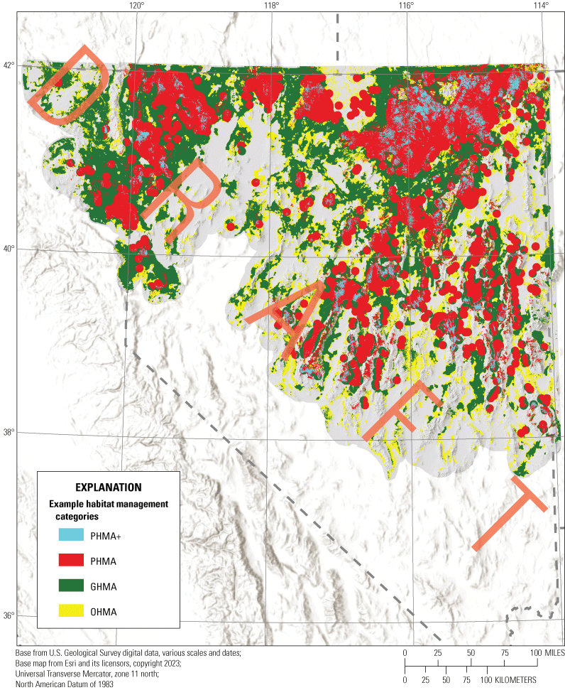
The initial draft (“Draft 1”) of the example habitat management categories delineated for greater sage-grouse (Centrocercus urophasianus) in the western Great Basin region, 2009–21. Draft 1 was reviewed by experts from partner agencies and improved to create the final version (as presented in the main document). Abbreviations: PHMA+, priority+ habitat management area; PHMA, priority habitat management area; GHMA, general habitat management area; OHMA, other habitat management area.
-
1. The models might be improved using newer statistical approaches and additional years of data instead of relying on past outputs from previous models
Draft 1 of the map relied on previously developed outputs that represented spring and summer habitat selection (Coates and others, 2020), whereas outputs for other seasons and life stages were derived from newly developed models. The previous spring and summer habitat selection outputs that were used in the first draft relied on older statistical approaches and telemetry data collected through 2014 (Coates and others, 2020), while the models for other seasons and life stages used a more up-to-date approach within a Bayesian framework and used data through 2021. Therefore, updating the spring and summer habitat selection models and outputs allowed for greater consistency across models, a more rigorous statistical approach described in the “Analysis” sections (see main text), inclusion of an additional 7 years of data, and the adoption of newly available and improved remote sensing products. Implementing models within a Bayesian framework allowed for a more thorough variable selection process, described in “Analysis: Variable Selection,” which provided a strong statistical basis for which variables were included in the final models. Furthermore, release of more accurate remote sensing land cover products (Jones and others, 2018; Rigge and others, 2020; Allred and others, 2021), which our models used for analysis and inference, particularly the development of back-in-time projections of land cover, helped improve the accuracy of model predictions and habitat classifications. For example, two important predictors of selection, annual grass (at the 439-meter [m] scale) and sagebrush cover (at the 1,451-m scale), changed 5 percent and 1 percent, respectively, across the study area between the different versions of remote sensing products and per-pixel changes ranged from an 84-percent decrease to 99-percent increase for annual grass and a 21-percent decrease and 24-percent increase for sagebrush cover. Updating the spring and summer models and maps resulted in a reduction in general habitat (from 54,927 square kilometers [km2] to 21,359 km2), with some changes in the other categories (a decrease of 349 km2 in priority habitat and an increase of 7,863 km2 in other habitat). The reductions in habitat areas were due to the greater accuracy of the newer modeling methodology and improved remote sensing land cover products, whereas previous outputs most likely overestimated general habitat. For example, clear areas of non-habitat, such as playas, were included as general habitat in Draft 1 (questioned as part of our coproduction process), that we addressed by updating the spring and summer outputs with additional data and newly available remote sensing products to improve the final map.
-
2. Apply some form of validation to the habitat selection and survival models to enhance its effectiveness.
Model validation can provide important information on model fit and thus the appropriateness of a model. Updating our modeling approach as described above allowed for the opportunity to incorporate validation for each seasonal and life stage model, which otherwise would not have been possible. Full model validation methodology is described in “Analysis: Models for Habitat Selection” and “Analysis: Models for Survival” and the validation results are described in each section of the “Results” (see main text). Incorporating model validation alone did not change the maps beyond what was described in the previous section with the updates in the spring and summer models. However, including model validation allowed for quantification of how well the models predicted data not used in the original modeling process. Because it is not feasible to monitor all individual sage-grouse, models by necessity are based on samples of individual marked sage-grouse. Model validation, however, provides information on how well a model predicts to unknown individuals and populations. Demonstrating good model fit as described in the “Results” indicates that the models were appropriate and had strong out-of-sample predictive capabilities, thus providing useful representations of sage-grouse habitats across the states of California and Nevada.
-
3. Accounting for movement between seasonal habitats might be important.
The individual habitat selection and survival models implemented here identify areas that are important for sage-grouse during a given season or life stage. However, movement between these areas is likely underrepresented. If important movement corridors are unaccounted for during the modeling and mapping process, management actions may not be properly informed and inadvertently lead to increased fragmentation between important seasonal habitats with population-level impacts. To account for underrepresented connectivity between seasonal habitats, we implemented an additional analysis, described in “Movement and Corridor Analysis” to classify corridors that may connect areas of high abundance with areas identified as source habitat. This analysis provided a novel improvement by incorporating connectivity not addressed using seasonal or life stage models alone and more appropriately captured behavior of sage-grouse. The corridors identified in this analysis were incorporated in the final map as general habitat, increasing that category by 0.18 percent in the final version. In addition, we have provided the corridors as a separate map layer to identify areas that may not represent good seasonal habitat but are important for connectivity between habitats.
-
4. Selected areas predicted to have very low survival were classified as general habitat regardless of whether those areas were occupied causing concern.
The initial set of model rules used for Draft 1 used demographic information to downgrade areas if they had high selection but very low survival (for example, from priority to general habitat) regardless of its location. However, this resulted in small areas (sometimes as small as 900 square meters [m2]) of habitat surrounding some lek locations being classified as general habitat instead of priority habitat. This represented the inherent trade-off between habitat needs during reproduction (lekking versus nesting and brood rearing). Display sites of a lekking species are typically situated in open areas where the displaying individuals can be assessed. However, due to the exposed nature of these sites, they are often risky and typically do not represent good nesting or brood-rearing habitat, as shown in our study where some sites were identified as habitat sinks (areas of loss) for a specific life stage. Nevertheless, both habitats, lek sites and areas for nesting and brood-rearing, are crucial for successful reproduction. Using expert knowledge on sage-grouse behavior and biology, the stewardship group suggested that all selected habitat within the high use category of the abundance and space use index (that is, everything within occupied habitat excluding non-habitat) may be best represented as priority habitat. This update to the map meant that adjustments based on predicted low survival were only applied outside of the high use category of the abundance and space use index to general and other habitat management areas. Within the “low use” of the abundance and space use index any pixels predicted to have high selection but very low survival were downgraded one level (for example, from general to other). This change resulted in the addition of 4,538 km2 of priority habitat that was previously downgraded to general habitat. We have also provided the layer representing areas predicted to have high selection but very low survival (sink habitat; see “Habitat Mapping”) to allow managers to identify these areas for which sage-grouse are selecting but where they experienced reduced demographic performance to provide the opportunity to tailor specific management actions.
-
5. Burned areas should not necessarily be discounted as habitat if they have the potential to recover.
Wildfires were represented in our data through annually time-varying remotely sensed land cover layers representing vegetation cover, such as sagebrush cover, from one year to the next. The time-varying layers represent a vast improvement over static layers, but habitat mapping efforts are then typically based on the most current conditions and do not account for past or future conditions. For example, a recently burned area may be defined as poor quality habitat or non-habitat due to a lack of sagebrush or shrub cover. However, that discounts the potential of that area to recover and may result in all burned areas being considered a loss if they are currently defined as non-habitat. Several partners expressed concern that this could lead to the unnecessary loss of habitat based on current conditions despite their potential to provide future sage-grouse habitat. To address this, we incorporated an additional adjustment, described in “Habitat Recovery Potential in Recently Burned Areas,” to capture pre-fire conditions and allow for recovery potential within occupied habitat. Importantly, we only evaluated pre-fire conditions in fire scars that had recently burned and still had the potential to recover (less than 16 years old; Coates and others, 2016). Overall, this resulted in an addition of 111 km2 of priority habitat to the final map.
-
6. Town boundaries based on U.S. Census data are not inclusive enough to capture outlying developed areas associated with urban areas.
We intentionally did not include anthropogenic features in our models, but we masked out towns, which do not represent habitat for sage-grouse. In Draft 1, to capture recreational activity associated with urban centers we buffered town boundaries based on population size using data on population size and town boundaries from the U.S. Census Bureau. However, this mask did not capture all outlying buildings or new development associated with urban areas. Therefore, we implemented additional steps to improve how towns were represented in the final map. First, we established a buffer distance of 10 kilometers (km) from the boundaries of the initial mask layer based on known distances of development from town centers across Nevada. We then identified any permanent structures using heads-up digitizing based on the National Land Cover Database’s layer representing imperviousness (Dewitz and U.S. Geological Survey, 2021) after excluding roads and Esri’s building footprints layer (https://hub.arcgis.com/maps/esri::microsoft-building-footprints-tiles/about). We then reduced any areas within the digitized boundaries by one level (that is, from priority+ to priority, priority to general, general to other, or other to non-habitat). We also masked all buildings from Esri’s building footprints layer with a 100-m buffer to capture the entire land parcel and other infrastructure associated with the building. The final version therefore better captured the structures associated with population centers. This resulted in reductions of 9 km2 of priority+ habitat, 207 km2 of priority habitat, 175 km2 of general habitat and 363 km2 of other habitat. However, there are multiple options when incorporating information on human infrastructure and end users should take advantage of more localized field data and expertise that could not be incorporated or were not available across the study area to inform management at the local scale.
References Cited
Allred, B.W., Bestelmeyer, B.T., Boyd, C.S., Brown, C., Davies, K.W., Duniway, M.C., Ellsworth, L.M., Erickson, T.A., Fuhlendorf, S.D., Griffiths, T.V., Jansen, V., Jones, M.O., Karl, J., Knight, A., Maestas, J.D., Maynard, J.J., McCord, S.E., Naugle, D.E., Starns, H.D., Twidwell, D., and Uden, D.R., 2021, Improving Landsat predictions of rangeland fractional cover with multitask learning and uncertainty: Methods in Ecology and Evolution, v. 12, no. 5, p. 841–849. [Available at https://doi.org/10.1111/2041-210X.13564.]
Coates, P.S., Brussee, B.E., Ricca, M.A., Severson, J.P., Casazza, M.L., Gustafson, K.B., Espinosa, S.P., Gardner, S.C., and Delehanty, D.J., 2020, Spatially explicit models of seasonal habitat for greater sage-grouse at broad spatial scales—Informing areas for management in Nevada and northeastern California: Ecology and Evolution, v. 10, no. 1, p. 104–118. [Available at https://doi.org/10.1002/ece3.5842.]
Coates, P.S., Ricca, M.A., Prochazka, B.G., Brooks, M.L., Doherty, K.E., Kroger, T., Blomberg, E.J., Hagen, C.A., and Casazza, M.L., 2016, Wildfire, climate, and invasive grass interactions negatively impact an indicator species by reshaping sagebrush ecosystems: Proceedings of the National Academy of Sciences of the United States of America, v. 113, no. 45, p. 12745–12750. [Available at https://doi.org/10.1073/pnas.1606898113.]
Dewitz, J., and U.S. Geological Survey, 2021, National Land Cover Database (NLCD) 2019 Products: U.S. Geological Survey data release v. 2.0, accessed June 13, 2023, at https://www.mrlc.gov/data/nlcd-imperviousness-conus-all-years.
Jones, M.O., Allred, B.W., Naugle, D.E., Maestas, J.D., Donnelly, P., Metz, L.J., Karl, J., Smith, R., Bestelmeyer, B., Boyd, C., Kerby, J.D., and McIver, J.D., 2018, Innovation in rangeland monitoring—Annual, 30 m, plant functional type percent cover maps for US rangelands, 1984–2017: Ecosphere, v. 9, no. 9, 19 p. [Available at https://doi.org/10.1002/ecs2.2430.]
Klinger, T., Dale, V., Sherman, M., McKinney, M., Campbell, J.Y., and Gold, B., 2007, The promise and the challenge of cooperative conservation: Frontiers in Ecology and the Environment, v. 5, no. 2, p. 97–103. [Available at https://doi.org/10.1890/1540-9295(2007)5[97:TPATCO]2.0.CO;2.]
Rigge, M., Homer, C., Cleeves, L., Meyer, D.K., Bunde, B., Shi, H., Xian, G., Schell, S., and Bobo, M., 2020, Quantifying western US rangelands as fractional components with multi-resolution remote sensing and in situ data: Remote Sensing (Basel), v. 12, no. 3, p. 412. [Available at https://doi.org/10.3390/rs12030412.]
Appendix 4. Results of Variable Reduction Analyses
Table 4.1.
Candidate landscape covariates for habitat selection models of nesting greater sage-grouse (Centrocercus urophasianus) in the western Great Basin region, 2009–21.[Scales were selected from a preliminary Bayesian latent indicator variable selection procedure, where scales with a greater proportion of the posterior distribution were selected over other grouped covariates. Only covariates in groups with proportion of Markov Chain Monte Carlo iterations where the indicator variable equaled 1 (w)>0.50 were carried into final models. Abbreviations: m, meters; RAP, Rangeland Analysis Platform; RCMAP, Rangeland Condition Monitoring Assessment and Projection; HLI, heat load index; TRASP, transformed aspect; TPI, topographic position index; NA, not applicable]
Table 4.2.
Candidate landscape covariates for nest survival models of greater sage-grouse (Centrocercus urophasianus) in the western Great Basin region, 2009–21.[Scales were selected from a preliminary Bayesian latent indicator variable selection procedure, where scales with a greater proportion of the posterior distribution were selected over other grouped covariates. Only covariates in groups with proportion of Markov Chain Monte Carlo iterations where the indicator variable equaled 1 (w)>0.50 were carried into final models. Abbreviations: m, meters; RAP, Rangeland Analysis Platform; RCMAP, Rangeland Condition Monitoring Assessment and Projection; HLI, heat load index; TRASP, transformed aspect; TPI, topographic position index; NA, not applicable]
Table 4.3.
Candidate landscape covariates for habitat selection models of early brood-rearing greater sage-grouse (Centrocercus urophasianus) in the western Great Basin region, 2009–21.[Scales were selected from a preliminary Bayesian latent indicator variable selection procedure, where scales with a greater proportion of the posterior distribution were selected over other grouped covariates. Only covariates in groups with proportion of Markov Chain Monte Carlo iterations where the indicator variable equaled 1 (w)>0.50 were carried into final models. Abbreviations: m, meters; RAP, Rangeland Analysis Platform; RCMAP, Rangeland Condition Monitoring Assessment and Projection; HLI, heat load index; TRASP, transformed aspect; TPI, topographic position index; NA, not appliable; ×, multiplied by]
Table 4.4.
Candidate landscape covariates for survival models of early brood-rearing greater sage-grouse (Centrocercus urophasianus) in the western Great Basin region, 2009–21.[Scales were selected from a preliminary Bayesian latent indicator variable selection procedure, where scales with a greater proportion of the posterior distribution were selected over other grouped covariates. Only covariates in groups with proportion of Markov Chain Monte Carlo iterations where the indicator variable equaled 1 (w)>0.50 were carried into final models. Abbreviations: m, meters; RAP, Rangeland Analysis Platform; RCMAP, Rangeland Condition Monitoring Assessment and Projection; HLI, heat load index; TRASP, transformed aspect; TPI, topographic position index; NA, not applicable; ×, multiplied by]
Table 4.5.
Candidate landscape covariates for habitat selection models of late brood-rearing greater sage-grouse (Centrocercus urophasianus) in the western Great Basin region, 2009–21.[Scales were selected from a preliminary Bayesian latent indicator variable selection procedure, where scales with a greater proportion of the posterior distribution were selected over other grouped covariates. Only covariates in groups with proportion of Markov Chain Monte Carlo iterations where the indicator variable equaled 1 (w)>0.50 were carried into final models. Abbreviations: m, meters; RAP, Rangeland Analysis Platform; RCMAP, Rangeland Condition Monitoring Assessment and Projection; HLI, heat load index; TRASP, transformed aspect; TPI, topographic position index; NA, not applicable; ×, multiplied by]
Table 4.6.
Candidate landscape covariates for survival models of late brood-rearing greater sage-grouse (Centrocercus urophasianus) in the western Great Basin region, 2009–21.[Scales were selected from a preliminary Bayesian latent indicator variable selection procedure, where scales with a greater proportion of the posterior distribution were selected over other grouped covariates. Only covariates in groups with proportion of Markov Chain Monte Carlo iterations where the indicator variable equaled 1 (w)>0.50 were carried into final models. Abbreviations: m, meters; RAP, Rangeland Analysis Platform; RCMAP, Rangeland Condition Monitoring Assessment and Projection; HLI, heat load index; TRASP, transformed aspect; TPI, topographic position index; NA, not applicable; ×, multiplied by]
Table 4.7.
Candidate landscape covariates for habitat selection models of greater sage-grouse (Centrocercus urophasianus) in the spring in the western Great Basin region, 2009–21.[Scales were selected from a preliminary Bayesian latent indicator variable selection procedure, where scales with a greater proportion of the posterior distribution were selected over other grouped covariates. Only covariates in groups with proportion of Markov Chain Monte Carlo iterations where the indicator variable equaled 1 (w)>0.50 were carried into final models. Abbreviations: m, meters; RAP, Rangeland Analysis Platform; RCMAP, Rangeland Condition Monitoring Assessment and Projection; HLI, heat load index; TRASP, transformed aspect; TPI, topographic position index; NA, not applicable]
Table 4.8.
Candidate landscape covariates for habitat selection models of greater sage-grouse (Centrocercus urophasianus) in the summer in the western Great Basin region, 2009–21.[Scales were selected from a preliminary Bayesian latent indicator variable selection procedure, where scales with a greater proportion of the posterior distribution were selected over other grouped covariates. Only covariates in groups with proportion of Markov Chain Monte Carlo iterations where the indicator variable equaled 1 (w)>0.50 were carried into final models. Abbreviations: m, meters; RAP, Rangeland Analysis Platform; RCMAP, Rangeland Condition Monitoring Assessment and Projection; HLI, heat load index; TRASP, transformed aspect; TPI, topographic position index; NA, not applicable; ×, multiplied by]
Table 4.9.
Candidate landscape covariates for habitat selection models of greater sage-grouse (Centrocercus urophasianus) in the winter in the western Great Basin region, 2009–21.[Scales were selected from a preliminary Bayesian latent indicator variable selection procedure, where scales with a greater proportion of the posterior distribution were selected over other grouped covariates. Only covariates in groups with proportion of Markov Chain Monte Carlo iterations where the indicator variable equaled 1 (w)>0.50 were carried into final models. Abbreviations: m, meters; RAP, Rangeland Analysis Platform; RCMAP, Rangeland Condition Monitoring Assessment and Projection; HLI, heat load index; TRASP, transformed aspect; TPI, topographic position index; NA, not applicable]
Appendix 5. Mapping Habitat Suitability with the Abundance and Space Use Index
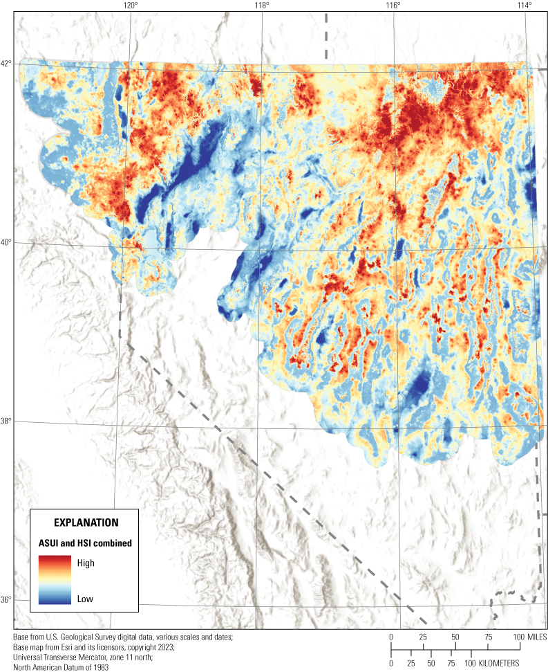
The metric combining habitat suitability with the abundance and space use index (ASUI) for greater sage-grouse (Centrocercus urophasianus) in the western Great Basin region, 2009–21. The habitat suitability index (HSI) combined selection and survival maps during phenological seasons and life stages.
Datum
Horizontal coordinate information is referenced to the North American Datum of 1983 (NAD 83).
Elevation, as used in this report, refers to distance (meters) above the vertical datum.
Abbreviations
ASUI
abundance and space use index
BLISS
Bayesian latent indicator scale selection
BLM
Bureau of Land Management
DSR
daily survival rate
GHMA
General habitat management area
GIS
geographic information system
GPS
Global Positioning System
HLI
heat load index
LCP
least-cost path
MCMC
Markov Chain Monte Carlo
OHMA
Other habitat management area
PHMA
Priority habitat management area
PHMA+
Priority+ habitat management area
RAP
Rangeland Analysis Platform
RCMAP
Rangeland Condition Monitoring Assessment and Projection
RSF
resource selection function
TPI
topographic position index
TRASP
transformed aspect
UD
utilization distribution
USGS
U.S. Geological Survey
For more information concerning the research in this report, contact the
Director, Western Ecological Research Center
U.S. Geological Survey
3020 State University Drive East
Sacramento, California 95819
https://www.usgs.gov/centers/werc
Publishing support provided by the U.S. Geological Survey
Science Publishing Network, Sacramento Publishing Service Center
Disclaimers
Any use of trade, firm, or product names is for descriptive purposes only and does not imply endorsement by the U.S. Government.
Although this information product, for the most part, is in the public domain, it also may contain copyrighted materials as noted in the text. Permission to reproduce copyrighted items must be secured from the copyright owner.
Suggested Citation
Milligan, M.C., Coates, P.S., O’Neil, S.T., Brussee, B.E., Chenaille, M.P., Friend, D., Steele, K., Small, J.R., Bowden, T.S., Kosic, A.D., and Miller, K., 2024, Greater sage-grouse habitat of Nevada and northeastern California—Integrating space use, habitat selection, and survival indices to guide areas for habitat management: U.S. Geological Survey Open-File Report 2024–1018, 70 p., https://doi.org/10.3133/ofr20241018.
ISSN: 2331-1258 (online)
Study Area
| Publication type | Report |
|---|---|
| Publication Subtype | USGS Numbered Series |
| Title | Greater sage-grouse habitat of Nevada and northeastern California—Integrating space use, habitat selection, and survival indices to guide areas for habitat management |
| Series title | Open-File Report |
| Series number | 2024-1018 |
| DOI | 10.3133/ofr20241018 |
| Publication Date | March 22, 2024 |
| Year Published | 2024 |
| Language | English |
| Publisher | U.S. Geological Survey |
| Publisher location | Reston, VA |
| Contributing office(s) | Western Ecological Research Center |
| Description | Report: viii, 70 p.: Data Release |
| Country | United States |
| State | California, Idaho, Nevada |
| Online Only (Y/N) | Y |