Special Contributing Area Loading Program user’s manual

Henry F. Doyle; Marian M. Domanski

doi:10.3133/ofr20241021

Special Contributing Area Loading Program User’s Manual

Open-File Report 2024-1021

Prepared in cooperation with the U.S. Army Corps of Engineers

By: Henry F. Doyle and Marian M. Domanski

https://doi.org/10.3133/ofr20241021

Links

Document: Report (4.0 MB pdf) , HTML , XML
Software Release: USGS software release —SCALP (Special Contributing Area Loading Program, ver. 1.0.0)
Download citation as: RIS | Dublin Core

Acknowledgments

This work was funded by the U.S. Army Corps of Engineers.

Introduction

The Special Contributing Area Loading Program (SCALP) is a hydrologic routing program that simulates reservoir routing through a linear-reservoir-in-series method. The Java version of SCALP (Domanski and Doyle, 2023) was developed to replicate and replace the functionality of an older version of the program written in Fortran. SCALP models flow through three reservoirs in series using an input runoff depth time series and information describing the hydrologic characteristics and sanitary flow for one or more land areas within a basin, supplied by the user. Each basin is herein referred to as a “Special Contributing Area” (SCA); the SCAs are a central concept in SCALP. Although flow through each SCA is routed separately, the user may simulate multiple SCAs in a batch simulation. The outputs of SCALP include information about flows through and overflows from the three reservoirs in the series.

SCALP simulates reservoir routing through a linear-reservoir-in-series method. Each SCA contains hydrologic characteristics pertaining to its three reservoirs in series, land areas within the SCA, and sanitary flows from the population that contribute to the basin. Three components of inflow are defined for each SCA: stormwater flow, sewer infiltration, and sanitary flow. Each land area, also referred to as a “land segment,” contains three tributary area types (pervious, impervious, and subsurface) and requires three runoff depth time series as inputs (overland flow runoff [OLFRO], impervious runoff [IMPRO], and subsurface runoff [SUBRO]). Using the three tributary area types and the three input runoff depth time series, the stormwater flow and sewer infiltration are computed for each land segment. Stormwater flow time series are computed for each time step by

INFLO

=

OLFRO

×

PA

+

IMPRO

×

IMPA

,

(1)

where

INFLO: is the stormwater flow, in cubic feet per second;
OLFRO: is the overland runoff, in inches per hour;
PA: is the pervious area, in square miles;
IMPRO: is the impervious runoff, in inches per hour; and
IMPA: is the impervious area, in square miles.

Sewer infiltration time series are computed for each time step by

INFIL

=

SUBRO

×

SUBA

,

(2)

where

INFIL: is the stormwater flow,
SUBRO: is the subsurface runoff, and
SUBA: is the subsurface area.

The total stormwater and sewer infiltration flow from an SCA is the sum of the respective flow time series among the land segments within the SCA. Finally, sanitary flow is computed for each time step by

SANIT

=

PE

×

HFF

×

WFF

×

MFF

,

(3)

where

SANIT: is the sanitary flow,
PE: is the population equivalence,
HFF: is the hourly flow factor,
WFF: is the weekly flow factor, and
MFF: is the monthly flow factor.

Flows from each source (stormwater, sewer infiltration, and sanitary) are tracked through the routing process by the proportion of the contribution to total sewer inflow (the sum of the three components).

For each SCA, the stormwater, sewer infiltration, and sanitary flows are routed through three sewers represented in SCALP by three linear reservoirs in series. The three sewers are herein referred to as “lateral,” “submain,” and “main” sewers, where the lateral sewer is first, the submain sewer is second, and the main sewer is third in the series. Each sewer is characterized by a routing coefficient, maximum flow, a stop store flag, and split flow. The routing coefficient is the proportionality constant of the linear relation between reservoir storage and outflow determined empirically for each reservoir. The maximum flow parameter is the maximum volume of flow that can be routed through a sewer; any volume of flow exceeding the maximum flow is either lost from the sewer system or stored until it can be released, and the stop store flag determines this behavior. The usage of the stop store flag parameter is described in further detail in the “Special Contributing Area Input Block” section. The split flow parameter defines sewer overflow; flows through a sewer exceeding the split flow are routed to sewer overflow, and flows less than the split flow value are routed through the sewer system. Outflows from the lateral reservoir are routed to the submain reservoir, and outflows from the submain reservoir are routed to the main reservoir. The time series of outflow from the main sewer and overflow from the system are written to a Hydrologic Engineering Center-Data Storage System (HEC–DSS) file, and qualitative descriptions of the SCALP routing process are written to a text-based log file.

Inputs to SCALP include runoff depth time series and a user-defined text file. The input runoff depth time series must be formatted as an HEC–DSS file as described in the “Hydrologic Time Series Input” section, and the text file must follow the format outlined in the “Special Contributing Area Inputs” section. Similarly, the outputs of SCALP are outflow time series contained in an HEC–DSS file and an output log contained in a text file; each is described in the “Model Results” section. Instructions to run single and batch SCALP simulations are provided in the “Installation” section.

Reservoir Routing

For each of the three linear reservoirs in series, SCALP determines the outflow from the reservoir as a function of the inflow to the reservoir and the reservoir’s routing coefficient. A fourth-order Runge-Kutta (RK4) method (Runge, 1895; Kutta, 1901) is implemented in SCALP, and the equations governing outflow from a linear reservoir using this method are described in this section.

Linear Reservoir

The time rate of change of the storage of water in a system is related to the net inflow and outflow of water by (Chow and others, 1988)

\frac{d S}{d t} = I - Q

,

(4)

where

S: is the storage, or volume, of water in a system, in cubic feet;
t: is time, in seconds;
I: is the net inflow to the system, in cubic feet per second; and
Q: is the net outflow from the system, in cubic feet per second.

A linear reservoir is defined as a reservoir that has a storage that is directly proportional to the outflow (Chow and others, 1988),

S

=

KQ

,

(5)

where

K: is the storage coefficient of the reservoir, in seconds (Pedersen and others, 1980).

Substituting equation 5 into equation 4 and dividing through by K yields equation 6, which is the governing equation for the linear-reservoir model.

\frac{d Q}{d t} = \frac{1}{K} I - \frac{1}{K} Q

.

(6)

Because the inflows are known, equation 6 is a linear ordinary differential equation (ODE) for Q as a function of t. SCALP routes flow from an SCA into a sewer system modeled as three linear reservoirs in series. Although a system of linear reservoirs in series may be solved as a system of three ODEs, this is not possible in SCALP because of the nonlinear behavior of the maximum outflow and split flow features described in the “Introduction” section. Thus, SCALP numerically integrates equation 6 for each reservoir using the RK4 method; this is described further in the next section.

Integration Methods

SCALP uses the RK4 integration method to solve the system of three ODEs for the three linear reservoirs in series. First, a pass-through integrator is defined, which sets the outflow from the reservoir equal to the inflow at each time step,

Q_n

=

I_n

,

(7)

for n=0, 1, 2, 3, …

This integration method is used for reservoirs in which the storage coefficient K is equal to zero; that is, there is no delay between flow entering the reservoir to flow leaving the reservoir.

For a reservoir with a nonzero storage coefficient K, a Runge-Kutta method is used. A first-order Runge-Kutta method is Euler’s method; in this approach, the rate of change of Q is assumed to follow the function for Q closely for a small timestep (Euler, 1768),

Q_n₊₁

=

Q_n

+Δ

t

⋅

f

(

t_n

,

Q_n

),

(8)

for n=0, 1, 2, 3, …, where

Δt: is the timestep, in seconds; and
f: is the time rate of change of Q, determined by equation 6.

Building off the Euler’s method for a first-order integration, the RK4 method presents a fourth-order solution (Runge, 1895; Kutta, 1901),

Q_{n = 1} = Q_{n} + \frac{Δ t}{6} (k_{1} + 2 k_{2} + 2 k_{3} + k_{4})

(9)

where

k_{1} = f (t_{n}, Q_{n})

,

k_{2} = f (t_{n} + \frac{Δ t}{2}, Q_{n} + k_{1} \cdot \frac{Δ t}{2})

,

k_{3} = f (t_{n} + \frac{Δ t}{2}, Q_{n} + k_{2} \cdot \frac{Δ t}{2})

, and

k_{4} = f (t_{n} + Δ t, Q_{n} + k_{3} \cdot Δ t)

;

for n=0, 1, 2, 3, …, where

Δt: is the timestep, in seconds; and
f: is the time rate of change of Q, determined by equation 6.

The Euler method and the RK4 method are both Runge-Kutta methods: they select an interval, compute a representative time rate of change of Q using the value of Q at the start of the interval, and then determine the value of Q at the end of the interval. These methods assume that the value of Q at the end of the interval is on the actual (unknown) curve for Q, which can then be used as the starting value for the next timestep. The approximated curve does not perfectly follow the actual (unknown) curve for either method; however, given a small timestep and a finite interval of computation, the difference between the approximated curve and the actual (unknown) curve can be minimized. The Euler method is a simple approximation; because the RK4 method improves the accuracy of the approximated curve with low additional computational cost, it is implemented in SCALP.

Usage

SCALP is written in Java and depends on a Java library developed by the U.S. Army Corps of Engineers Hydrologic Engineering Center to operate with the HEC–DSS input and outputs. This section details the installation process for SCALP, how to run a SCALP simulation, and the inputs that are required (a runoff depth time series and a user-defined text file).

Installation

The SCALP executable Java Archive file and source code in a compressed ZIP file can be downloaded from the U.S. Geological Survey Source Code Archive (https://code.usgs.gov/water/SCALP/-/releases; Domanski and Doyle, 2023). To run SCALP simulations, first download and save the directory “scalp-1.0.0-jre-win_amd64.zip” from the source code archive. Then, extract the contents of the compressed directory to a new folder and save the desired input runoff depth time series and user-defined text file to this folder (refer to “Hydrologic Time Series Input” and “Special Contributing Area Inputs” sections, respectively). Then, run the commands in Windows Command Prompt, shown in figure 1 for a single simulation and figure 2 for multiple (batch) simulations, using path names as follows: “path-to-lib32-or-lib64” is the path to the “lib32” or “lib64” directory being used (users can use the “lib32” or “lib64” directories included in the downloaded files), “path-to-jre-or-jdk” is the path to the directory of the Java installation (users can use the “jre” directory included in the downloaded files), “path-to-scalp-jar.jar” is the path to the executable SCALP Java Archive file downloaded from the archive, “path-to-input-runoff-depth-time-series.dss” is the path to the input runoff depth time series as an HEC–DSS file, “path-to-output-outflow-time-series.dss” is the path at which SCALP will save the output outflow time series as an HEC–DSS file, “input.txt” is the path to the input user-defined text file, and “output.txt” is the output log as a text file. Note that for batch simulations, different input and output files can be specified for each simulation. The outputs of a SCALP simulation are described in further detail in the “Model Results” section.

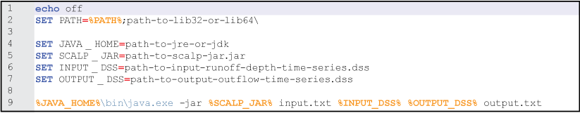
A total of nine lines show command line arguments in Windows Command Prompt. — Figure 1.
Example command line arguments used to run a single Special Contributing Area Loading Program simulation in Windows Command Prompt.

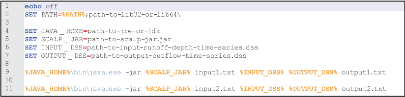
A total of 11 lines show command line arguments in Windows Command Prompt. — Figure 2.
Example command line arguments used to run multiple Special Contributing Area Loading Program simulations that share the same input runoff depth time series file and output outflow time series file, in Windows Command Prompt.

Hydrologic Time Series Input

One of the inputs to SCALP is a runoff depth time series formatted as an HEC–DSS file. Hydrologic Engineering Center-Data Storage System Visual Utility Engine (HEC–DSSVue), a Java-based program designed for working with data in an HEC–DSS database file, was used to visualize the example SCALP HEC–DSS input file described in this section. Downloads and more information on HEC–DSSVue are available at https://www.hec.usace.army.mil/software/hec-dssvue/.

The input runoff depth time series file must be formatted as an HEC–DSS database file. For each land segment used in the SCAs of an input file, the runoff depth input file must contain three time series: IMPRO, OLFRO, and SUBRO depth. An example input runoff depth time series that contains the appropriate time series for four land segments is shown in figure 3. The HEC–DSS path parts are shown in figure 3 as the table headings; parts A, B, and F are read by SCALP, and each time series must have a unique combination of these parts. Although part D is not used by SCALP, it must contain dates in “DDMMMYYYY” format (DD is day; MMM is month; YYYY is year) to be compatible with the javaHeclib dependency, as shown in figure 3.

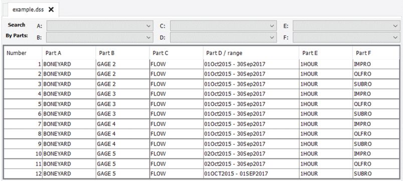
A table with 12 entries shows input path parts in Hydrologic Engineering Center-Data
Storage System Visual Utility Engine. — Figure 3.
Example input runoff depth time series file viewed in Hydrologic Engineering Center-Data Storage System Visual Utility Engine.

Each time series in the input HEC–DSS file should contain 1-hour average runoff data reported at the end of each hour, in inches. An example SUBRO time series for the period ranging from October 1, 2015, to September 30, 2017, is shown in figure 4, plotted and tabulated in HEC–DSSVue.

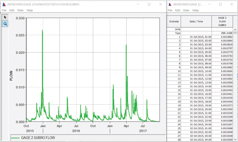
A time series plot and table show subsurface runoff flow over a 2-year period for
gage 2 in Hydrologic Engineering Center-Data Storage System Visual Utility Engine. — Figure 4.
Example subsurface runoff depth time series plotted and tabulated in Hydrologic Engineering Center-Data Storage System Visual Utility Engine.

Special Contributing Area Inputs

Information pertaining to each SCA that the user wishes to simulate must be contained in a user-specified text input file. SCALP requires that the information be formatted according to the format presented in this section; SCALP will not complete a successful simulation if the format is not followed. The user input file consists of three input blocks: the “watershed” input block contains the start and end date of the simulation and information about land segments, the “sanitary” input block contains information about sanitary flow, and the “SCA” input block contains information about each SCA to be simulated. A user input file contains one type of each input block; figure 5 shows an example input file in its entirety, and each input block is described in further detail in this section. Comment lines, which begin with +++, are ignored by SCALP and do not affect simulations. In the following figure and tables, spaces are represented by a middle dot character.

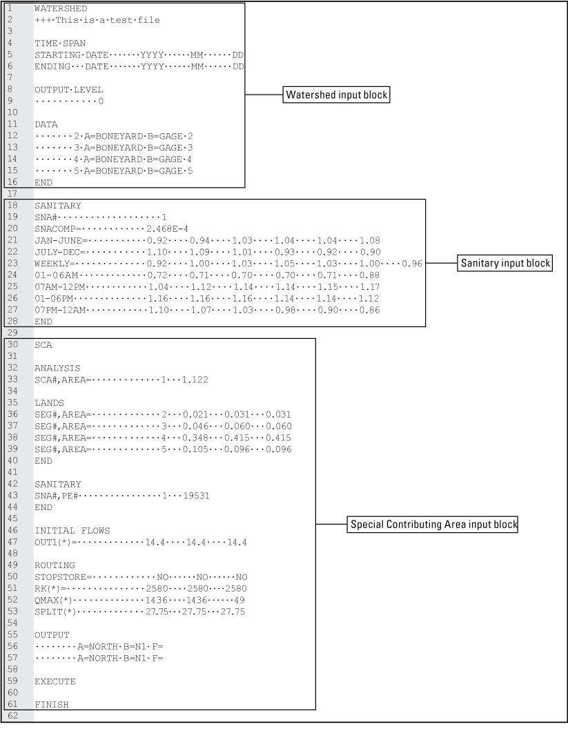
A total of 62 lines show user-defined text inputs. — Figure 5.
Example user-defined text input file. Spaces are represented by a middle dot character.

The SCALP user input file contains information for simulating runoff through SCAs. The current version of SCALP is designed to work with the legacy user input file format, which uses Fortran style formatting. The convention specifies the number of fields, the field type, and the character width of the field; table 1 identifies each field type indicator and its type. For instance, “3I8” indicates three fields on one line, each with a width of eight characters, that are parsed as three distinct integers. If the number of fields is unspecified, it is understood to be one. For example, “A9” indicates one field, parsed as characters, with a width of nine characters. If the field width is unspecified, the number of characters is understood to be one; for example, “16X” indicates 16 fields, which are ignored, each with a character width of 1. Multiple field descriptions, separated by a comma, can be used on a single line. For example, “I8,A72” describes two fields on one line. The first field is parsed as 1 integer with a character width of 8, and the second field is parsed as characters and has a field width of 72.

Table 1.

Field type indicators for user input file formatting.

Table 1. Field type indicators for user input file formatting.
Type indicator	Type
A	Character
I	Integer
F	Floating point
E	Exponential
X	Ignored

Watershed Input Block

The watershed input block contains information about the start and end dates of the simulation and the land segments used in the file’s SCAs. The watershed input block in figure 5 is contained in lines 1–16, and table 2 details the formatting of each section and element in the watershed input block. In tables 2–4, the block, section, and element columns contain example text for the input file, and the format and comment columns describe the text and its format. Numerical values used in the element column are representative and should reflect the parameters of each specific simulation.

The “WATERSHED” keyword starts the watershed input block, and “+++” denotes an optional comment line that is ignored by the program. For the “TIME SPAN” element, only one starting date and one ending date should be specified, and these dates should be encompassed within the date range of the hydrologic time series input. The “OUTPUT LEVEL” is a feature of the legacy program in Fortran and is not used in this version of SCALP; however, these lines must be included to accommodate the legacy input file format. Lastly, the “DATA” section contains land segment numbers and corresponding HEC–DSS paths of the input runoff time series. All land segments used in the SCAs for this file must be specified in this “DATA” section; multiple land segment numbers can be specified by separating each number onto a new line. In each line defining a land segment, the first field, parsed as an integer, must be a unique land segment number. The second field, parsed as a character string, is a short form of the corresponding HEC–DSS path identifying the A and B fields of the path. The HEC–DSS paths of the time series correspond to the paths of records contained in the input HEC–DSS file, which is specified on the command line call of SCALP. SCALP expands the short form of the path to three full HEC–DSS paths that identify the IMPRO, OLFRO, and SUBRO runoffs as part F of the HEC–DSS path. The example in table 2 lists a land segment that has a number of 2 and HEC–DSS path part A of “BONEYARD” and part B of “GAGE 2.” The watershed input block must end with the “END” keyword.

Table 2.

Watershed input block formatting.

^{[--, no data or not applicable; +++, denotes optional comment line; ·, denotes a space;
HEC–DSS, Hydrologic Engineering Center-Data Storage System]}

Table 2. Watershed input block formatting.
Block	Section	Element	Format	Comment
WATERSHED	--	--	A9	Start of watershed input block
--	+++…	--	A*	Comment line within file
--	TIME·SPAN	--	A9	Start and end dates of simulation
--	--	STARTING·DATE·······2015······10······02	16X,3I8	Start year, month, day
--	--	ENDING···DATE·······2017······09······30	16X,3I8	End year, month, day
--	OUTPUT·LEVEL		A12	Set log file table level
--	--	···········0	11X,I1	Output level: 0: echo user file data (default) 1: daily averages + echo 2: hourly averages + echo
--	DATA	--	A9	Start of land segment numbers and input HEC–DSS paths
--	--	·······2·A=BONEYARD·B=GAGE·2	I8,A72	Segment numbers and input path using one of two input styles: 1: Complete HEC–DSS path 2: HEC–DSS path parts as A= B=
--	END	--	A3	End of watershed input block

Sanitary Input Block

The sanitary input block consists of one or more sanitary information sets that define the creation of sanitary flow time series. SCALP uses sanitary information sets to compute a time-varying sanitary flow per person, which is then converted to total sanitary flow for the population of an SCA. The sanitary input block is contained in lines 18–28 in figure 5 for a single sanitary information set, and table 3 contains details for the formatting of the sanitary input block.

Table 3.

Sanitary input block formatting.

^{[Times are given in military time. --, no data or not applicable; ·, denotes a space]}

Table 3. Sanitary input block formatting.
Block	Element	Format	Comment
SANITARY	--	A8	Start of sanitary input block
--	SNA#···················1	A3,13X,I8	Number of sanitary flow information set
--	SNACOMP=············2.468E-4	16X,E20.5	Sanitary flow per person, in cubic feet per second
--	JAN-JUNE=···········0.92····0.94····1.03····1.04····1.04····1.08	16X,6F8.0	Monthly sanitary flow factors for January through June
--	JULY-DEC=···········1.10····1.09····1.01····0.93····0.92····0.90	16X,6F8.0	Monthly sanitary flow factors for July through December
--	WEEKLY=·············0.93····1.00····1.03····1.05····1.03····1.00····0.96	16X,7F8.0	Weekly sanitary flow factors for Sunday through Saturday
--	01-06AM=············0.72····0.71····0.70····0.70····0.71····0.88	16X,6F8.0	Hourly sanitary flow factors for 0100 to 0600 hours each day
--	07AM-12PM=··········1.04····1.12····1.14····1.14····1.15····1.17	16X,6F8.0	Hourly sanitary flow factors for 0700 to 1200 hours each day
--	01-06PM=············1.16····1.16····1.16····1.14····1.14····1.12	16X,6F8.0	Hourly sanitary flow factors for 1300 to 1800 hours each day
--	07PM-12AM=··········1.10····1.07····1.03····0.98····0.90····0.86	16X,6F8.0	Hourly sanitary flow factors for 1900 to 2400 hours each day
END	--	A3	End of sanitary input block

The “SANITARY” keyword starts the sanitary input block, followed by sanitary information sets. Each sanitary information set defined in an input text file must have a unique identifying number specified on the line that begins with the “SNA#” keyword. The next line contains the sanitary flow per person in the SCA expressed as a scientific number. The following two lines contain monthly sanitary flow factors: the first line contains the flow factors for January through June, and the second line contains the flow factors for July through December. The line after the monthly flow factors contains the weekday flow factors; seven fields contain the weekday flow factors for Sunday through Saturday. The next four lines contain hourly flow factors for each hour of the day (listed as the ending time; for example, 0100 refers to 0000 to 0100): the first line, “01–06AM,” contains the flow factors for 0100 through 0600 hours, the second line, “07AM–12PM,” for 0700 through 1200 hours, the third line, “01–06PM,” for 1300 through 1800 hours, and the last line, “07PM–12AM,” for 1900 through 2400 hours. If multiple sanitary information sets are specified, the next line begins the next information set with the “SNA#” keyword and the unique set number, followed by the flow factors. The sanitary input block ends with the “END” keyword, which must be present.

Special Contributing Area Input Block

Finally, the SCA input block is the last block in the user input file. This block contains information for each SCA in the simulation pertaining to the sewer inflows and characteristics. In the example in figure 5, the SCA input block is contained in lines 30–61, and table 4 details the formatting necessary for the SCA input block. The SCA input block begins with the keyword “SCA” and must contain one or more SCA definitions. The definition of an SCA begins with the keyword “ANALYSIS” and ends with the keyword “EXECUTE”; multiple SCAs can be separated by new lines, and the “FINISH” keyword indicates to SCALP that there are no more SCAs to simulate. An SCA is defined by a unique SCA number and area, land segments, sanitary information set numbers and SCA population, reservoir routing characteristics, and output time series file location.

Immediately after the “ANALYSIS” keyword, the SCA number and area fall on a single line beginning with the keyword “SCA#,AREA=” and containing a unique SCA number and total SCA area. The SCA area is a floating-point number that represents the total SCA area, in square miles. Land segments are specified for the SCA beginning with the “LANDS” keyword and ending with the “END” keyword. Each line in the “LANDS” section must contain the unique identifier for the land segment (which must also be present in the watershed input block) and three floating-point numbers that correspond to the impervious, pervious, and subsurface tributary areas, in square miles. Multiple land segments can be specified by separating each land segment by new lines. The sanitary flow contribution section is denoted by the “SANITARY” keyword and ends with another “END” keyword. For each sanitary flow contribution for the SCA, a line beginning with “SNA#,PE#” contains the unique sanitary information set number (which must be present in the sanitary input block) and the total population equivalent of the sanitary flow contribution, in number of people. Multiple sanitary flow contributions may be specified, separating each by a new line.

The routing scheme that SCALP implements uses three linear reservoirs in series that represent the three sewers: lateral, submain, and main. Routing information is specified for each sewer type, including initial flows, an overflow indicator, routing constants, maximum flow, and split flow. These characteristics are defined in the routing information section, which begins with the “INITIAL FLOWS” keyword, and all the following fields specify characteristics for the three sewers—lateral, submain, and main—respectively. Initial flows through each sewer are specified on the line beginning with the keyword “OUT1(*)=,” in cubic feet per second. This line is followed by the “ROUTING” keyword. Next, the line containing the “STOPSTORE=” keyword indicates, for each reservoir, whether excess flows are to be stored or lost from the sewer system. “NO” indicates that excess flows are to be stored; “YES” indicates that excess flows are to be lost from the system entirely. The line starting with the keyword “RK(*)=” defines the routing constants for each reservoir, in seconds. Then, the lines starting with “QMAX(*)” and “SPLIT(*)” define the maximum flow and split flow through each reservoir, respectively, whose functionalities are defined in the “Introduction” section.

The “OUTPUT” section of the SCA input block contains summation indicators and corresponding HEC–DSS paths of output sewer flows and overflows. The first field specifies the summation indicator, which is not used and is only included to support the legacy input text file format. The second field, parsed as a character string, is a short form of the corresponding HEC–DSS path identifying the A, B, and F fields of the path. Part F of the HEC–DSS path is not necessary to specify; SCALP expands the short form of the path to three full HEC–DSS paths that identify the IMPRO, OLFRO, and SUBRO runoff as part F. Each defined SCA ends with the “EXECUTE” keyword, and the SCA input block must end with the “FINISH” keyword.

Table 4.

Special Contributing Area input block formatting.

^{[SCA, Special Contributing Area; --, no data or not applicable; HEC–DSS, Hydrologic
Engineering Center-Data Storage System]}

Table 4. Special Contributing Area input block formatting.
Block	Section	Element	Format	Comment
SCA	--	--	A3	Beginning of SCA input block
--	ANALYSIS	--	A8	Header for SCA information
--	--	SCA#,AREA=·············1···1.122	A3,13X,I8,F8.0	SCA number and total SCA area, in square miles
--	LANDS	--	A5	Start of lands section
--	--	SEG#,AREA=·············2···0.021···0.031···0.031	A3,13X,I8,3F8.0	Segment number and areas of impervious, pervious, and subsurface tributary to SCA sewers, in square miles
--	END	--	A3	End of lands section
--	SANITARY	--	A8	Start of sanitary information
--	--	SNA#,PE=···············1···19531	A3,13X,I8,F8.0	Sanitary information set number and population equivalent, in number of people
--	END	--	A3	End of sanitary information
--	INITIAL·FLOWS	--	A13	Start of initial flows
--	--	OUT1(*)=············14.4····14.4····14.4	16X,3F8.0	Initial flows in lateral, submain, and main sewers, in cubic feet per second
--	ROUTING	--	A7	Start of routing information
--	--	STOPSTORE=············NO······NO······NO	16X,3(5X,A3)	Indicator for lateral, submain, and main excess flows to be lost from SCA (YES/NO)
--	--	RK(*)=··············2580····2580····2580	16X,3F8.0	Routing constants for lateral, submain, and main sewers, in seconds
--	--	QMAX(*)·············1436····1436······49	16X,3F8.0	Maximum flows in lateral, submain, and main sewers, in cubic feet per second
--	--	SPLIT(*)···········27.75···27.75···27.75	16X,3F8.0	Cutoff flow level for lateral, submain, and main sewers, in cubic feet per second
--	OUTPUT	--	A6	Start of output HEC–DSS paths
--	--	········A=NORTH·B=N1·F=	I8,A72	Summation indicator and HEC–DSS path for total, inflow, infiltration, and sanitary treatment plant flows as HEC–DSS path or A=, B=, F=
--	--	········A=NORTH·B=N1·F=	I8,A72	Summation indicator and HEC–DSS path for total, inflow, infiltration, and sanitary treatment plant overflows as HEC–DSS path or A=, B=, F=
--	EXECUTE	--	A7	Line to start execution of the SCA simulation
FINISH	--	--	A9	End of SCALP run

Model Results

SCALP outputs a hydrologic time series and a descriptive text file at the end of each simulation. This section describes how to read and interpret these results.

Hydrologic Time Series Output

Similar to the runoff depth time series input, the output outflow time series from a SCALP simulation is formatted as an HEC–DSS database file. For each SCA simulated, eight time series are generated by SCALP; figure 6 shows the hydrologic output viewed in HEC–DSSVue for an example simulation with a single SCA. For files with multiple SCAs, the output files for each SCA can be identified by the path parts A and B specified in the SCA input block in the input text file, as described in the “Special Contributing Area Inputs” section. Part F for each time series contains a prefix and a suffix: the prefix indicates whether it is the sewer overflow (“OVF” in fig. 6) or the sewer treatment plant flow (“STP” in fig. 6), and the suffix indicates the constituent of the flow. The total flow (“TOTAL” in fig. 6) is the sum of the three constituents: sewer infiltration (“INFIL” in fig. 6), stormwater flow (“INFLO” in fig. 6), and sanitary flow (“SANIT” in fig. 6).

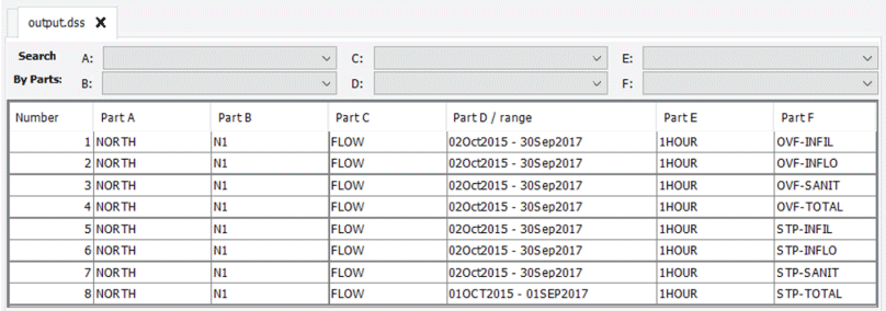
A table with eight entries shows output path parts in Hydrologic Engineering Center-Data
Storage System Visual Utility Engine. — Figure 6.
Example output outflow time series file viewed in Hydrologic Engineering Center-Data Storage System Visual Utility Engine. [OVF, sewer overflow; STP, sewer treatment plant flow; TOTAL, total flow; INFIL, sewer infiltration; INFLO, stormwater flow; SANIT, sanitary flow]

Each time series in the output outflow time series HEC–DSS file contains 1-hour instantaneous runoff data, in cubic feet per second. An example SUBRO time series for the period ranging from October 2, 2015, to September 30, 2017, is shown in figure 7, plotted and tabulated in HEC–DSSVue. The figure also shows the same data for a 24-hour period to provide a clearer depiction of the constituent and total flows.

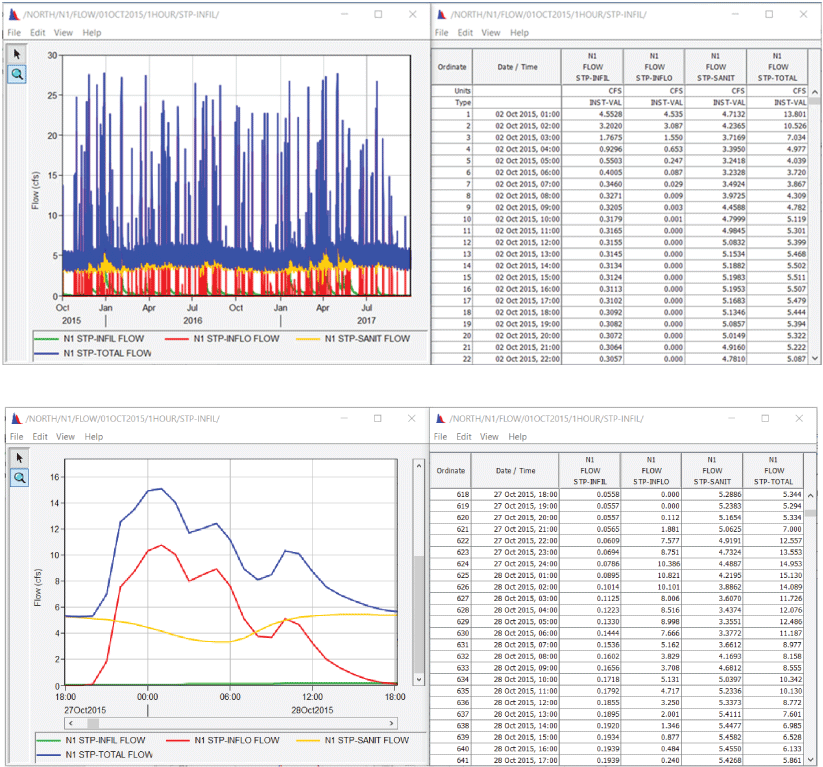
Time series plots and tables show sewer outflows over a 2-year period and 24-hour
period in Hydrologic Engineering Center-Data Storage System Visual Utility Engine. — Figure 7.
Example output sewer flow time series plotted and tabulated in Hydrologic Engineering Center-Data Storage System Visual Utility Engine for the period ranging from October 2, 2015, to September 30, 2017 (top), and for a 24-hour period ranging from October 27, 2015, at 1800 hours to October 28, 2015, at 1700 hours (bottom).

Descriptive Text Output

For every SCALP simulation, a descriptive output log is generated and saved as a text file. This file contains descriptive text, including a copy of the command line arguments and input file as read by SCALP, the land segment input HEC–DSS paths, and the output HEC–DSS paths. An example output text file is shown in its entirety in figure 8A and B; comment lines in the input file, which begin with “+++,” are ignored by SCALP and do not appear in the output text file. In figure 8A and B, spaces are represented by a middle dot character.

A total of 132 lines show text outputs. — Figure 8.
Example output text files. A, part one, showing the command line arguments and input file as parsed by Special Contributing Area Loading Program; B, part two, showing the input and output Hydrologic Engineering Center-Data Storage System paths. Spaces are represented by a middle dot character.

Figure 8.
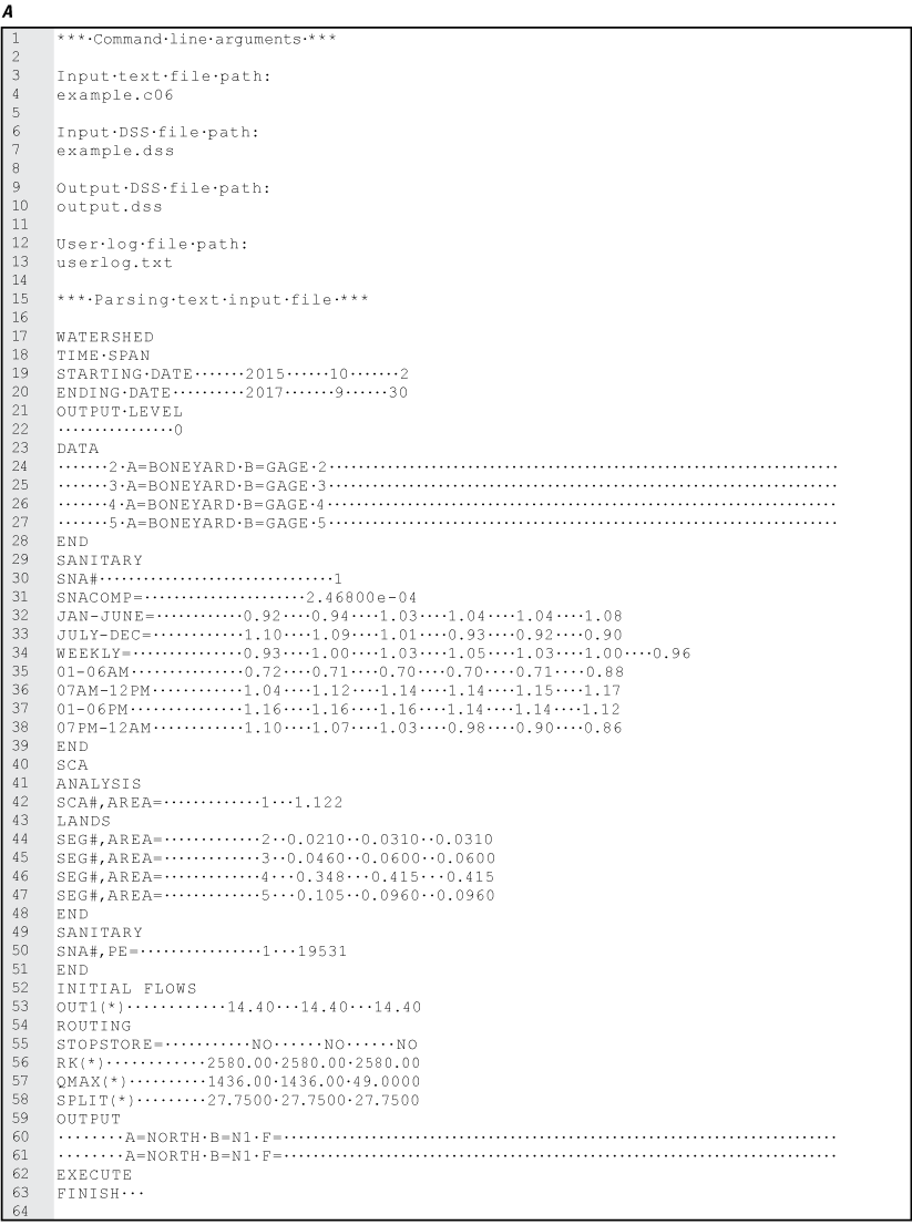
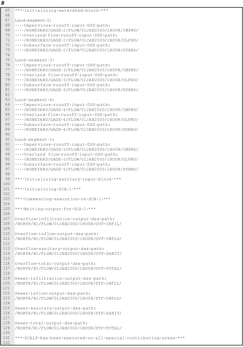
Example output text files. A, part one, showing the command line arguments and input file as parsed by Special Contributing Area Loading Program; B, part two, showing the input and output Hydrologic Engineering Center-Data Storage System paths. Spaces are represented by a middle dot character.

Summary

The Special Contributing Area Loading Program (SCALP) is a hydrologic routing program that simulates reservoir routing through a linear-reservoir-in-series method. SCALP models flow through three reservoirs in series using an input runoff depth time series and information describing the hydrologic characteristics and sanitary flow for one or more land areas within a basin, supplied by the user. To run a successful SCALP simulation on one or more Special Contributing Areas, the user must supply a hydrologic time series and descriptive text file pertaining to each Special Contributing Area, in the formats detailed in this report. Upon completion of a successful SCALP simulation, the program outputs hydrologic time series and a descriptive text file containing the model results. The output time series contain flows through and overflows from the three reservoirs in the series, and the text file contains input and output path locations.

References Cited

Chow, V.T., Maidment, D.R., and Mays, L.W., 1988, Applied hydrology: New York, McGraw-Hill, 572 p.

Domanski, M.M., and Doyle, H.F., 2023, SCALP (Special Contributing Area Loading Program, ver. 1.0.0): U.S. Geological Survey software release, accessed December 8, 2023, at https://doi.org/10.5066/P9EE0614.

Euler, L., 1768, Institutionum calculi integralis volumen primum: St. Petersburg, Imperial Academy of Sciences, v. 1, 542 p.

Kutta, W., 1901, Beitrag zur näherungsweisen Integration totaler Differentialgleichungen: Leipzig, Zeitschrift für Mathematik und Physik, v. 46, p. 435–453.

Pedersen, J.T., Peters, J.C., and Helweg, O.J., 1980, Hydrographs by single linear reservoir model: American Society of Civil Engineers, Journal of Hydraulics Division, v. 106, no. HY5, Proc. Paper 15430, p. 837–852.

Runge, C.D.T., 1895, Ueber die numerische Auflösung von Differentialgleichungen: Mathematische Annalen, v. 46, no. 2, p. 167–178. [Also available at https://doi.org/10.1007/BF01446807.]

Conversion Factors

U.S. customary units to International System of Units


Multiply	By	To obtain
Length
inch (in.)	2.54	centimeter (cm)
inch (in.)	25.4	millimeter (mm)
Area
square mile (mi²)	259.0	hectare (ha)
square mile (mi²)	2.590	square kilometer (km²)
Volume
cubic foot (ft³)	28.32	cubic decimeter (dm³)
cubic foot (ft³)	0.02832	cubic meter (m³)
Flow rate
cubic foot per second (ft³/s)	0.02832	cubic meter per second (m³/s)
inch per hour (in/h)	0.0254	meter per hour (m/h)

Abbreviations

HEC–DSS: Hydrologic Engineering Center-Data Storage System
HEC–DSSVue: Hydrologic Engineering Center-Data Storage System Visual Utility Engine
IMPRO: impervious runoff
ODE: ordinary differential equation
OLFRO: overland flow runoff
RK4: fourth-order Runge-Kutta
SCA: Special Contributing Area
SCALP: Special Contributing Area Loading Program
SUBRO: subsurface runoff

For more information about this publication, contact:

Director, USGS Central Midwest Water Science Center

405 North Goodwin

Urbana, IL 61801

217–328–8747

For additional information, visit: https://www.usgs.gov/centers/cm-water

Publishing support provided by the

Rolla Publishing Service Center

Suggested Citation

Doyle, H.F., and Domanski, M.M., 2024, Special Contributing Area Loading Program user’s manual: U.S. Geological Survey Open-File Report 2024–1021, 15 p., https://doi.org/10.3133/ofr20241021.

ISSN: 2331-1258 (online)

Additional publication details
Publication type	Report
Publication Subtype	USGS Numbered Series
Title	Special Contributing Area Loading Program user’s manual
Series title	Open-File Report
Series number	2024-1021
DOI	10.3133/ofr20241021
Year Published	2024
Language	English
Publisher	U.S. Geological Survey
Publisher location	Reston, VA
Contributing office(s)	Central Midwest Water Science Center
Description	Report: vi, 15 p.; Software Release
Online Only (Y/N)	Y
Additional Online Files (Y/N)	N
Google Analytic Metrics	Metrics page

Special Contributing Area Loading Program User’s Manual

Table of Contents

Links

Acknowledgments

Introduction

(1)

(2)

(3)

Reservoir Routing

Linear Reservoir

(4)

(5)

(6)

Integration Methods

(7)

(8)

(9)

Usage

Installation

Hydrologic Time Series Input

Special Contributing Area Inputs

Table 1.

Watershed Input Block

Table 2.

Sanitary Input Block

Table 3.

Special Contributing Area Input Block

Table 4.

Model Results

Hydrologic Time Series Output

Descriptive Text Output

Summary

References Cited

Conversion Factors

Abbreviations

For more information about this publication, contact:

Suggested Citation