

Joint Agency Commercial Imagery Evaluation (JACIE) Best Practices for Remote Sensing System Evaluation and Reporting
Links
- Document: Report (2.2 MB pdf) , HTML , XML
- Download citation as: RIS | Dublin Core
Executive Summary
The Joint Agency Commercial Imagery Evaluation (JACIE) partnership consists of six agencies representing the U.S. Government’s commitment to promoting the use of high-quality remotely sensed data to meet scientific and other Federal needs. These agencies are large consumers of remotely sensed data and bring extensive experience in the assessment and use of these data. The six agencies are as follows:
-
• National Aeronautics and Space Administration
-
• National Geospatial-Intelligence Agency
-
• National Oceanic and Atmospheric Administration
-
• U.S. Department of Agriculture
-
• U.S. Geological Survey
-
• National Reconnaissance Office
JACIE was formed in 2001 to assess the quality of data from the nascent commercial high-resolution satellite industry. Since then, JACIE has expanded its purview to include data at various resolutions, including commercial and civil.
The processes and techniques used by the JACIE agencies to assess data quality have been compiled within this report to share them across the agencies and with others who want to assess remotely sensed imagery data or understand how data are assessed and reported by JACIE.
Introduction
This document provides an overview of best practices and suggested metrics for reporting system specifications and measured qualities of remotely sensed data, which includes measurements gathered prior to launch and during operational imaging. These assessment and reporting practices help users understand the quality and potential for data, as well as make comparisons among different data.
Overview
The best practices outlined in this report have been derived from industry approved Joint Agency Commercial Imagery Evaluation (JACIE) processes and procedures. JACIE was formed to leverage resources from several Federal agencies for the characterization of remote sensing data and to share those results across the remote sensing community. More information about JACIE is available at https://www.usgs.gov/calval/jacie.
Background
Joint Agency Commercial Imagery Evaluation History
The Joint Agency Commercial Imagery Evaluation (JACIE) partnership was established in 2001 to better understand the characterization and calibration of space-borne remote sensing. JACIE member agencies include the National Aeronautics and Space Administration (NASA), National Geospatial-Intelligence Agency, National Oceanic and Atmospheric Administration (NOAA), U.S. Department of Agriculture, National Reconnaissance Office, and U.S. Geological Survey (USGS).
JACIE represents the U.S. Government’s commitment to using remote sensing technology to provide information for critical science needs and other applications. The USGS website for JACIE includes information on past, current, and future JACIE efforts and can be accessed at https://www.usgs.gov/calval/jacie.
JACIE fulfills its mission through a unique interagency team of scientists and engineers who evaluate the quality and utility of commercial and civil government remote sensing data. JACIE’s role has evolved in response to changes in technologies, methods, and needs. As a result, team members define metrics, prioritize requirements, and assess and assign quality measures for image datasets acquired by the U.S. Government.
In addition, extended relationships are established via JACIE that span civil and military organizations and include national and international government, academia, and industry. The acronym JACIE can refer specifically to the Government partnerships or it can refer to these extended relationships. The acronym JACIE used in the remainder of this document is the latter.
JACIE sponsors an annual workshop to exchange information on the characterization and application of commercial and civil government imagery to all resolutions used by the Government. The event is a face-to-face opportunity for exchanging information.
This report describes common methods JACIE members use to assess data quality. It serves as a model for documenting best practices for how the Government can characterize and assess the quality of remote sensing datasets acquired in support of its needs.
Importance of Data Quality
The importance of calibration and validation of space and aerial remote sensing systems lies in ensuring the quality and integrity of the acquired data and derived products. Methods of calibration and validation are well-documented as a requirement for data acquisition by government and industry. Sensors must be calibrated to provide measurements with the accuracy and precision to meet scientific and other needs.
In the remote sensing world, this need of calibration continues to grow. The calibration of analog film cameras and the resulting “Camera Calibration Report” (Boland and others, 2000) has been known as a requirement for any mapping, engineering, and science work based on the photography acquired by these cameras. From the 1950s until 2019, the National Bureau of Standards, followed by the USGS, operated and provided calibration services and issued these standard reports for the United States and other countries. Although providing a laboratory calibration service for satellites is not feasible, a similar means of ensuring data quality is needed for Earth observation (EO) data from orbit. This need is increased by the speed at which remote sensing, as a technology as well as a practice, is advancing. More data and data products are being produced because it has become easier to build and operate EO satellites, as well as produce data products and perform large-scale analyses.
This data proliferation is spurred by the convergence of technological and economic factors, which include lower cost launch vehicles, higher speed data downloads, high-speed processing at low cost, practically unlimited data storage and archiving capacities, and ease of access to acquire data. These changes are best represented by two substantial outcomes: (1) the rise of low-priced and prolific small satellites (also known as “smallsats”) providing high-resolution and around-the-clock remote sensing data, and (2) the emergence of commercial remote sensing satellite corporations that operate these satellites and provide the data to Government users. The importance of JACIE and a better understanding of remote sensing systems is driven by the sheer number of remote sensing systems, amount of associated data, development of interoperable/integrated products, and many enhanced science-use opportunities.
To enable the use of datasets offered by the growing number of commercial and civil data providers, the products of sensing systems must be calibrated and validated, and their measurement accuracy must be characterized and documented. Such documentation is a critical first step in ensuring products meet user requirements of acceptable data quality. The need and ability to establish a remote sensing baseline that provides calibration to international reference standards, information documentation and continuity, and product validation and monitoring is common for all remote sensing systems. However, the key steps necessary for science quality use are not performed for many sensors because of a lack of knowledge about what is needed and (or) the associated cost.
The push to combine remote sensing inputs to support science has been happening for many years. That effort is now combined with an information revolution that enhances the ability to store, access, and evaluate metadata; and import, use, or create near-real time processing algorithms and high-speed processing. The result is that needed science information can be integrated with the appropriate accuracy and uncertainty levels to meet fit-for-purpose science usability requirements. This push drives the need for JACIE’s best practices report and for their continued enhancement to provide uncertainty information in support of information interoperability.
This document is informed by many years of knowledge from Government civil systems, including Landsat and the Moderate Resolution Imaging Spectroradiometer (MODIS), and their quality baselines and processes. Subsequent sections provide processes to utilize and compare with these well-calibrated reference systems and international standards, as well as provide a reference to enhance data and product quality with an eventual goal of establishing interoperability quality levels for various data streams to meet higher level science product development and application use.
Purpose and Scope
The purpose of this report is to facilitate a common foundational understanding of image data and data product quality for Government and industry through JACIE best practices, which can enable a common approach for the evaluation of image data and data products. The overarching goal is to provide guidance for current (2024) and new remote sensing data providers to demonstrate data quality in accordance with performance and accuracy standards established by JACIE stakeholders. Performance and accuracy standards are affected to a large extent by downstream analysis and relevant applications.
Assessing and understanding the quality of remote sensing data and acquired datasets is crucial for use and decision-making by the Federal Government, including operational production, and scientific research and analysis. Ensuring the acquisition and delivery of quality remote sensing data in support of these domains requires clear and credible documentation of calibration and validation of the sensing systems.
Pre- and Post-Launch Testing and Reporting
Pre-Launch Calibration
Although JACIE efforts focus primarily on data products delivered from orbit, due diligence in the pre-launch testing and characterization of system and sensor performance is critical to generating high-quality EO data from orbit. Even though JACIE is concerned with nonorbit remote sensors and has the same requirement for detailed measures and understanding of the systems internal quality and capability, the on-orbit sensors are only afforded this opportunity at one time: prior to launch. This section expounds on these critical initial efforts and is largely taken from an authoritative reference to pre-launch calibration: “Guidelines for Pre-Launch Characterization and Calibration of Instruments” from the National Institute of Standards and Technology (NIST) (Datla and others, 2011). Please refer to this referenced NIST document for a complete treatment of pre-launch calibration.
Modern sensing systems have attained a high level of sophistication and go through stringent design reviews and fabrication testing to ensure operational functionality. In addition, these systems are calibrated prior to launch for use in the laboratory or designed for field environments to certify adherence to design specifications and performance standards.
As a best practice, prelaunch calibration uncertainties need to be carefully evaluated and tabulated component by component, and the total uncertainty budget is to be made transparent for critical analysis independent from the satellite operator. The analysis covers random and systematic uncertainties. The random type is the uncertainty in the repeatability of measurements. In general, because of good environmental control on the instrumentation and computer acquisition and analysis of the data at a fast rate, the random uncertainties can be made very small in the pre-launch phase. However, these uncertainties need to be recharacterized postlaunch and periodically reassessed on-orbit using a space view of the sensor. While on-orbit, repeatability may be good within a short measurement time interval. In long time-series measurements, however, the sensor may have a drift owing to its degradation in the space environment.
This degradation in instrument performance is a systematic effect that could be corrected if it could be measured or scientifically estimated based on sound error modeling. The systematic effect or its correction will have an uncertainty that can be modeled and quantified. The systematic uncertainties evaluated in the characterization of various parts of the sensor system are also to be evaluated in the pre-launch and post-launch mission phases. The square root of the sum of the squares of these two types of uncertainties gives the combined standard and expanded uncertainty. In addition to measuring these uncertainties, best practice includes providing the accuracy and stability measurements based on repeated on-orbit measurements and compared against the pre-launch design specification.
Stability of the sensor is the ability of the sensor to maintain its repeatability during a time period. Stability is measured by the maximum drift of the short-term average measured value of a variable after appropriate corrections through on-orbit calibrations under identical conditions throughout a decade. The accuracy is a measure of the closeness of the result of measurement and the true value, and is measured as the standard uncertainty of the combined result of all measurements. Both these quantities are prone to both types of uncertainties. In practice, the expanded uncertainties are to be used with appropriate coverage factors to define the interval for expressing the level of confidence for the measured value. Based on NIST recommended best practices, achieving the stability and accuracy requirements for a satellite sensing system is presented as a three-step process.
Step 1. The first step is to determine the mission and calibration requirements. The mission requirements are determined by the project scientist for the type of measurements to be made. It is ideal to have radiometric experts from National Metrology Institutes (NMIs) such as NIST or other professionals active in the field for International System of Units (SI) calibrations involved in the deliberations on radiometric accuracy requirements and availability of SI standards for calibrations.
If one specific requirement is considered, it would be that accurate measurements of solar irradiance are important to defining climate radiative forcing, and its accuracy requirements are specified in a tabular form. The mission requirements are generally specified at the product level, and the development of instrument design and radiometric models with predictions of uncertainties are left to the contractors who compete to fulfill the requirements of the mission.
For example, examine a sensor specification such as “absolute radiance accuracy less than 5 percent required.” Such a statement without giving a coverage factor will be vague and prone to different interpretations. The choice of the traceable transfer standard will be different for different interpretations of the uncertainty requirement for the sensor. For example, if the required level of confidence is corresponding to the interpretation of coverage factor for the accuracy requirement of 5 percent for pre-launch calibration, the requirement on the choice of the transfer standard is not stringent. There is more flexibility in the distribution of the uncertainty in the error budget for the choice of the transfer standard to satisfy the accuracy requirement.
Step 2. The next step includes component and subsystem characterization and modeling the sensor performance. Characterization involves determining the component and subsystem instrumentation responses for various operating and viewing conditions on-orbit emulated in the laboratory. The sensor performance is modeled based on the sensor measurement equation and describes all the influencing parameters on the sensor responsivity. The influencing parameters are of broadly radiometric, spectral, and spatial categories. The radiometric detector characteristics such as linearity, stability, and cross talk; spectral characteristics such as responsivity, stability, and accuracy; and spatial characteristics such as pointing, spatial and angular responsivity, and so forth, are to be characterized.
If spectral transmission of filters is used, it is important to characterize the filters at operating temperatures. The mirror reflectivity and its angular dependence are also very important to characterize. It is important to perform these characterizations at the environmental conditions, such as temperature and vacuum, as they will be on-orbit. However, cost and schedule would need be evaluated and characterizations would need to be planned to meet the requirements. It is highly recommended to take advantage of NASA or other potential JACIE member capabilities and expertise to obtain critical measurements and gain a high degree of confidence in building the sensor model.
The measurement equation of a sensor measuring radiance in digital units can be written in a simplified equation:
whereDNi,j
is the digital number output by instrument detector i in band j,
G
is the instrument detector plus digitization gain,
Ai,j
is the area of detector i in band j,
Ω
is the instrument acceptance solid angle,
L(λ)
is spectral radiance at the sensor’s aperture,
Δλ
is the bandwidth,
η
is the detector quantum efficiency in electrons per incident photon,
t
is the integration time, and
τ
is the instrument optical transmission.
Instrument response nonlinearity, background, focal plane temperature effects, and response versus scan angle effects are not shown in equation 1. These quantities are determined in pre-launch instrument characterization tests and are incorporated in instrument radiometric models and in the production of measured radiances.
Equation 1 can be rewritten as the following:
whereL(λ)
is spectral radiance at the sensor’s aperture,
DNi,j
is the digital number output by instrument detector i in band j, and
m
is outlined in equation 3.
Step 3. To compare model predictions and validate system-level calibration measurements, m is determined pre-launch for an end-to-end remote sensing instrument by viewing uniform sources of known radiance, such as well-characterized and calibrated integrating sphere sources and blackbodies. The characterization of integrating spheres and blackbodies using traceable standards has been extensively reported in published interaction between NIST and NASA for many of the Earth observing system instruments including the sea-viewing wide field-of-view sensor (SeaWiFS) and MODIS pre-launch sensor-level calibrations. Such interactions also took place between NIST and NOAA in the past and are documented in Datla and others (2011).
The quantity, m, also can be determined pre-launch through component and subsystem characterization measurements of quantities such as mirror reflectance, polarization responsivity, and spectral radiance responsivity. These subsystem-level characterization measurements are used as input to instrument radiometric sensor models used to validate the system-level pre-launch calibration and in the calculation of instrument measurement uncertainty as shown as the result of the best practice.
The quantity, m, in equation 3 is monitored on-orbit using stable, uniform, on-board sources of known radiance. Again, on-board blackbody sources or artifacts such as solar diffusers for bidirectional reflectance distribution function (BRDF) measurements are to be developed and characterized as SI traceable standards using the expertise at NMIs such as NIST, as identified in figure 1 and in steps 2 and 3, which are further elaborated in the “Pre-Launch Preparation for Post-Launch Sensor Performance Assessments” section.
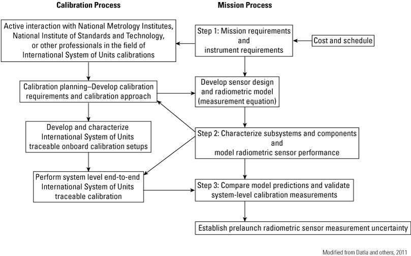
Pre-launch calibration workflow (Modified from Datla and others, 2011).
Pre-Launch Preparation for Post-Launch Sensor Performance Assessments
Preparation for post-launch assessments of measurements and uncertainties is part of the best practice that is to be simultaneously undertaken during pre-launch preparations. An important aspect of pre-launch testing is determining how to prove instrument stability under on-orbit conditions. Stability is often specified for long periods such as mission lifetimes, but it is not possible to test for that long of a period. Thus, a “minimally acceptable” criterion is recommended to be developed during calibration planning and sufficient time would need to be allocated for this pre-launch activity to take place during the final phase of system-level end-to-end calibration.
Plan for Component Performance Reassessments
One of the lessons learned at NIST in previous interactions with NASA and NOAA is that some of the sensor data problems on-orbit could not be isolated fully because no duplicates or even samples of components were available for re-examination. Duplicates of filters, apertures, mirror samples, diffusers, and so forth, are valuable to have for re-examination at metrology laboratories where high-accuracy data can be obtained by simulating on-orbit conditions to sort out data discrepancies.
For example, the band edge wavelength of filter transmission is temperature-dependent and it could be re-measured to understand on-orbit data. At NOAA, in the case of Geostationary Operational Environmental Satellite (GOES) sounder on GOES–N and high-resolution infrared sounder on polar operational environmental satellites, a large discrepancy—as high as 6 degrees Kelvin—was observed between the measured radiance of an on-orbit blackbody and that radiance calculated using the pre-launch vendor-supplied spectral response function (SRF) of the sensor. This discrepancy affected the on-orbit product retrieval and assimilation of numerical weather prediction models because the atmospheric quantity of interest is determined by varying it to make calculated radiances match with observed atmospheric radiances.
The calculated radiance is essentially a convolution of the SRF with the monochromatic radiances from radiative transfer computation. Therefore, as a first step, NOAA employed NIST to make independent measurements of SRFs of witness samples of filters of on-orbit GOES sounders. In the affected channels of GOES–8 and GOES–10 sounders, NIST measurements done at the on-orbit operational temperature conditions disagreed with SRFs in use by NOAA and were determined to be more consistent with on-orbit radiance observations at known blackbody temperatures, thus explaining the possible discrepancy (American Society for Photogrammetry and Remote Sensing, 2014).
A similar investigation was completed on high-resolution infrared sounder filters to compare vendor measurements and NIST measurements (Cao and Ciren, 2004). Again, there were noticeable discrepancies, and the NOAA analysis showed such discrepancies affect product retrievals and their inferences on weather prediction models. As a lesson learned from this interaction, it is essential to have SRFs measured at simulated on-orbit operating conditions and they should be independently verified with authentic witness samples.
One simple best practice based on lessons learned in NASA missions is that each satellite mission should have duplicates of critical components of their radiometric instruments for future on-orbit data reassessments. Furthermore, this best practice guideline could be extended to the manufacture of key instrument subsystems within specific filters and to have instrument representatives in the manufacturing facility to monitor component testing and acquire authentic duplicates of space hardware.
Post-Launch and Pre-Launch Validation and Traceability
Post-launch. Part of the overarching principles advocated by the workshop report (Datla and others, 2011) for high-quality climate observations is to arrange for production and analysis of each climate data record independently by at least two sources. It goes on to state, “Not only instruments, but also analysis algorithms and code require validation and independent confirmation” (Datla and others, 2011, p. 630). This requirement is because confidence in the quantitative value of a geophysical parameter will be achieved only when different systems and different techniques produce the same value (within their combined measurement uncertainties). Comparisons of the results by different sources are expected to reveal the origin of the flaw to be corrected by their advocates to improve the confidence of their systems and techniques to produce high-quality data.
This process is broadly called “validation” and is defined by the Working Group on Calibration and Validation (WGCV) of the Committee on Earth Observation Satellites (CEOS). Traditionally the process is completed post-launch through ground “truth” campaigns where different satellite systems compare their measurements on ground “truth” sites. This validation process requires that the ground “truth” system has proved capable of credible datasets. Post-launch validation should be planned using land sites of known radiometric characterization.
For instruments such as the Advanced Very High-Resolution Radiometer, the ground “truth” sites essentially provide what is called “vicarious calibration.” For satellite sensors such as SeaWiFS, the instrument calibration that began in the laboratory is continuing through vicarious calibration by comparison of data retrievals to in-water, ship, and airborne sensors to adjust instrument gains. The WGCV of CEOS is identifying suitable sites and their characteristics for on-orbit sensor validations and vicarious calibrations for sensors worldwide (Committee on Earth Observation Satellites, undated). CEOS WGCV members are working with NMIs such as NIST in the United States and the National Physical Laboratory in the United Kingdom in this effort. One site selected is the moon, as an on-orbit stability monitor for the visible and near infrared spectral region up to 2.5 micrometers. The SeaWiFS and MODIS sensors currently on-orbit have been successfully viewing the moon as a stability monitor. One of the recommendations of the Achieving Satellite Instrument Calibration for Climate Change workshop is that necessary lunar observations be carried out to make the moon an SI traceable absolute source for on-orbit satellite calibrations.
Programs at NASA and NOAA provide high-altitude aerial platforms with radiometrically calibrated sensors for validation of satellite sensor data by simultaneously observing the satellite sensor footprint of Earth’s atmosphere (for example, the University of Wisconsin Scanning Hyperspectral Imaging Spectrometer; Federal Geographic Data Committee, 1998).
Pre-launch. In following the various steps of best practice in figure 1, new research methods and other advancements in technology can be investigated to help improve the uncertainties.
Although not yet proven for satellite sensor pre-launch validation activity, it is becoming possible in the laboratory to project special scenes that are radiometrically calibrated, which is achieved by using a light source and a digital micromirror device to project a scene of interest (Datla and others, 2011). The spectral engine and the spatial engine are two digital micromirror device projectors independently illuminated by light sources and controlled to project the appropriate combination of the spectral features and the spatial features. Algorithms are used to develop appropriate combination of basis spectra to project the real scene of interest.
High-quality image data could be projected to the sensor, and thus preflight validation could be emulated with on-orbit sensor data samples. As the accuracy of this validation equipment improves, such an exercise could help evaluate the sensor performance more realistically.
On-Orbit Intercomparisons and International System of Units Traceability
It is best to have intercomparisons of similar sensors on-orbit to assess consistency in data products and sensor performance. Such intercomparisons are possible when both sensors being intercompared are SI traceable on-orbit. Intercomparison of on-orbit sensors has become possible with the technique of simultaneous nadir overpass (SNO) (Gil and others, 2020): when both satellites observe the same footprint at nearly the same time, they cross each other in their orbits.
To bring self-consistency and intercalibration among sensors, a group called Global Space-based Inter-Calibration System formed and is actively pursuing SI traceability for intercalibrations working with NMIs such as NIST. Intercomparisons can find agreement or disagreement between sensors in their radiance measurements. In either case, lessons may be learned on possible systematic effects that are currently ignored or neglected. Because the true value of the measurement on-orbit will always be an unknown quantity, the accuracy of the measurement can best be assessed by combining the results from different sensors and calculating the uncertainty of that combined reference value based on the individual sensor data. The combined reference value and the estimate of its uncertainty in the time series would allow scientists to investigate methods to minimize uncertainty.
On-Board Calibration
The relation between the sensed values and the radiances can be derived by comparison of the sensor signal with an on-board reference. The reference can be the sun, moon, or other constant target. On-board sensor calibration is therefore the basis of reliable remote sensing and ensuring the quality of the derived variables and products; however, post-launch comparison with reference standards of known accuracy is complex. On-board calibration units being interpreted as the reference standard also are subject to degradation processes, especially in the visible spectral range.
Vicarious Calibration
The reflectance/radiance-based method is one of the most common vicarious calibration techniques. This method predicts at sensor (top of atmosphere [TOA]) reflectance or radiance over a selected ground target. This method depends on in situ measurements that accurately characterize the surface and atmosphere during the sensor overpass at the selected test site. These surface and atmospheric measurements are used as an input to a radiative transfer code such as Second Simulation of the Satellite Signal in the Solar Spectrum and Moderate Resolution Atmospheric Transmission. The output of the radiative transfer code is TOA reflectance/radiance, which is compared with the sensor Digital Number, obtained from the image of the selected test site, to give a calibration coefficient. This method also provides an independent assessment of remote sensing data, so it has been widely used to validate level-1 and level-2 data products (Dinguirard and Slater, 1999; Biggar and others, 2003; Thome and others, 2008; McCorkel and others, 2012). Researchers have used this method to calibrate different optical satellite sensors such as EO–1 Hyperion (Biggar and others, 2003; Thome and others, 2008; McCorkel and others, 2012; Jing and others, 2019), Geostationary Operational Environmental Satellite R (GOES–R; McCorkel and others, 2020), and Landsat 8 Operational Land Imager (OLI) level-1 and level-2 data products (Teixeira Pinto and others, 2020).
To automate this process, CEOS WGCV and the Infrared Visible Optical Sensors established the Radiometric Calibration Network (https://www.radcalnet.org/). Currently, the Radiometric Calibration Network contains five radiometric calibration instrumented sites in the United States, France, China, and Namibia. These instrumented sites provide automatic measurement of surface reflectance and atmospheric measurements acquired every 30 minutes between 09:00 and 15:00 local time. These measurements are sourced as input to a radiative transfer model that predicts the corresponding nadir-view TOA reflectance, which is compared with satellite sensor observations to perform its radiometric assessment (Bouvet and others, 2019). Researchers have used this system to perform a radiometric assessment of different optical satellite sensors such as Landsat 8 Operational Land Imager OLI (Markham and others, 2014), Sentinel 2A multispectral instrument imagery, and visible infrared imaging radiometer suite (Czapla-Myers and others, 2017; Barsi and others, 2018).
Qualities—Measuring and Reporting
The importance of defining a framework for the measurement and reporting of satellite data is not to be underestimated. This starts with having a thorough understanding of the operational capabilities of a system, and the data that it produces. Users need to be informed about what to expect in terms of data quality, and the usability, accessibility, and availability of data.
Community undertakings such as Quality Assurance Framework for Earth Observation (QA4EO) are leading the way in defining frameworks that can help provide generally accepted guidelines to measuring and reporting satellite data.
General System Qualities and Specifications
Basic Satellite Specifications and Operating Information
Basic information about a remote sensing satellite provides an essential understanding of the system’s capabilities and expected performance. This information provides the general operating capabilities of a system and the data it generates.
During development, this basic information is often referred to as the system specifications, or the intended operational capabilities of a system. Following launch and the commencement of operations, these specifications should be updated by actual performance specifications. It is important that planned performance is updated with actual on-orbit performance because these are the performance specifications of the system that develop the remotely sensed measurements provided to users.
Basic System Specifications
A description of the core systems specifications, as well as the expected measurement units, are described in tables 1 and 2.
Table 1.
Satellite system specifications.Table 2.
Core systems specifications for imaging sensors.| Basic sensor optical design | Whiskbroom, pushbroom, framing sensor or other |
|---|---|
| Ground sample distance (GSD) | Instrument field of view of each detector at nadir. Note: For very wide-swath instruments, report the GSD at nadir and at the swath edges (meters). |
| Swath width | Width of the imaging swath at nadir; if a sensor is designed to not operate at nadir, a qualifying description should be given (kilometers) |
| Spectral bands | Bandwidth and band center wavelengths reported (or lower-center-upper) for each panchromatic,
multi-, and super-spectral imaging satellites (microns/micrometers) Full spectral characterization of each band is described by the relative spectral response (refer to appendix 3 for an example). |
| Number of bands between lower and upper wavelength for hyperspectral systems that use grating, wedge, or similar methods of dividing a region of the spectrum into many similar-width bands (microns/micrometers). | |
| Radiometric resolution | Number of bits used to quantify the detector response, also known as the bit depth (bits) |
| Product levels offered | Levels of products offered, along with a brief description of each (for example, Level-0, Level-1, …,) |
Geometric/Geodetic Quality
Geometric quality assessment of a remote sensing product independently assesses the geometric characteristics of the imagery. For a multispectral remote sensing product, the assessment usually involves two kinds of validation:
-
• The internal relative band registration accuracy
-
• The assessment of the external geodetic accuracy of the product
Figure 2 shows an example of a geometric error map and histogram, which is part of the geometric quality assessment.
Internal Relative Band Registration
Internal band registration measures how accurately the various spectral bands are aligned to each other. The band registration assessment is typically accomplished by selecting a reference band and measuring the alignment of other bands to this reference band. Alternately, each band can be registered to every other band, if computationally feasible. The assessment provides a numerical evaluation of the accuracy of the band registration within an image. That action is carried out by using automated cross-correlation techniques between the bands to be assessed.
Automated Grayscale Cross-Correlation
When applying automated cross-correlation during band assessment, the reference image is taken to be the image data from one of the bands in the multispectral image product; the rest of the bands are considered search images. This process is repeated cyclically by considering image data from a different band to be the reference image. In this manner, data from each band are analyzed against data from every other band.
In cases where the bands within an image have different resolutions, the reference or the search image is resampled to match the lowest resolution of the two bands. Typically, cubic convolution resampling method is used to resample the data. The band characterization analysis measures the relative alignment of the bands to each other by fitting the residuals from all the band combinations using a least squares method.
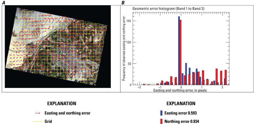
Example of geometric error map and histogram.
Automated Mutual Information-Based Correlation
The mutual information correlation method was developed to register Landsat Enhanced Thematic Mapper Plus (ETM+) scenes affected by the scan-line corrector (SLC) anomaly (Barsi and others, 2016). It is available for use in the Landsat image assessment system (IAS) suite of tools (U.S. Geological Survey, 2006). The correlation process is implemented in a manner similar to the grayscale-based correlation process; however, the matching algorithm uses theoretic means by determining the minima of the joint entropy between two images being registered. Mutual information-based matching is another available option within IAS for measuring band registration. It is, however, more computationally intensive than grayscale correlation.
Manual Tie Points
Manual methods can be used when high-resolution reference and search images are available. In such cases, conjugate points are manually located, and their coordinates are then compared and summarized. The manual methods often rely on the analyst’s knowledge and accuracy in identifying the conjugate points and therefore use of manual methods is recommended to be limited to very high-resolution images. The semi-automated and automated methods can be used for coarse-medium-high resolution images and rely on statistical techniques for error analysis. For accurate results, it is imperative that points be selected from features at ground level.
Ground coordinates of features from the reference image are compared with the corresponding coordinates obtained from the search image. This process measures the relative accuracy of the search image with respect to the reference image. Statistical summaries, such as mean and standard deviation of the residuals from all the conjugate points, provide a measure of the relative geometric offset between the reference and search images. Plotting the points measured between the two images also helps to assess any systematic bias or higher order distortion within the search image.
External Geometry Assessment
External geometry assessment evaluates the absolute positional accuracy of the image products with respect to ground (geometric) reference. The geodetic ground reference is chosen to have known positional accuracy and internal geometric consistencies, which are typically better than the images being evaluated. Measurement and reporting methods are described in the following subsections.
Automated Cross-Correlation
Automated methods, which can be used for coarse to high resolution images, use statistical techniques for error analysis, whereby conjugate points in the reference and search images are identified automatically and refined using similarity measures, such as normalized cross-correlation metrics. Small subimages are then extracted around the conjugate point locations, and image-based correlation methods are used for comparisons.
Ground coordinates of features from the reference image are compared with the corresponding coordinates obtained from the search image. This process measures the relative accuracy of the search image with respect to the reference image. Statistical summaries, such as mean and standard deviation of the residuals from all the conjugate points, provide a measure of the relative geometric offset between the reference and search images. As shown in figure 3, plotting the points measured between the two images also helps to assess any systematic bias or higher order distortion within the search image.
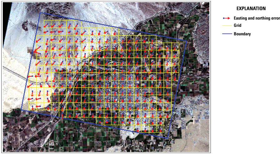
Example of relative geometric error.
Semi-Automated Cross-Correlation
The semi-automated methods, which can be used for coarse-medium-high resolution images, rely on statistical techniques for error analysis. The semi-automated methods follow the same process as the automated methods, except the analyst provides the initial approximation of the conjugate points. Often, the semi-automated methods are used for images that are likely to exhibit high false matches, such as desert, cultivated areas, and urban terrain. In such terrain, automated methods can choose points that may lie on rooftops, which are not acceptable locations (owing to building lean, and so forth). Therefore, the user manually chooses locations for comparisons between reference and search images, ensuring that these locations are on the ground (for example, the corner of a building where it intersects the ground), and in a reasonably uniform distribution.
Ground coordinates of features from the reference image are compared to the corresponding coordinates obtained from the search image. This process measures the relative accuracy of the search image with respect to the reference image. Statistical summaries, such as mean and standard deviation of the residuals from all the conjugate points, provide a measure of the relative geometric offset between the reference and search images. Plotting the points measured between the two images also helps to assess any systematic bias or higher order distortion within the search image.
Geometric Accuracy Reporting Practices
There are many reporting methods for geometric data quality. According to the Federal Geographic Data Committee (FGDC), reporting should indicate the characteristics listed in table 3.
Table 3.
Geometric accuracy reporting characteristics.[%, percent; CE90, 90-percent circular error]
The American Society for Photogrammetry and Remote Sensing has built on FGDC reporting standards (Federal Geographic Data Committee, 2010) to introduce geometric reporting standards (American Society for Photogrammetry and Remote Sensing, 2014). These standards tend to be used by the mapping industry, but the methods remain generic and applicable to JACIE reporting practices as well.
The FGDC developed and approved the National Standards for Spatial Data Accuracy (NSSDA) in 1998. The NSSDA describes a way to measure and report positional accuracy of features in a geographic dataset. Generally, the following steps are taken while evaluating a geographic dataset based on the NSSDA (Federal Geographic Data Committee, 1998) and are detailed in Bruegge and others (1999):
-
• Select independent dataset of higher accuracy (reference data). The American Society for Photogrammetry and Remote Sensing suggests that the accuracy of the reference data be three times the accuracy of the data being studied.
-
• Select test features in the data being evaluated; this could be manual or automated.
-
• Collect positional measurements from conjugate features in both (reference and study) datasets.
-
• Calculate accuracy statistic (root mean square error [RMSEr]).
-
• Prepare an accuracy statement using NSSDA statistic.
In general, the USGS Earth Resources Observation and Science Calibration and Validation Center of Excellence (ECCOE) has reported the circular RMSEr statistic, along with mean errors. The NSSDA statistic follows trivially from the RMSEr statistic as a single multiplication factor. A link to sample worksheets to perform these calculations for three-dimensional data is provided in appendix 1. For image data assessment that does not include elevation information, the columns regarding elevation or “Z” statistics can be ignored. When evaluating digital elevation models where only the elevation values are of chief concern, the X and Y statistic columns can be ignored. In that case, the NSSDA statistic is different when compared to the horizontal accuracy NSSDA statistic (appendix 1)
Spatial Data Quality
Often, the spatial resolution of remotely sensed imagery is described in terms of pixel spacing or ground sample distance (GSD). Although important, GSD is only one aspect of spatial resolution. The optical detectors may have some amount of “blur,” or lack of sharpness. Spatial characterization provides a quantification of that sharpness/blur. There are multiple methods to measure and report spatial performance. Measurement and reporting methods are described in the following subsections.
It should be noted that signal-to-noise ratio (SNR) also directly affects the perceived sharpness of an image. SNR is described further in the “Signal-to-Noise Ratio” section.
Image sharpness can be defined by either spatial data using physical features (measured as a function of X and Y) or spatial frequency data using Fourier analysis (measured as a function of u and v). When spatial data are used, the assessment is said to be in the spatial domain. When spatial frequency data are used, the assessment is said to be in the frequency domain.
Within the intelligence and defense communities, image spatial quality is often expressed in the form of National Imagery Interpretability Rating Scale, which quantifies the ability of trained imagery analysts to perform selected visual detection and recognition tasks. In recent years, a regression-based model, called the General Image-Quality Equation (Hindsley and Rickard, 2006), has been used to predict the National Imagery Interpretability Rating Scale rating using fundamental image attributes such as GSD, modulation transfer function (MTF), or SNR. Although these image quality ratings are widely used by commercial and defense vendors, JACIE prefers image sharpness measurements reported in one of the five measurements listed in table 4.
Spatial Domain Measures
As mentioned previously, image sharpness can be defined using spatial data. When spatial data are used, the assessment is said to be in the spatial domain. Measurement and reporting methods are described in the following subsections.
Edge Spread Function
Edges are present in many scenes in urban and rural areas and may be used as targets. The spatial quality using edges can be quantified by measuring the rate of transition of intensity across an edge. This can be accomplished by generating the edge spread function (ESF), as shown in figure 4, or by normalized edge response where the intensity has been normalized between 0 and 1. USGS maintains a list of spatial calibration and validation sites at the following location: https://calval.cr.usgs.gov/apps/spatialsites_catalog.
An edge target, which can be automatically or manually selected, is shown in figure 4. The ESF is generated by aligning the transects and normalizing the values to one.
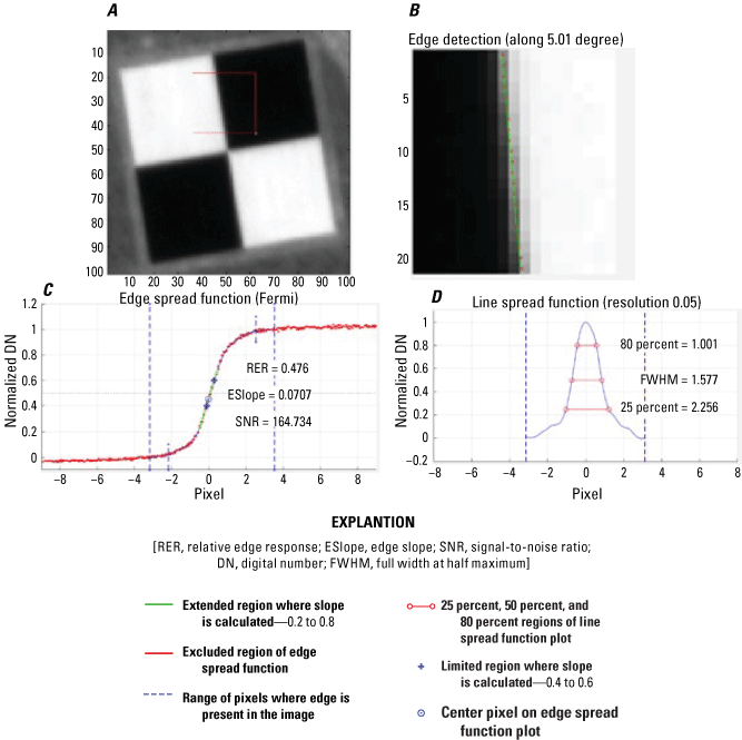
Spatial assessment of edge targets. A, Raw edge transect. B, Edge spread function. C, Line spread function. D, Modulation transfer function.
Ideally, if the goal is to understand the quality of the imaging system, the process should be applied to raw unprocessed images. However, our analysis is done on processed and even resampled products because these products are most preferred by the user community.
-
• Ideally, edges are at least 10 pixels long, although results can sometimes be gathered on edges as small as five pixels in width. The extent of homogenous areas on each side of the edge should also be five or more pixels deep from the edge.
-
• Edges used to measure relative edge response (RER) should be inclined, but not at 45 degrees; vertical or horizontal edges are not useful because they do not provide enough range of edge intersections to create a good understanding of edge response.
-
• MTF targets as shown in table 4, if sufficiently wide, can be used to estimate SNR if their homogeneity is known (refer to “Signal-to-Noise Ratio” section).
Using the normalized edge response, three quantities are further calculated: RER, the full width half maximum (FWHM), and the MTF. The RER is defined as the slope of the ESF between plus or minus 0.5 pixel from the center of the edge. The FWHM is defined from the line spread function (LSF).
Image Quality Estimation Tool
The image quality estimation (IQE) tool (Innovative Imaging and Research, 2018) is a spatial analysis tool that was developed for the USGS under contract. IQE can estimate the spatial resolution performance of an image product by finding, selecting, and using uniform, high-contrast edges that normally occur within many acquired scenes such as field boundaries and straight roads. Large numbers of images containing many edges can be evaluated rapidly by using this tool. By using IQE, benefits include trending analysis of image performance, automated image quality assessment, and quantification of image sharpness parameters.
A graphical user interface is used for IQE to ease use and provide performance consistency. This interface provides an easy-to-understand method to process large quantities of data and to visualize spatial quality summary statistics. Instead of using traditional edge targets, IQE uses features present within aerial and satellite images. Therefore, for the IQE to be successful, the imagery must contain features consistent with the GSD of the imager being assessed. As an example, if Landsat 8 or 9 data (U.S. Geological Survey, 2021) are being processed, features large enough to create a near horizontal or near vertical edge that is approximately 360 meters need to be present in the imagery (at least 12 pixels x 30 meters GSD). For this case, large uniform agricultural fields, such as those frequently found in the midwestern United States, would be appropriate.
Note that the IQE tool requires some inclination to the edges that are used, and that perfectly north to south or east to west edges will not work for analysis.
Line Spread Function
The LSF is the derivative of the ESF, and the width at one-half the maximum value of the LSF is defined as the FWHM. Both RER and FWHM are in the spatial domain and easier to visualize. The MTF measures the spatial quality in the frequency domain and is defined as the Fourier transform of the LSF/point spread function (PSF) (Gaskill, 1978; Boreman, 2001; Goodman, 2005; Holst, 2006). The MTF measures the change in contrast, or modulation, of an optical system’s response at each spatial frequency. The standard MTF measure is the MTF at Nyquist frequency, defined to be the highest spatial frequency that can be imaged without causing aliasing (0.5 cycle per pixel). The SNR is also derived as defined in Helder and Choi (2005).
Point Spread Function
The PSF is a measure of the ability of an imaging system to resolve spatial objects that can be described mathematically by a PSF (Mahanakorn University of Technology, 2017). A point object or an object in space can be imaged using an optical sensor system, which also stores its image. In an ideal system, the point source of light or object should be imaged as a point without any dimensions; however, in the real world, any optical system will capture the image as an unclear circular object of finite dimensions. The PSF is defined by the dimensions of this unclear image. The MTF, which is the magnitude of the Fourier Transform of the PSF, is also used as a measure of the spatial quality of an imaging system.
Radiometric Data Quality
Radiometric data quality measures the accuracy with which the remotely sensed data product reports the radiance or reflectance of the surface contained within a pixel. Measurement methods are described in the following subsections.
Linear Regression
The radiometric characterization requires accurate geometric alignment between two images from different sensors. Usually the georeferencing of different satellite sensors is performed independently; thus, it is not rare for the relative georeferencing error to be substantial. Effectively, the comparison results in the juxtaposition of different pixels, which results in worse than true comparison. Each plot in figure 5 is a scatter plot between two sensors for each band (typical blue, green, red, and near infrared band). For georeferencing to be accurate, a pixel located in a fixed location on the Earth’s surface within one image must match the same pixel in the other image. However, if there is mismatch in georeferencing between two sensors, the scatter plot indicates much wider distribution as shown in figure 5. Accordingly, the regression line is substantially different compared to the geo-corrected scatter plot (fig. 6), which demonstrates the importance of relative georeferencing correction.
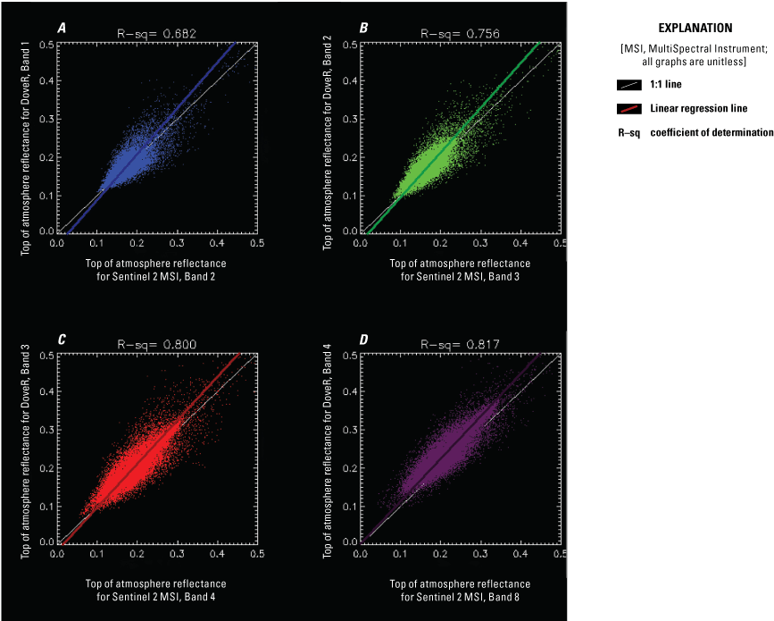
Top of atmosphere reflectance scatter plot and regression without relative georeferencing error correction. A, Dover, band 1; and Sentinel 2 MultiSpectral Instrument (MSI), band 2. B, Dover, band 2; Sentinel 2 MSI, band 3. C, Dover, band 3; Sentinel 2 MSI, band 4. D, Dover, band 4; Sentinel 2 MSI, band 8.
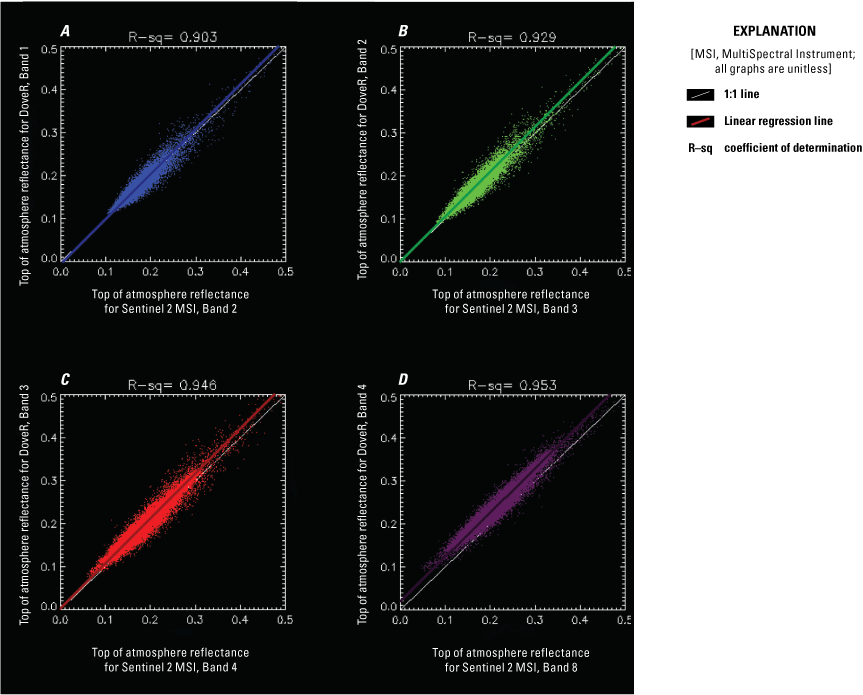
Top of atmosphere reflectance scatter plot and regression after correcting relative georeferencing error. A, Dover, band 1; and Sentinel 2 MultiSpectral Instrument (MSI), band 2. B, Dover, band 2; Sentinel 2 MSI, band 3. C, Dover, band 3; Sentinel 2 MSI, band 4. D, Dover, band 4; Sentinel 2 MSI, band 8.
One of the most common surface types that has been extensively used to perform trending and cross-comparison of satellite sensors is pseudo-invariant calibration sites (PICS) (Helder and others, 2010). PICS are locations on the Earth’s surface that are considered temporally, spatially, and spectrally stable with time. PICS provide a measure of stability or change present in the sensor’s radiometric response and are used for trending of sensor calibration gains and biases with time, sensor cross-calibration, and development of absolute sensor calibration models. The CEOS worked with partners around the world to establish a set of CEOS-endorsed, globally distributed, reference standard PICS for the post-launch calibration of space-based optical imaging sensors. These sites are listed in the USGS calibration and validation test sites catalog (U.S. Geological Survey, 2024b).
Simultaneous Nadir Overpass
Radiometric assessment is usually performed by cross-comparison of images between the sensor to be assessed and the reference sensor, usually Landsat, Sentinel, MODIS, and so forth, using SNO. The SNO calibration technique is a sensor intercalibration method that radiometrically scales the target sensor with the reference sensor using coincident and collocated scene pairs. SNO scene pairs between sensors are used to minimize atmospheric and BRDF effect. SNO-based intercomparison can be done using any surface type but commonly is preferred in a homogeneous area to minimize misregistration error.
Signal-to-Noise Ratio
The measurement of SNR determines how much of the reported radiometric response is from the signal reflected/emitted from the target (signal) and how much is from spurious signals developed within the imager electronics, detectors, compression, transmission, and so forth. Larger SNR values result in clearer imagery. Regardless of the cause of the noise, it affects image radiometric accuracy and, if severe, degrades spatial resolution.
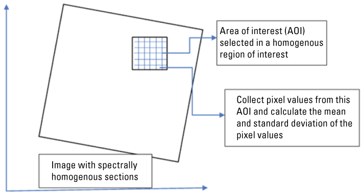
Measuring SNR is difficult unless the base radiance/signal is well known. SNR is often measured at the sensor/detector level. In this document, the SNR is broadly validated using measurements generally over special targets engineered for homogeneity or dark targets, such as the empty ocean at night, that are considered homogenous. An area of interest is identified over such regions, and the mean and standard deviation of the pixel values over this area of interest are determined. The ratio of mean to the standard deviation is used and reported as the SNR. Ideally, this task would be performed and reported for all spectral bands. SNR, as adopted by the USGS ECCOE, is defined in appendix 2.
Radiance/Reflectance
Radiometric correction is a prerequisite for generating high-quality scientific data, making it possible to discriminate between product artifacts and real changes in Earth processes, as well as to accurately produce land cover maps and detect changes. This work contributes to the automatic generation of surface reflectance products for the Landsat satellite series. Surface reflectance products are generated by a new approach developed from a previous simplified radiometric (atmospheric plus topographic) correction model. The proposed model keeps the core of the old model (incidence angles and cast-shadows through a digital elevation model, Earth to Sun distance, and so forth) and adds new characteristics to enhance and automatize ground reflectance retrieval.
Satellite sensor data needs to be converted to physical units such as radiance and reflectance to be useful for the scientific community. The digital numbers recorded by the satellites are converted to at-sensor spectral radiance and TOA reflectance using information usually provided in the metadata files. For the standard radiance products, the calibrated digital numbers often can be converted to at-sensor spectral radiance using the radiometric scale factor, Mλ, and a bias parameter, Aλ (both parameters are usually present in the metadata). The at-sensor spectral radiance is calculated using the following equation:
whereTop of Atmosphere Reflectance
Radiance data conversion to TOA reflectance is the fundamental step in putting image data from multiple sensors and platforms onto a common radiometric scale. A reduction in image-to-image variability can be achieved through normalization for solar irradiance by converting the at-sensor spectral radiance to a planetary or exoatmospheric reflectance. The TOA reflectance of the Earth is computed according to the following equation:
whereLλ
is spectral radiance at the sensor’s aperture;
ρλ
is planetary directional TOA reflectance for Lambertian surfaces, unitless;
d
is Earth to Sun distance, in astronomical units;
ESUNλ
is mean exoatmospheric solar irradiance; and
θs
is solar zenith angle, in degrees.
The TOA reflectance, ρλ, is proportional to the spectral radiance at the sensor’s aperture (Lλ) and the square of the Earth to Sun distance (d) in astronomical units divided by the mean exoatmospheric solar irradiance (ESUNλ) and cosine of the solar zenith angle (θs). The ESUNλ values are dependent on wavelength and solar spectrum model used in the calculation of TOA reflectance.
When comparing images from different sensors, using TOA reflectance instead of at-sensor spectral radiance has three advantages. First, TOA removes the effect of solar zenith angle owing to the time difference between data acquisitions. Second, TOA reflectance compensates for different values of the exoatmospheric solar irradiance arising from spectral band differences. Third, the TOA reflectance corrects for the variation in the Earth to Sun distance between different data acquisition dates. These variations can differ geographically and temporally.
Several factors can be addressed while comparing reflectance from two or more sensors. A consistent solar exoatmospheric model spectrum is vital because different solar exoatmospheric models are slightly different and can increase the discrepancy while comparing reflectance of two sensors. Relative radiometric sensor comparison is performed in the TOA reflectance space to eliminate the differences originated by solar zenith angle and Earth to Sun distance. The atmospheric difference between the acquisitions and the effect of BRDF owing to forward scattering or backscattering would need to be determined, if desired for higher accuracy. A compensation is made for spectral band differences, if required, using the spectral band adjustment factors.
After all conversions and corrections applied to image data from compared sensors, several regions of interest (fig. 7A) are selected from one or more near-simultaneously acquired image pairs. Corresponding regions from the reference and search sensors are usually registered and selected using cross-correlation. Average reflectance values for regions of interest from reference and assessed sensor images are calculated and plotted (as shown in fig. 7B).
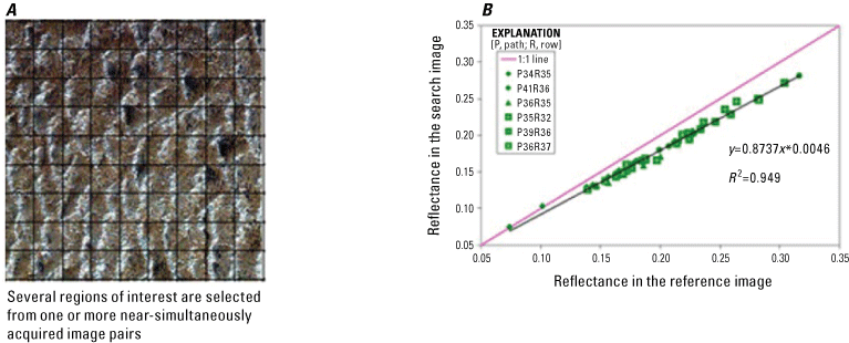
Region of interest sample for Libya 4 pseudo-invariant calibration site (500 x 500 pixels). (Available at https://calval.cr.usgs.gov/apps/libya-4). A, Several regions of interest are selected from one or more near-simultaneously acquired image pairs. B, Reflectance in the search image plotted against Reflectance in the reference image.
In figure 7B, the comparison between reflectance in the search image (Y-axis) and reference image (OLI, X-axis). For a perfectly aligned pair of sensors, the plot should have values as close to the 1:1 line as possible. However, a linear distribution of points indicates that the sensors are aligned in a linear manner, and it is possible to extract the same information from one of the sensors by adjusting the other with the slope from the regression fit. The deviations from the line-fit are possibly a result of differences in the relative spectral response (RSR), sensor characteristics, and so forth.
Artifacts
Artifacts are anomalous features or characteristics within an image that are not present in the target itself. There are many types of artifacts such as missing lines, dropped detectors, saturation, and more. Some known artifacts and how to measure and report them are described in the following subsections.
Systematic, geometric, radiometric, and terrain correction provide the highest quality data to the user communities. Occasionally, system anomalies occur, and artifacts are discovered that require research and monitoring. The system characterization team investigates and tracks anomalous data. This section describes some of these artifacts.
Stray Light
The signal of a given sample is polluted by stray light coming into the instrument from other samples by means of either specular reflections (ghost images) or scatter. Stray light may be a substantial contributor to the measured signal, particularly in the infrared for ocean pixels close to clouds or land covered by vegetation.
The ocean and land color instrument (OLCI) stray light correction algorithm (European Space Agency, 2024a) is defined below. It uses characterization of stray light contamination to estimate the degradation and correct it. Stray light contribution to signal is evaluated from the already contaminated signal on the assumption that because it is a small contribution, the fundamental signal structure is preserved, and it can be considered as Epsilon in the approximation:
Once estimated it can be corrected. A two-step process is used:
-
● A first contamination taking place in the ground imager (that is, the imaging part of the instrument optics) with mixing of energy from the whole field-of-view, including both spatial dimensions, but without spectral mixing.
-
● A second contamination occurring inside the spectrometer, with one spatial dimension (the along-track direction) filtered out by the spectrometer entrance slit but including spectral mixing through scattering and reflections during or after spectral dispersion.
Therefore, stray light correction is implemented in two steps, following the instrument signal generation but in the backward direction. Because the output from radiometric scaling corresponds to the signal sensed at the charge coupled device surface, it includes both stray light contributions. Stray light must therefore be corrected for the spectrometer contribution and then for the ground imager contribution.
The spectrometer stray light term can be expressed as a two-dimensional convolution of the two-dimensional weighted radiance field. Note that the spectral dimension of the charge coupled device is reconstructed from the 21 available samples (the OLCI channels) using linear interpolation on normalized radiance and by avoiding the use of saturated samples.
The ground imager stray light contribution term also can be expressed as a two-dimensional convolution of the incoming radiance field but is expressed independently for each OLCI channel. The stray light contribution term can be estimated from the radiance field corrected for the spectrometer contribution.
Additional Artifacts and Reporting
Additional data artifacts include issues such as dead detectors, detector striping, coherent noise, and data loss. In addition to imagery, artifacts can be found in supporting data, file naming, metadata, and more. As examples, comprehensive lists of known Landsat data and Sentinel-2 data anomalies, along with descriptions of each, can be found in U.S. Geological Survey (2024a) and European Space Agency (2024b), respectively.
If users encounter artifacts when analyzing data, those artifacts should be reported to the system characterization team via the ECCOE web page (https://www.usgs.gov/calval). Depending on the anomaly, corrective measures may be deployable, resulting in higher image data quality. Even if no corrective measures can be utilized, awareness of an artifact will inform the system characterization team of sensor performance issues.
Summary
This report summarizes the best practices that have been derived from industry-approved Joint Agency Commercial Imagery Evaluation (JACIE) processes and procedures. In summary, we have described several processes and procedures that promote a common foundational understanding of image data and data product quality for Government and industry through JACIE best practices, which can enable a common approach for the evaluation of image data and data products. The overarching goal was to provide guidance for current (2024) and new remote sensing data providers to demonstrate data quality in accordance with performance and accuracy standards established by JACIE stakeholders.
In conclusion, the report highlights that the importance of calibration and validation of space and aerial remote sensing systems lies in ensuring the quality and integrity of the acquired data and derived products. Methods of calibration and validation are well-documented as a requirement for data acquisition by Government and industry. The report also summarizes how the Earth Resources Observation and Science Calibration and Validation Center of Excellence (ECCOE) system characterization team typically assesses the data quality of an imaging system by acquiring the data, defining proper testing methodologies, carrying out comparative tests against specific references, recording measurements, completing data analyses, and quantifying sensor performance accordingly. The report also describes common methods JACIE members use to assess data quality and serves as a model for documenting best practices for how the Government can characterize and assess the quality of remote sensing datasets acquired in support of its needs.
The ECCOE project and associated JACIE partners are always interested in reviewing sensor and remote sensing application assessments and would like to collaborate and discuss information on similar data and product assessments and reviews. If you would like to discuss new or alternative methods of system characterization with the U.S. Geological Survey ECCOE and (or) the JACIE team, please email us at eccoe@usgs.gov.
References Cited
American Society for Photogrammetry and Remote Sensing, 2014, ASPRS positional accuracy standards for digital geospatial data: Photogrammetric Engineering and Remote Sensing, v. 81, no. 3, p. A1–A26. [Also available at https://doi.org/10.14358/PERS.81.3.A1-A26.]
Barsi, J.A., Alhammoud, B., Czapla-Myers, J., Gascon, F., Haque, M.O., Kaewmanee, M., Leigh, L., and Markham, B.L., 2018, Sentinel-2A MSI and Landsat-8 OLI radiometric cross comparison over desert sites: European Journal of Remote Sensing, v. 51, no. 1, p. 822–837. [Also available at https://doi.org/10.1080/22797254.2018.1507613.]
Barsi, J.A., Markham, B.L., Czapla-Myers, J.S., Helder, D.L., Hook, S.J., Schott, J.R., and Haque, M.O., 2016, Landsat-7 ETM+ radiometric calibration status: Proceedings of SPIE Optical Engineering and Applications, Volume 9972, Earth Observing Systems XXI. [Also available at https://doi.org/10.1117/12.2238625.]
Biggar, S.F., Thome, K.J., and Wisniewski, W., 2003, Vicarious radiometric calibration of EO-1 sensors by reference to high-reflectance ground targets: IEEE Transactions on Geoscience and Remote Sensing, v. 41, no. 6, p. 1174–1179. [Also available at https://doi.org/10.1109/TGRS.2003.813211.]
Boland, J., Kodak, E., and others, 2000, ASPRS camera calibration panel report: U.S. Geological Survey, Prepared by the ASPRS—The Imaging and Geospatial Information Society, 24 p. [Also available at https://www.asprs.org/a/news/archive/final_report.html.]
Bouvet, M., Thome, K., Berthelot, B., Bialek, A., Czapla-Myers, J., Fox, N.P., Goryl, P., Henry, P., Ma, L., Marcq, S., Meygret, A., Wenny, B.N., and Woolliams, E.R., 2019, RadCalNet—A radiometric calibration network for earth observing imagers operating in the visible to shortwave infrared spectral range: Remote Sensing, v. 11, no. 20, 24 p. [Also available at https://doi.org/10.3390/rs11202401.]
Bruegge, C.J., Chrien, N.L., and Diner, D.J., 1999, (JPL), Level 1 in-flight radiometric calibration and characterization algorithm theoretical basis: Jet Propulsion Laboratory, California Institute of Technology, Earth Observing System Multi-angle Imaging Spectro-Radiometer, 128 p., accessed March 2024 at https://eospso.gsfc.nasa.gov/sites/default/files/atbd/atbd-misr-02.pdf.
Cao, C., and Ciren, P., 2004, In-flight spectral calibration of HIRS using AIRS observations: 6 p. [Also available at https://www.researchgate.net/publication/242158508_IN-FLIGHT_SPECTRAL_CALIBRATION_OF_HIRS_USING_AIRS_OBSERVATIONS.]
Committee on Earth Observation Satellites, undated, MTF reference dataset—Geo-spatial quality reference data set: European Space Agency website, accessed March 2024 at https://calvalportal.ceos.org/nl/mtf-reference-dataset.
Czapla-Myers, J., McCorkel, J., Anderson, N., and Biggar, S., 2017, Earth-observing satellite intercomparison using the radiometric calibration test site at railroad valley: Journal of Applied Remote Sensing, v. 12, no. 1, 10 p. [Also available at https://doi.org/10.1117/1.JRS.12.012004.]
Datla, R.U., Rice, J.P., Lykke, K.R., Johnson, B.C., Butler, J.J., and Xiong, X., 2011, Best practice guidelines for pre-launch characterization and calibration of instruments for passive optical remote sensing: Journal of Research of the National Institute of Standards and Technology, v. 116, no. 2, p. 621–646. [Also available at https://doi.org/10.6028/jres.116.009.]
Dinguirard, M., and Slater, P.N., 1999, Calibration of space-multispectral imaging sensors—A review: Remote Sensing of Environment, v. 68, no. 3, p. 194–205. [Also available at https://doi.org/10.1016/S0034-4257(98)00111-4.]
European Space Agency, 2024a, Stray light correction: Sentinel Online Product Description web page, accessed May 2024 at https://sentinel.esa.int/web/sentinel/technical-guides/sentinel-3-olci/level-1/stray-light-correction.
European Space Agency, 2024b, Sentinel-2 anomaly database: European Space Agency website, accessed March 2024 at https://s2anomalies.acri.fr/.
Federal Geographic Data Committee, 1998, Geospatial positioning accuracy standards, part 3—National Standard for Spatial Data Accuracy: Federal Geographic Data Committee, FGDC-STD-007.3-1998, accessed March 2024 at https://www.fgdc.gov/standards/projects/accuracy/part3/index_html.
Federal Geographic Data Committee, 2010, United States thoroughfare, landmark, and postal address data standard: Federal Geographic Data Committee, FGDC-STD-016-2011, 99 p., accessed March 2024 at https://www.fgdc.gov/standards/projects/address-data/AddressDataStandardPart04.
Gil, J., Rodrigo, J.F., Salvador, P., Gómez, D., Sanz, J., Casanova, J.L., 2020, An empirical radiometric intercomparison methodology based on global simultaneous nadir overpasses applied to Landsat 8 and Sentinel-2: Remote Sensing, v. 12, no. 17, 36 p., accessed March 2024 at https://doi.org/10.3390/rs12172736.
Hindsley, R., and Rickard, L., 2006, The general image quality equation and the structure of the modulation transfer function: Washington, D.C., Naval Research Laboratory, 12 p., accessed March 2024 at https://apps.dtic.mil/sti/pdfs/ADA446848.pdf.
Helder, D., Basnet, B., and Morstad, D.L., 2010, Optimized identification of worldwide radiometric pseudo-invariant calibration sites: Canadian Journal of Remote Sensing, v. 36, no. 5, p. 527–539. [Also available at https://doi.org/10.5589/m10-085.]
Helder, D.L., and Choi, T., 2005, Generic sensor modeling using pulse method: National Aeronautics and Space Administration Technical Reports Server, 58 p., accessed March 2024 at https://ntrs.nasa.gov/archive/nasa/casi.ntrs.nasa.gov/20050214150.pdf.
Imaging and Research, 2018, Image Quality Estimation (IQE) user’s guide: I2R Corp, 8 p., accessed March 2024 at https://www.i2rcorp.com/main-business-lines/sensor-hardware-design-support-services/spatial-resolution-digital-imagery-guideline
Jing, X., Leigh, L., Helder, D., Teixeira Pinto, C., and Aaron, D., 2019, Lifetime absolute calibration of the EO-1 Hyperion sensor and its validation: IEEE Transactions on Geoscience and Remote Sensing, v. 57, no. 11, p. 9466–9475. [Also available at https://doi.org/10.1109/TGRS.2019.2926663.]
Mahanakorn University of Technology, 2017, On-orbit point spread function estimation for THEOS imaging system: Proceedings of Third International Conference on Photonic Solutions, Pattaya, Thailand, 10 p. [Also available at https://doi.org/10.1117/12.2300950.]
Markham, B., Barsi, J., Kvaran, G., Ong, L., Kaita, E., Biggar, S., Czapla-Myers, J., Mishra, N., and Helder, D., 2014, Landsat-8 Operational Land Imager radiometric calibration and stability: Remote Sensing, v. 6, no. 12, p. 12275–12308. [Also available at https://doi.org/10.3390/rs61212275.]
McCorkel, J., Efremova, B., Hair, J., Andrade, M., and Holben, B., 2020, GOES-16 ABI solar reflective channel validation for earth science application: Remote Sensing of Environment, v. 237, 17 p. [Also available at https://doi.org/10.1016/j.rse.2019.111438.]
McCorkel, J., Thome, K., and Ong, L., 2012, Vicarious calibration of EO-1 Hyperion: IEEE Journal of Selected Topics in Applied Earth Observations and Remote Sensing, v. 6, no. 2, p. 400–407. [Also available at https://doi.org/10.1109/JSTARS.2012.2225417.]
Thome, K.J., Arai, K., Tsuchida, S., and Biggar, S.F., 2008, Vicarious calibration of ASTER via the reflectance-based approach: IEEE Transactions on Geoscience and Remote Sensing, v. 46, no. 10, p. 3285–3295. [Also available at https://doi.org/10.1109/TGRS.2008.928730.]
U.S. Geological Survey, 2006, LSDS-54 Landsat 7 (L7) Image Assessment System (IAS) Geometric Algorithm Theoretical Basis Document (ATBD): 181 p. [Also available at https://www.usgs.gov/media/files/landsat-7-image-assessment-system-geometric-atbd.]
U.S. Geological Survey, 2021, LSDS-1747 Landsat 8-9 Calibration and Validation (Cal/Val) Algorithm Description Document (ADD) (ver. 4, January 2021): U.S. Geological Survey, 819 p. [Also available at https://d9-wret.s3.us-west-2.amazonaws.com/assets/palladium/production/s3fs-public/atoms/files/LSDS-1747_Landsat8-9_CalVal_ADD-v4.pdf.]
U.S. Geological Survey, 2024a, Landsat known issues: U.S. Geological Survey web page, accessed March 2024 at https://www.usgs.gov/landsat-missions/landsat-known-issues.
U.S. Geological Survey, 2024b, Test sites catalog: U.S. Geological Survey web page, accessed March 2024 at https://calval.cr.usgs.gov/apps/test_sites_catalog.
References Cited
Federal Geographic Data Committee, 1998, Geospatial positioning accuracy standards, part 3—National Standard for Spatial Data Accuracy: Federal Geographic Data Committee, FGDC-STD-007.3-1998, accessed March 2024 at https://www.fgdc.gov/standards/projects/accuracy/part3.
Minnesota Governor’s Council, 1999, Position accuracy handbook—Using the National Standard for Spatial Data Accuracy to measure and report geographic data quality: Minnesota Governor’s Council, Minnesota Land Management Information Center, 33 p., accessed March 2024 at https://www.mngeo.state.mn.us/committee/standards/positional_accuracy/positional_accuracy_handbook_nssda.pdf.
References Cited
Kim, M., Park, S., Anderson, C., and Stensaas, G.L., 2021, System characterization report on Planet’s Dove Classic, chap. C of Ramaseri Chandra, S.N., comp., System characterization of Earth observation sensors: U.S. Geological Survey Open-File Report 2021–1030, 28 p. [Also available at https://doi.org/10.3133/ofr20211030C.]
Appendix 1. National Standard for Spatial Data Accuracy Worksheet
Appendix 2. Signal-to-Noise Ratio Estimation
µ
is the mean of the homogenous pixels, and
σ
is the standard deviation of pixel values of the homogenous pixels.
Signal-to-noise ratio estimation method.
Appendix 3. Example Spectral Response Curve
-
• The nine spectral bands, including a panchromatic band, are listed below:
-
o Band 1 Visible (0.43–0.45 micrometers [µm]) 30 meters (m)
-
o Band 2 Visible (0.450–0.51 µm) 30 m
-
o Band 3 Visible (0.53–0.59 µm) 30 m
-
o Band 4 Red (0.64–0.67 µm) 30 m
-
o Band 5 Near-Infrared (0.85–0.88 µm) 30 m
-
o Band 6 short-wave infrared (SWIR) 1(1.57–1.65 µm) 30 m
-
o Band 7 SWIR 2 (2.11–2.29 µm) 30 m
-
o Band 8 Panchromatic (0.50–0.68 µm) 15 m
-
o Band 9 Cirrus (1.36–1.38 µm) 30 m
-
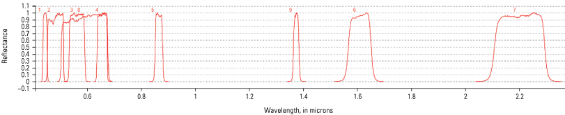
Landsat 8 Operational Land Imager (OLI) spectral response curve.
Appendix 4. Example Geometric Accuracy Report
Table 4.1.
Geometric accuracy report from Planet Dove classic system characterization final report (Kim and others, 2021).[m, meter; SD, standard deviation; RMSE, root mean square error]
Appendix 5. Calibration and Validation Tools
Table 5.1.
Tools used to perform calibration and validation[ENVI/IDL, ENVI’s Interactive Data Language; FLAASH (MODTRAN), ENVI's Atmospheric Correction Module; EROS_SC, Earth Resource Observations and Science – Sensor Characterization tool I2R IQE, Innovative Imaging & Research’ image quality estimation tool]
Appendix 6. How to Obtain Exoatmospheric Spectral Irradiances (ESUN) Values
        <Solar_Irradiance_List>
          <SOLAR_IRRADIANCE bandId=”0” unit=”W/m2/µm”>1884.69</SOLAR_IRRADIANCE>
          <SOLAR_IRRADIANCE bandId=”1” unit=”W/m2/µm”>1959.66</SOLAR_IRRADIANCE>
          <SOLAR_IRRADIANCE bandId=”2” unit=”W/m2/µm”>1823.24</SOLAR_IRRADIANCE>
          <SOLAR_IRRADIANCE bandId=”3” unit=”W/m2/µm”>1512.06</SOLAR_IRRADIANCE>
          <SOLAR_IRRADIANCE bandId=”4” unit=”W/m2/µm”>1424.64</SOLAR_IRRADIANCE>
          <SOLAR_IRRADIANCE bandId=”5” unit=”W/m2/µm”>1287.61</SOLAR_IRRADIANCE>
          <SOLAR_IRRADIANCE bandId=”6” unit=”W/m2/µm”>1162.08</SOLAR_IRRADIANCE>
          <SOLAR_IRRADIANCE bandId=”7” unit=”W/m2/µm”>1041.63</SOLAR_IRRADIANCE>
          <SOLAR_IRRADIANCE bandId=”8” unit=”W/m2/µm”>955.32</SOLAR_IRRADIANCE>
          <SOLAR_IRRADIANCE bandId=”9” unit=”W/m2/µm”>812.92</SOLAR_IRRADIANCE>
          <SOLAR_IRRADIANCE bandId=”10” unit=”W/m2/µm”>367.15</SOLAR_IRRADIANCE>
          <SOLAR_IRRADIANCE bandId=”11” unit=”W/m2/µm”>245.59</SOLAR_IRRADIANCE>
          <SOLAR_IRRADIANCE bandId=”12” unit=”W/m2/µm”>85.25</SOLAR_IRRADIANCE>
        </Solar_Irradiance_List>
<Located_Geometric_Values>
				<LOCATION_TYPE>Center</LOCATION_TYPE>
				<COL>5865</COL>
				<ROW>10821</ROW>
				<TIME>2022-03-26T17:21:12.432632Z</TIME>
				<SATELLITE_ALTITUDE>629.524625</SATELLITE_ALTITUDE>
				<Acquisition_Angles>
					<IMAGE_ORIENTATION unit=”deg”>180</IMAGE_ORIENTATION>
					<AZIMUTH_ANGLE unit=”deg”>152.44995797434456</AZIMUTH_ANGLE>
					<VIEWING_ANGLE_ACROSS_TRACK unit=”deg”>-10.529431158739811</VIEWING_ANGLE_ACROSS_TRACK>
					<VIEWING_ANGLE_ALONG_TRACK unit=”deg”>-12.438809525834772</VIEWING_ANGLE_ALONG_TRACK>
					<VIEWING_ANGLE unit=”deg”>16.038194221198918</VIEWING_ANGLE>
					<INCIDENCE_ANGLE_ALONG_TRACK unit=”deg”>15.970659920440875</INCIDENCE_ANGLE_ALONG_TRACK>
					<INCIDENCE_ANGLE_ACROSS_TRACK unit=”deg”>9.042906313342105</INCIDENCE_ANGLE_ACROSS_TRACK>
					<INCIDENCE_ANGLE unit=”deg”>17.84537680183828</INCIDENCE_ANGLE>
				</Acquisition_Angles>
				<Solar_Incidences>
					<SUN_AZIMUTH unit=”deg”>154.12142082275824</SUN_AZIMUTH>
					<SUN_ELEVATION unit=”deg”>45.32262342255091</SUN_ELEVATION>
				</Solar_Incidences>
				<Ground_Sample_Distance>
					<GSD_ACROSS_TRACK unit=”m”>1.268515706062317</GSD_ACROSS_TRACK>
					<GSD_ALONG_TRACK unit=”m”>1.2963147163391113</GSD_ALONG_TRACK>
				</Ground_Sample_Distance>
			</Located_Geometric_Values>
Abbreviations
BRDF
bidirectional reflectance distribution function
CEOS
Committee on Earth Observation Satellites
ECCOE
Earth Resources Observation and Science Calibration and Validation Center of Excellence
EO
Earth observation
ESF
edge spread function
ESUN
exoatmospheric spectral irradiance
ETM+
Enhanced Thematic Mapper Plus
FGDC
Federal Geographic Data Committee
FWHM
full width half maximum
GOES
Geostationary Operational Environmental Satellite
GSD
ground sample distance
IAS
image assessment system
IQE
image quality estimation
JACIE
Joint Agency Commercial Imagery Evaluation
LSF
line spread function
MODIS
Moderate Resolution Imaging Spectroradiometer
MTF
modulation transfer function
NASA
National Aeronautics and Space Administration
NIST
National Institute of Standards and Technology
NMI
National Metrology Institutes
NOAA
National Oceanic and Atmospheric Administration
NSSDA
National Standards for Spatial Data Accuracy
OLCI
ocean and land color instrument
OLI
Operational Land Imager
PICS
pseudo-invariant calibration site
PSF
point spread function
RER
relative edge response
RMSEr
radial root mean square error
RSR
relative spectral response
SeaWiFS
sea-viewing wide field-of-view sensor
SI
International System of Units
SLC
scan-line corrector
SNO
simultaneous nadir overpass
SNR
signal-to-noise ratio
SRF
spectral response function
SWIR
shortwave infrared
TOA
top of atmosphere
USGS
U.S. Geological Survey
WGCV
Working Group on Calibration and Validation
For more information about this publication, contact:
Director, USGS Earth Resources Observation and Science Center
47914 252nd Street
Sioux Falls, SD 57198
605–594–6151
For additional information, visit: https://www.usgs.gov/centers/eros
Publishing support provided by the
Rolla Publishing Service Center
Disclaimers
Any use of trade, firm, or product names is for descriptive purposes only and does not imply endorsement by the U.S. Government.
Although this information product, for the most part, is in the public domain, it also may contain copyrighted materials as noted in the text. Permission to reproduce copyrighted items must be secured from the copyright owner.
Suggested Citation
Cantrell, S.J., and Christopherson, J.B., 2024, Joint Agency Commercial Imagery Evaluation (JACIE) best practices for remote sensing system evaluation and reporting: U.S. Geological Survey Open-File Report 2024–1023, 26 p., https://doi.org/10.3133/ofr20241023.
ISSN: 2331-1258 (online)
| Publication type | Report |
|---|---|
| Publication Subtype | USGS Numbered Series |
| Title | Joint Agency Commercial Imagery Evaluation (JACIE) best practices for remote sensing system evaluation and reporting |
| Series title | Open-File Report |
| Series number | 2024-1023 |
| DOI | 10.3133/ofr20241023 |
| Publication Date | May 13, 2024 |
| Year Published | 2024 |
| Language | English |
| Publisher | U.S. Geological Survey |
| Publisher location | Reston, VA |
| Contributing office(s) | Earth Resources Observation and Science (EROS) Center |
| Description | vi, 26 p. |
| Online Only (Y/N) | Y |
| Additional Online Files (Y/N) | N |