

Lidar Estimation of Storage Capacity for Managed Water Resources Used by Desert Bighorn Sheep (Ovis canadensis mexicana) at Cabeza Prieta National Wildlife Refuge, Arizona
Links
- Document: Report (15 MB pdf) , HTML , XML
- Data Release: Data Release - Data collected for estimation of storage capacity at managed water resources used by Desert Bighorn Sheep in Cabeza Prieta National Wildlife Refuge, Arizona, February 2022
- NGMDB Index Page: National Geologic Map Database Index Page (html)
- Download citation as: RIS | Dublin Core
Acknowledgments
The U.S. Geological Survey (USGS) Southwest Biological Science Center prepared this report in cooperation with the U.S. Fish and Wildlife Service (USFWS) and Cabeza Prieta National Wildlife Refuge. We gratefully acknowledge the support, coordination, and dedication of the Cabeza Prieta National Wildlife Refuge staff: Rijk Moräwe, Sid Slone, and Alfredo Soto, including the invaluable site preparations by Shawn MacGill, John Teeter, Sarah Dzielski, and Mike West. This research was supported by the USGS’s Quick Response Program (QRP) with the support and guidance of USFWS, Cabeza Prieta National Wildlife Refuge, and USGS Wildlife Program and Ecosystems Mission Area management. The authors gratefully acknowledge the assistance and expertise of Keith Kohl from the USGS Southwest Biological Science Center with RTK-GPS/GNSS survey design, logistics and data processing.
Abstract
In cooperation with the U.S. Fish and Wildlife Service, the U.S. Geological Survey Southwest Biological Science Center employed ground-based light detection and ranging (lidar) during February 2022 to help meet two resource management objectives at the Cabeza Prieta National Wildlife Refuge (CPNWR), Arizona. The two objectives are (1) characterize the water storage capacity for one developed and two modified tanks, which are bedrock catchments also referred to as tinajas, that are important water sources for desert bighorn sheep (Ovis canadensis mexicana) in designated wilderness at the CPNWR; and (2) develop a stage-storage model to estimate water volumes from monitoring observations of water surface levels in each tank. We measured storage capacity for the three tanks identified by refuge managers, Buckhorn, Senita, and Eagle, using ground-based lidar collected during February 2022. These data produced high-resolution (centimeter scale) topographic models that improved estimates of maximum water storage capacity over previous geometry-based estimates, permitting estimations of storage capacity at multiple water surface levels (stage heights). We found that the maximum water storage capacity for the Buckhorn, Senita, and Eagle tanks was 9,108.730, 8,623.308, and 6,039.603 US gallons (gal), respectively. For each tank we report a stage-storage model based on a polynomial function that best explained variability in water storage capacity as a function of water stage height. The results presented herein will permit the CPNWR managers to (1) easily estimate water available for wildlife at any point of time, (2) interpret tank recharge following rainstorms, and (3) decide whether and when to transport water via vehicles to mechanically refill the tanks in designated wilderness.
Introduction
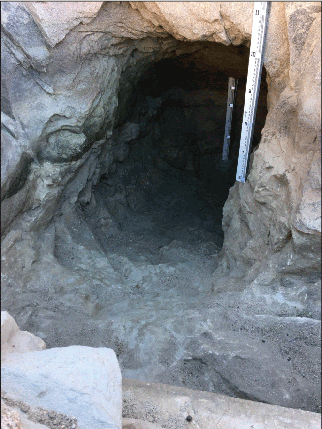
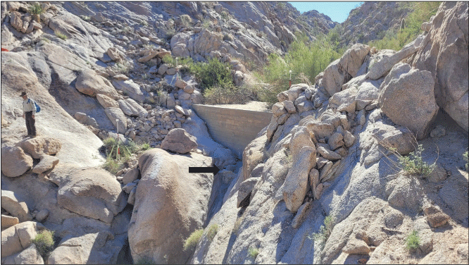
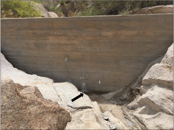
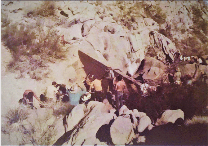
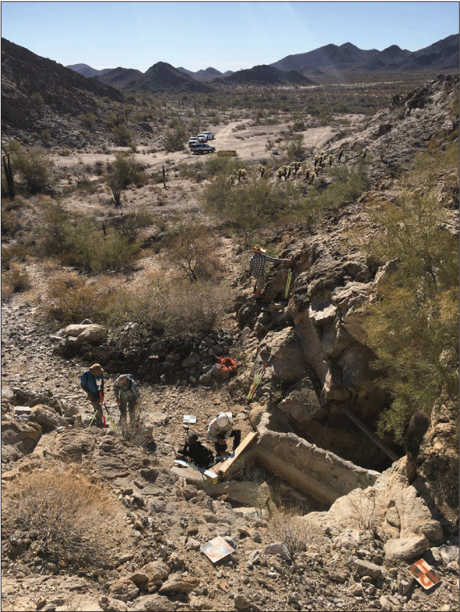
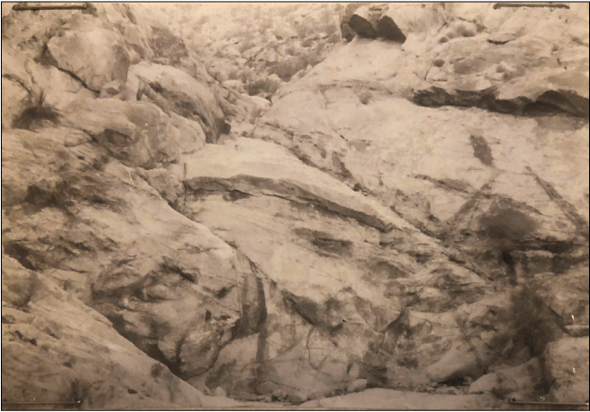
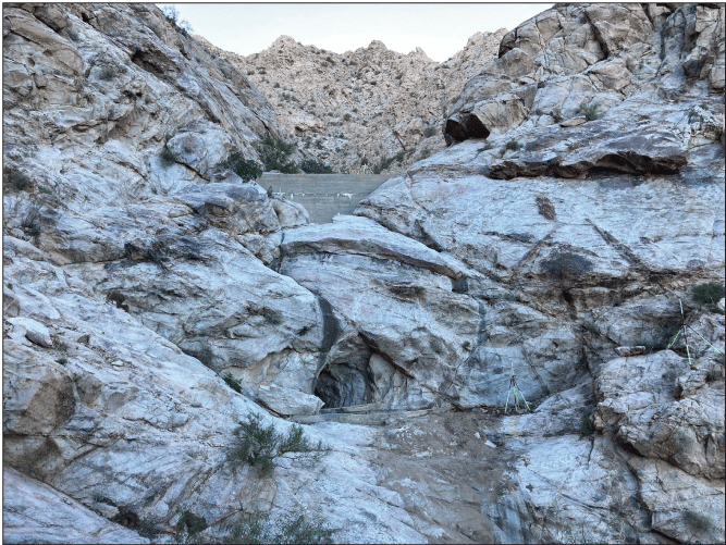
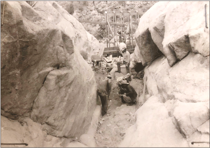
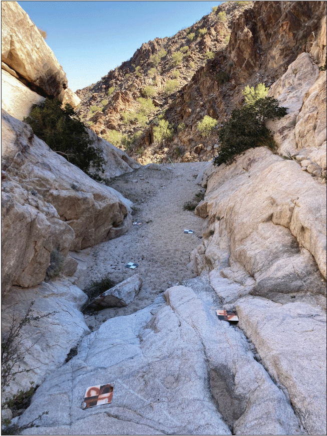
The U.S. Fish and Wildlife Service (USFWS) oversees more than 560 National Wildlife Refuges, many with a Comprehensive Conservation Plan (CCP) outlining goals and objectives to help manage and protect resources such as wildlife and their habitat. One of the resource management objectives of the Cabeza Prieta National Wildlife Refuge (CPNWR) in southern Arizona as stated in the CCP is to sustain a population of 500 to 700 desert bighorn sheep (Ovis canadensis mexicana; USFWS, 2006), which necessitates ensuring free-standing water is available for their consumption. CPNWR is located within the Sonoran Desert where the timing and small amount of annual rainfall limit the availability of natural water supplies for desert bighorn sheep. Water availability is particularly important during the summer months when desert bighorn sheep most commonly visit managed water resources (Harris and others, 2020). To increase water availability for desert bighorn sheep and other wildlife, CPNWR has constructed new, or enhanced existing, bedrock pools that collect rainfall and runoff. The pools are referred to commonly as tanks or tinajas. Modified tanks are naturally occurring water catchments which have been modified by engineering. Constructed tanks are commonly referred to as developed tanks. The water storage basins of developed tanks, created by excavation of rock walls in a runoff catchment, provide water sources in areas that previously lacked these resources (Broyles, 1997). Natural tanks were modified in many ways, generally expanding water storage basins by excavation of adjacent rock walls in natural runoff catchments (Broyles, 1997; fig. 1). The enclosed rock structures of these modified tanks have increased local water storage capacity hundreds to thousands of times beyond their natural capacity, permitting some to become perennial resources (Broyles, 1997).
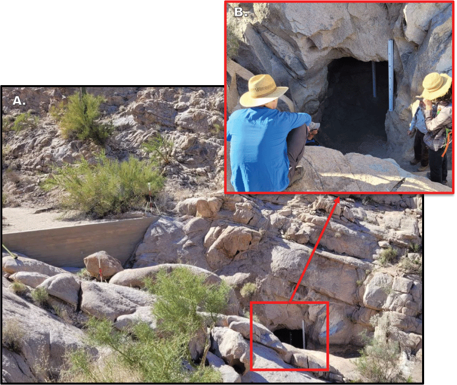
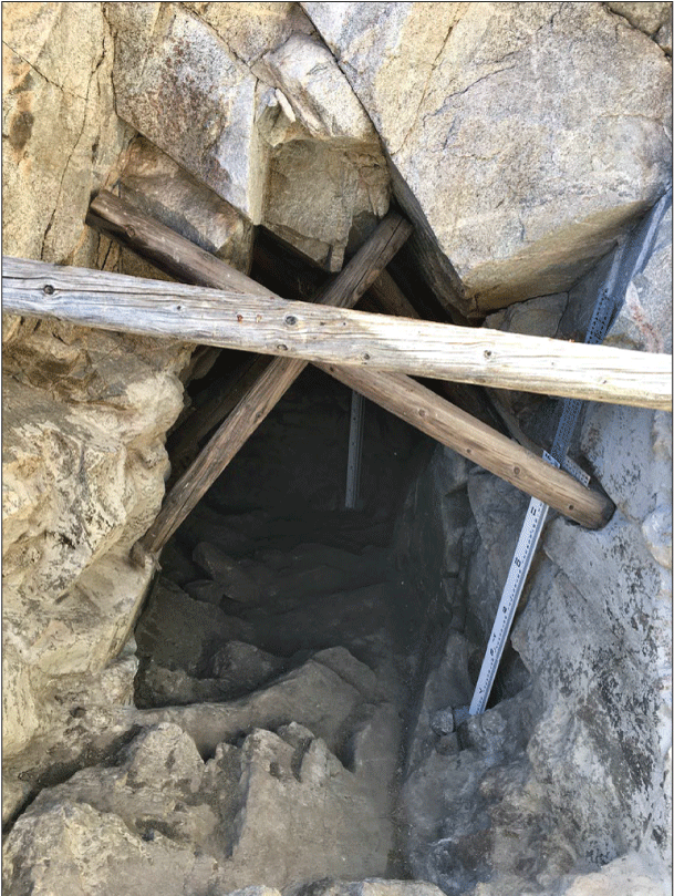
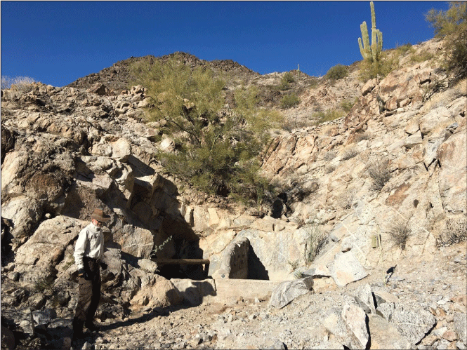
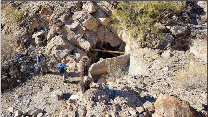
Photographs of Buckhorn Tank, a modified natural tank, in western Cabeza Prieta National Wildlife Refuge, Arizona. Site enhancements include a small sediment retention dam (left side of image A) and a borehole basin into the canyon wall (inset image B). Photographs by J. Caster, U.S. Geological Survey, February 14, 2022.
The relatively low regional precipitation (fig. 2; National Oceanic and Atmospheric Administration [NOAA], 2022) and high evapotranspiration at CPNWR precludes some tanks from filling to their maximum water storage capacity or maintaining a year-round water supply. Therefore, management of tanks as perennial water sources requires some tanks to be mechanically filled by hauling water by truck and trailer. Water hauling operations can be expensive and have effects on wildlife and designated wilderness, such as habitat disruption and increased erosion. In keeping with CPNWR’s goal of wilderness stewardship, also prioritized in the CCP, site visits for resource improvements using motorized vehicles and additional mechanized equipment are to be minimal within wilderness (USFWS, 2006). Management decisions on how often and how much to fill tanks are informed by monitoring estimates of stored water volumes. However, the geometries of the tanks are complex, making estimates of stored water volumes challenging to measure or calculate. Accurate documentation of tank geometry and simplification of calculating volume estimates could better inform management decisions to efficiently meet both wildlife and wilderness stewardship objectives.
The U.S. Geological Survey (USGS) Southwest Biological Science Center, in cooperation with the USFWS during February 2022, employed ground-based light detection and ranging (lidar) to help meet resource management objectives at the CPNWR. Ground-based lidar remote sensing is an efficient and accurate survey tool to measure complex topography and geologic structures like bedrock tanks. Ground-based lidar systems collect millions of spatially explicit topographic measurements in minutes with sub-centimeter (cm) precision. These high-resolution topographic data allow for accurate representations of natural surfaces (Caster and others, 2022) and measurements of confining volumes (Fabbri and others, 2017) without the need to simplify surface geometry into common three-dimensional shapes, such as cylinders. For water catchments, such as tanks, topographic data allow for efficient estimation of how water storage volumes change with water surface elevation (stage height), which is termed a stage-storage model. The lidar-derived data acquired in this study are provided in the associated data release (Caster and others, 2024).
Objectives
In this report we present the results for ground-based lidar survey and analysis of three tanks identified as a priority by CPNWR managers. The purpose of this work was to (1) accurately characterize the complex structure of each tank, and (2) develop a stage-storage model for estimating water storage volumes from simple observations of water surface-stage heights in each tank. Results of this study will permit the refuge to: (1) easily estimate water available for wildlife at any point of time, (2) interpret tank recharge following rainstorms, and (3) make important and potentially expensive management decisions more effective and economical regarding whether and when to transport water via vehicles to mechanically refill the tanks in designated wilderness.
Study Area
CPNWR is in the Sonoran region of the Basin and Range Province of North America, an extensive system of block-fault mountains separated by alluvial valleys. The Sonoran climate is a hot desert, with low temperatures averaging above 0 degrees Celsius (°C) (32 degrees Fahrenheit [°F]) year-round and high temperatures in summer months averaging around 41 °C (107 °F; fig. 2; NOAA, 2022). The distribution of intra-annual precipitation within the region is bimodal, with most of the rainfall occurring from frontal storm systems during the winter months and high intensity convective storms in the summer months that are associated with the North American Monsoon (fig. 2). Although intra-annual rainfall within the region peaks during the summer monsoon season, the high temperature extremes, and hours of sunlight during the summer result in high evapotranspiration potential that limits effective precipitation.
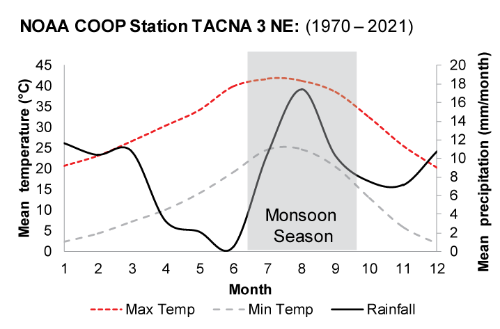
Graph of summaries of mean monthly temperature (Temp) maximums (Max) and minimums (Min) and mean monthly precipitation (rainfall; in millimeters per month [mm/month]), between January 1, 1970, and December 31, 2021, at the Tacna 3 NE National Oceanic and Atmospheric Administration Cooperative Observer Program (NOAA COOP) station USC00028396 located approximately 30 miles north of Buckhorn Tank, in Tacna, Arizona (NOAA, 2022). The window of time during which North American Monsoon activity typically occurs each year from July through September is shown for reference. °C, degree Celsius.
Approximately 93 percent of the refuge (1,255 square miles [mi2]; 3,250 square kilometers [km2]) is designated wilderness containing 24 developed water sources for wildlife. Of these water sources, the refuge identified three tanks as important for desert bighorn sheep for this study: (1) Buckhorn Tank located in the Cabeza Prieta Mountains, (2) Senita Tank in the Drift Hills, and (3) Eagle Tank in the Sierra Pinta (fig. 3). Buckhorn and Eagle Tanks are modified natural tanks whereas Senita Tank is a developed tank (in the sense of Broyles, 1997). However, all three are in natural catchments with man-made shallow bore tunnels (boreholes) into rock walls. All three tanks are also located downstream of a small man-made sediment retention dam constructed during initial modification or development to help reduce sediment infilling and increase water retention in the tank (figs. 1 and 3).
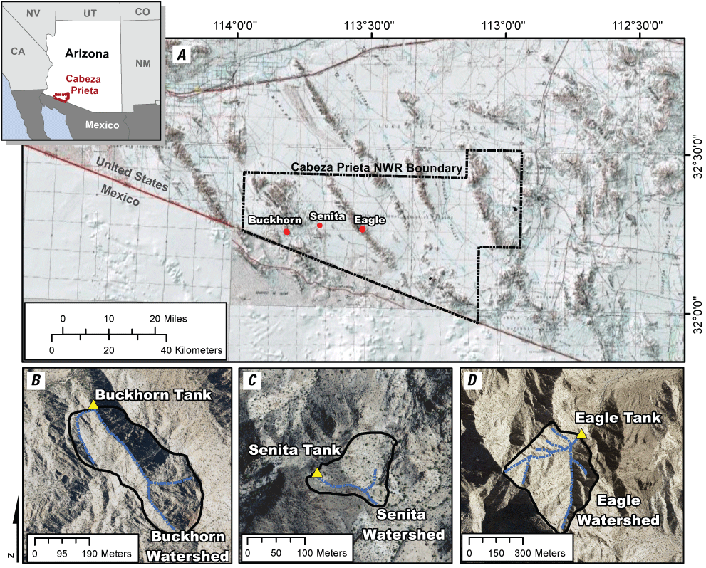
A, Map of the locations (indicated by the red circles) of Buckhorn, Senita, and Eagle Tanks within Cabeza Prieta National Wildlife Refuge (NWR), Arizona. B–D, The tanks (indicated by the yellow triangles) and their respective local contributing watersheds (black outline) with runoff pathways (blue dashed lines). In A, the background topography and imagery is from the U.S. Geological Survey 250,000-scale topographic map series, and in B–D, the 2019 aerial imagery is from the U.S. Department of Agriculture for the National Agricultural Imagery Program courtesy of the U.S. Geological Survey (https://earthexplorer.usgs.gov; Earth Resources Observation and Science [EROS] Center, 2018).
Buckhorn Tank is a modified natural tank located within the National Hydrography Dataset (NHD; Seaber and others, 1987) sub-watershed (HUC-12) of Tule Well, which drains local precipitation southwest into Mexico. The upstream contributing area for Buckhorn Tank is approximately 0.12 km2 (30 acres) of rocky, mountainous terrain with an average slope of 27 degrees and runoff channels up to half a kilometer in length (about 0.3-mile long, fig. 3). The tank was initially modified in 1949, which included construction of a concrete liner wall to seal off a rock fault and elevate the pour point by 2 feet (ft) (USFWS, 1950). In 1976, the tank was completely cleaned out, the sediment trap was partially cleaned out, and additional improvements were made. Improvements included sealing the tank with a Thoroseal and Acryl 60 plaster mix and construction of a small masonry dam at the outside edge of the concrete liner wall to prevent sediment from backflowing into the tank (Dodson, 1976a; USFWS, 1977); this higher pour point also increased the tank’s capacity. The tank was completely cleaned out and the sediment trap was partially cleaned out again in 2003 (Tracey Martin, Arizona Desert Bighorn Sheep Society, personal commun., September 9, 2022). Buckhorn tank has the largest capacity of the three tanks included in this study, which was originally reported as 30,250 liters (L) (7,991.2 gallons [gal]) (USFWS, 1950) and after addition of the masonry rock dam estimated to be 37,850 L (9,998.9 gal) by Broyles (1997).
Senita Tank is a developed tank in the Mohawk wash NHD HUC-12 sub-watershed, which drains northeast. Relative to the other tanks studied, Senita Tank has the smallest upstream contributing area of approximately 0.12 km2 (3.8 acres). This upstream contributing area also has the shallowest average slope of 21.6 degrees and shortest runoff channels (0.15 kilometers [km], [492 ft]; fig. 3). Senita Tank was constructed in 1958 (USFWS, 1958b) and improved in 1974 (USFWS, 1975) to have a capacity of 26,495 L (6,999.2 gal) as reported by Broyles (1997). Improvements included removal of debris and application of a Thoroseal and Acryl 60 plaster mix to seal the tank (Dodson, 1976b). In 1976, the upper runoff catchment and small masonry dam at the entrance were sealed with the plaster mix (Dodson, 1976b).
Eagle Tank is a modified natural tank in the Hummingbird Canyon NHD HUC-12 sub-watershed, which drains east into the Mohawk Valley. Eagle Tank has an upstream contributing area of approximately 0.18 km2 (45 acres) with an average slope of 35 degrees and runoff channels over half a kilometer in length (fig. 3). The tank was modified in 1957 to a capacity originally reported as 24,605 liters (6,500.0 gal) (USFWS, 1958a) and later estimated as 24,602 liters (6,499.2 gal) by Broyles (1997). No evidence has been found on site or in the CPNWR’s annual narratives indicating the tank and upstream sediment retention dam have been improved or cleaned out since construction.
Materials and Methods
Field Surveys
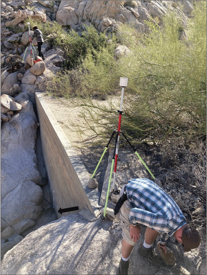
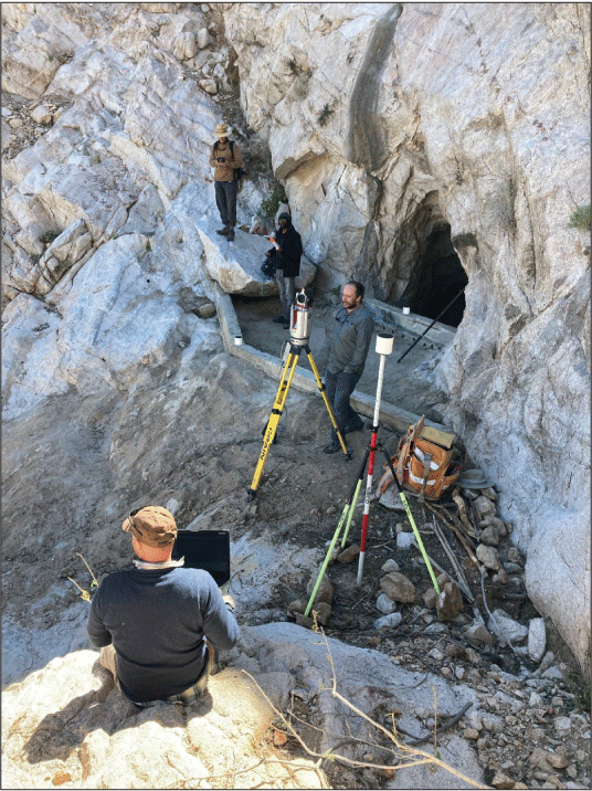
We surveyed each tank, and the adjacent area upstream and downstream, using ground-based lidar and real-time kinematic global positioning system and global navigation satellite systems (RTK-GPS/GNSS) (fig. 4). The lidar surveys used a Riegl VZ1000 laser scanner with a mounted Nikon D810 digital camera (fig. 4) to acquire photo-colorized topographic measurements with a median density greater than (>) 500 points-per-square meter. We conducted lidar scans from multiple stationary positions to better capture the complexity of the terrain, registering each scan position with four to eight stationary reflective ground control targets. The positions of the ground control targets were surveyed with a Trimble R8 RTK-GPS/GNSS rover and base station receiver pair and were used to georeference the lidar topographic data. National Geodetic Survey (NGS; https://geodesy.noaa.gov/index.shtml) published survey control benchmarks were not available within the vicinity of the sites. A location was selected at each site to deploy the base station receiver and the spatial data were referenced to the National Spatial Reference System (NSRS) by post-processing of at least 3 hours of static GNSS observables through the NGS’s Online Positioning User Service (OPUS, https://www.ngs.noaa.gov/OPUS/). The results classify the data as USGS Level III GNSS positioning (Rydlund and Densmore, 2012). Vertical coordinate information of the RTK-GPS/GNSS survey and georeferenced lidar data is referenced to the North American Vertical Datum of 1988 (NAVD 88) and used the geoid model Geoid18. Horizontal coordinate information is referenced to the 2011 adjustment of the North American Datum of 1983 (NAD 83 [2011]) and used the cartesian coordinate system NAD 83 (2011), Universal Transverse Mercator (UTM) zone 12N (Rydlund and Densmore, 2012).
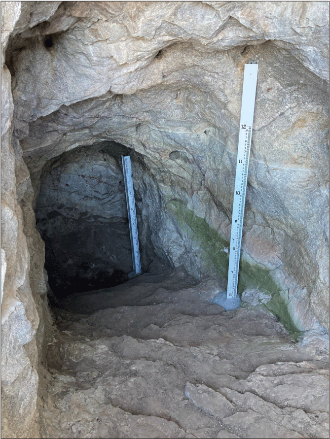
Prior to each survey, CPNWR staff pumped out and temporarily stored water from each tank and then removed sediment that had infilled since modification, development, or subsequent improvement. Next, to measure stage height, CPNWR staff installed fixed rods marked from 0 ft to 12 ft (Buckhorn and Eagle Tanks) or 14 ft (Senita Tank) at 1/10-ft intervals from the bottom of each tank (fig. 4A). These preparations allowed the survey to characterize the full capacity of each tank with lidar and provided a height reference for estimating stage-storage capacity relationships.
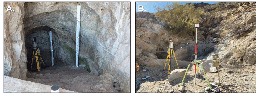
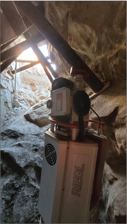
Images of Eagle and Senita Tanks, Cabeza Prieta National Wildlife Refuge (CPNWR), Arizona. Prior to each survey, CPNWR staff pumped out and temporarily stored water from each tank and then removed sediment that had infilled since modification, development, or subsequent improvement. Next, to measure stage height, CPNWR staff installed fixed rods marked from 0 feet (ft) to 12 ft (Buckhorn and Eagle Tanks) or 14 ft (Senita Tank) at 1/10-ft intervals from the bottom of each tank. A, Lidar instrument (Riegl VZ1000) in Eagle Tank next to fixed rods for measuring stage height. B, Lidar instrument and 4-inch (10-centimeter) diameter cylindrical reflective control target mounted on tripod outside of Senita Tank. Photographs by J. Caster, U.S. Geological Survey, February 15, 2022.
Data Analysis
The lidar echo return measurements, termed a point cloud, were prepared for analysis by first colorizing and georeferencing the data in RiSCAN PRO software (http://www.riegl.com/products/software-packages/riscan-pro/; accessed August 1, 2024). Average scan-to-scan registration error between targets was 0.5 cm. Lidar-to-GPS registration errors averaged 0.7 cm. The average GPS solution error was 1.4 cm, and the average horizontal and vertical GPS position error is 0.6 cm and 1.2 cm, respectively. We thus estimate the total positional uncertainty as 2.1 cm based on analysis of the sum of squared errors in quadrature, that is:
We segmented the georeferenced point cloud data to classify data points as either bare earth, vegetation, or our survey equipment, including the tank stage height rods, using an iterative height filter and manual selection. We then used the bare-earth dataset (which included the rock surfaces inside the tank) to analyze the geometric dimensions and storage capacity of each dry tank as well as the associated sediment retention dam directly upstream.
Tank Stage-Storage Capacity
Using the bare-earth point cloud of each tank, we evaluated the maximum storage capacity as well as stage-storage capacity for 1 ft, 2 ft, 4 ft, 6 ft, 8 ft, and 10 ft stage heights (fig. 5B). The maximum tank storage capacity was defined by the area below the pour point elevation at the downstream side of the tank basin. The pour point, or the outlet for water draining out of the tank, was defined by a concrete wall surrounding the main basins for both Senita and Eagle Tanks. The Buckhorn Tank maximum storage capacity included the area above the concrete liner enclosed by the small masonry dam added in 1976. Stage-storage capacity was defined by the elevations of the six stage heights (that is 1, 2, 4, 6, 8, and 10 ft) from the installed stage height rods within the tanks.
Stage-storage capacity can be calculated directly from the bare-earth classified points or from derived GIS products, such as an interpolated surface raster (grid cells) and triangulated-irregular networks (TINs). Each method has the potential to introduce interpolation errors. To account for this, we carried out point-based, raster-based, and TIN-based volume calculations for each stage height and report the mean and 95 percent confidence interval of the mean of the three methods for each tank.
The point and raster-based methods are the most common approaches to estimate reservoir volume, in which basin elevations are subtracted from water fill elevations at each measurement point and the differences are summed to estimate a volume for the entire reservoir. These methods have the benefit of providing a spatially explicit representation of stage heights that allow for validation and visualization. We carried out the point-based storage capacity estimate in CloudCompare (version 2.10.2; CloudCompare, 2019) by first separating the tank point cloud below the maximum fill elevation into two datasets, one representing the highest elevation, hereafter the ceiling, and one representing the lowest elevation submerged by water, hereafter the ground (fig. 5D). At higher stage heights, a portion of the tank’s overlying rock was lower than the stage elevation. In these cases, we used the maximum elevation of the rock within a 5-cm moving window as the ceiling. In other cases, the ceiling was defined by the maximum or stage height elevation. The ground dataset was defined by the minimum elevation within a 5-cm moving window. The ground was subtracted from the ceiling to get a positive volume reported in cubic meters (m3).
We used the ceiling and ground point-cloud datasets to create 5-cm resolution digital elevation models (DEMs) that were used in the raster-based stage-storage capacity estimate. A 5-cm resolution was selected for DEM analysis as it provided sufficient detail to capture surface complexity while reducing noise introduced by differences within the horizontal footprint of the ceiling and ground. The DEMs were imported to Esri ArcGIS version 10.7 and differenced as they were with the point cloud datasets (Caster and others, 2022). The resulting raster was summarized using zonal statistics within the two-dimensional planar footprint of the tank’s ground DEM to estimate storage capacity.
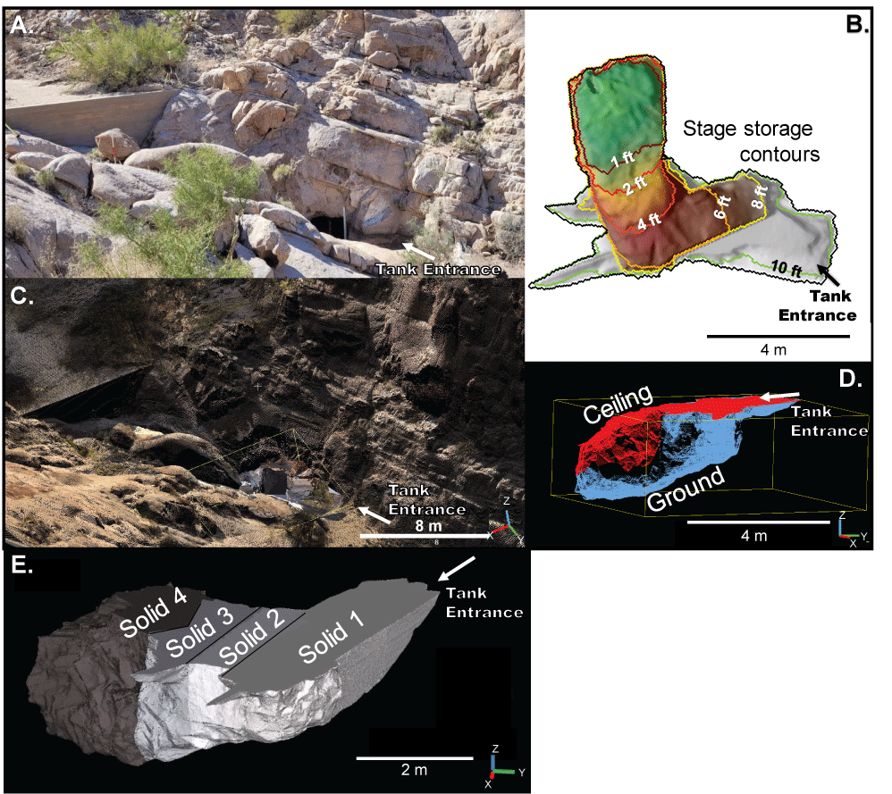
Photographs and diagrams of tank stage-storage capacity survey and analysis products at Buckhorn Tank, a modified natural tank in Cabeza Prieta National Wildlife Refuge, Arizona. A, Field photograph of Buckhorn Tank and upstream sediment retention dam. B, Diagram of interpreted stage-height contours within the spatial extent of storage capacity. The entrance into the developed portion of the tank is identified for reference. C, Lidar point-cloud with natural colorization applied from photographs covering the full extent of the surfaces within part A. A wire frame box marks the source of data used in parts D and E. D, Diagram of the maximum storage capacity point cloud for Buckhorn Tank split into an upper (red) and lower (blue) dataset for measuring capacity through surface differencing. E, Four mesh objects used to calculate a solid volume for the developed portion of Buckhorn Tank. Photographs by J. Caster, U.S. Geological Survey, February 14, 2022. ft, foot; m, meter.
We calculated the TIN-based volume estimate in Maptek PointStudio (Maptek PointStudio version 8.1; https://www.maptek.com/; accessed August 1, 2024) as a solid model of a reservoir. A solid model is created by defining a central location within the void space of the point cloud, which is used as a node to build facets at the distal extents of the point cloud. Solid model construction requires non-overlapping features from the perspective of the central node to accurately define radial distance relationships that are used for volume estimates. We subset the point cloud by stage height to eliminate overlapping areas and then combined the products to ensure the most accurate capacity estimates (see for example, fig. 5E).
We developed a stage-storage model for each tank as a best fit relationship between the mean of the volume estimates from the three methods and the stage heights. In addition to linear regression models, we evaluated power, exponent, log, and second-order polynomial model fitting functions. For models with an R-square value >0.9, we selected the best model as the most parsimonious equation with the lowest root mean square error (RMSE). We additionally developed a stage and water storage surface area model for each tank and those are presented in appendix 1.
Sediment Retention Dam Storage
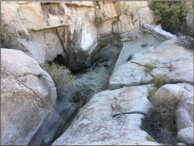
In addition to the tank fill volumes, we investigated potential sediment trapped behind the upstream dam and calculated the remaining storage capacity of the impounded reservoir. During field surveys, we did not conduct subsurface testing to estimate sediment depths or porosities behind the sediment retention dams. To approximate sediment volume, we interpolated a channel bed using the slope and geometry of the surrounding banks and channel above and below the dam to estimate a hypothetical base elevation. Using the point-based method (described in subsection “Tank Stage-Storage Capacity”), we then subtracted the interpolated base from the point cloud measurements at the channel surface for the area we identified as unconsolidated sediment (fig. 6). This estimate of sediment volume approximates the combined volume of space filled by sediment and by pores (voids) in the sediment deposit that can be potentially filled with air or water.
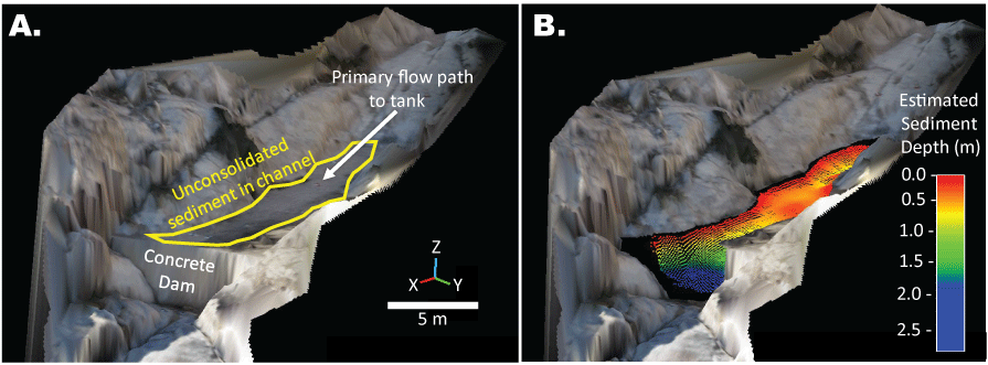
Diagram of the method for estimating sediment retention behind the upstream dam at Eagle Tank, a modified natural tank, Cabeza Prieta National Wildlife Refuge, Arizona. A, A Triangulated Irregular Network (TIN) mesh colored from natural-colored photographs for the sediment retention dam and upstream channel above the tank. The extent of the concrete dam and unconsolidated sediment were determined by photographic interpretation. B, TIN mesh with an interpolated channel base elevation. Estimated sediment depth in meters (m) was determined from the elevation difference between the unconsolidated sediment surface and the interpolated channel base.
Next, we used the elevation at the top of the dam to estimate the remaining void space above the current sediment surface but below the dam that could, for example, be filled in the future by sediment or water. To do this, we first subtracted the surface elevations for the area upstream of the dam from the elevation at the top of the dam. We next summarized the positive values within the channel bed to estimate the remaining storage capacity of the sediment retention dams upstream of each of the tanks.
Results
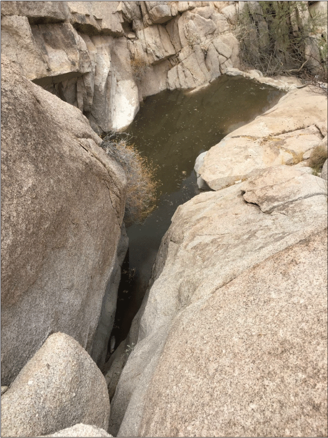
The lidar point cloud for each survey site covered the tank and a portion of the up and downstream area leading to and from the tanks (for example, fig. 7) that are provided in a separate data release (Caster and others, 2024). This included about 38 percent of the upstream contributing watershed area for Buckhorn Tank, around 90 percent of Senita Tank’s contributing watershed, and less than 5 percent of Eagle Tank’s contributing watershed. At all three sites, the lidar survey captured almost all the channel draining from the tank to an arroyo in the downstream valley, as well as the staging area for water trucks and the temporary water storage tanks. Visual comparisons of this survey data with the most recent aerial photographs acquired in 2019 for the U.S. Department of Agriculture (USDA) National Agricultural Imagery Program (NAIP) (Earth Resources Observation and Science [EROS] Center, 2018; https://earthexplorer.usgs.gov) demonstrated that each survey aligns well with other national datasets and could be useful for further watershed analysis.
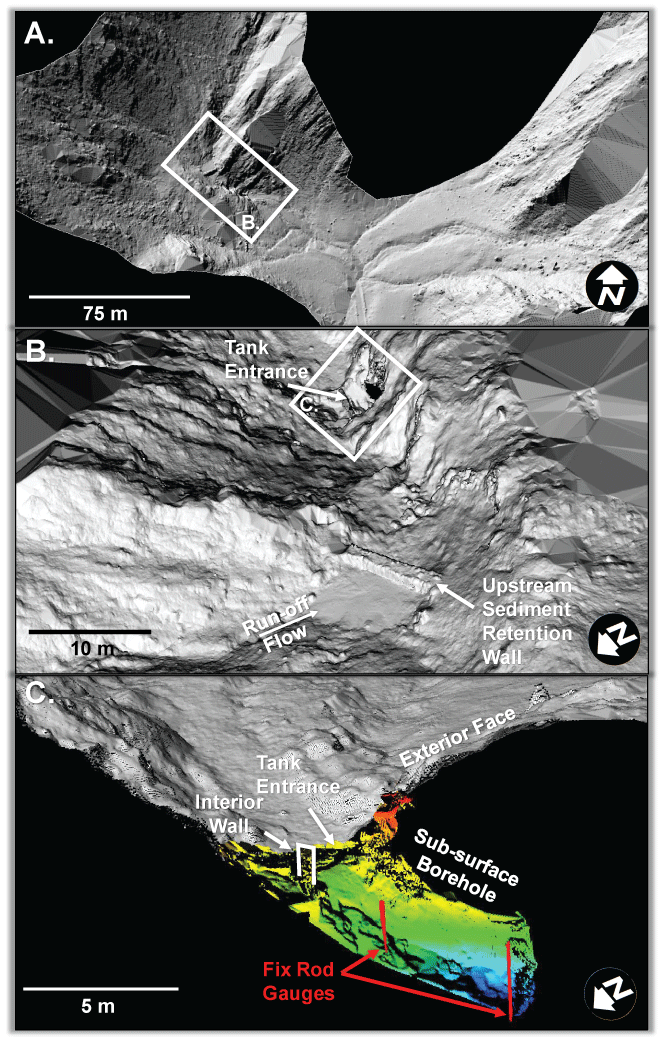
Topographic relief model for Senita Tank, a developed tank, including a portion of the upstream and downstream areas leading to and from the tank, Cabeza Prieta National Wildlife Refuge, Arizona. A, Hillshade relief of the Senita Tank 20-centimeter-per-pixel resolution lidar triangulated irregular network (TIN). B, Zoomed in, oblique view of the 5-centimeter-per-pixel resolution lidar TIN. C, Profile view of the Senita Tank point cloud within the 5-centimeter-per-pixel resolution TIN relief. In panel C, the tank borehole below ground is colored by relative height, with cool colors (blue and green) representing lower elevations and warm colors (yellow and red) higher elevations. m, meter.
Tank Capacity
The mean-stage storage capacities for each tank are provided as tabular data in the following subsections “Buckhorn Tank,” “Senita Tank,” and “Eagle Tank” (tables 1–3). In the tables, we present the mean capacities calculated from the point, raster, and TIN-based measurement methods in m3, liters (L), and gallons (gal; tables 1–3). Error estimates in the tables are unitless, provided as percentages of the mean stage-storage capacities, so that they can be more easily applied to any given unit of capacity. For ease of application in the field by the refuge managers, we present the results of the stage-storage capacity, the upper and lower bounds of the 95 percent confidence intervals, and the stage-storage model equations in gallons.
For all three tanks, the TIN-based solid volume method was consistently the smallest estimate of storage capacity (tables 1–3). The point and raster-based surface differencing methods produced more similar capacity estimates, though the point-based method estimates tended to be larger (tables 1–3). These differences were relatively small and resulted in an average standard error (SE) of measurements for Buckhorn, Senita, and Eagle Tanks of 1.8 percent, 2.3 percent, and 1.7 percent, respectively. The upper and lower bounds of estimated capacity as represented by the 95 percent confidence intervals for Buckhorn, Senita, and Eagle averaged plus or minus (±) 3.6 percent, 4.5 percent, and 3.4 percent of stage-storage capacity, respectively.
Buckhorn Tank
Buckhorn Tank, a modified natural tank, had the largest capacity of the three tanks included in this report, with a maximum storage capacity of 9,108.730±252.312 gal (table 1, fig. 8). The original portion of the tank, the volume of the rock borehole below the top of the concrete liner, represented a stage height of approximately 9 ft with a storage capacity of 7,192.540±201.391 gal (table 1, fig. 8). Using these measurements and the additional stage capacities in table 1, stage storage was best modeled using either a power or polynomial equation, both of which had coefficient of determination (R2) values >0.99. However, the second-order polynomial equation, BHSgal (Buckhorn Tank Stage-Storage Model in water-storage units of gallons; fig. 8), had the lowest RMSE at 59.9 gal with an average residual <1 percent of measured capacity. Applying the BHSgal stage-storage model, we approximate the stage heights at which Buckhorn Tank is at half and one-quarter capacity (that is, 50 percent and 25 percent full, respectively) are 6.4 ft and 3.8 ft, respectively. The model predicts that stage-storage drops below 100 gal at a stage height of 0.5 ft.
Table 1.
Results of stage-storage volume estimation for Buckhorn Tank, a modified natural tank in Cabeza Prieta National Wildlife Refuge, Arizona.[Mean stage-storage capacity represents the average storage capacity of the point, raster, and triangulated irregular network (TIN)-based measurement methods (described in “Tank Stage-Storage Capacity” section) at each stage height determined by a fixed rod within the tank. Note that the 9.0-foot (ft) stage height corresponds with the original capacity of the tank when filled to the top of the concrete liner, and the maximum capacity includes the shallow entrance into the tank, enclosed by a small masonry dam, above the liner. To facilitate use of each metric, the standard error (SE) and 95 percent (%) confidence interval (CI) are provided as a percentage of the mean stage-storage capacity. For ease of reference, mean stage-storage capacity is provided in the original measurement units: ft, foot; m3, cubic meter; L, liter; gal, U.S. gallon. For the graph of the stage-storage model see figure 8.]
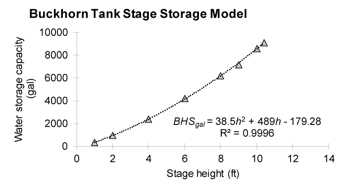
Graph of stage-storage model for Buckhorn Tank, a modified natural tank in Cabeza Prieta National Wildlife Refuge, Arizona. The polynomial equation, BHSgal, estimates stage storage in U.S. gallons (gal) from the fixed rod stage height (h) within Buckhorn Tank. Note that the 9.0-foot (ft) stage height corresponds with the original capacity of the tank when filled to the top of the concrete liner wall, and the maximum capacity (table 1) includes the shallow entrance into the tank, enclosed by a small masonry dam that extends above the wall. We approximate the stage heights at which Buckhorn Tank is at half and one-quarter capacity as 6.4 ft and 3.8 ft, respectively. For the results of stage-storage volume estimations see table 1. R2, coefficient of determination.
Senita Tank
Senita Tank is a developed tank that is 485 gal smaller than Buckhorn Tank, with a maximum storage capacity of 8,623.308±226.793 gal (table 2, fig. 9) at an estimated stage height of 13 ft. Using the stage capacities in table 2, we modeled stage storage using a second-order polynomial equation, SNSgal (Senita Tank Stage-Storage Model in water storage units of gallons; fig. 9), that had an R2 value of 0.9991. SNSgal had an RMSE of 84.4 gal with an average residual of 12.8 percent of measured capacity (fig. 9). Residual errors for SNSgal were greatest at 1 ft, where the model underpredicts storage capacity by 61 percent (30.9 gal). At 2 ft stage heights and higher, the model better predicts stage storage with an average residual of 4.7 percent. Applying the SNSgal stage-storage model, we approximate the stage heights at which Senita Tank is at half and one-quarter capacity are 8.8 ft and 5.9 ft, respectively. The model predicts that stage-storage drops below 100 gal at a stage height of 1.2 ft.
Table 2.
Results of stage-storage volume estimation for Senita Tank, a developed tank in Cabeza Prieta National Wildlife Refuge, Arizona.[Mean stage-storage capacity represents the average storage capacity of the point, raster, and triangulated irregular network (TIN)-based measurement methods (described in section “Tank Stage-Storage Capacity”) at each stage height determined by a fixed rod within the tank. To facilitate use of each metric, the standard error (SE) and 95 percent (%) confidence interval (CI) are provided as a percentage of the mean stage-storage capacity. For ease of reference, mean storage capacity is provided in the original measurement units: ft, foot; m3, cubic meter; L, liter; gal, U.S. gallon. For the graph of the stage-storage model see figure 9.]
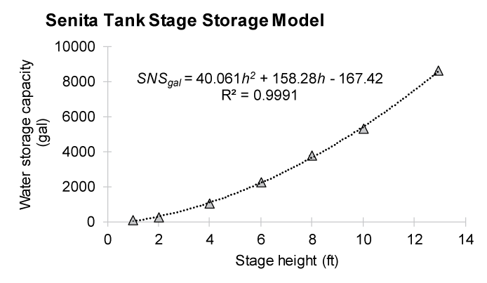
Graph of the stage-storage model for Senita Tank, a developed tank in Cabeza Prieta National Wildlife Refuge, Arizona. The polynomial equation, SNSgal, estimates stage storage in U.S. gallons (gal) from the fixed rod stage height (h) within Senita Tank. This tank has a maximum storage capacity of 8,623.308±226.793 gal at an estimated stage height of 13 feet (ft). We approximate the stage heights at which Senita Tank is at half and one-quarter capacity as 8.8 ft and 5.9 ft, respectively. The model predicts that stage-storage drops below 100 gal at a stage height of 1.2 ft. For the results of stage-storage volume estimations see table 2. R2, coefficient of determination.
Eagle Tank
Eagle Tank is a modified natural tank and the smallest tank examined in this report, with a maximum storage capacity of 6,039.603±120.188 gal (table 3, fig. 10) at an estimated stage height of 10.6 ft. Using the stage capacities in table 3, we modeled stage-storage using a 2nd order polynomial equation, EGSgal (Eagle Tank Stage Storage-Model in water storage units of gallons; fig. 10), that had an R2 value of 0.9987. EGSgal had an RMSE of 79.7 gal with an average residual of 3.1 percent of measured capacity (fig. 10). Applying the EGSgal stage storage-model, we approximate the stage heights at which Eagle Tank is at half and one-quarter capacity are 7.6 ft and 5.3 ft, respectively. The model predicts that stage storage drops below 100 gal at a stage height of 1.3 ft.
Table 3.
Results of stage-storage volume estimation for Eagle Tank, a modified natural tank in Cabeza Prieta National Wildlife Refuge, Arizona.[Mean stage-storage capacity represents the average storage capacity of the point, raster, and triangulated irregular network (TIN)-based measurement methods (described in section “Tank Stage-Storage Capacity”) at each stage height determined by a fixed rod within the tank. To facilitate use of each metric, the standard error (SE) and 95 percent (%) confidence interval (CI) are provided as a percentage of the mean stage-storage capacity. For ease of reference, mean storage capacity is provided in the original measurement units: ft, foot; m3, cubic meter, L, liter; gal; U.S. gallon. For the graph of the stage-storage model see figure 10.]
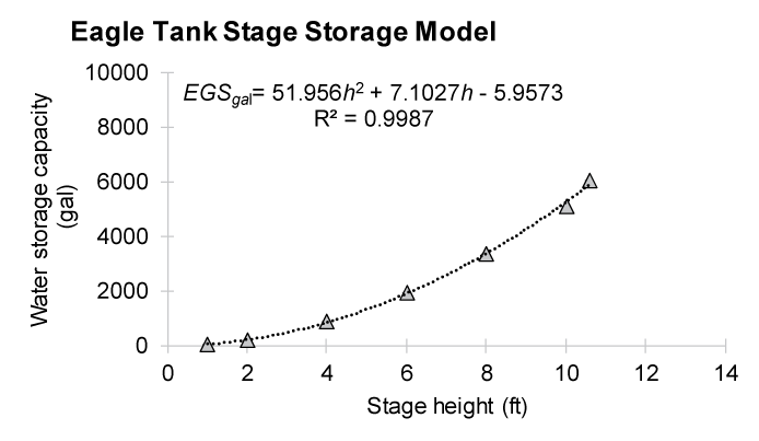
Graph of stage-storage model for Eagle Tank, a modified natural tank in Cabeza Prieta National Wildlife Refuge, Arizona. The polynomial equation, EGSgal, estimates stage storage in U.S. gallons (gal) from the fixed rod stage height (h) within Eagle Tank. We approximate the stage heights at which Eagle Tank is at half and one-quarter capacity are 7.6 feet (ft) and 5.3 ft, respectively. The model predicts that stage-storage drops below 100 gal at a stage height of 1.3 ft. For the results of stage-storage volume estimations see table 3. R2, coefficient of determination.
Sediment Storage
Each of the sediment retention dams for the tanks was built at a head cut within a tributary channel. At all three tanks, the upstream and downstream portions of the channel beds are bedrock, except for the areas directly upstream of the dams that have alluvial unconsolidated sediment. Although we do not have documentation of the channel bed before dam construction at Buckhorn Tank, it is probable that much of the alluvial sediment was deposited on bedrock after dam construction. Photographic documentation at Senita Tank suggests about half of the pre-dam channel was bedrock and half alluvial unconsolidated sediment (USFWS, 1958b; appendix 2, fig. 2.21). Photographic documentation at Eagle Tank suggests that much of the pre-dam channel bed was bedrock, although sand immediately upstream of the concrete dam was used to make the concrete (USFWS, 1958a; appendix 2, figs. 2.27–29). Based on these assumptions, observations, and our interpolated bedrock channel bases, we estimate the volumes of the sediment deposits (combined volume of sediment and pore spaces) currently retained by the dams above Buckhorn, Senita, and Eagle Tanks are approximately 37.79 m3 (49.43 cubic yards [yd3]), 5.80 m3 (7.59 yd3), and 31.99 m3 (41.84 yd3), respectively (table 4).
We can also speculate about sedimentation rates behind each dam with the following assumptions: (1) sediment behind each dam had not been removed since construction at Senita and Eagle Tanks or since the last recorded improvement at Buckhorn Tank; and (2) new sediment is still being retained by the dams. An important caveat associated with the second assumption is that because sediment retention by the dams at both Buckhorn and Eagle Tanks are currently at or very close to capacity, estimated rates of sedimentation are probably underpredicted for both sites.
Buckhorn has the highest estimated average sedimentation rate at 2.1 m3/year (2.75 yd3/year), followed by Eagle Tank at 0.49 m3/year (0.64 yd3/year) (table 4). Senita Tank has the lowest estimated average sedimentation rate at 0.09 m3/year (0.12 yd3/year) (table 4), possibly resulting from a smaller upstream contributing area in comparison to the other tanks. For Buckhorn, the estimated average annual sedimentation rate exceeds the measured remaining surface storage capacity of 0.32 m3 (0.42 yd3/year) by several orders of magnitude, indicating that new sediment inputs are probably not trapped behind the retaining wall and are instead transported over the wall of the dam and deposited in the tank below; this also appears to be corroborated by the sediment that CPNWR had to remove from the tank prior to conducting the lidar surveys for this report. The remaining surface-storage capacity above Eagle Tank’s sediment retention dam is less than two times larger than the estimated average annual sedimentation rate and channel flow depths of 5 cm (approximately 2 inches) or greater could potentially overtop it. The dam at Eagle Tank is located upstream of an overhang above the tank. Because of the position of the tank relative to the dam, much of the sediment transported over the dam is probably not deposited in the tank but instead accumulates in an external modified basin separated from the excavated borehole by a short concrete wall with numerous drainpipes. In contrast, the remaining surface capacity for the sediment retention dam above Senita Tank is several orders of magnitude greater than the estimated sediment volume, likely indicating that upstream flood sediment is trapped behind the sediment retention dam and not deposited in the developed tank.
Table 4.
Estimates of sediment retention and remaining capacity above the sediment retention dam upstream of selected tanks, Cabeza Prieta National Wildlife Refuge, Arizona.[Interpolated sediment volume represents the difference between the unconsolidated sediment surface in the channel bed and the interpolated bedrock below. Remaining capacity represents the difference in volume between the elevation at the top of the dam and the channel bed. For Senita and Eagle Tanks, the tank development year from Broyles (1997) is assumed as the date of dam construction and initiation of channel infilling. m3, cubic meter; yd3, cubic yard; yr, year]
Discussion
The U.S. Fish and Wildlife Service estimated the maximum water storage capacity of Buckhorn and Eagle Tanks after they were modified in 1949 and 1957, respectively, but there is not a similar record that we are aware of for Senita Tank after it was developed in 1958 (table 5). Maximum water storage capacity was later estimated for all three tanks by Broyles (1997) using a common geometric simplification termed conical volume. Broyles’ (1997) estimate of maximum water storage capacity for Eagle Tank only differed by 0.8 gal from the estimate by USFWS (1958a; table 5). However, Broyles’ (1997) estimate for maximum water storage capacity of Buckhorn Tank differed by 2,007.7 gal from the estimate by USFWS (1950; table 5). This discrepancy is likely due to the initial project lacking the small masonry dam at the edge of the concrete liner, which increased the capacity of the tank. Our estimate of capacity at 9 ft, likely the original maximum storage capacity of the tank, is 10 percent lower than the 1950 estimate.
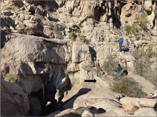
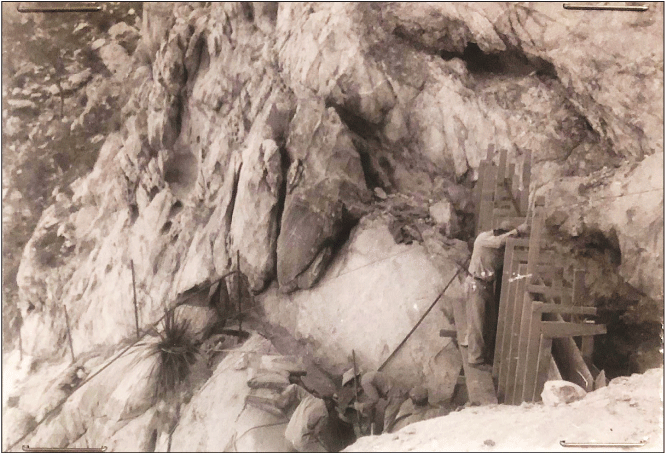
We achieved Objective 1 by using ground-based lidar to refine these estimates of water storage capacities. We measured Buckhorn and Eagle Tanks to have a 9 percent and 7 percent smaller capacity, respectively, and Senita Tank to have a 23 percent greater capacity than previously reported by Broyles (1997; table 5). The percent differences in capacity estimates for Buckhorn and Eagle compared to Broyles (1997) meets our expectations for comparing volume calculation methods that incorporate different levels of geometric complexity, as indicated by percent standard error and 95-percent confidence interval among three different measurement methods used in this study. However, the 23 percent difference between the ground-based lidar volume estimate and the conical volume for Senita Tank previously reported by Broyles (1997) is greater than our expectation for methodological differences. We think that the difference is because a small-walled catchment that was used to convey runoff was included in our ground-based lidar calculations but may not have been considered by Broyles (1997; fig. 11). Using a stage height of 11 ft, which mostly excludes the walled catchment in the lidar data, models a stage-storage capacity of 6,421.041 gal (24,306.28 L), which is 8 percent different from conical volume estimates (fig. 11). It is also possible that a portion of the catchment was filled with sediment during the survey by Broyles (1997). These results show that the accuracy of the previous estimates of the maximum storage capacity for 49 perennial water sources by Broyles (1997) needs to be considered carefully prior to contemporary use. Factors such as tank geometric complexity may produce significant differences between lidar-based and conical volume estimation methodologies and documented or undocumented changes to tank capacity caused by sedimentation or management modifications may further increase these discrepancies.
Table 5.
Comparison of maximum storage capacity of Buckhorn, Senita, and Eagle Tanks across studies, Cabeza Prieta National Wildlife Refuge, Arizona.[Maximum (max) storage capacity refers to the volume enclosed below the pour point at the downstream end of the tank. USFWS, U.S. Fish and Wildlife Service; USGS, U.S. Geological Survey; m3, cubic meter; L, liter; gal, gallon; —, unevaluated. USGS max capacity calculated for 2022 in this study]
| Tank | USFWS (1950; 1958a, b) max capacity | Broyles (1997) max capacity | USGS max capacity | ||||||
|---|---|---|---|---|---|---|---|---|---|
| m3 | L | gal | m3 | L | gal | m3 | L | gal | |
| Buckhorn | 30.250 | 30,250 | 7991.2 | 37.850 | 37,850 | 9998.9 | 34.48030 | 34,480.30 | 9108.730 |
| Senita | — | — | — | 26.495 | 26,495 | 6999.2 | 32.64278 | 32,642.78 | 8623.308 |
| Eagle | 24.605 | 24,605 | 6500.0 | 24.602 | 24,602 | 6499.2 | 22.86239 | 22,862.39 | 6039.603 |
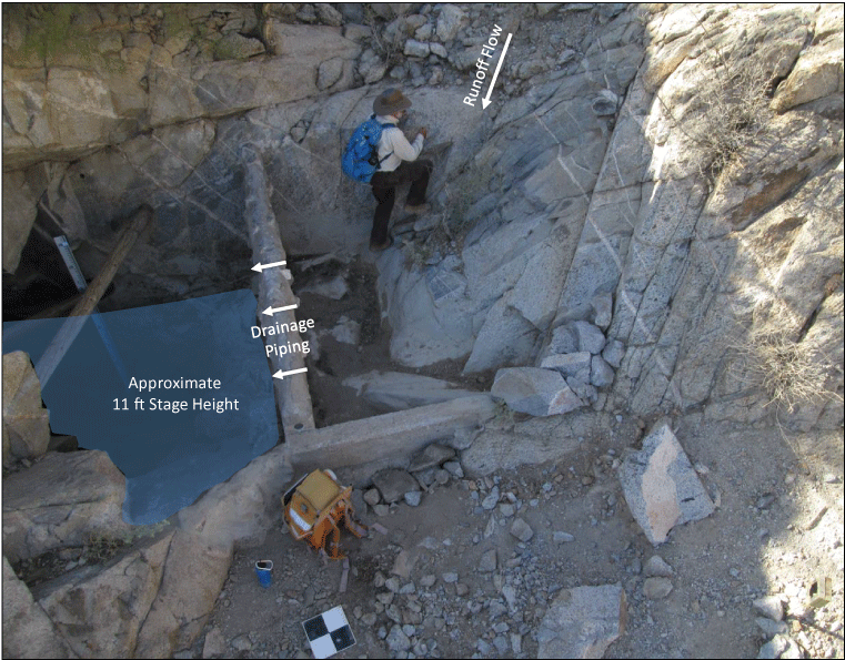
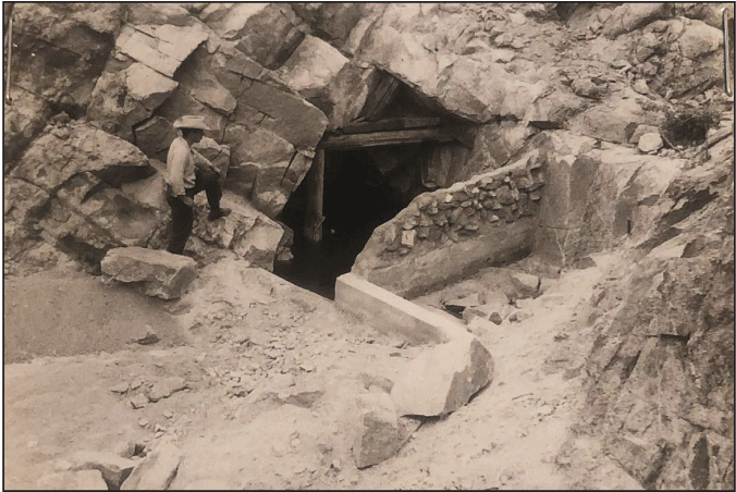
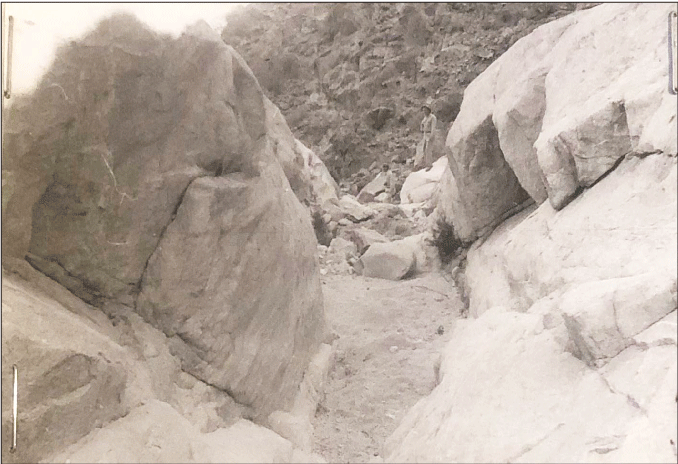
The entrance of Senita Tank in Cabeza Prieta National Wildlife Refuge (CPNWR), Arizona. A CPNWR employee, Shawn MacGill, climbs out of the upper runoff catchment that directs water towards the developed basin within bedrock through a series of drainpipes contained in the connecting wall. The previous capacity estimate of Broyles (1997; table 5) for Senita Tank best approximates the modeled 11-foot (ft) stage height that excludes the upper runoff catchment. Photograph by J. Caster, U.S. Geological Survey, February 15, 2022.
To achieve Objective 2, we built a stage-storage model for each tank using the ground-based lidar survey and the recently installed stage height rods. Stage-storage capacity below the maximum capacity had not been formally estimated with any other measurements prior to this study. Stage storage was predicted using a second-order polynomial equation for each tank that provided estimations within the 95-percent confidence interval bounds for all except the smallest stage heights at Senita Tank. For that tank, the stage-storage model equation in SNSgal underestimated storage capacity at a 1 ft height and slightly overestimated capacity up to a 4 ft stage height. Despite these differences, all three models provided an accurate estimate of stage-storage capacity from measured stage heights and will be useful tools for monitoring changes in water volumes for tank water storage and management needs.
We measured storage capacity after sediment was removed from each tank. Thus, the relationship between stage storage and stage height will change with future sedimentation. During pre-survey preparation, CPNWR staff removed sediment from each tank, with the greatest volume removed from Buckhorn Tank. In 1976, an estimated 5 yd3 (3.8 m3) of sediment was removed from Buckhorn (Dodson, 1976a). For both Buckhorn and Eagle Tanks, unconsolidated sediment had almost filled the channel to capacity behind the sediment retention dams located directly upstream of the tanks. Because little water can pool behind the dams and allow sediment to settle out, runoff water at these two tanks likely also contains sediment. A rock overhang above Eagle Tank causes runoff water to pool in an external basin separated from the excavated borehole by a short concrete wall containing several drainpipes, effectively serving as a secondary sediment retention basin and minimizing the amount of sediment deposited in the borehole. Using the stage-storage model, sediment filling the 1 ft stage height would reduce the maximum storage capacity by 4 percent, 1 percent, and 1 percent for Buckhorn, Senita, and Eagle Tanks, respectively. Sediment filling the 4 ft stage height would reduce the maximum fill capacity by 26 percent, 13 percent, and 14 percent for Buckhorn, Senita, and Eagle, respectively. Sediment over-topping the retention dam and filling Senita Tank is currently of low concern owing to the relatively large capacity remaining behind the dam, and the secondary sediment retention basin at Eagle Tank seems to minimize sedimentation. As supported by the quantity of sediment removed from Buckhorn Tank by CPNWR staff prior to surveying, however, sediment deposited by runoff water in this tank has the potential to greatly limit water storage capacity. For example, sedimentation since 2003 had limited the volume of Buckhorn Tank to about 50 percent of maximum capacity by July 2019. Refuge managers could use the estimates of sedimentation rates in this study (“Sediment Storage” section) to determine when and with what frequency to conduct periodic maintenance to clean the accumulated sediment out of the tanks to maximize water storage capacity.
The frequency with which floods contribute to sedimentation and tank recharge are not known. Broyles (1997) identified all three tanks as perennial water sources in the late 1990s, but CPNWR staff currently supplement this water supply by periodically hauling water to the tanks by truck and trailer. We do not yet have observations on changes in tank stage-storage volumes owing to factors like evaporation (appendix 1), leaks, or consumption by wildlife, but we expect that the natural fill volume and recharge rate for each tank is currently declining owing to decreases in precipitation and increases in air temperature in recent decades. Since 1970, annual rainfall has declined, and air temperatures have increased (fig. 12) using Sen’s Slope estimate of an assessment of precipitation and air temperature reported for the nearest National Oceanographic and Atmospheric Administration Cooperative Observer Program (NOAA–COOP) weather station Tacna 3 NE USC00028396 (NOAA, 2022), located approximately 30 miles north of Buckhorn Tank. The Sen’s Slope estimate is a non-parametric statistical test used to identify the magnitude and direction of temporal trends that is complemented by the Mann-Kendall test, used to assess the trend’s significance (Sen, 1968). Although winter rains have apparently not significantly changed over the last five decades since 1970, summer rains during the North American Monsoon have decreased at the 99 percent confidence interval (fig. 12). Additionally, temperatures within the region have significantly increased at the 99.9-percent confidence interval both annually and during the monsoon season (fig. 12). These climatic changes in rainfall patterns and temperatures may reduce natural water availability during seasonal periods when wildlife is more likely to visit tanks (Harris and others, 2020), thus increasing the importance of maintaining these resources.
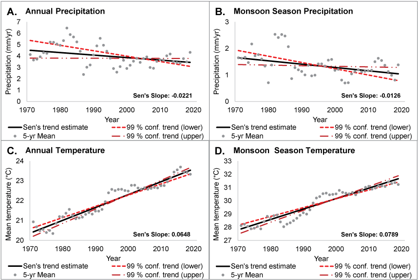
Graphs of fifty-year trends in precipitation and temperature at Tacna 3 NE National Oceanic and Atmospheric Administration Cooperative Observer Program station USC00028396 (National Oceanic and Atmospheric Administration, 2022), located approximately 30 miles north of Buckhorn Tank, Arizona. Mean annual (A), summer monsoon season (July–September) rainfall (B), mean annual (C), and summer monsoon season temperature (D) were summarized as 5-year (yr) moving window averages for the period from January 1, 1970, through December 31, 2021. Sen’s Slope (Sen, 1968) estimates are provided to indicate temporal trends and their significance, as determined by the Mann-Kendal trend test. The 99-percent (%) confidence interval trends are provided for reference, with the upper bounds representing the largest positive (or least negative) slope coefficient and the lower bounds representing the largest negative (or least positive) slope coefficient. In all cases, the upper and lower 99% confidence intervals were either both positive or both negative, indicating a significant temporal trend. For A and B, the trend estimate is significant at the 99% confidence interval. For C and D, the trend estimate is significant at the 99.9% confidence interval. mm/yr, millimeter per year.
Conclusion
In cooperation with the U.S. Fish and Wildlife Service (USFWS), the U.S. Geological Survey (USGS) Southwest Biological Science Center used ground-based lidar to measure the water storage capacity for three tanks in the Cabeza Prieta National Wildlife Refuge (CPNWR), Arizona, which are important water sources for desert bighorn sheep (Ovis canadensis mexicana). In addition to the maximum storage capacity, we also estimated storage capacity for at least six stage heights below the maximum capacity to develop a stage-storage model for each tank. The lidar surveys of each tank and estimated contours for each stage height are provided in an associated data release (Caster and others, 2024). Of the three tanks in this report, Buckhorn Tank had the largest maximum water storage capacity at 9,108.730 gallons (gal) (34,480.30 liters [L]), followed by Senita Tank at 8,623.308 gal (32,642.78 L), and then Eagle Tank at 6,039.603 gal (22,862.39 L). The resulting stage-storage models provide storage capacity estimates that are typically within the 95 percent confidence bounds of measured capacities and are accurate enough for refuge managers to monitor water volumes as needed. The ability to consistently monitor loss and recharge within these tanks is important for assessing water availability for desert bighorn sheep, though the accuracy of these estimates can change over time if sediment is deposited within the tanks and reduces water storage capacity. At Buckhorn Tank, a large volume of sediment was removed by CPNWR staff prior to the survey, demonstrating that sedimentation within the tank has occurred in the past and will likely occur in the future.
The confined and complex cave-like geometries of the tanks made ground-based lidar an invaluable tool for evaluating the three tanks within this report. Each tank had at least a portion of its storage confined within shallow boreholes within bedrock that were easily mapped by ground survey. Thus, we note the utility of ground-based lidar relative to, for example, airborne lidar which would not have adequately surveyed the interior of the borehole tanks but could be a different and additionally important resource to provide topographic and geomorphic context of the surrounding watersheds. These three tanks represented an immediate priority for water resource monitoring within the available time and budget of this project; however, these methods are applicable to other natural, modified, and developed water resources within the region. Development of storage capacity estimates, and stage-storage models from 3-dimensional ground-based lidar data, can be useful tools for understanding water storage, recharge, and loss in these habitats managed for desert wildlife.
References Cited
Broyles, B., 1997, Wildlife water-developments in southwestern Arizona: Journal of the Arizona-Nevada Academy of Science, v. 30, no. 1, p. 30–42, accessed October 3, 2023, https://www.jstor.org/stable/40022438.
Caster, J., Bransky, N., Sankey, J.B., Doerries, S., Sesnie, S., and Bedford, A., 2024, Data collected for estimation of storage capacity at managed water resources used by Desert Bighorn Sheep in Cabeza Prieta National Wildlife Refuge, Arizona, February 2022: U.S. Geological Survey data release, https://doi.org/10.5066/P9U6UYA0.
Caster, J., Sankey, J.B., Fairley, H., and Kasprak, A., 2022, Terrestrial lidar monitoring of the effects of Glen Canyon Dam operations on the geomorphic condition of archaeological sites in Grand Canyon National Park, 2010–2020: U.S. Geological Survey Open-File Report 2022–1097, 100 p., accessed October 3, 2023, at https://doi.org/10.3133/ofr20221097.
CloudCompare, 2019, CloudCompare, v. 2.10.2 [General Public License software]: CloudCompare, accessed October 3, 2023, at https://cloudcompare.org/.
Earth Resources Observation and Science (EROS) Center, 2018, USGS EROS Archive—Aerial Photography—National Agriculture Imagery Program (NAIP): U.S. Geological Survey web page, accessed October 3, 2023, at https://doi.org/10.5066/F7QN651G.
Fabbri, S., Sauro, F., Santagata, T., Rossi, G., and De Waele, J., 2017, High-resolution 3-D mapping using terrestrial laser scanning as a tool for geomorphological and speleogenetical studies in caves—An example from the Lessini mountains (North Italy): Geomorphology, v. 280, p. 16–29, accessed October 3, 2023. https://doi.org/10.1016/j.geomorph.2016.12.001.
Harris, G.M., Stewart, D.R., Brown, D., Johnson, L., Sanderson, J., Alvidrez, A., Waddell, T., and Thompson, R., 2020, Year-round water management for desert bighorn sheep corresponds with visits by predators not bighorn sheep: PLoS One, v. 15, no. 11, e0241131, accessed October 3, 2023. https://doi.org/10.1371/journal.pone.0241131.
National Oceanic and Atmospheric Administration (NOAA), 2022, USC00028396 TACNA 3 NE, AZ Weather Station: Climate Data Online, daily summary, accessed October 28, 2022, at https://www.ncdc.noaa.gov/cdo-web/datasets/GHCND/stations/GHCND:USC00028396/detail
Rydlund, P.H., Jr., and Densmore, B.K., 2012, Methods of practice and guidelines for using survey-grade global navigation satellite systems (GNSS) to establish vertical datum in the United States Geological Survey: U.S. Geological Survey Techniques and Methods, book 11, chap. D1, 102 p. with 44-p. app., accessed October 3, 2023, at https://doi.org/10.3133/tm11D1.
Seaber, P.R., Kapinos, F.P., and Knapp, G.L., 1987, Hydrologic Unit Maps: U.S. Geological Survey Water-Supply Paper 2294, 14 p., https://pubs.usgs.gov/publication/wsp2294.
Sen, P.K., 1968, Estimates of the regression coefficient based on Kendall’s tau: Journal of the American Statistical Association, v. 63, no. 324, p. 1379–1389, accessed October 3, 2023. https://doi.org/10.1080/01621459.1968.10480934.
U.S. Fish and Wildlife Service, [USFWS], 2006, Cabeza Prieta National Wildlife Refuge Comprehensive Conservation Plan, Wilderness Stewardship Plan and Environmental Impact Statement: Albuquerque, New Mex., U.S. Fish and Wildlife Service, Division of Planning, National Wildlife Refuge System, Southwest Region, 689 p., accessed October 3, 2023, at http://npshistory.com/publications/blm/el-camino-del-diablo/ccp-wsp-eis-2006.pdf.
Appendix 1. Observed and Modelled Relationships Between Stage and Water Storage Surface Area For Selected Tanks in Cabeza Prieta National Wildlife Refuge, Arizona
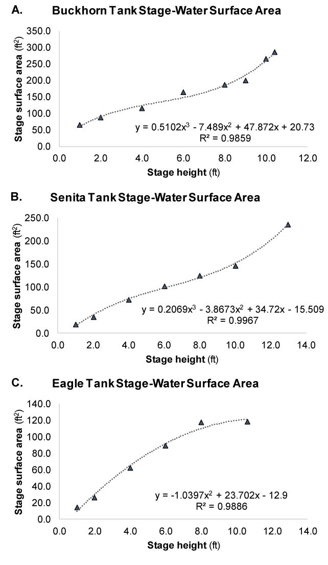
Graphs of observed and modelled relationships between stage surface area and stage height at Cabeza Prieta National Wildlife Refuge, Arizona for: Buckhorn Tank (A), Senita Tank (B), and Eagle Tank (C) for predicting water-storage surface area (y) in square feet (ft2) from stage height (x) in feet (ft). R2, coefficient of determination.
Appendix 2. Photographic Documentation of Buckhorn, Senita, and Eagle Tanks in Cabeza Prieta National Wildlife Refuge, Arizona
Buckhorn Tank
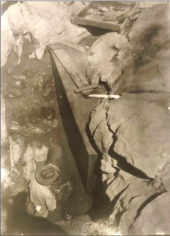
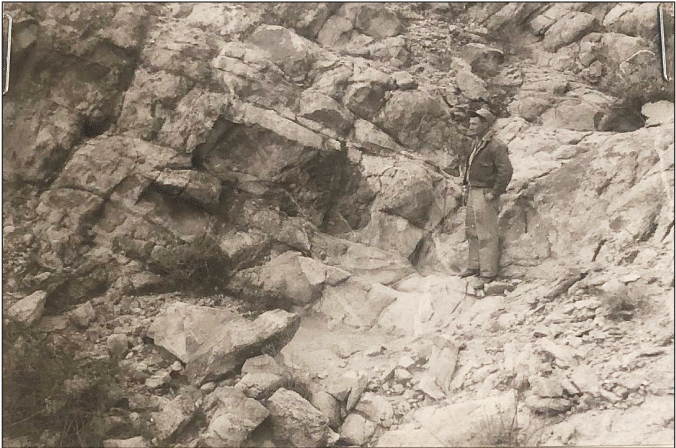
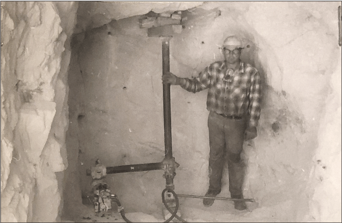
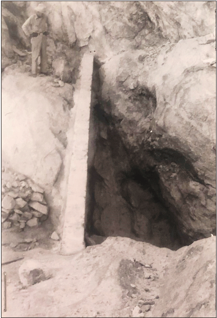
Photograph showing construction of Buckhorn Tank in the southern Cabeza Prieta Mountains, Cabeza Prieta National Wildlife Refuge, Arizona. The concrete liner (wall) was poured to seal off a rock fault and raise the pour point 2 feet. Approximate height may be judged in comparison with 5-foot-8-inch foreman Kempton (foreground). The masonry apron left of the wall provides access for wildlife. Immediately to the left of Kempton, an inclined shaft was tunneled 12 feet under an overhang (not shown) to give added depth and shaded water storage. All concrete was hand mixed in the mortar box shown in the top center. Photograph from U.S. Fish and Wildlife Service, 1950.
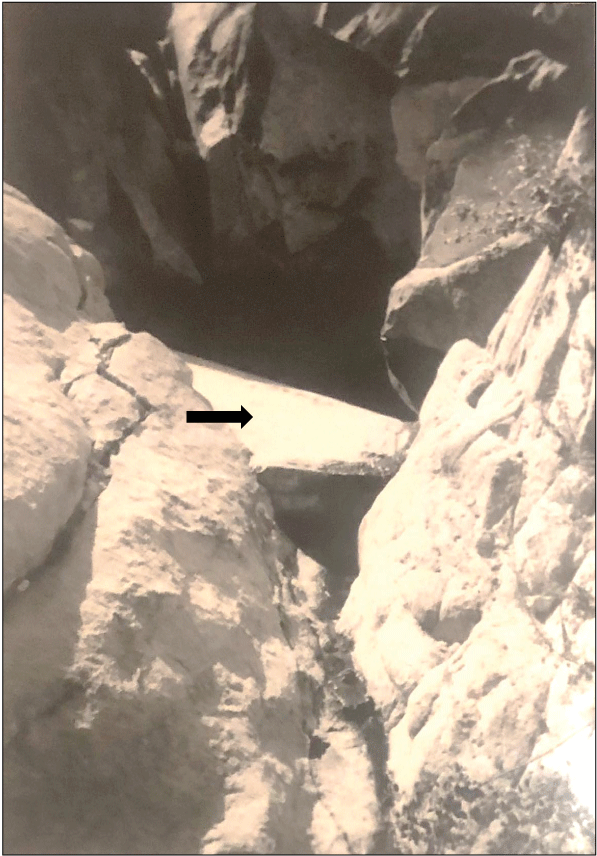
Photograph showing Buckhorn Tank full of water for the first time on October 5, 1949. Note the concrete liner (wall denoted with arrow) serving as the pour point for the tank, and the absence of the small masonry dam at the wall’s outer edge (closest to the photographer). Water is trickling out of the tank on the right side of the wall. The borehole is opposite the concrete wall, angling down and back towards the right. The reflection of part of the rock wall on the right is visible on the surface of the water. Photograph by Johnson, from U.S. Fish and Wildlife Service, 1950.
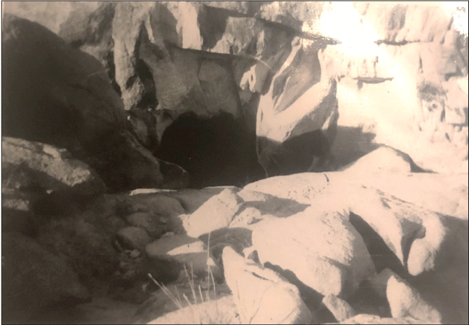
Photograph showing another view of Buckhorn Tank on October 5, 1949. The borehole is in the center of the photograph. Photograph by Johnson, from U.S. Fish and Wildlife Service, 1950.
Photograph of the borehole of Buckhorn Tank, completely cleaned of sediment, on February 14, 2022. Note the edge of the concrete liner in the foreground and the fixed rods in the background used to indicate stage height. Photograph by J. Sankey, U.S. Geological Survey.
Photograph showing Buckhorn Tank partially filled with damp sediment on June 9, 2020. Note the small masonry dam to the right of the concrete liner. This dam was constructed in 1976 to prevent sediment from backwashing into the tank (Dodson, 1976a), but it also elevated the pour point and lengthened the spillway, increasing the capacity of the tank. Photograph by S. MacGill, U.S. Fish and Wildlife Service.
Photograph showing Buckhorn Tank from above on February 14, 2022, completely cleaned of sediment. Note the fixed stage-height rod by the borehole, the outside edge of the concrete liner (at the right edge of the rock shadow), and the small masonry dam to the right (denoted with arrow). Photograph by S. Sesnie, U.S. Fish and Wildlife Service.
Photograph showing Buckhorn Tank full of water on July 24, 2019. Photograph by S. Doerries, U.S. Fish and Wildlife Service.
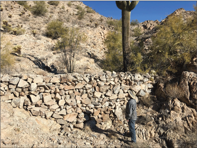
Photograph of the sediment retention dam, or sediment trap, and surrounding landscape on February 14, 2022. The dam is upstream from and above the tank, which is located just below the extent of the photograph. Alluvial (stream) sediment has built up behind the dam to the top of the structure. Note the small masonry dam (denoted with arrow) immediately downstream (below) from the sediment retention dam. For reference, 5-foot-7-inch U.S. Fish and Wildlife Service maintenance mechanic S. MacGill is center left. Photograph by J. Caster, U.S. Geological Survey.
Photograph showing a close-up view of the sediment retention dam upstream of Buckhorn Tank on July 24, 2019. Note the metal pipe at the bottom of the dam (partially obscured by the rock in front; denoted with arrow) installed during the initial construction in 1949. The broken, white 2-inch diameter polyvinyl pipe a couple feet above the metal pipe was installed in May 1976. Photograph by S. Doerries, U.S. Fish and Wildlife Service.
Photograph of the top of the sediment retention dam on February 14, 2022. Note the metal pipe extending through the bottom of the concrete dam (denoted with arrow), and the broken, white polyvinyl pipe a couple feet above. The sediment trap is full. Photograph by S. Sesnie, U.S. Fish and Wildlife Service.
Photograph of Buckhorn Tank with a water level 6 inches below maximum capacity on August 22, 2021. The small masonry dam, added in 1976, is in the foreground, and the borehole is on the back right side of the tank. Above the tank you can see the base of the sediment retention dam (top left) and the small, gray masonry dam (denoted with arrow) between the sediment retention dam and the tank itself. Photograph by D. Ebann, U.S. Fish and Wildlife Service.
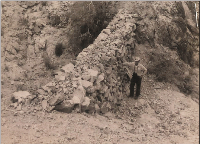
Photograph showing the sediment retention dam above Buckhorn Tank getting cleaned out on May 1–2, 1976. Members of the Arizona Desert Bighorn Sheep Society and other volunteers worked with Cabeza Prieta National Wildlife Refuge staff to remove silt that had accumulated upstream of the dam. The sediment trap was completely full, and material had been spilling over and into the tank for a number of years. Workers initially used shovels and a long bucket line to remove a few cubic yards of dry silt material by hand. Then they brought in hoses and a Gunnite pump to mechanically remove material. During the one-and-a-half-day project, an estimated 85 cubic yards of dry silt was removed from the trap. Even though workers dug down to the pipe at the bottom of the dam, the trap was not completely cleaned out. A couple feet above this metal pipe, they punched a 2-inch hole through the dam and inserted a polyvinyl pipe. The two pipes were covered with rock and sand to slow impaction by fine silt materials (Dodson, 1976a). Photograph by K. Voget, from U.S. Fish and Wildlife Service, 1977.
Photograph showing the sediment retention dam full of runoff water at Buckhorn Tank on February 6, 1958. Photograph by G. Monson, from U.S. Fish and Wildlife Service, 1958b.
Senita Tank
Photograph of the Senita Tank site in the Drift Hills, Cabeza Prieta National Wildlife Refuge, Arizona on December 26, 1957, prior to construction. Foreman Bob Russell looks the situation over. Photograph by G. Monson, from U.S. Fish and Wildlife Service, 1958b.
Photograph of the completed job at Senita Tank, including deflection device, on March 20, 1958. The tank had filled with water on February 6, 1958, prior to completion, precluding removal of debris from the borehole. Note the dry upper runoff catchment, or small silt trap catch basin, above the borehole, connected through a series of drainpipes through the concrete wall. Photograph from U.S. Fish and Wildlife Service, 1958b.
Photograph of the borehole of Senita Tank on February 15, 2022. Note the fixed rods used to indicate stage height up to 12 feet, although, it was extended to 14 feet after this photograph was taken. Upon evaluation of Senita Tank in 1960, the walls were noted to be heavily fractured, and it was determined that explosives had overshot and fractured the decomposed granite rock to a dangerous extent. In 1974, U.S. Fish and Wildlife Service personnel and volunteers from the Arizona Desert Bighorn Sheep Society removed large, loose boulders and at least 10 cubic yards of sand, silt, and rock, shoring up the borehole with wooden beams as they progressed. The tunnel was sealed using Thoroseal Plaster with Acryl 60 (Dodson, 1976b). Photograph by N. Bransky, U.S. Geological Survey.
Photograph of the Riegl VZ1000 laser scanner at the bottom of Senita Tank’s borehole, looking out towards the entrance. Note the drainpipes in the concrete wall dividing the borehole from the upper runoff catchment. Photograph by J. Caster, U.S. Geological Survey, February 15, 2023.
Photograph of the entrance to Senita Tank on February 15, 2022, taken from downstream. A concrete wall perforated with drainpipes separates the borehole on the left from the upper runoff catchment on the right. Note the small masonry dam at the mouth of the borehole, on the left side of the perforated concrete wall; it was constructed in 1974 by U.S. Fish and Wildlife Service personnel and Arizona Desert Bighorn Sheep Society volunteers to increase storage capacity and prevent silt from backflowing into the tank. The upper runoff catchment was cleaned out and sealed in 1976, as was the small masonry dam (Dodson, 1976b). The top of the sediment retention dam can be seen above and slightly right of the upper runoff catchment. For reference, 5-foot-7-inch U.S. Fish and Wildlife Service maintenance mechanic S. MacGill is in the left foreground. Photograph by J. Sankey, U.S. Geological Survey.
Photograph of the entrance to Senita Tank on February 15, 2022. Note the drainpipes at the bottom of the concrete wall separating the upper runoff catchment (front) from the borehole (back). Photograph by J. Caster, U.S. Geological Survey.
Photograph viewing the entrance to Senita Tank on February 15, 2022, taken from upstream. Photograph by N. Bransky, U.S. Geological Survey.
Photograph of the completed sediment retention dam at Senita Tank on March 20, 1958. An unnamed worker is standing on the downstream side of the dam. Photograph from U.S. Fish and Wildlife Service, 1958b.
Photograph of the downstream side of the sediment retention dam at Senita Tank on February 15, 2022. Physical scientist Ashton Bedford (U.S. Geological Survey; approximately five-foot-ten-inches) stands below the structure for scale. Photograph by J. Sankey, U.S. Geological Survey.
Photograph of the sediment retention dam at Senita Tank on February 15, 2022. Note the accumulated sediment upstream (left) of the dam and a 1.9-meter (6.2-foot) survey tripod on top of the dam for scale. Photograph by J. Caster, U.S. Geological Survey.
Eagle Tank
Photograph of the Eagle Tank site in the Sierra Pinta, Cabeza Prieta National Wildlife Refuge, Arizona on November 6, 1957, before construction began. The tank was blasted out in the middle of the bottom of the photo, and the dam site is at the upper left. Photograph by G. Monson, from U.S. Fish and Wildlife Service, 1958a.
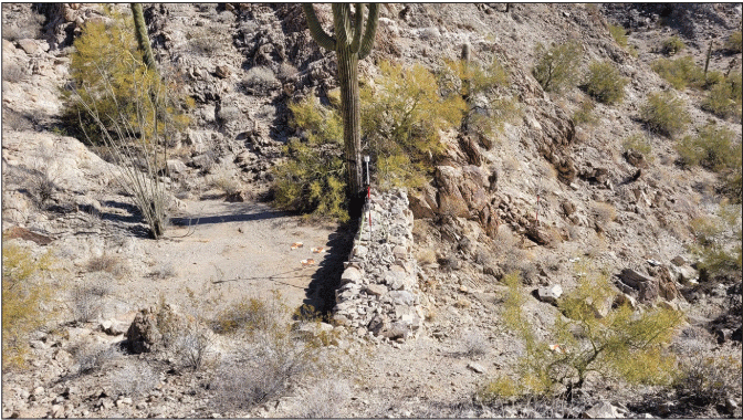
Photograph of the Eagle Tank site on February 16, 2022. Note the sediment retention dam slightly above center and the borehole below. Photograph by S. Sesnie, U.S. Fish and Wildlife Service.
Photograph showing the inside of the “hole” at Eagle Tank on November 25, 1957, during construction. Air tool operator Best stands by apparatus used to hold compressed air rock drill while it bores holes to hold the dynamite. Photograph by G. Monson, from U.S. Fish and Wildlife Service, 1958a.
Photograph of the site of the sediment retention dam at Eagle Tank on November 6, 1957, before construction, looking downstream. The sand in the foreground was used to build the concrete dam. Photograph by G. Monson (U.S. Fish and Wildlife Service, 1958a).
Photograph of the sediment retention dam at Eagle Tank on December 11, 1957, beginning to take shape. Workers build the forms for the dam and move sand immediately downstream of the dam for mixing concrete. Photograph by G. Monson, from U.S. Fish and Wildlife Service, 1958a.
Photograph showing the sediment retention dam being poured on December 18, 1957. Note the access trail to dam at left and workers mixing concrete below the dam. Photograph by Duncan, from U.S. Fish and Wildlife Service, 1958a.
Photograph of the completed sediment retention dam on January 23, 1958, 11 feet high by 23 feet long. A metal pipe at the bottom of the dam allows water to flow downstream into the tank, even after the dam filled with rock and silt. Photograph by G. Monson, from U.S. Fish and Wildlife Service, 1958a.
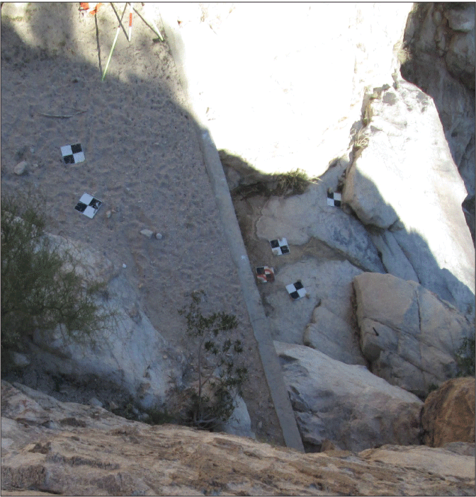
Photograph of the sediment retention dam on February 17, 2022. Sediment accumulation behind the dam covers the bedrock and gravel upstream of the dam that is visible in figure 2.30. The 1-foot (0.3-meter) square photo panels were used for scale. Photograph by J. Caster, U.S. Geological Survey.
Photographic documentation of sediment accumulated up to the top of Eagle Tank’s sediment retention dam on February 17, 2022 (looking downstream). Photograph by S. Sesnie, U.S. Fish and Wildlife Service.
Photograph showing the borehole and secondary sediment retention basin at Eagle Tank on February 17, 2022. The secondary sediment retention basin is the shallow basin enclosed by short concrete walls and the rock walls of the canyon just outside of the borehole. The concrete wall separating this basin from the borehole contains numerous drainpipes, which allows water to flow from the basin into the borehole. The overhang above the borehole causes fast-moving water with sediment to pool in the external basin, minimizing the amount of sediment deposited in the borehole. The black deposits on the rock above the borehole indicate the flow of water into the borehole and basin. Photograph by S. Sesnie, U.S. Fish and Wildlife Service.
Photograph of the borehole of Eagle Tank on February 17, 2022. Note the fixed rods used for determining stage height up to 12 feet. Photograph by S. Sesnie, U.S. Fish and Wildlife Service.
References Cited
Seaber, P.R., Kapinos, F.P., and Knapp, G.L., 1987, Hydrologic Unit Maps: U.S. Geological Survey Water-Supply Paper 2294, 14 p., https://pubs.usgs.gov/publication/wsp2294.
Conversion Factors
U.S. customary units to International System of Units
International System of Units to U.S. customary units
Temperature in degrees Celsius (°C) may be converted to degrees Fahrenheit (°F) as follows:
°F = (1.8 × °C) + 32.
Temperature in degrees Fahrenheit (°F) may be converted to degrees Celsius (°C) as follows:
°C = (°F – 32) / 1.8.
Datums
Vertical coordinate information is referenced to the North American Vertical Datum of 1988 (NAVD 88) and used the geoid model Geoid18.
Horizontal coordinate information is referenced to the 2011 adjustment of the North American Datum of 1983 NAD 83 (2011) and used the cartesian coordinate system: Universal Transverse Mercator (UTM) zone 12N.
Abbreviations
CCP
Comprehensive Conservation Plan
CI
confidence interval
CPNWR
Cabeza Prieta National Wildlife Refuge
DEM
digital elevation model
GNSS
Global Navigation Satellite Systems
GPS
global positioning system
lidar
light detection and ranging
NAD 83
North American Datum of 1983
NAIP
National Agricultural Imagery Program
NAVD 88
North American Vertical Datum of 1988
NGS
National Geodetic Survey
NHD
National Hydrography Dataset
NOAA–COOP
National Oceanographic and Atmospheric Administration Cooperative Observer Program
NSRS
National Spatial Reference System
OPUS
Online Positioning User Service
QRP
Quick Response Program
RMSE
root mean square error
RTK
real-time kinematic
SE
standard error
TIN
triangulated irregular network
UTM
Universal Transverse Mercator
USDA
U.S. Department of Agriculture
USFWS
U.S. Fish and Wildlife Service
USGS
U.S. Geological Survey
Disclaimers
Any use of trade, firm, or product names is for descriptive purposes only and does not imply endorsement by the U.S. Government.
Although this information product, for the most part, is in the public domain, it also may contain copyrighted materials as noted in the text. Permission to reproduce copyrighted items must be secured from the copyright owner.
Suggested Citation
Sankey, J.B., Caster, J., Bransky, N., Fuest, S., Sesnie, S., and Bedford, A., 2024, Lidar estimation of storage capacity for managed water resources used by desert bighorn sheep (Ovis canadensis mexicana) at Cabeza Prieta National Wildlife Refuge, Arizona: U.S. Geological Survey Open-File Report 2024–1046, 51 p., https://doi.org/10.3133/ofr20241046.
ISSN: 2331-1258 (online)
Study Area
| Publication type | Report |
|---|---|
| Publication Subtype | USGS Numbered Series |
| Title | Lidar estimation of storage capacity for managed water resources used by Desert Bighorn Sheep (Ovis canadensis mexicana) at Cabeza Prieta National Wildlife Refuge, Arizona |
| Series title | Open-File Report |
| Series number | 2024-1046 |
| DOI | 10.3133/ofr20241046 |
| Publication Date | October 22, 2024 |
| Year Published | 2024 |
| Language | English |
| Publisher | U.S. Geological Survey |
| Publisher location | Reston, VA |
| Contributing office(s) | Southwest Biological Science Center |
| Description | Report: viii, 51 p.; Data Release |
| Country | United States |
| State | Arizona |
| Other Geospatial | Cabeza Prieta National Wildlife Refuge |
| Online Only (Y/N) | Y |