

Numerical Modeling of Circulation and Wave Dynamics Along the Shoreline of Shinnecock Indian Nation in Long Island, New York
Links
- Document: Report (3.53 MB pdf) , HTML , XML
- Data Release: USGS Data Release - Three-dimensional point cloud data collected with a scanning total station on the western shoreline of the Shinnecock Nation Tribal lands, Suffolk County, New York, 2022
- NGMDB Index Page: National Geologic Map Database Index Page (html)
- Download citation as: RIS | Dublin Core
Acknowledgments
This report was prepared as a part of a multiple year project funded by the National Fish and Wildlife Foundation (project number 55032) to collect physical and ecological data and to conduct numerical modeling of living shoreline restoration projects to assess the effectiveness of living shoreline structures across the northeast and mid-Atlantic coasts. This study was conducted in collaboration with Northeastern University. We thank Drs. Lihwa Lin and Gangfeng Ma for their constructive reviews of this report.
Abstract
The Shinnecock Indian Nation on Long Island, New York, faces challenges of shoreline retreat, saltwater intrusion, and flooding of the Tribal lands under changing climate and rising sea level. However, understanding of the dynamics of tidal circulation and waves and their impacts on the Shinnecock Indian Nation’s shoreline remains limited. This numerical study employs the integrated modeling capabilities of the hydrodynamic model Delft3D-FLOW and the spectral-wave model Simulating WAves Nearshore (SWAN) to investigate the circulation and wave dynamics along the shoreline of Shinnecock Indian Nation. The results of the 1-year long simulation indicate the majority of wind waves approach the Shinnecock Nation shorelines at normal wave angles, with yearly averaged offshore wave height of around 0.2 meter, maximum wave height reaching 0.65 meter, and yearly averaged offshore wave power of approximately 50 watts per meter. Boulders, acting as natural barriers, have been placed along the shoreline to reduce erosive wave forcing. Simulation results indicate the boulders to the north end effectively attenuate wave energy and reduce annual wave power, while the boulders near the two tidal ponds adjacent to the Tribal cemetery only have a slight influence on wave energy. There are large spatial variabilities in wave attenuation and current velocity reduction by the boulders. The model framework developed in this study can be utilized for the optimal design of nature-based solutions, guiding decisions on the placement of living shoreline structures and determining their optimal size. This study further identifies data and knowledge gaps as well as future research opportunities that can enhance the performance of numerical models and contribute to the scientific understanding of coastal processes and facilitate the optimal design of hybrid living shorelines in the future to achieve the maximum protective efficacy. This research can help to inform strategies for safeguarding vulnerable coastal communities and promoting resilience and sustainability of shoreline along the Shinnecock Indian Nation.
Introduction
In the last two decades, living shorelines became increasingly popular for coastal restoration and protection against shoreline retreat and habitat loss (Sutton-Grier and others, 2015; O’Donnell, 2017). Living shorelines use artificial oyster reefs, such as oyster castles or oyster shells, and vegetation, such as salt marshes and seagrass, to reduce sediment erosion and habitat loss. Sometimes hybrid approaches that combine “green” and “grey” structures (for example, salt marsh bands with rock breakwater and large boulders) are also used. Following Hurricane Sandy (2012), the U.S. Congress designated funds to restore shorelines and many living shoreline projects with varying building materials and with different configurations (for example, distance from shore, length, and structure gaps) were constructed along the New England and mid-Atlantic coasts in 2013. Nevertheless, the efficacy of these living shoreline structures in protecting shorelines from erosion is limited, thus preventing the design and implementation of optimal solutions to achieve sustainable engineering and ecological benefits. Since 2017, U.S. Geological Survey (USGS) scientists have worked with collaborators from Northeastern University, U.S. Fish and Wildlife Service, Louisiana State University, The Nature Conservancy, and other State and local agencies to conduct monitoring and modeling of wind waves, current patterns, and sediment dynamics of the living shoreline restoration projects with funding from the National Fish and Wildlife Foundation Hurricane Sandy Coastal Resiliency Competitive Grant Program. Four living shoreline restoration projects (Gandys Beach, New Jersey; Chincoteague, Virginia; Fog Point, Maryland; and Shinnecock, New York) were selected from 12 restoration projects along the New England and mid-Atlantic coasts (Wang and others, 2021, 2023, 2024).
It is recognized that wind waves are one of the major driving forces of shoreline erosion (for example, Marani and others, 2011). Therefore, the main goal of living shoreline structures is to reduce wave and current energy and allow sediment to be delivered to shore and connected tidal wetlands. Previous studies found that living shoreline structures are effective in wave attenuation and erosion reduction as well as in promoting sediment deposition under certain wind, wave, and tidal conditions, but may not be effective in other conditions such as high-wave-induced and surge-induced overtopping, large tidal ranges, and deep water depth (Wiberg and others, 2019; Zhu and others, 2020; Morris and others, 2021; Wang and others, 2023, 2024). Examining the current and wave dynamics with and without living shoreline structures can help to determine if structures are effective in shoreline protection against wave-induced erosion. If existing structures are not effective, designing and implementing new and optimal structures may be necessary.
The Shinnecock Indian Nation is located along the eastern Shinnecock Bay in Long Island, New York. The Tribe’s territory is particularly vulnerable to storms and associated flooding, especially after Hurricane Sandy’s (2012) storm surge breached the barrier beach. Following Hurricane Sandy, the shoreline was highly degraded, rendering it especially susceptible to sea level rise and potential impacts of future storms. Faced with challenges associated with beach erosion, shoreline retreat, flooding, water quality decline, and degradation of fish and wildlife habitat, the Shinnecock Indian Nation, in conjunction with Federal, State, and local agencies, initiated the Coastal Habitat Restoration Project in 2015 (Anchor QEA, LLC, The Nature Conservancy, and Fine Arts and Sciences, LLC, 2019). The project aims to restore and strengthen natural system resilience, enhance ecological diversity along the shoreline, and improve tidal flushing in the two tidal ponds to reduce the mosquito population. A strategically designed hybrid living shoreline, incorporating features like constructed oyster reefs and headland bay beaches with vegetation, could provide the necessary structural stability to attenuate wave energy, maintain a stable shoreline, and provide ecosystem services such as food production, nutrient removal, and water quality improvement (National Oceanic and Atmospheric Administration [NOAA], 2015). This multistage restoration effort involves (1) dredging around 30,000 cubic yards of sand from a nearby canal to replenish the beach; (2) installing sand fences and planting coastal marshes to stabilize the sand; and (3) placing heavy boulders along the 3,000 feet of shoreline to provide additional protection against energetic incoming waves. The success of resilient hybrid living shoreline solutions relies on a comprehensive understanding of wave climate, influenced by factors such as wind fetch, wind intensity and duration, bed elevations, and geographical conditions (Vona and others, 2021).
Numerical modeling is an important tool for assessing the effectiveness of existing living shoreline structures, exploring optimal design of living shoreline structures, and predicting the effects of the living shoreline structures on current, wave, and sediment dynamics and the responses of shoreline and associated tidal wetland morphology under various storms conditions (Vona and others, 2021; Huff and others, 2022; Salatin and others, 2022; Zhu and others, 2023). Numerical efforts have been devoted to Shinnecock Inlet and Shinnecock Bay (for example, Militello and Kraus, 2001; Buonaiuto and Militello, 2003; Demirbilek and others, 2008; Ahn and Ronan, 2019; Lin and others, 2022). Among them, Militello and Kraus (2001) carried out numerical simulations to identify and evaluate potential consequences of mining the flood-tidal shoal at Shinnecock Inlet for material to be placed on the ocean-fronting beach adjacent to a jetty to the west of the inlet. The hydrodynamic model ADvanced CIRCulation (ADCIRC; Luettich and others, 1992) was used to simulate water levels and currents, while the wave model STeady WAVE (STWAVE; Resio, 1987; Smith and others, 1999) was employed to simulate wave transformation and refraction properties. Lin and others (2022) developed a numerical sediment transport model using Coastal Modeling System (Sanchez and others, 2014) to explore engineering solutions for the sand borrow area and structural alternatives to mitigate the down-drift beach erosion at Shinnecock Inlet. Their modeling results revealed that a partial ebb shoal borrow area design without structural alternatives performed better together with the down-drift beach nourishment applications.
Numerical models focusing specifically on the Shinnecock Indian Nation shoreline are currently unavailable. Specifically, there are no data or information that can used to determine the tidal current and wave dynamics with and without living shoreline structures or to assess the effectiveness of the structures on shoreline protection and restoration. The limited existing data and knowledge gaps regarding the wave environment along the Shinnecock Indian Nation shoreline pose challenges in designing and evaluating the effectiveness of these nature-based mechanisms in stabilizing and retaining sand. The extent that boulders reduce wave energy and the efficacy of these natural mechanisms remain uncertain. This study is the first attempt to simulate tidal current and wave dynamics and to investigate the impact of strategically placed boulders on wave attenuation and current velocity along the Shinnecock Indian Nation shoreline using the coupled hydrodynamic model Delft3D-FLOW (Deltares, 2022) and the spectral-wave model Simulating WAves Nearshore (SWAN; Booij and others, 1999) models. The objectives of this study are to (1) simulate the hydrodynamics and wave climate within Shinnecock Bay near the Shinnecock Indian Nation; (2) quantify the effects of the placement of boulders on current velocity and wave energy dissipation; (3) identify critical data and knowledge gaps for improving numerical models for the Shinnecock Indian Nation shoreline; and (4) provide guidance for field measurements in support of shoreline protection and restoration. The modeling tool and simulation results can help the Shinnecock Indian Nation design and implement optimal living shoreline structures to achieve long-term engineering benefit of shoreline protection against wave-induced beach erosion and shoreline retreat.
Study Area
The Shinnecock Indian Nation, situated on the eastern shore of Shinnecock Bay in Long Island, adjacent to Southampton, New York (fig. 1), comprises 800 acres. The tidal range in Shinnecock Inlet (fig. 1) is approximately 0.99 meter (m) (https://www.tidespro.com/). The majority of the Shinnecock Indian Nation situates on a low-lying, south-facing peninsula along Shinnecock Bay (Shinnecock Indian Nation, 2013). The shoreline is characterized by its unique geographical features and cultural significance. Owing to storms, the two tidal ponds next to the Shinnecock Indian Nation Cemetery (fig. 2) have turned into stagnant bodies of water where mosquito larvae thrive. During Winter Storm Elliott in 2022, the Shinnecock Indian Cemetery and the adjacent tidal ponds experienced major flooding, attributed to a combination of high astronomical tides and winds out of the south and southwest, which pushed seawater to the northeast side of Shinnecock Bay. Inundation will likely become increasingly common due to sea level rise and observed increases in storm frequency and intensity (Hague and others, 2020). The location of the two tidal ponds exposed the cemetery to flood inundation on three sides. Cuffee Beach, located along the western-facing shoreline of Shinnecock Bay (fig. 1), has experienced shoreline retreat and coastal erosion. North of Cuffee Beach there is a dynamic coastal area where an extended spit forms a significant embayment and estuarine habitat area. This area is susceptible to ongoing transformations due to variations in sediment transport, overtopping, erosion, overwash, and reformation of the coastal spit. Such transformation can result in transitions of the ecological features of the area, affecting the habitat suitability for fish and wildlife species (Shinnecock Indian Nation, 2013). In addition, there are residences situated directly landward of the coastal embayment. Changes to the embayment region such as a loss of the coastal spit can result in an increase in wave energy and coastal flood inundation of the landward areas.
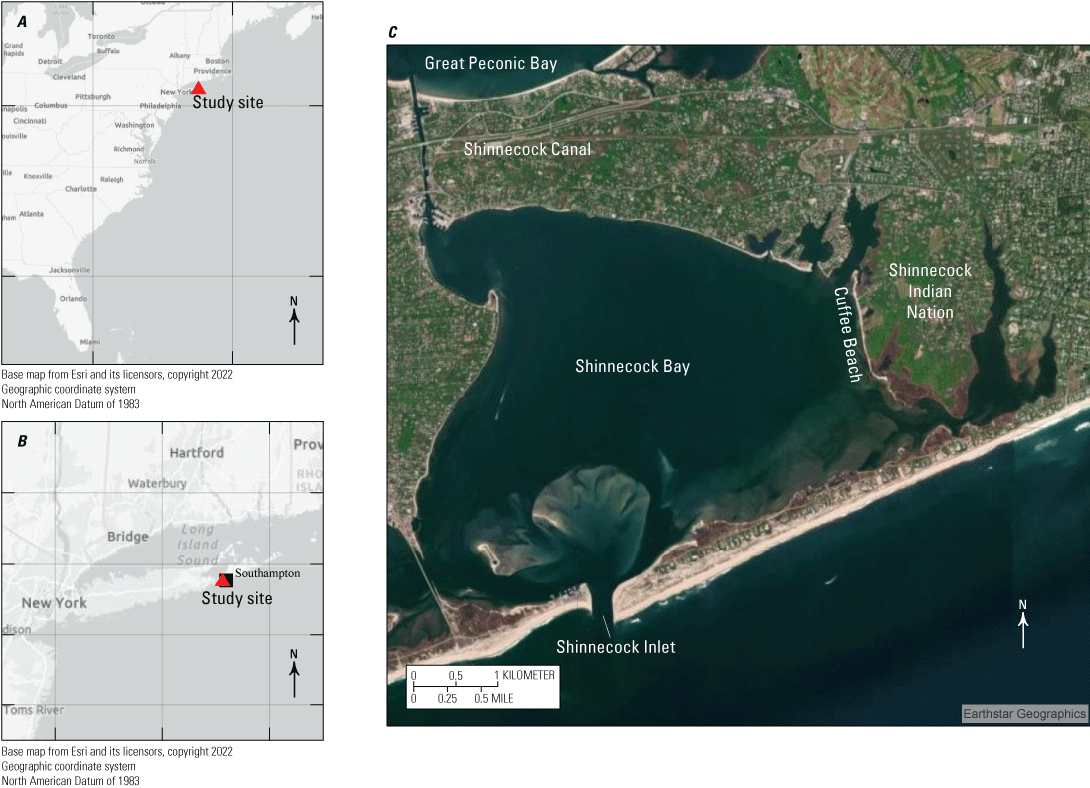
A, Study site (red triangle) relative to the east coast of the United States; B, study site (red triangle) relative to Long Island, New York; and C, Shinnecock Indian Nation relative to Shinnecock Bay.
The Shinnecock Indian Nation, in cooperation with Cornell Cooperative Extension, used living shoreline approaches to restore the shoreline along the eastern Shinnecock Bay. The living shoreline restoration efforts along the Shinnecock Indian Nation shoreline include placement of boulders, oyster cages, or shells; replenishing of sand; and planting of salt marsh and seagrass. The major structures constructed along the shore are the boulders (fig. 2) that are expected to alleviate wave-induced shoreline erosion. Figure 3 presents the boulder crest elevations from a light detection and ranging (lidar) survey and boulder heights computed relative to the bed elevation. The mean boulder height is 0.79 m with a standard deviation of 0.22 m. A total of 9,280 boulders were identified in the lidar survey, resulting in an estimated population density of 12.85 boulders per square meter (boulders/m2). The average boulder width is approximated as 0.5 m according to Google Earth data. The field survey of boulder locations and crest elevations was conducted by USGS New York Water Science Center in 2022 (figs. 2D, 3, Capurso and others, 2024). The sand characteristics at the study site have not been surveyed; however, data from usSEABED (https://cmgds.marine.usgs.gov/usseabed/) indicate that the central region of the Shinnecock Bay is predominantly composed of cohesive sediment. This composition raises concerns regarding potential settlement or scattering of boulders. Continuous monitoring of boulder locations and crest elevations can provide information on how the site is changing over time.
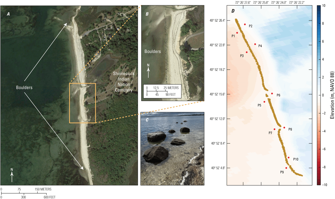
A, Overview of the boulder layout; B, zoom-in of the boulder layout near Shinnecock Indian Nation Cemetery; C, photograph of boulders near the cemetery (photograph taken in August 2022 by Qin Chen, Northeastern University, used with permission); and D, numerical output stations (P1–P10, red dots) around boulders (brown dots).
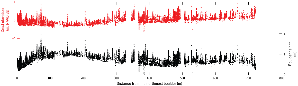
Boulder crest elevations and boulder heights. NAVD 88, North American Vertical Datum of 1988; m, meter (source: U.S. Geological Survey New York Water Science Center).
Methods
Open-sourced hydrodynamic model Delft3D-FLOW (Deltares, 2023) and spectral wave model SWAN are employed and coupled to simulate the flow and wave fields in Shinnecock Bay with a focus on the Shinnecock Indian Nation shorelines. In this study, Delft3D-FLOW operates in its horizontal two-dimensional mode to solve the depth-averaged flow equation for water level (η) and depth-averaged current (U). The depth-averaged flow model is sufficient for well-mixed shallow estuaries, such as Shinnecock Bay. Moreover, SWAN only takes depth-averaged currents as the inputs. SWAN solves the spectral wave action balance equation for wave spectra and integrated wave parameters, including significant wave height (Hs), peak wave period (Tp), and peak wave direction (θp). The study period spans the year 2018, a year notable for the occurrence of four nor'easters affecting the east coast of the United States (Zhu and others, 2020). Additionally, Wang and others (2022) found that the wind conditions observed in 2018 are representative of the broader climatic patterns in 2015, 2016, 2019, and 2020. The modeling system developed in this study can serve as a tool for simulating and analyzing the impacts of major tropical storms and hurricanes. Future studies may utilize this system to better understand the dynamics of extreme weather events and the effectiveness of boulders on shoreline protection.
Mesh Development and Topobathy
This study uses a nesting approach that features three levels of computational domains, each discretized with curvilinear meshes. The level 1 ocean-scale domain (L1) spans part of the north Atlantic Ocean, Gulf of Mexico, and Caribbean Sea. While the L1 mesh structure aligns with that of Zhu and others (2023), modifications have been made to refine the mesh specifically at Shinnecock Bay. The level 2 bay-scale domain (L2) (depicted by the green box in fig. 4) encompasses the entire Shinnecock Bay, measuring approximately 24,488 m alongshore and 10,158 m cross shore. Its south boundary extends approximately 4,400 m into the Atlantic Ocean, with a water depth of around 26 m. The north boundary predominantly lies on land but traverses Cold Spring Pond adjacent to Great Peconic Bay and the Shinnecock Canal connecting Shinnecock Bay and Great Peconic Bay. The level 3 local scale domain (L3) (indicated by the blue box in fig. 4) covers the Shinnecock Indian Nation and the eastern part of Shinnecock Bay. Overall, the mesh sizes gradually decrease from 40 kilometers in deep basins and flat shelves (L1) to around 1 m at the study site (L3). Table 1 lists the mesh size ranges within the three levels of computational domains.
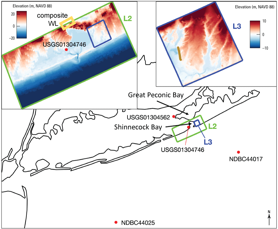
Study site relative to Long Island, New York, U.S. Geological Survey (USGS) tide stations (USGS, 2024a, b), and National Data Buoy Center (NDBC) wave buoys (red dots). The green box and blue box outline the level 2 (L2) and level 3 (L3) computational domains, respectively. Left inset: elevation map of the L2 domain. Red dot represents a tide station. A composite water level (WL) condition is imposed to the north boundary (yellow box) of the L2 domain. Right inset: elevation map of the L3 domain and locations of boulders (brown line). NAVD 88, North American Vertical Datum of 1988; m, meter.
Topographic and bathymetric data are obtained from multiple sources: (1) the northeast Atlantic 3 arc-second digital elevation models (DEMs) with about 90 m horizontal resolutions (NOAA National Geophysical Data Center, 1999); (2) NOAA and Federal Emergency Management Agency (FEMA) bathymetry data with horizontal resolutions ranging from 30 to 2 m (FEMA, 2014); and (3) USGS Coastal National Elevation Database topobathy DEM compiled in 2016 with 1 m resolution based on lidar data for topography and 10 m resolution for bathymetry (Danielson and others, 2016).
Model Coupling, Boundary Conditions, and Meteorological Forcing
Delft3D-FLOW and SWAN are one-way coupled to optimize computational efficiency. The spatial-temporal varying water levels and depth-averaged current fields from the Delft3D-FLOW model feed into SWAN for wave simulations; however, the wave fields from SWAN are not sent back to the FLOW model for flow simulations. While in deep waters, the flow fields are less affected by waves; in the surf zone, they are more subject to the influence of wave actions because of (1) enhanced vertical mixing processes attributed to turbulence generated by white capping and depth-limited wave breaking; (2) increased weight of wave-induced bottom shear stress; and (3) wave setup/setdown induced by the gradient of radiation stress. In the nearshore, Zhu and others (2023) demonstrated that two-way coupling slightly outperforms one-way coupling in water level and wave simulations. Moreover, running L3 Delft3D-FLOW for the whole year is computationally demanding; therefore, we use water levels from L2 Delft3D-FLOW as input to L3 Delft3D-WAVE. Given that the effects of boulders on water levels and depth-averaged current fields are not validated due to the lack of field data, the current fields are not activated in L3-WAVE.
At the seaward boundary of the L1 domain, the Delft3D-FLOW model is forced with the astronomical tide with seven principal constituents determined from a tidal constituent database (Mukai and others, 2002). In SWAN, integral wave parameters (that is, Hs, Tp, and θp) from the global and regional scale wave model (WW3 model) are enforced along the seaward boundary to ensure that long wave signals are included in L1 to L3 SWAN models (Zhu and others, 2023). The Delft3D-FLOW and SWAN models in the upper-level domain provide boundary conditions, including hourly outputs of water level, current, and wave spectra, for the lower-level or nested domain.
The north boundary of the L2 domain intersects the Shinnecock Canal, an artificially cut and maintained conveyance channel that allows water to flow from Great Peconic Bay to Shinnecock Bay (fig. 1). A gate that prohibits water from flowing in the opposite direction is operated based on the disparity in water levels between Great Peconic Bay and Shinnecock Bay. Water levels are monitored at the USGS stations in Great Peconic Bay (USGS01304562; USGS, 2024a) and Shinnecock Bay (USGS01304746; USGS, 2024b), as depicted in figure 5 (refer to figure 4 for station locations). Due to the difference in tidal phases between the two bays, high tide and low tide events occur at distinct times on each end of the canal. The peak highs in Shinnecock Bay lead the peak highs in Great Peconic Bay by around 5 hours (see upper panel in fig. 5). In Shinnecock Bay, high and low tide stages correspond with rising and falling tides, respectively, in Great Peconic Bay. Conversely, in Great Peconic Bay, high and low tide stages correspond to falling and rising tides, respectively, in Shinnecock Bay. The gate opens when the water levels in Great Peconic Bay surpass those in Shinnecock Bay and closes when the water levels in the two bays are nearly equal. Representative values for the water level difference are 30 and −5 centimeters for gate opening and closing, respectively (Militello and Kraus, 2001). To simulate the timing and one-way flow through the Shinnecock Canal, a composite water level boundary condition, computed as the maximum water levels at two ends of the canal (blue line in fig. 5), is implemented at the north boundary of the L2-FLOW model.
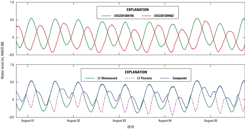
Upper panel: Water level measurements at U.S. Geological Survey (USGS) stations USGS01304562 (USGS, 2024a) in Great Peconic Bay and USGS01304746 (USGS, 2024b) in Shinnecock Bay during the first few days of August 2018. Lower panel: Modeled water levels from level-1 Delft3D-FLOW at two ends of the canal and composite water levels during the first few days of August 2018. NAVD 88, North American Vertical Datum of 1988; m, meter.
The U.S. Army Corps of Engineers Engineering Research and Development Center’s Coastal and Hydraulics Laboratory deployed a current meter in the Shinnecock Canal in 1998 to monitor the current speed in the canal (Militello and Kraus, 2001). In this study, we locally increased the bottom friction factor (ƒ0) from 0.02 to 0.04 to align the modeled maximum current speed with the field measurements. Figure 6 displays the depth-averaged velocity from L2-FLOW without composite water level conditions and with composite water level conditions with ƒ0 = 0.02 and ƒ0 = 0.04. The figure shows time intervals during which the current speed approaches near zero. The initiation of these intervals corresponds to times of gate closings, while their conclusion aligns with gate openings.
The meteorological forcing comes from two sources. In the L1 and L2 domains, the spatial-temporal varying wind and pressure fields are obtained from the NOAA North American Mesoscale (NAM) Forecast System, whereas in the L3 domain, spatially uniform and temporally varying wind and pressure fields are obtained from observations at National Data Buoy Center (NDBC) station 44017 (fig. 4). Missing observation data in January 2018 is supplemented by data from a nearby station, 44025 (fig. 4). Figure 7 shows that the two stations recorded similar wind speed and direction, and their wind roses have high resemblance. Wang and others (2022) applied an artificial neural network technique to address missing wind data at NOAA stations. The same technique can be applied to obtain more accurate estimations for absent wind data.
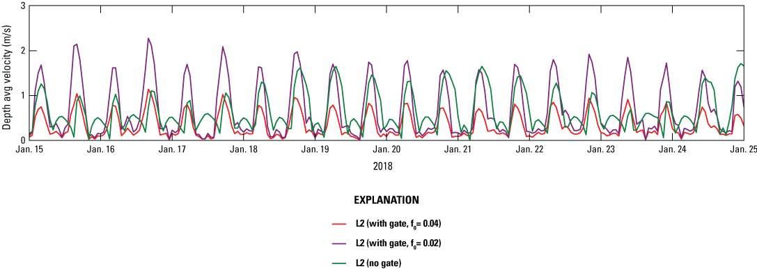
Time series of depth-averaged current speed in the Shinnecock Canal from January 15 to January 25, 2018. L2, level-2 bay-scale domain; f0, bottom friction factor; m/s, meter per second.
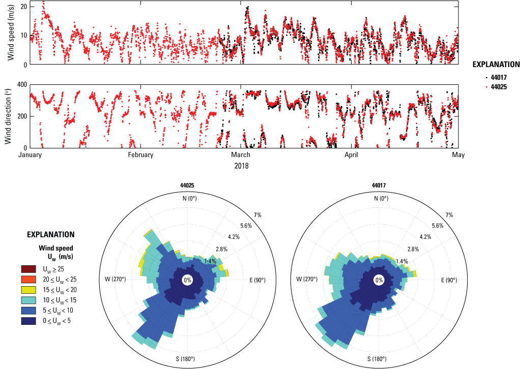
Time series of wind speed and wind direction, and wind roses from National Data Buoy Center stations 44017 and 44025 in 2018. Uw, wind speed; m/s, meter per second; ≥, greater than or equal to; ≤, less than or equal to; <, less than; °, degree; %, percent.
Treatment of Boulders
The length of the boulder line along the western facing shoreline of the Shinnecock Indian Nation is approximately 722 m. Distances between the boulders range from around 0.3 to 5 m (fig. 2). The L3 computational mesh is still too coarse to resolve the boulders, especially to the north and south of the Shinnecock Indian Nation shoreline. In the L3-FLOW model, boulders are represented as porous plates, which are groups of points in the computational grid where resistance to flow is added to the governing equations to simulate the effects of a porous structure. A quadratic friction term as below is included in the momentum equations to parameterize the force on the flow generated by the boulders:
where closs is the energy loss coefficient. Porous plates can only be defined at multiples of 45 degree angles with the grid directions. We assume that each cell with boulders features two porous plates, one in the u direction and one in the v direction. Each porous plate cell is assigned a constant closs value that partially allows for the transfer of mass and momentum across the porous plate. To the best of authors’ knowledge, the value of closs for boulders is currently unavailable. Additionally, the current reduction behind the boulders is not available, presenting challenges in the calibration of closs. In response, we ran L3-FLOW with closs = 1.0, 10.0, 40.0, and 100.0. The sensitivity of model results to different closs values is demonstrated in the results section.L3-SWAN is carried out both with and without the presence of boulders to evaluate the impact of boulders on wave height. Boulders are represented as thin walls, dams, and vegetation. Thin walls and dams are obstacles that can reduce wave height, reflect waves, and cause diffractions around their ends. A transmission coefficient (Kt), computed as below (Goda and others, 1967), is applied in the propagation terms of the action balance equation:
whereF
is the freeboard of the boulders,
Hs,i
is the incident Hs at the upwave side of the boulders, and
α and β
are two coefficients dependent on the shape of obstacles.
ρ
is the water density,
CD
is the drag coefficient,
bv
is the stem diameter,
Nv
is the population density,
hv
is the vegetation height,
h
is the water depth, and
Hrms
is the root-mean-square wave height.
In Delft3D-FLOW models, the spatial distributions of Manning’s coefficient come from the ADCIRC model used in previous surge studies (Dietrich and others, 2011). The time steps for Delft3D-FLOW models are set as 2, 0.05, and 0.005 minutes for L1, L2, and L3 domains, respectively, to ensure model stability. In SWAN models, the wind input applied in the saturation-based parameterization follows Yan (1987), and the Joint North Sea Wave Project (JONSWAP) coefficient is set as 0.038 square meter per cubic second (m2/s3) (Hasselmann and others, 1973). The depth-induced wave breaking is simulated using a constant breaker index of 0.73. The time steps of SWAN models in L1, L2, and L3 domains are all set as 1 hour.
Model Performance Metrics
To assess the model performance, the following statistical parameters are utilized: normalized root-mean-square difference (NRMSD), coefficient of determination (R2), and scatter index (SI). The definitions of these parameters are provided below:
The root-mean-square difference (RMSD) is defined as
whereN
is the sample size,
M and O
are the model results and observations, respectively, and
i
is the index in a series of data.
The coefficient of determination R2 is defined as
where the sum of squares of residual RSS is computed as . Ō is the average of the observations. The total sum of squares TSS is computed as . R2 = 1 indicates perfect agreement between the modeled and measured variables. R2 = 0 indicates that the model results are as good as random guesses around the mean of the observations. R2 is different from the square of Pearson correlation coefficient r, which measures the linear correlation of the modeled and measured variables.The scatter index (SI) is defined as
Results
Model Validation
The L1-SWAN model is validated against measurements from the NDBC station 44017, which is approximately 39,650 m southeast of Shinnecock Inlet (see figure 4 for the buoy location). The modeled wave parameters, including Hs, Tp, and θp, agree well with measurements (figs. 8, 9). The model performance metrics are summarized in table 2. Despite the relatively coarse grid at the NDBC station 44017 location, which is nearly 9 kilometers, the measured and modeled probability histograms of Tp align well (fig. 10). The probability histograms of Tp indicate a peak around 6 seconds. The presence of longer period swell waves with Tp greater than 12 seconds or shorter period waves with Tp less than 2 seconds is much less likely. The most likely Tp falls within the range of 4–9 seconds, characteristic of typical wind-driven seas. The absence of wave measurements within Shinnecock Bay prevents model validation of local-scale wave parameters. While we are unable to directly validate the L2 and L3 wave models, the strong agreement in wave parameters at NDBC station 44017 from L1-SWAN demonstrates that accurate wave boundary conditions can be transferred from L1-SWAN to L2-SWAN. The complex nearshore wave processes, such as wave breaking and wave shoaling, are considered in both L2-SWAN and L3-SWAN models along the shoreline of Shinnecock Bay. The local-scale wave dynamics and parameters in Shinnecock Bay are simulated reasonably by the Delft3D-FLOW and SWAN modeling system. Zhu and others (2023) used similar nested domains and coupled Delft3D-FLOW and SWAN models to simulate wave dynamics in upper Delaware Bay with oyster reef-based living shorelines. Local-scale field wave measurements along the Shinnecock Indian Nation shoreline could further validate the wave model and confirm the validity of this modeling system in predicting local-scale wave dynamics along the Shinnecock shoreline.
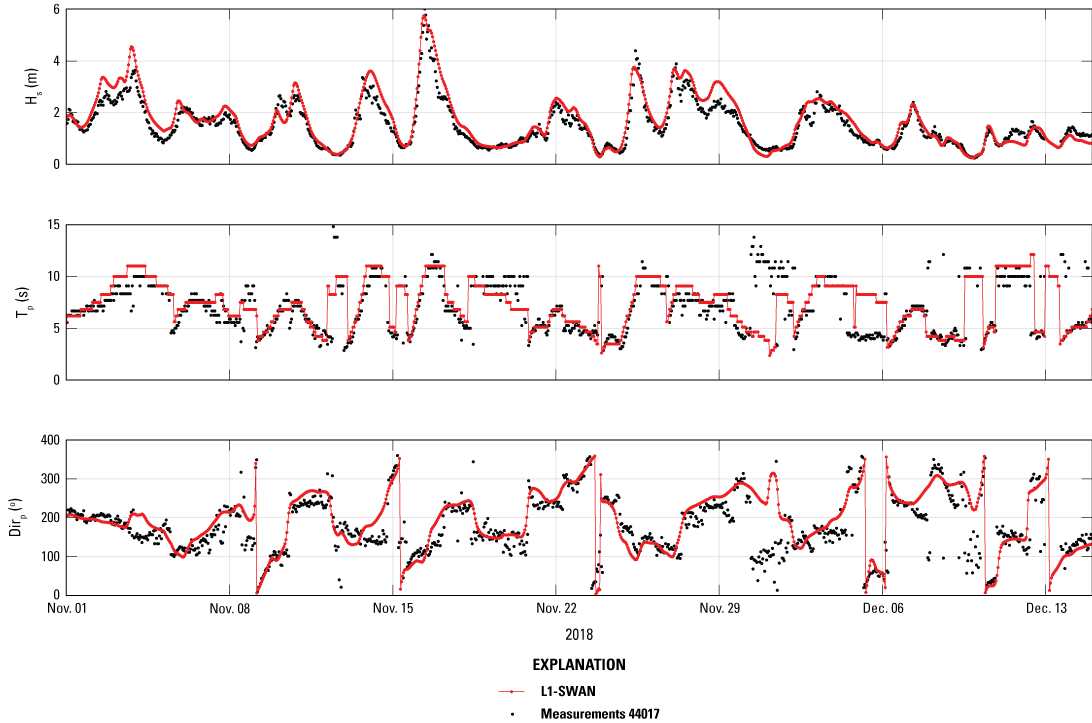
Time series of measured and modeled wave parameters at National Data Buoy Center station 44017 in 2018. HS, significant wave height; m, meter; Tp, peak wave period; s, second; Dirp, peak wave direction; °, degree; L1-SWAN, level 1 Simulating WAves Nearshore model.
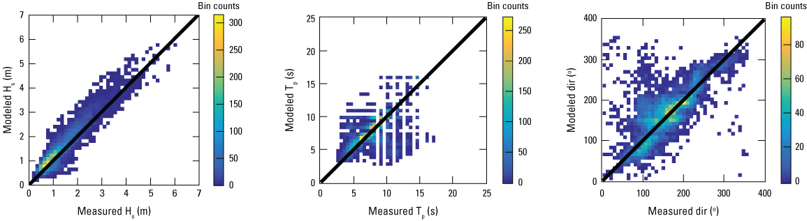
Scatter plots of measured and modeled wave parameters at National Data Buoy Center station 44017 from the level 1 Simulating WAves Nearshore model (L1-SWAN). HS, significant wave height; m, meter; Tp, peak wave period; s, second; dir, peak wave direction; °, degree.
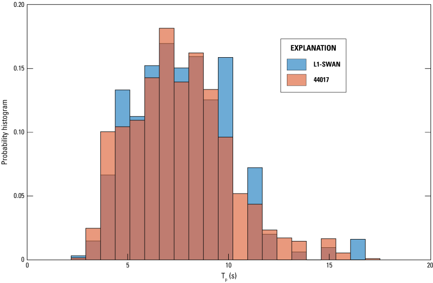
Probability histogram of measured and modeled peak wave periods at National Data Buoy Center station 44017. L1-SWAN, level 1 Simulating WAves Nearshore model; Tp, peak wave period; s, second.
Table 2.
Model statistics from the level 1 Simulating WAves Nearshore (L1-SWAN) and level 2 Delft3D-FLOW (L2-FLOW) models.[R2, coefficient of determination; NRMSD, normalized root-mean-square difference; SI, scatter index; Hs, significant wave height; %, percent; Tp, peak wave period; θp, peak wave direction; η, water level]
The modeled water level (η) from L2-FLOW is validated against measurements from the USGS station 01304746, which is close to the Ponquogue Bridge in the middle of Shinnecock Bay (see fig. 4 for station location). The modeled water level aligns well with measurements (fig. 11). The model metrics are summarized in table 2. The good agreement in water levels of L2-FLOW at USGS station 01304746 substantiates that accurate water level boundary conditions are fed into L3-FLOW from L2-FLOW, although there is no water level data near the Shinnecock Indian Nation shoreline for the L3-FLOW model calibration and validation. It should be noted that field measurements of current velocity along the shoreline in Shinnecock Indian Nation are not available; therefore, comparisons between simulated and observed current velocities for further model validation is impossible.
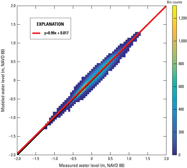
Scatter plot of measured and modeled (level 2 Delft3D-FLOW [L2-FLOW]) water levels at U.S. Geological Survey station 01304746 (USGS, 2024b). A bin count refers to the number of values that fall within each specified bin range. The red line represents the linear regression indicating the correlation between the modeled and observed data. NAVD 88, North American Vertical Datum of 1988; m, meter.
Wave Climate From L2-SWAN
Figure 12 shows the elevation map of the eastern part of Shinnecock Bay, where the offshore elevation maintains a nearly constant level of around −3.5 m (North American Vertical Datum of 1988). We selected four numerical output stations (A–D in fig. 12) along the −3.3 m (North American Vertical Datum of 1988) elevation contour and plotted the corresponding wave roses. Figure 12 depicts that the majority of offshore waves approach the Shinnecock Indian Nation shorelines at normal wave angles. The yearly average wave height in 2018 is around 0.19 m, with a standard deviation of around 0.14 m. The maximum modeled wave height in 2018 reaches 0.65 m. The wave power (P) is computed as below:
where Px and Py are the energy transport components computed internally in SWAN based on the variance density spectra. The yearly averaged P at output stations A–D are 49, 50, 48, and 44 watts per meter (W/m), respectively.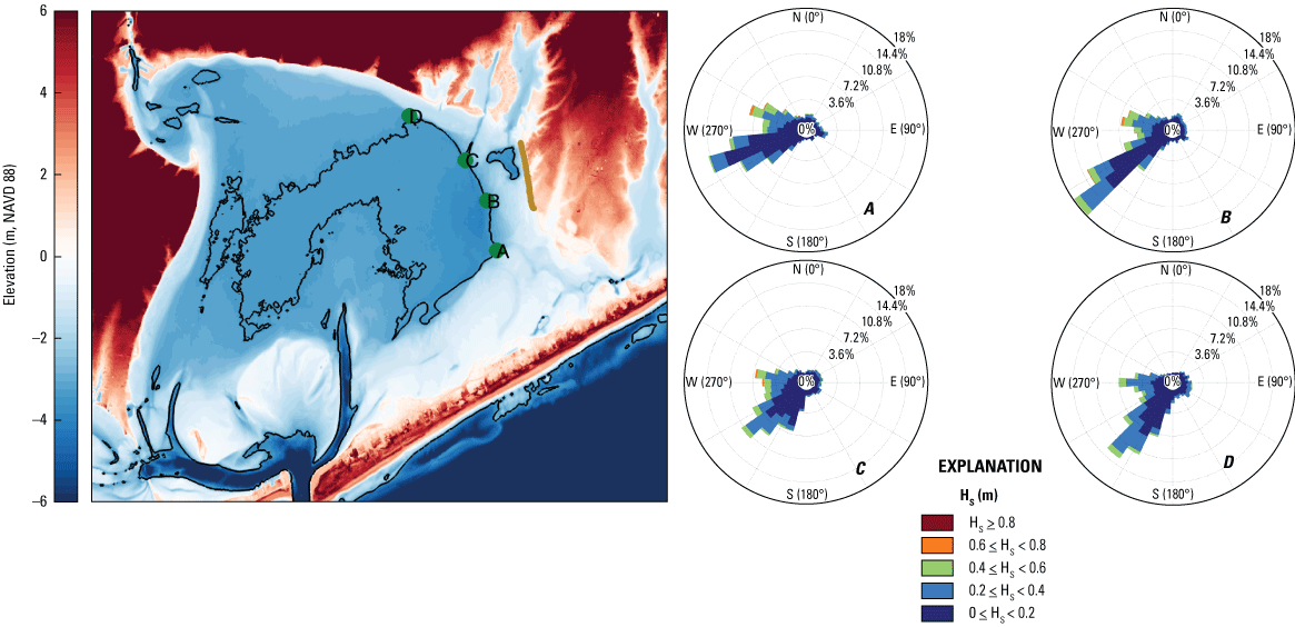
Left: Elevation map and elevation contour (black line) at −3.3 meters (North American Vertical Datum of 1988 [NAVD 88]). Four numerical output stations (A–D, marked with green dots) are selected along the contour. Right: Wave roses at these four output stations (nautical convention for the wave direction). HS, significant wave height; m, meter; ≥, greater than or equal to; ≤, less than or equal to; <, less than; °, degree; %, percent.
Boulder Effects on Currents
To illustrate the effects of boulders on currents, a baseline run without boulders is carried out in L3-FLOW. Numerical output stations are placed around the boulders as shown in figure 2. Figure 13 shows the magnitude of the daily averaged depth-averaged current (|U|) at upwave and downwave output stations corresponding to different closs. In general, the downwave |U| decreases as closs increases. Following a linear regression between the upwave and downwave daily averaged currents (U), we compute the reduction rate of the daily averaged currents as 1 − m, where m is the slope of linear regression. The sensitivity of the reduction rate to closs is illustrated in figure 14. At the output stations near the tidal ponds, a significant reduction in U is observed in the baseline run, and further reduction in U is induced by the presence of boulders. In Delft3D-FLOW, the vertical position of the porous plate is specified in terms of the model layers that it occupies. In this study, only one vertical layer is used; therefore, the boulders will always result in momentum loss regardless of the submergence. Additionally, the calibration of closs relies on the measured data in water level and depth-averaged velocity around the boulders. Due to the lack of field measurements, this study only provides a modeling analysis of the effects of boulders on currents. Simulation results show that the current velocity at the output stations could reach as high as 0.18 meter per second (m/s) without boulders as shoreline protection structures but can be reduced to less than 0.02 m/s (fig. 13). The current velocity reduction rates when closs = 100 at the case with boulders compared to the case without boulders increase from less than 20 to larger than 70 percent at the P3 and P4 stations, from less than 30 to larger than 80 percent at the P5 and P6 stations, from less than 60 to larger than 80 percent at the P7 and P8 stations, and from less than 30 to larger than 85 percent at the P9 and P10 stations, respectively (fig. 14).
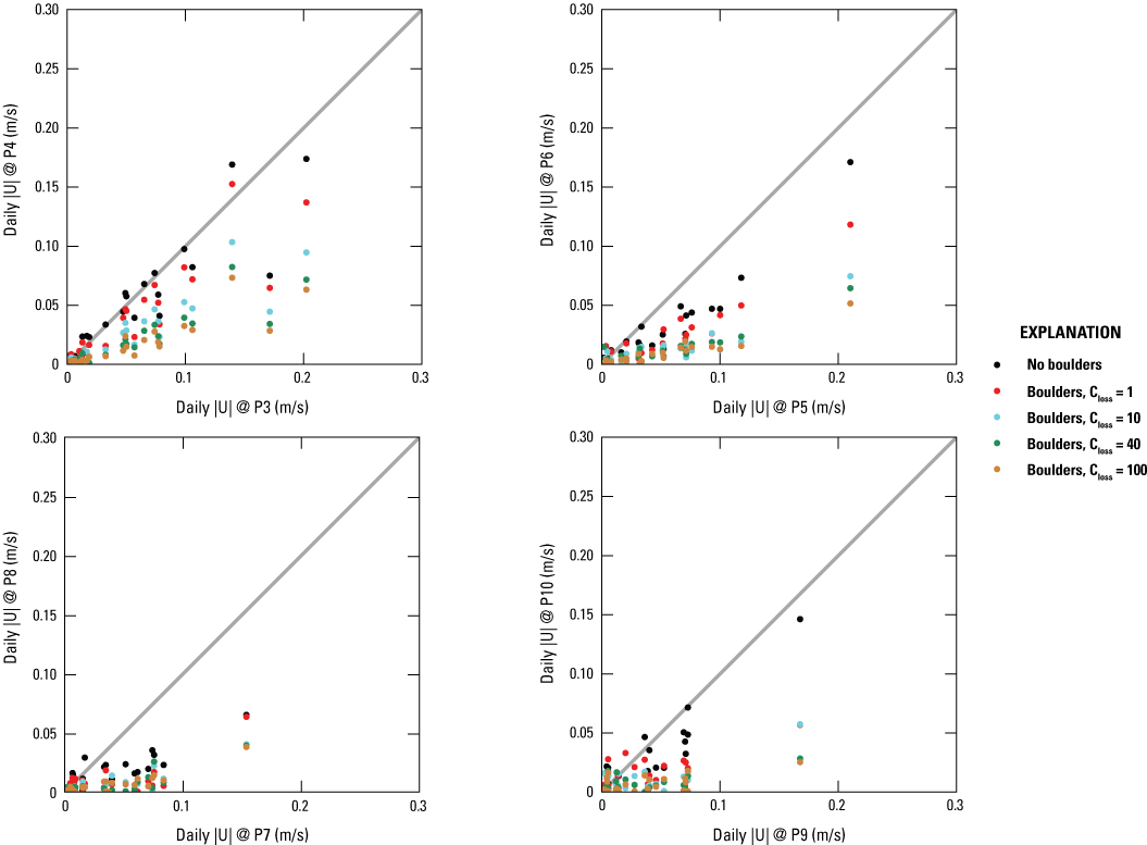
Magnitudes of the modeled daily averaged current velocity at upwave and downwave output stations. The locations of the output stations are shown in figure 2. |U|, absolute value of current velocity; @, at; P3–P10, output stations; m/s, meter per second; closs, energy loss coefficient.
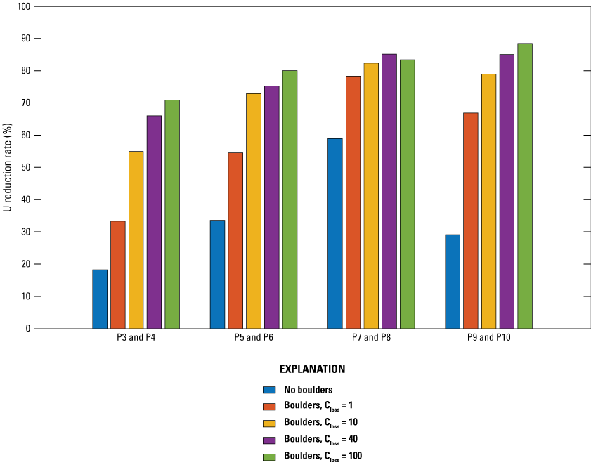
Reduction rate of daily averaged current velocity between upwave and downwave output stations. The locations of the output stations are shown in figure 2. U, value of current velocity; %, percent; P3–P10, output stations; closs, energy loss coefficient.
Boulder Effects on Waves
Model results indicate variability in longshore wave heights. Hs is generally higher near the north end of the boulders (P3 and P4 stations; refer to fig. 2 for output station locations) and lower near the tidal ponds south of the cemetery (P7 and P8 stations). Figure 15 illustrates wave height changes at the upwave and downwave sides of the boulders. Generally, wave heights decrease at the downwave side of the boulders. Wave height at the output stations in the upwave side of the boulders range between 0.35 and 0.5 m, whereas at the downwave side it can be reduced to less than 0.1 m (fig. 15). Both the dam and thin wall treatments of boulders in SWAN show similar Hs variations. The average reduction rates of Hs are 52, 15, 63, and 15 percent at P4, P6, P8, and P10 stations, respectively (fig. 15). The vegetation treatment of boulders results in generally smaller Hs reduction. The reduction rates are 16, 13, 63, and 26 percent at P4, P6, P8, and P10 stations, respectively (fig. 15). In addition to wave-height reduction, wave amplification is also observed in the model results. To illustrate the effects of boulders on wave transformation, a baseline run without boulders is carried out in L3-SWAN. The model results considering boulders are then compared with baseline model results (see fig. 16). At the north end, the dam and thin wall treatments of boulders result in a 44 percent reduction in Hs, while the vegetation treatment (treating boulders as vegetation) of boulders only leads to a 2 percent reduction in Hs. At the south end, the dam, thin wall, and vegetation treatments of boulders lead to 5, 2, and 2 percent reductions in Hs, respectively. Near the two tidal ponds, boulders do not cause Hs changes on average.
The yearly averaged wave power at the upwave side of the boulders varies from 2 (P7 station) to 35 (P3 station) W/m, with the smallest yearly averaged wave power found near the tidal pond south of the cemetery. In the baseline run, the yearly averaged wave power is reduced to 25, 3, 0.2, and 10 W/m at P4, P6, P8, and P10 stations, respectively (fig. 17). Treating boulders as dams or thin walls leads to additional wave power reductions of 13, 0.02, 0.01, and 1 W/m at P4, P6, P8, and P10 stations, respectively (fig. 17). Treating boulders as vegetation leads to additional wave power reductions of 3, 0.2, 0.01, and 4 W/m at P4, P6, P8, and P10 stations, respectively (fig. 17). The annual wave power reduction around the boulders is consistent with the wave height variations, with boulders causing significant annual wave power reduction near the north end, nearly unchanged annual wave power near the two tidal ponds, and small annual wave power reduction near the south end of the boulders.
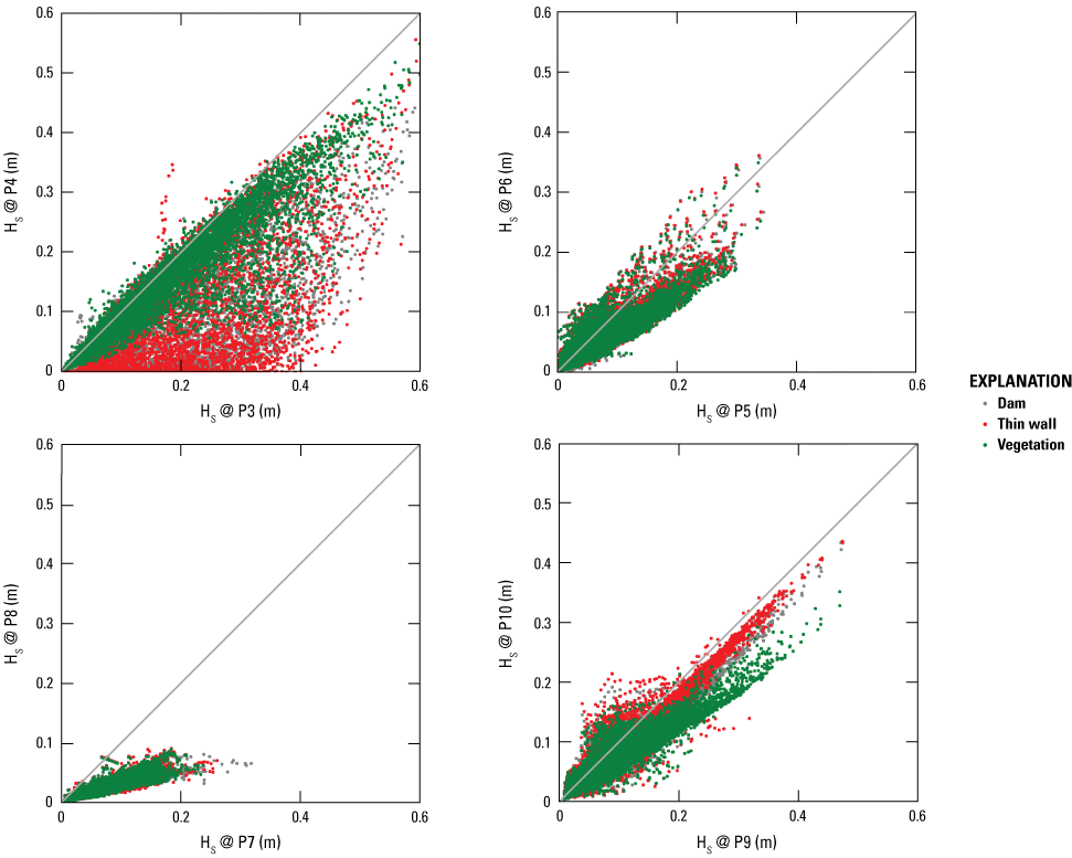
Modeled wave height at upwave and downwave output stations. HS, significant wave height; @, at; P3–P10, output stations; m, meter.
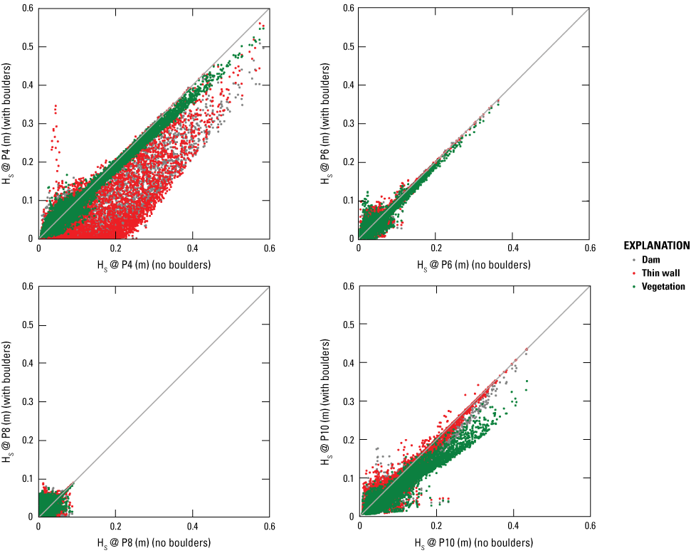
Modeled wave height with and without boulders in the level 3 Simulating WAves Nearshore model (L3-SWAN) at downwave output stations. HS, significant wave height; @, at; P4, P6, P8, and P10, output stations; m, meter.
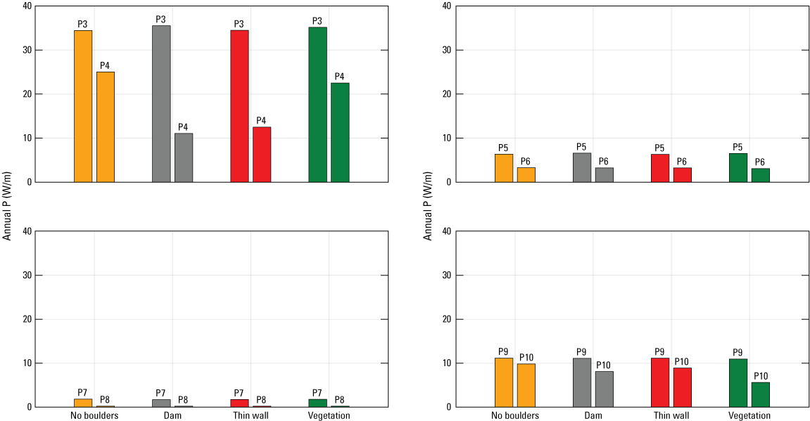
Modeled annual wave power at upwave and downwave output stations. P, wave power; P3–P10, output stations; W/m, watt per meter.
Discussions
Effect of Living Shoreline Structures on Wave Dynamics
Simulation results show that wave height decreases at the downwave side of the boulders along the Shinnecock Indian Nation shoreline, indicating that the boulders are generally effective in attenuating wave energy. There are large local variabilities in wave height and wave power reduction from upwave output stations to downwave output stations. Reductions in wave height tend to be larger at the northern end of the boulders where larger wave heights are found when compared to the southern end of the boulders. The variations in wave height reduction result from a combined effect of bathymetric changes around boulders. This is consistent with findings from literature on oyster reef-based living shoreline structures that wave attenuation by living shoreline structures is dependent on water depth, wind speed, wind direction, and local bathymetry (Wiberg and others, 2019; Zhu and others, 2020; Wang and others, 2021, 2023).
Model results also indicate wave amplification—this is consistent with the field measurements associated with oyster reef-based living shoreline structures in Gandys Beach (Zhu and others, 2020). Zhu and others (2020) revealed that constructed oyster reefs do not necessarily induce wave-height reduction, and wave amplification occurs due to wave shoaling, wave diffraction, and wave focusing. It is found that treating boulders as dam, thin wall, or vegetation leads to different magnitudes in reductions of wave height and wave power, demonstrating that different shoreline structures have various effects in wave attenuation. The vegetation treatment of boulders results in smaller wave-height reduction because it does not induce wave breaking when the boulder freeboard approaches zero.
Effect of Living Shoreline Structures on Current Dynamics
Simulation results show that current velocities from bayside of the boulders to leeside of the boulders along the Shinnecock Indian Nation shoreline are reduced more with the boulders compared with the case without the placement of boulders. Moreover, reductions in current velocities along the Shinnecock Indian Nation shoreline tend to vary with locations on the shoreline. Compared with the no-boulder case, current velocity reductions with the boulders are found to be larger at the output stations that are located on the sections far away from the large boulder gaps (for example, P3 and P4 stations and P9 and P10 stations) than those at the stations at or close to the boulder gaps (for example, P5 and P6 stations and P7 and P8 stations) (fig. 2). These results indicate that the boulders are effective in changing tidal circulation and reducing current velocity, and that there are local variabilities in a boulder’s capacity in current velocity reduction. This finding is consistent with previous living shoreline velocity studies (Wang and others, 2021; Salatin and others, 2022; Wang and others, 2023). Current velocities are found to decline at leeside of the constructed oyster reefs along the Gandys Beach (Wang and others, 2021; Salatin and others, 2022) and Chincoteague (Wang and others, 2023) shorelines, and such velocity reductions by the oyster reefs vary in space and time. Current velocity reductions along the living shorelines are complex and dependent on wind and wave conditions, tidal phase (ebb versus flood), location of measurements relative to the structures, and geomorphological features (Wang and others, 2023).
In this study, although there are no field data to determine which closs is representative of the field condition, current velocities in the leeside of the boulders along the Shinnecock Indian Nation shorelines are found to be reduced compared with the bayside of the boulders at the output stations. This result is different from previous studies on current velocity change along the living shorelines using oyster reef-based structure. For example, in Gandys Beach, Virginia (Salatin and others, 2022), and Little Toms Cove, Virginia (Wang and others, 2023), velocities behind the oyster castles can be increased at locations near the boundary between the castles and open water, especially during ebb tides. The discrepancies in structure-induced velocity changes between this study and previous studies can be attributed to the difference in structure configuration as well as the absence of wave-driven currents in this modeling study. The circulation pattern may be altered if the gaps between the oyster castles are larger than the gaps between the boulders (Wang and others, 2021).
Implications for Coastal Management and Restoration Projects
This study demonstrates the offshore wave climate near Shinnecock Indian Nation and quantifies the effects of the existing large boulders on wave attenuation through process-based numerical models. Along the Shinnecock Indian Nation shoreline, wave-height reduction varies along the boulder-protected shoreline, indicating that some sections of shoreline have not benefitted from the boulders. Adjusting the configuration of the existing boulders—for example, by increasing the crest height or the density—at these shoreline sections could help to reduce erosion. Another method for structure adjustment is the utilization of oyster reef-based materials such as constructed oyster castles, oyster shell bags, and cages. This is based on the improvement of current velocity by the construction of the boulders along the Shinnecock Indian Nation shoreline, which is one critical habitat suitability metric for optimizing oyster larval transport, recruitment, and oyster growth. A current velocity threshold of 0.15 m/s is used for optimal oyster growth in oyster reef-based living shoreline assessment (for example, Salatin and others, 2022) and lower thresholds of 0.07 and 0.1 m/s are also determined from oyster growth experiments (for example, literature review in Wang and others [2017b]). In this study, simulated current velocities are found to decrease from larger than 0.15 m/s in the bayside of the boulders (upwave output stations) to less than 0.1 m/s in the leeside of the boulders (downwave output stations).
Other habitat suitability metrics, such as salinity and temperature, could also be considered when applying oyster reef-based structures (with boulders) for enhancing the effectiveness of the living shoreline structures. Seagrasses planted around/near the boulders can also be used to make boulders more effective as living shoreline structures. A numerical modeling study for living shorelines in the Chesapeake Bay using Delft3D-FLOW and SWAN models found that erosion can be drastically reduced when combining riprap, salt marsh, and submerged aquatic vegetation as the living shoreline structures (Vona and others, 2021). The Shinnecock Indian Nation also considered other living components including the construction of oyster reefs built from shell or concrete and the planting of seagrass (for example, eelgrass) to enhance shoreline protection and restoration (for example, Anchor QEA, LLC, The Nature Conservancy, and Fine Arts and Sciences, LLC, 2019). Directly south of the Cuffee Beach parking area, old oyster cages have been placed to attenuate wave energy from large coastal storms, reduce erosion, and facilitate sand accretion. Oysters have been farmed on the eastern side of Shinnecock Bay by the Shinnecock Indian Nation for many years and were introduced in the western part of the bay as part of a research and restoration program in 2017 (Ahn and Ronan, 2020). Regardless of the types of living shoreline structures that may be used along the Shinnecock Indian Nation shoreline, the model framework developed in this study can be leveraged for optimal design of nature-based solutions, which can guide where to install living shoreline structures and how to determine their optimal size.
Data and Knowledge Gaps
The reduction in wave height and wave power along the Shinnecock Indian Nation shoreline on a local scale is determined by the L3-SWAN model. Due to the lack of measured wave and velocity data around the boulders, L3-SWAN model simulations could not be validated. This study provides a modeling analysis of the potential effects of boulders or similar structures on currents and waves. The lack of hydrodynamic and wave data hinders the calibration and validation of wave and flow models, limiting our ability to assess and predict local-scale wave dynamics accurately. Addressing this data gap could help to enhance the reliability and effectiveness of hydrodynamic and wave models and could provide valuable insight into the local wave-climate and estuarine circulation—these validated models can help to facilitate informed decision making by the Shinnecock Indian Nation and various stakeholders in the region.
This numerical study reveals that wave and flow measurements near the Shinnecock Indian Nation shoreline, particularly at the coastal restoration project site (for example, boulders and beaches), can help to enhance the understanding of wave climate and coastal processes and calibrate and validate wave models (for example, SWAN in this study). In addition to analyzing wave-height variations from offshore to nearshore, and around the structures, wave-spectral analysis could be conducted to investigate wave-spectral variations. A similar analysis was completed for the oyster reef-based living shoreline near Gandys Beach (upper Delaware Bay) by Zhu and others (2020), which indicated that the energy transfer from the primary waves to the high harmonics after waves propagates over the submerged oyster reefs and revealed that swell energy originated from the Atlantic Ocean can penetrate oyster reefs without any dampening. Current measurements are lacking to calibrate and validate circulation models (for example, Delft3D-FLOW in this study). Boulder dimensions, including the cross-sectional areas, heights, gap width, and population density, are lacking for boulder implementations in numerical models. The nearshore bathymetry and topography are outdated, and thus, surveys and updates in numerical models could help to achieve higher model accuracy. The field data can also be employed in data-driven models, such as the bagged regression tree algorithm (Wang and others, 2022; Zhu and others, 2023) to improve the accuracy of physics-based models at locations where field measurements are available.
Further Research Opportunities
This study found local variabilities in current velocity and wave height and wave energy along the Shinnecock Indian Nation shoreline, and therefore, field measurements of current velocity and wave parameters at multiple locations in both the bayside and leeside of the boulders over the storm periods could help improve the accuracy of the hydrodynamic and wave modeling. Since the main goal of living shorelines is to protect shoreline from wave and current induced sediment erosion and shoreline retreat, the in situ measurements of sediment movement including sediment transport, erosion, deposition, and trapping by vegetation from offshore to onshore with and without living shoreline structures (large boulders for Shinnecock Indian Nation shoreline in this study) could help improve the understanding of sediment dynamics. With field sediment measurements, sediment budget can be determined to inform effective management of sediment along the Shinnecock Indian Nation shoreline and beaches. By integrating sediment dynamics with current and wave dynamics along the Shinnecock Indian Nation shoreline, direct relationships between wave energy and shoreline retreat rates can be explored (Marani and others, 2011; Wang and others, 2023; Zhu and others, 2023). With field sediment data, models of geomorphology for shorelines, beaches, and salt marshes in Shinnecock Indian Nation can be developed to assess and predict the morphological changes in Shinnecock Indian Nation tidal wetlands including shorelines under future storms and sea level rise (Wang and others, 2017a). The modeling system developed in this study can serve as a tool for simulating and analyzing the impacts of major tropical storms and hurricanes. Future studies may utilize this system to better understand the dynamics of extreme weather events and the effectiveness of boulders for shoreline protection and enhance preparedness and response strategies.
Improvement of water quality and habitat for fish and wildlife species and other ecological services are the ecological goals of living shorelines. Oyster reef-based structures and seagrass are considered in Shinnecock Indian Nation living shoreline protection and restoration (Shinnecock Indian Nation, 2013). Field measurements of water quality parameters such as salinity, temperature, dissolved oxygen, total suspended solids, and chlorophyll-a concentrations can help to determine if the habitat suitability for oysters and seagrass species in the estuaries could be improved by implementation of the living shoreline structures (Wang and others, 2023). Field water quality measurements and process-driven water quality models for the Shinnecock Indian Nation estuary can be coupled with the hydrodynamic and wave models (Delft3D-FLOW and SWAN in this study) and validated and used to predict habitat changes in the Shinnecock Indian Nation estuary with and without living shoreline structures under future storms and sea level rise conditions.
Summary
A numerical study based on physics-based hydrodynamic models was conducted to simulate circulation and wave dynamics along the shoreline of Shinnecock Indian Nation. The hydrodynamic model Delft3D-FLOW and the spectral-wave model Simulating WAves Nearshore (SWAN) are coupled in three-level nested domains. The mesh resolution along the Shinnecock shoreline is refined from 6,300 meters (m) (the first level domain) to 0.9 m (the third level domain). This numerical study sheds light on the wave climate along the shoreline of Shinnecock Indian Nation and elucidates the effectiveness of existing boulders along the shoreline for wave attenuation. The findings contribute not only to the scientific understanding of wave environment but also offer practical insights for resilient coastal management. This research can inform strategies for safeguarding vulnerable coastal communities and promoting climate change adaption, resilience, and sustainability of the habitat and ecosystem along the Shinnecock shoreline. The key findings of this study are summarized as below:
The numerical model framework developed in this study can simulate the circulation and wave environment in Shinnecock Bay and the Shinnecock shoreline; however, field measurements, such as wave and current observations, are lacking for model calibration and validation, in particular for the parametrization of boulder effects.
-
• Different treatments of boulders in SWAN (that is, dams, thin walls, and vegetation) result in different wave attenuation. Overall, the dam and thin wall treatments of boulders result in a higher reduction rate in significant wave height (Hs) than the vegetation treatment of boulders.
-
• Numerical model results show that the offshore yearly averaged wave power along the −3.3 m (North American Vertical Datum of 1988) elevation contour near the Shinnecock shoreline ranges from 44 to 50 watts per meter. The yearly averaged wave power in nearshore is reduced due to the combined effects of bathymetric changes and the placement of boulders. The contribution of boulders to annual wave power reduction is smaller near the tidal pond south of the cemetery and greater at the north end of the boulders.
-
• This study provides a modeling analysis of the potential effects of boulders or similar structures on currents and waves. Field measurements regarding waves, currents, and water levels at the upwave and downwave sides of the boulders, together with the boulder dimensions, could help to calibrate the numerical models for accuracy improvement.
References Cited
Ahn, J.E., and Ronan, A.D., 2019, Impact of discrepancies between global ocean tide models on tidal simulations in the Shinnecock Bay area: Journal of Waterway, Port, Coastal, and Ocean Engineering, v. 145, no. 2, article 04018042, 14 p., accessed October 8, 2023, at https://doi.org/10.1061/(ASCE)WW.1943-5460.0000500.
Ahn, J.E., and Ronan, A.D., 2020, Development of a model to assess coastal ecosystem health using oysters as the indicator species: Estuarine, Coastal and Shelf Science, v. 233, article 106528, accessed October 27, 2023, at https://doi.org/10.1016/j.ecss.2019.106528.
Anchor QEA, LLC, The Nature Conservancy, and Fine Arts and Sciences, LLC, 2019, Shinnecock Indian Nation climate vulnerability assessment and action plan: Peconic Estuary Program and Shinnecock Indian Nation, prepared by Anchor QEA, LLC, The Nature Conservancy, and Fine Arts and Sciences, LLC, 35 p., accessed September 15, 2023, at https://www.peconicestuary.org/wp-content/uploads/2019/10/Shinnecock-Indian-Nation-Climate-Vulnerability-Assessment-and-Action-Plan.pdf.
Buonaiuto, F., and Militello, A., 2003, Coupled circulation, wave, and morphology-change modeling—Shinnecock Inlet, New York, in Estuarine and Coastal Modeling, International Conference, 8th, Monterey, California, November 3–5, 2003, [Proceedings]: Reston, Virginia, American Society of Civil Engineers, p. 819–838.
Capurso, W.D., Noll, M.L., and Chu, A., 2024, Three-dimensional point cloud data collected with a scanning total station on the western shoreline of the Shinnecock Nation Tribal lands, Suffolk County, New York, 2022: U.S. Geological Survey data release, https://doi.org/10.5066/P9OG0AAO.
Dietrich, J.C., Westerink, J.J., Kennedy, A.B., Smith, J.M., Jensen, R.E., Zijlema, M., Holthuijsen, L.H., Dawson, C., Luettich, R.A., Powell, M.D., Cardone, V.J., Cox, A.T., Stone, G.W., Pourtaheri, H., Hope, M.E., Tanaka, S., Westerink, L.G., Westerink, H.J., and Cobell, Z., 2011, Hurricane Gustav (2008) waves and storm surge—Hindcast, synoptic analysis, and validation in southern Louisiana: Monthly Weather Review, v. 139, no. 8, p. 2488–2522.
Hague, B., McGregor, S., Murphy, B.F., Reef, R., and Jones, D.A., 2020, Sea level rise driving increasingly predictable coastal inundation in Sydney, Australia: Earth’s Future, v. 8, no. 9, article e2020EF001607, 17 p., accessed October 28, 2023, at https://doi.org/10.1029/2020EF001607.
Hasselmann, K., Barnett, T., Bouws, E., Carlson, H., Cartwright, D., Enke, K., Ewing, H., Gienapp, J.A., Hasselmann, D., Kruseman, P., Meerburg, A., Müller, P., Olbers, D., Richter, K., Sell, W., and Walden, H., 1973, Measurements of wind-wave growth and swell decay during the Joint North Sea Wave Project (JONSWAP): Hamburg, Germany, Deutches Hydrographisches Institut, 94 p.
Huff, T.P., Feagin, R.A., and Figlus, J., 2022, Delft3D as a tool for living shoreline design selection by coastal managers: Frontiers in Built Environment, v. 8, article 926662, 12 p., accessed September 6, 2023, at https://doi.org/10.3389/fbuil.2022.926662.
Lin, L., Demirbilek, Z., Greenblatt, E., Rice, S., and Buonaiuto, F., 2022, Numerical modeling of Shinnecock Inlet, New York, for coastal erosion control support and inlet sediment management, in Conference on Coastal Engineering, 37th, Sydney, Australia, December 4–9, 2022, [Proceedings]: International Conference on Coastal Engineering [ICCE], v. 37, paper 51, 13 p.
Luettich, R., Westerink, J., and Scheffner, N., 1992, ADCIRC—An advanced three-dimensional circulation model for shelves, coasts, and estuaries—Report 1. Theory and methodology of ADCIRC-2DDI and ADCIRC-3DL: Vicksburg, Mississippi, U.S. Army Corps of Engineers, Waterways Experiment Station, Dredging Research Program Technical Report DRP–92–6, 137 p.
Marani, M., D’Alpaos, A., Lanzoni, S., and Santalucia, M., 2011, Understanding and predicting wave erosion of marsh edges: Geophysical Research Letters, v. 38, no. 21, article L21401, 5 p., accessed January 15, 2024, at https://doi.org/10.1029/2011GL048995.
Militello, A., and Kraus, N.C., 2001, Shinnecock Inlet, New York, site investigation report 4—Evaluation of flood and ebb shoal sediment source alternatives for the west of Shinnecock Interim Project, New York: Vicksburg, Mississippi, Engineer Research and Development Center, Coastal and Hydraulics Lab, Report ERDC/CHL–TR–98–32, 212 p.
Morris, R.L., La Peyre, M.K., Webb, B.M., Marshall, D.A., Bilkovic, D.M., Cebrian, J., McClenachan, G., Kibler, K.M., Walters, L.J., Bushek, D., Sparks, E.L., Temple, N.A., Moody, J., Angstadt, K., Goff, J., Boswell, M., Sacks, P., and Swearer, S.E., 2021, Large-scale variation in wave attenuation of oyster reef living shorelines and the influence of inundation duration: Ecological Applications, v. 31, no. 6, article e02382, 15 p., accessed January 9, 2024, at https://doi.org/10.1002/eap.2382.
National Oceanic and Atmospheric Administration [NOAA] National Geophysical Data Center, 1999, U.S. coastal relief model 1—Northeast Atlantic: NOAA National Centers for Environmental Information web page, accessed December 20, 2023, at http://dx.doi.org/10.7289/V5MS3QNZ.
O’Donnell, J.E.D., 2017, Living shorelines—A review of literature relevant to New England coasts: Journal of Coastal Research, v. 33, no. 2, p. 435–451, accessed December 6, 2023, at https://doi.org/10.2112/JCOASTRES-D-15-00184.1.
Salatin, R., Wang, H., Chen, Q., and Zhu, L., 2022, Assessing wave attenuation with rising sea levels for sustainable oyster reef-based living shorelines: Frontiers in Built Environment, v. 8, article 884849, accessed January 10, 2024, at https://doi.org/10.3389/fbuil.2022.884849.
Sanchez, A., Wu, W., Li, H., Brown, M., Reed, C., Rosati, J., and Demirbilek, Z., 2014, Coastal Modeling System—Mathematical formulations and numerical methods: U.S. Army Corps of Engineers, Engineer Research and Development Center, Coastal and Hydraulics Laboratory, Technical Report ERDC/CHL TR–14–2, 104 p.
Seelig, W., 1979, Effects of breakwaters on waves—Laboratory tests of wave transmission by overtopping, p. 941–961 in Coastal Structures 79, A Specialty Conference on the Design Construction, Maintenance and Performance of Port and Coastal Structures, Alexandria, Virginia, March 14–16, 1979, [Proceedings]: American Society of Civil Engineers [ASCE], Waterway, Port, Coastal and Ocean Division, v. 2, 1,211 p.
Shinnecock Indian Nation, 2013, Shinnecock Indian Nation climate change adaptation plan, October 2013: Shinnecock Indian Nation, 25 p., accessed September 15, 2023, at https://www.cakex.org/sites/default/files/documents/shinnecock_nation_ccadaptation_plan_9.27.13.pdf.
Sutton-Grier, A.E., Wowk, K., and Bamford, H., 2015, Future of our coasts—The potential for natural and hybrid infrastructure to enhance the resilience of our coastal communities, economies and ecosystems: Environmental Science & Policy, v. 51, p. 137–148, accessed December 5, 2023, at https://doi.org/10.1016/j.envsci.2015.04.006.
U.S. Geological Survey [USGS], 2024a, USGS 01304562 Peconic River at County Hwy 105 at Riverhead NY, in USGS water data for the Nation: U.S. Geological Survey National Water Information System database, accessed January 9, 2024, at https://doi.org/10.5066/F7P55KJN. [Site information directly accessible at https://waterdata.usgs.gov/nwis/inventory/?site_no=01304562.]
U.S. Geological Survey [USGS], 2024b, USGS 01304746 Shinnecock Bay at Ponquogue NY, in USGS water data for the Nation: U.S. Geological Survey National Water Information System database, accessed January 9, 2024, at https://doi.org/10.5066/F7P55KJN. [Site information directly accessible at https://waterdata.usgs.gov/nwis/inventory/?site_no=01304746.]
Vona, I., Palinkas, C., and Nardin, W., 2021, Sediment exchange between the created saltmarshes of living shorelines and adjacent submersed aquatic vegetation in the Chesapeake Bay: Frontiers in Marine Science, v. 8, article 727080, 17 p., accessed October 18, 2023, at https://doi.org/10.3389/fmars.2021.727080.
Wang, H., Capurso, W., Chen, Q., Zhu, L., Niemoczynski, L., and Snedden, G., 2021, Assessment of wave attenuation, current patterns, and sediment deposition and erosion during winter storms by living shoreline structures in Gandys Beach, New Jersey: U.S. Geological Survey Open-File Report 2021–1040, 37 p., accessed May 8, 2023, at https://doi.org/10.3133/ofr20211040.
Wang, H., Chen, Q., Capurso, W.D., Niemoczynski, L.M., Wang, N., Zhu, L., Snedden, G.A., Whitbeck, M., Wilson, C.A., and Brownley, M., 2024, Monitoring of wave, current, and sediment dynamics along the Fog Point living shoreline, Glenn Martin National Wildlife Refuge, Maryland: U.S. Geological Survey Open-File Report 2024–1004, 32 p., accessed February 16, 2024, at https://doi.org/10.3133/ofr20241004.
Wang, H., Chen, Q., Hu, K., Snedden, G.A., Hartig, E.K., Couvillion, B.R., Johnson, C.L., and Orton, P.M., 2017a, Numerical modeling of the effects of Hurricane Sandy and potential future hurricanes on spatial patterns of salt marsh morphology in Jamaica Bay, New York City: U.S. Geological Survey Open-File Report 2017–1016, 43 p., accessed October 18, 2023, at https://doi.org/10.3133/ofr20171016.
Wang, H., Chen, Q., La Peyre, M.K., Hu, K., and La Peyre, J.F., 2017b, Predicting the impacts of Mississippi River diversions and sea-level rise on spatial patterns of eastern oyster growth rate and production: Ecological Modelling, v. 352, p. 40–53, accessed November 20, 2023, at https://doi.org/10.1016/j.ecolmodel.2017.02.028.
Wang, H., Chen, Q., Wang, N., Capurso, W.D., Niemoczynski, L.M., Zhu, L., Snedden, G.A., Holcomb, K.S., Lusk, B.W., Wilson, C.A., and Cornell, S.R., 2023, Monitoring of wave, current, and sediment dynamics along the Chincoteague living shoreline, Virginia: U.S. Geological Survey Open-File Report 2023–1020, 32 p., accessed April 6, 2023, at https://doi.org/10.3133/ofr20231020.
Wang, N., Chen, Q., Zhu, L., and Wang, H., 2022, Data-driven modeling of wind waves in upper Delaware Bay with living shorelines: Ocean Engineering, v. 257, article 111669, 17 p., accessed September 1, 2023, at https://doi.org/10.1016/j.oceaneng.2022.111669.
Wiberg, P.L., Taube, S.R., Ferguson, A.E., Kremer, M.R., and Reidenbach, M.A., 2019, Wave attenuation by oyster reefs in shallow coastal bays: Estuaries and Coasts, v. 42, no. 2, p. 331–347, accessed December 10, 2023, at https://doi.org/10.1007/s12237-018-0463-y.
Zhu, L., Chen, Q., Wang, H., Wang, N., Hu, K., Capurso, W., Niemoczynski, L., and Snedden, G., 2023, Modeling surface wave dynamics in upper Delaware Bay with living shorelines: Ocean Engineering, v. 284, article 115207, 17 p., accessed October 18, 2023, at https://doi.org/10.1016/j.oceaneng.2023.115207.
Datums
Vertical coordinate information is referenced to the North American Vertical Datum of 1988 (NAVD 88).
Horizontal coordinate information is referenced to the North American Datum of 1983 (NAD 83).
Elevation, as used in this report, refers to distance above the vertical datum.
For more information about this publication, contact
Director, Wetland and Aquatic Research Center
U.S. Geological Survey
700 Cajundome Blvd.
Lafayette, LA 70506–3152
For additional information, visit
https://www.usgs.gov/centers/wetland-and-aquatic-research-center-warc
Publishing support provided by
Lafayette Publishing Service Center
Disclaimers
Any use of trade, firm, or product names is for descriptive purposes only and does not imply endorsement by the U.S. Government.
Although this information product, for the most part, is in the public domain, it also may contain copyrighted materials as noted in the text. Permission to reproduce copyrighted items must be secured from the copyright owner.
Suggested Citation
Zhu, L., Wang, H., Chen, Q., Capurso, W., and Noll, M., 2024, Numerical modeling of circulation and wave dynamics along the shoreline of Shinnecock Indian Nation in Long Island, New York: U.S. Geological Survey Open-File Report 2024–1050, 32 p., https://doi.org/10.3133/ofr20241050.
ISSN: 2331-1258 (online)
Study Area
| Publication type | Report |
|---|---|
| Publication Subtype | USGS Numbered Series |
| Title | Numerical modeling of circulation and wave dynamics along the shoreline of Shinnecock Indian Nation in Long Island, New York |
| Series title | Open-File Report |
| Series number | 2024-1050 |
| DOI | 10.3133/ofr20241050 |
| Publication Date | August 30, 2024 |
| Year Published | 2024 |
| Language | English |
| Publisher | U.S. Geological Survey |
| Publisher location | Reston, VA |
| Contributing office(s) | Wetland and Aquatic Research Center |
| Description | Report: viii, 32 p.; Data Release |
| Country | United States |
| State | New York |
| Other Geospatial | Shinnecock Indian Nation relative to Shinnecock Bay |
| Online Only (Y/N) | Y |