

Quantifying Potential Effects of China’s Gallium and Germanium Export Restrictions on the U.S. Economy
Links
- Document: Report (2.77 MB pdf) , HTML , XML
- Download citation as: RIS | Dublin Core
Acknowledgments
At the time of publication, detailed input-output tables for 2021 were not publicly available from the Bureau of Economic Analysis. The authors would like to thank Joshua Coyan, Michael George, Daniel Hayba, and Steve Textoris at the U.S. Geological Survey for reviews and feedback.
Abstract
China’s export controls on gallium and germanium exemplify concerns regarding the reliability of supplies of mineral commodities that are essential to economic development, national security, and transition to renewable energy. This report presents a new model that quantifies the potential effects of mineral commodity supply disruptions on the U.S. economy. After calculating postdisruption equilibrium prices and quantities, a nonlinear optimization routine was used along with economic input-output tables to estimate the effects of varying Chinese net export restrictions of gallium and germanium on U.S. gross domestic product (GDP). The results indicated that a complete restriction of China’s net exports of gallium and germanium could cause the U.S. GDP to decrease by $3.1 billion (with lower and upper estimates of $1.7 billion to $8.2 billion) and $0.4 billion ($0.01 billion to $1.1 billion), respectively, if disrupted separately, and $3.4 billion ($1.7 billion to $9.0 billion) if disrupted simultaneously. The proposed model can be applied to other commodities and disruption scenarios.
Plain Language Summary
China’s export controls on gallium and germanium illustrate concerns about the reliability of supplies of mineral commodities that are essential to economic development, national security, and transitioning to renewable energy. The U.S. Geological Survey created a new model to quantify the potential effects of mineral commodity supply disruptions from Chinese net export restrictions of gallium and germanium on U.S. gross domestic product (GDP). The results indicated that a complete restriction of China’s net exports of gallium and germanium could cause the U.S. GDP to decrease by $3.1 billion (with lower and upper estimates of $1.7 billion to $8.2 billion) and $0.4 billion ($0.01 billion to $1.1 billion), respectively, if disrupted separately, and $3.4 billion ($1.7 billion to $9.0 billion) if disrupted simultaneously. The proposed model can be applied to other commodities and disruption scenarios.
Introduction
Reliable supplies of mineral commodities are essential to the functioning of an interconnected global economy. Yet in the past several years, mineral commodity supply chains have faced considerable strain from the COVID–19 pandemic (Jowitt, 2020), the Russia-Ukraine conflict (Khurshid and others, 2023), as well as trade tensions among the world’s leading industrial nations (Gulley and others, 2018; Kalantzakos, 2020). These strains come at a time when demand for certain mineral commodities may grow considerably with the transition to renewable energy sources, increased urbanization, and the accelerating adoption of various technologies, including artificial intelligence, fifth-generation (5G) wireless cellular technology, and autonomous vehicles, among others (Nassar, 2023). Recent actions by the government of the People’s Republic of China to impose export controls on various gallium and germanium products (Ministry of Commerce and General Administration of Customs [China], 2023)—metals, compounds, and wafers that are used in certain integrated circuits, diodes, infrared lenses, and fiber optic cables that have become increasingly essential for consumer electronics, lighting and displays, telecommunication networks, and defense applications—exemplify concerns among import-dependent nations regarding the reliability of supplies of mineral commodities that are necessary for their economic development and national security.
To help identify the mineral commodities of most concern, governmental agencies, academic researchers, and multinational corporations have developed different criticality assessments (National Research Council, 2008; Graedel and others, 2015; Ku and others, 2018; Nassar and others, 2020a; Schrijvers and others, 2020; Nassar and Fortier, 2021; Bauer and others, 2023; Grohol and Veeh, 2023). These analyses typically utilize various combinations of indicators to assess the risks. Although the scopes, methodologies, and metrics used in these assessments vary, their outcome is generally similar: a (prioritized) matrix or list of commodities of greatest concern to the nation, region, company, sector, or technology in question. These assessments are generally relatively simple by necessity because they attempt to assess supply chains of numerous commodities, many of which have very limited data. Moreover, previous analyses do not assess supply risks using standard economic terms (for example, lost economic activity or jobs lost), thereby limiting their usefulness as well as their comparability to other risks or the costs of mitigation strategies.
In contrast, Manley and others (2022a) extended a methodology originally developed by Levine and Yabroff (1975) to assess the economic effects of mineral commodity supply disruptions. That methodology used economic input-output (IO) tables and a linear programming routine to determine the economic effects on individual industries, sectors, and the entire economy at different levels of mineral commodity supply disruption. Specifically, the objective function of the model sought to maximize U.S. gross domestic product (GDP) subject to a set of constraints that included a mineral commodity availability constraint that pertained to the disruption scenario, a production capacity constraint that simulated the availability of excess production capacity of each industry, and a minimum final demand constraint that indicated the lowest acceptable level of demand by final uses (personal consumption expenditure; private fixed investment expenditures; changes in private inventories; net exports; and Federal, State, and local consumption and investment expenditures) required of each industry. The terminology used in the methodology is defined in the U.S. Bureau of Economic Analysis (BEA) IO handbook (Horowitz and Planting, 2006). A key benefit of that model is that it does not require much additional data beyond the IO tables and the mineral commodity consumption of each domestic industry. With the best available information on mineral commodity consumption, Manley and others (2022a) were able to apply the methodology to 56 mineral commodities, with a follow-up analysis on the automotive and electronics industries (Manley and others, 2022b).
In addition to using outdated [2012] data due to the lack of more recent detailed IO tables from the BEA, the methodology presented by Manley and others (2022a) has several limitations beyond those generally attributable to IO frameworks, namely fixed industry structure and constant returns to scale. First, the results in absolute terms are strongly dependent (as shown by Levine and Yabroff [1975] and Manley and others [2022a]) on a largely arbitrary selection of the level of minimum final demand for each industry. Second, the model depends on the assumption that all industry output is homogeneous. Third, the model does not account for changes in mineral commodity prices due to the supply disruption or the absolute level of consumption of the mineral commodity.
The first limitation stems from the fact that Leontief IO models (Leontief, 1951) are demand-driven, meaning that final demand determines how much output is needed from each industry. Final demand must, therefore, be provided exogenously to the model. As such, modeling an exogenous supply disruption needs to be translated into an exogenous demand shock that is then supposed to endogenously determine industry output levels. As explained by Oosterhaven (2017), this circular reasoning is present in so-called inoperability input-output models, which have become widely used in the field of risk and disaster assessments. A supply-driven counterpart to the Leontief IO model was developed in 1958 by Ghosh (1958) to examine planned economies. However, due to a variety of reasons, that model could yield unrealistic results (Oosterhaven, 1988).
The second limitation—industry output (and input) homogeneity—is an assumption inherent in all IO frameworks. An industry may produce several different types of outputs, each with different material compositions. In the model presented by Manley and others (2022a), when the consumption of a specific mineral commodity is linked to an industry, via the mineral commodity availability constraint, the entire output of that industry is assumed to utilize that mineral commodity. This may be a reasonable assumption for certain mineral commodities that may be used in virtually all products of a given industry (for example, copper is used in the manufacturing of all electronics). However, this is an issue for minor elements, such as gallium and germanium, which are typically used in specialized applications that may represent only a small fraction of an industry’s output.
Thirdly, by not accounting for the absolute value of the mineral commodity consumed, the model presented by Manley and others (2022a) could yield the same results for two mineral commodities if they were consumed in the same relative proportions by the same industries even if their consumption levels were vastly different. Similarly, that model does not account for differences in mineral commodity prices, nor does it account for changes to those prices due to the supply disruptions.
The model detailed in this report addressed each of these shortcomings; the details are presented in the “Materials and Methods” section of this report. The new model was applied to the production, consumption, and supply chains of gallium and germanium under different scenarios of individual and simultaneous disruption of China’s net exports.
Background on Gallium and Germanium
There are several aspects of the supply and demand of gallium and germanium that make their supply chains particularly susceptible to disruption. Similar to the production of many mineral commodities, the primary production of gallium and germanium is highly concentrated in a single country, namely China (Nassar and others, 2020b). Since 2014, more than 90 percent of primary gallium has been produced in China, with the remainder coming from Japan, Russia, South Korea, and Ukraine (app. 1; Jaskula, 2010–23; U.S. Geological Survey, 2024) Additional production capacity outside of China and these currently producing nations is reportedly available in Germany, Hungary, and Kazakhstan (app. 1; Jaskula, 2010–23; U.S. Geological Survey, 2024), although the ability of this capacity to be immediately available is not clear. China is also the world’s leading producer of primary germanium, with Canada, Belgium, and Russia providing the remainder (Guberman, 2010–16; Guberman and Thomas, 2017; Thomas, 2018–23; U.S. Geological Survey, 2024). Moreover, gallium and germanium are two of a number of mineral commodities for which production is currently only economical as a byproduct during the extraction of other mineral commodities (Nassar and others, 2015). Specifically, gallium is most commonly recovered by ion exchange from the sodium aluminate Bayer liquor during the processing of bauxite ores and, to a much lesser extent, from the residues generated during the leaching of zinc oxide that is obtained from roasting sphalerite ores (Project Blue Group Ltd., 2023). Germanium is also recovered during the leaching of certain zinc smelter residues and from coal ash. These factors suggest that the supply of gallium and germanium may be price inelastic (Nassar and others, 2015), but there has been no quantitative assessment of that elasticity previously.
On the demand side, as a group III element, gallium is combined with group V elements to form a group of semiconductor materials that are known as III–V compound semiconductors (for example, aluminum gallium arsenide [AlGaAs], gallium arsenide [GaAs], gallium nitride [GaN], indium phosphide [InP], indium arsenide [InAs], and indium antimonide [InSb]). Whether as a substrate or as an epitaxial layer that is grown on a substrate (for example, GaN on silicon, sapphire, silicon carbide, or GaAs), gallium-based semiconductors find use predominately in radio frequency electronics (for example, radio frequency power amplifiers for mobile handsets and wireless area networks), power electronics (for example, direct current to direct current [DC–DC] converters, onboard chargers, and traction inverters in electric vehicles), photonics (for example, vertical-cavity surface-emitting lasers for proximity sensors and edge-emitting lasers for automotive light detection and ranging [lidar] applications), light-emitting diodes (LEDs) for lighting and displays, as well as high-efficiency solar cells, mainly in space solar photovoltaic (PV) cells (Yole Développement, 2018, 202051). Gallium is also used in copper indium gallium (di)selinide (CIGS) thin-film PV cells and as a dopant in the industry-dominant crystalline silicon PV cells where it has recently been replacing boron to provide extended lifetimes and reduced degradation of performance over time (Feldman and others, 2024). In China, gallium has been used as an additive in neodymium iron boron permanent magnets (Løvik and others, 2015; Project Blue Group Ltd., 2023). In addition to being the main substrate for the III–V high-efficiency space solar PV cells, germanium is also used in semiconductor applications (for example, silicon germanium [SiGe], IV–IV compound semiconductor). However, germanium finds its main use as a dopant to increase the refractive index of the core of optical fibers and as a material for infrared lenses and windows, applications that have important uses in telecommunications and defense, respectively. Details regarding these and other uses are listed in appendix 1.
Although there are substitute materials (for example, silicon-based semiconductors), gallium and germanium products have specific properties (for example, high electron mobility for gallium and high refractive index for germanium) that make them uniquely suited for certain applications. For example, with faster switching speed and higher breakdown voltage, GaN power devices outperform traditional silicon-based devices, making them ideal in certain applications such as DC–DC converters in electric vehicles that require high power density and energy efficiency, to allow for longer driving ranges, lighter batteries, better thermal management, and lower cost (Prajapati and Balamurugan, 2023). As such, substitution may be limited. In addition to the lack of quantitative estimates of price elasticities of demand, the markets for gallium and germanium are small and their production, trade, and consumption are opaque. All these factors contribute to making the market assessment especially challenging and full of uncertainties.
Materials and Methods
The model in this report is conceptually similar to what has been proposed by Oosterhaven and Bouwmeester (2016) and Li and others (2022). Specifically, the assumption behind those models is that, in the short run after a disruption event, economic actors (including industries, consumers, and governments) are expected to attempt to continue or re-establish predisruption economic activity patterns as closely as possible (Oosterhaven and Bouwmeester, 2016). The proposed model used an optimization routine with an objective function (eq. 1) that seeks to minimize the differences between predisruption and postdisruption economic activity, as follows:
wherez and z’
are the predisruption and postdisruption intermediate demand, respectively;
y and y’
are the predisruption and postdisruption final demand, respectively;
v and v’
are the predisruption and postdisruption value added, respectively; and
i, j
are subscripts that indicate individual industries.
Data for each of the predisruption parameters of equation 1 were available for the United States from the BEA at the detailed 405-industry group level every 5 years to correspond with the U.S. economic census. The BEA publishes updates for the interim years but only at aggregated levels (Bureau of Economic Analysis, 2023). These aggregated data are based on estimated detailed IO tables (BEA, written comm., June 26, 2023). The most recent data provided [2021] were used in this report.
The decision variables in the model were each industry’s output (x′) or similarly the change in industry output from their initial values. The optimization was subjected to several constraints, one of which was a mineral commodity availability constraint, as follows:
This constraint specifies that the total amount of the mineral commodity used by domestic industries in the United States—calculated as the product of the new (postdisruption) output of a consuming industry and the mineral consumption ratio (m) of that industry, summed across all industries—must be less than or equal to the total quantity of the mineral commodity (M′) that is available under the specified disruption scenario. To simulate a disruption of multiple mineral commodities simultaneously (for example, gallium and germanium together), an additional mineral commodity availability constraint (eq. 2) can be added. The consumption of each mineral commodity was linked to an individual industry, as defined by the BEA IO tables (app. 1).Nominally, the material consumption ratio (m) in equation 2 is calculated by dividing the mineral commodity consumption of that industry by the initial (that is, predisruption) output of that industry. However, as indicated in the “Introduction” section of this report, this method can be problematic in cases where only a small portion of the industry’s output uses the mineral commodity. One approach to address this industry homogeneity issue is to expand the IO tables to add rows and columns that are specifically linked to the mineral commodity in question. For example, a consuming industry could be split into two industries: one that uses the mineral commodity in question and another that does not. This approach requires substantial amounts of additional data and thus undermines a key benefit of using IO models—readily available tables. Instead, an alternative approach was employed in this report that requires only one additional piece of information: how much of an industry’s output used the commodity in question. To do this, the material consumption ratio (m) was defined as a function of an industry’s output, as follows:
Using this approach, a material consumption ratio’s value decreased to zero if the postdisruption industry’s output decreased to or below the level for which the remaining output of that industry did not use the mineral commodity in question. For example, if only 10 percent of an industry’s output used the mineral commodity in question, then a threshold level (τ) was set at 10 percent, and the material consumption ratio dropped to zero if the industry’s output decreased by 10 percent or more (decreased to or below 90 percent of its original value). Data regarding the threshold level τ for each industry-mineral commodity combination were estimated using data from the U.S. Census Bureau (2022, 2023) or market research reports (app. 1).
Unlike a strict constraint, this approach allowed the model to decrease a consuming industry’s postdisruption output level below the threshold, but declining below that output level did not further affect how much of the mineral commodity was directly consumed because the material consumption ratio became zero. The rationale behind this approach is that the industry’s output that will be affected first is that which is the direct consumer of the mineral commodity. Any further decreases in the industry’s output would be due to secondary effects associated with interindustry demand. This approach may not work well if the mineral commodity-containing part of the industry’s output is purchased in notably different proportions by the downstream industries as compared to the overall output of the industry. In such cases, IO table expansion would be the better option.
When modeling the simultaneous disruption of two commodities that are used by the same industry (for example, gallium and germanium in semiconductors), another decision variable (θ) was introduced in the model, which determined the percent (bounded from 0 to 100 percent) of that industry’s output decrease that was using the first commodity, denoted with subscript , with the remainder of the output decrease (1−θ) for the second commodity, denoted with subscript b, as follows:
This approach assumes there were no overlapping or concurrent uses in the industry’s output (the commodities are used in different applications that are produced by the same industry). If there is complete overlap (the commodities are only used in the same applications), then the use of θ was unnecessary. In the case of gallium and germanium, although both are used in similar semiconductor applications (for example, radio frequency power amplifiers and photonics), they were assumed to only be used concurrently in III–V high-efficiency solar cells (where germanium was used as the substrate for the growth of GaAs). Given that high-efficiency solar cells represent a very small percentage (likely less than 0.1 percent) of the U.S. semiconductor and related devices industry’s output, this concurrent use was disregarded in the model. Because of this assumption, the results may be slightly overestimated.The quantity of the mineral commodity that was available after the disruption was based on the initial quantity consumed (M) and the relative shift in supply to the new equilibrium quantity (n′):
The relative shift in supply to the new equilibrium quantity was determined by the exogenously provided disruption scenario less any releases of available inventories, any excess production capacity outside of China (κ), the mineral commodity’s price elasticity of supply (εS), and its price elasticity of demand (εD). Specifically, the exogenously provided supply disruption scenario (a decrease in China’s net exports of gallium or germanium) shifts the supply curve to the left by a specific quantity, which is partially or completely offset by any releases from inventories held by governments, producers, or consumers. This inventory-adjusted shift in quantity (ΔQs) or relative shift in quantity (, where Qs is the initial equilibrium quantity that was based on a calculated apparent consumption) along with the price elasticities were used to determine the new equilibrium price (P′) relative to the initial price (P), as follows: With the new equilibrium price, the relative change to the new equilibrium quantity (n′) was determined:Following the approach outlined by Shojaeddini and others (2024), the price elasticities were estimated empirically using a two-stage least-squares and instrumental variable approach for panel data. For time series data, an autoregressive distributed lag model was used instead. Details regarding the approaches and the estimations are provided in appendix 1. In general, the demand for a mineral commodity with limited substitutability would be less price elastic and would thus witness a larger price increase during a supply disruption than a mineral commodity with several suitable substitutes. Similarly, a mineral commodity with a constrained ability to increase the quantity supplied would witness a larger price increase than a commodity for which the quantity supplied can be readily expanded.
If the scenario provided a shift in supply that was large enough to allow all available excess production capacity to be used (meaning that the demand curve intercepts the vertical portion of the supply curve), then equations 7 and 8 become:
Note that these equations are for a short-term disruption (nominally, up to 1 year), such that there was no shift in the demand. The full derivation of these equations, including the possibility of a demand curve shift, is provided in appendix 1.Given that this analysis was specific to China imposing export controls, the data were divided into two regions—China and the rest of the world—and then, for each mineral commodity, the new equilibrium price and quantity for the rest of the world were determined based on China’s net exports of the mineral commodity to the rest of the world, the excess production capacity of the mineral commodity in the rest of the world, and the predisruption apparent consumption of the mineral commodity in the rest of the world. The quantity that would be available to the United States was assumed to decrease proportionally with that of the rest of the world.
The next constraint used in the model was an industry production capacity constraint, which stipulated that the output of each industry cannot be negative nor exceed that of its capacity ():
The output capacity of an industry was calculated by dividing its predisruption output level by its capacity utilization rate. The Board of Governors of the Federal Reserve System publishes monthly capacity utilization data for the manufacturing sector in the United States (Board of Governors of the Federal Reserve System, 2023) These data are generally available at the three-digit North America Industry Classification System (NAICS) subsector level or equivalent, and in a few cases, at the four-digit NAICS industry group level. In contrast, the BEA IO tables are generally reported at the four-, five-, or six-digit NAICS level equivalent. As such, the capacity utilization data at the three- and four-digit levels were applied to the most appropriate level or sublevel, accordingly. For the remaining industries outside the manufacturing sector, the capacity utilization rate was set to 1, meaning the predisruption industry output level was set as the maximum for industries for which production capacity utilization data were not available.To account for the limited availability of labor and capital, a constraint was set on the GDP such that its postdisruption value cannot exceed the potential GDP (GDPPotential), as estimated by the Congressional Budget Office (2024), as follows:
Generally, this would not be a binding constraint for supply disruptions scenarios but may play a role if the outputs of certain domestic industries grow markedly. The next constraint provided the supply and demand equilibrium, using the Leontief equation, as follows: where I is the identity matrix, A is the 405-by-405, industry-by-industry direct requirements matrix, and as previously defined, x and y are the industry output and final demand, respectively. For these variables, data provided by the BEA were used (BEA, written comm., June 26, 2023). Values for individual interindustry intermediate demand (z) were calculated using the direct requirements matrix:Additionally, price effects were taken into account by adjusting the profitability of the consuming industries. Specifically, the increased price of the mineral commodity decreased the gross operating surplus of a consuming industry—a component of its value added as follows:
As indicated in equation 15, how much each industry’s value added decreased depended on two factors: how much the mineral commodity’s price increased and how much the industry’s output decreased. The latter affected both the decrease in value added directly as well as through how much of the mineral commodity the industry consumed relative to what it previously consumed. This allowed the price and quantity effects to be determined separately in the calculation of value added. Because postdisruption industry output was determined endogenously in the model, the influence of the price effect on an individual industry’s value added was determined dynamically by the model.
Note that the approach of incorporating the price effects into the value-added component (eq. 15) implicitly assumed that the industries that are the initial or direct consumers of the mineral commodity absorbed the entire price increase, with none of the price increase being passed on to downstream industries or final consumers. This is not completely realistic in all cases but may be a reasonable assumption in the short term. Also note that the change in the mineral commodity’s price was accounted for in the calculation of value added but not in the constraint on GDPPotential (eq. 12). The price effect was also deliberately not translated into the other variables (for example, industry output or output to final demand or intermediate demand) to maintain price equilibrium throughout the IO model while still accounting for the change in the prices of mineral commodities in estimating the decrease in GDP.
The United States is not a producer of primary gallium or germanium products. If it were, under this specific set of scenarios, the domestic primary production of the mineral commodity (R) would be expected to increase and domestic producers would benefit from both the increased output and the increased price of the mineral commodity that they produce. Just as the decrease in mineral commodity available in the United States was assumed to decrease proportionally to that of the rest of the world, domestic production could be assumed to grow proportionally to that of the rest of the world based on the new equilibrium quantity up to its reported production capacity (Rcap). Therefore, a constraint could be established such that domestic mineral commodity production increases accordingly:
where p′ is the growth rate in the predisrupted production (as determined by the new equilibrium quantity relative to predisruption production) and r is the ratio of production of a mineral commodity to the industry output. This mineral commodity production ratio is similar to the mineral commodity consumption ratio in that it accounts for the fact that the production value of each mineral commodity accounts for only a fraction of an industry’s output. The mineral production ratio can thus be calculated as follows: where φ is the threshold level, which could be estimated by multiplying the quantity of domestic production of the mineral commodity in question by its price and dividing it by the producing industry’s predisruption output. The increased production level and higher price of the domestic mineral production industry (typically under the BEA sector for mining [212] or refining and smelting [331]; Bureau of Economic Analysis, 2023) translates into higher gross operating surplus, which can be accounted for in the producing industry’s value added, as follows: The proposed model for a single commodity disruption is presented diagrammatically in figure 1.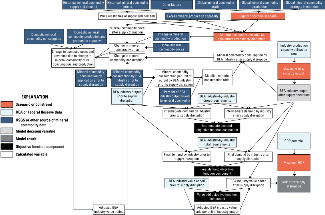
Diagram of a model for quantifying potential effects of mineral commodity supply disruptions on the U.S. economy. The diagram depicts the different data, constraints, and variables used in the model, as well as their sources and how they are interlinked. Bureau of Economic Analysis (BEA) data are from Bureau of Economic Analysis (2023); Federal Reserve data are from Board of Governors of the Federal Reserve System (2023). U.S. Geological Survey (USGS) data are from U.S. Geological Survey (undated). GDP, gross domestic product.
Data regarding mineral commodity production, production capacity, trade, inventories, and consumption for China, the United States, and the rest of the world were collected from a variety of sources (app. 1). All data pertain to 2021 or 2022, the latest years for which a complete set of IO tables and mineral commodity data were available before China’s export controls were established.
Given the lack of transparency in the gallium and germanium markets, a sensitivity analysis was performed in which each of the key parameters used in the model was varied to provide cases labeled as “low impact” and “high impact” in addition to the baseline case (app. 1). Finally, given that it is currently [2024] unclear how much (if any) of China’s net exports of gallium and germanium products will ultimately be restricted, the level of restriction was varied from 10 to 100 percent.
Results and Discussion
The price elasticities of demand for gallium and germanium were estimated to be −0.53 and −0.245, respectively. Meanwhile, the price elasticities of supply in the short run for gallium and germanium were estimated to be 0.40 and 0.69, respectively (app. 1). These elasticities suggest that the supply and demand for gallium and germanium were price inelastic, with absolute values falling between 0 and 1. The supply of germanium exhibited greater price elasticity compared with that of gallium, whereas the price elasticity of demand for germanium was lower (in absolute value) than that for gallium. It is important to highlight that the price elasticity of demand for gallium was derived from panel data within a static framework, potentially resulting in a larger absolute value compared to the short-run elasticity. In contrast, the price elasticity of demand for germanium was based on time-series data (app. 1), with the reported numbers reflecting short-run elasticity.
These price elasticities, along with data on China’s net exports and the rest of the world’s (excluding China) production, production capacity, consumption, and inventories, were used to estimate new equilibrium prices and quantities for the rest of the world under several different levels of supply disruption (as defined by the percentage of China’s net exports that were restricted). The results are displayed in figure 2.
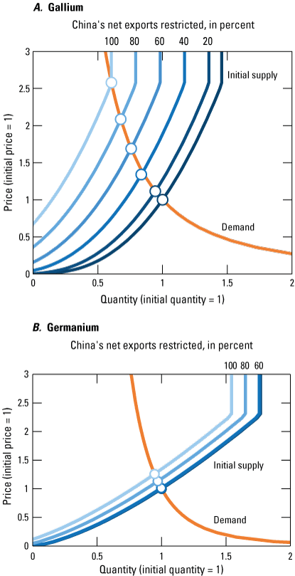
Estimated equilibrium quantities and prices for the rest of the world under different scenarios of Chinese net export restriction of A, gallium and B, germanium.
The results indicated that a complete restriction of China’s net exports of gallium, which were estimated to be 159 metric tons (t) out of a total world production of 638 t in 2022 (fig. 1.1; table 1.10), would cause gallium prices in the rest of the world to increase by more than 2.5-fold, while the quantity of gallium available to the rest of the world would decrease by about 39.5 percent. In contrast, a complete disruption of China’s net exports of germanium, which were estimated to be 35 t out of a total world production of 210 t in 2022 (tables 1.14 and 1.17), would cause germanium prices to increase by 26 percent and the quantity available to the rest of the world to decrease by about 5.5 percent. Less than complete restrictions of China’s net exports would result in correspondingly lower price increases and quantity decreases (fig. 2; app. 1). A complete restriction of China’s net exports of germanium has a lower effect than that of gallium due to the differences in price elasticities and the higher levels of germanium production, production capacity, and inventories in the rest of the world. Restriction of as much as 58 percent of China’s net exports of germanium could be offset by available inventories, thereby resulting in no shift in the supply curve.
The effects on the U.S. GDP at the level of individual industries and the economy overall were calculated using these relative shifts in quantities and prices in the IO model. The results (fig. 3) indicate that the U.S. GDP would decrease by $3.1 billion (or about 0.013 percent of U.S. GDP in 2021) if all of China’s net exports of gallium were restricted for an entire year. Nearly half (46.5 percent) of the decrease would come from the semiconductor and related device manufacturing industry (BEA industry code 334413)—the industry to which gallium consumption was directly linked to in the model. The remaining decrease would come from a wide assortment of industries, including several that are downstream from the 334413 industry, namely the printed circuit assembly (electronic assembly) manufacturing (334418), motor vehicle electrical and electronic equipment manufacturing (336320), and electronic computer manufacturing (334111). Notably, aside from the 334413 industry, no other individual industry dominated the decrease in U.S. GDP, and each industry’s relative contributions to the decrease remained largely consistent at different levels of restriction.
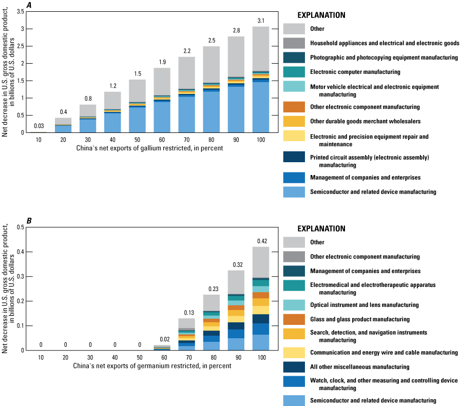
Estimated net decrease in U.S. gross domestic product at different levels of restrictions of China’s net exports of A, gallium or B, germanium, by industry.
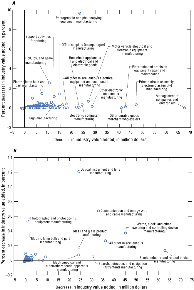
Scatterplots of absolute (horizonal axis) and relative (vertical axis) decrease of industry value added at 100 percent (%) restriction of China’s net exports of A, gallium and B, germanium. The semiconductor and related device manufacturing industry is not displayed in A due to horizonal axis truncation.
The decrease in U.S. GDP was estimated to be $0.4 billion under a scenario of complete restriction of China’s net exports of germanium. This was markedly lower than the decrease associated with the restriction of gallium primarily because the estimated decrease in equilibrium quantity was smaller, approximately 5.5 percent for germanium as compared to 39.5 percent for gallium. Therefore, excess production capacity and inventories in the rest of the world, which reduce the dependency on China, play an important role in reducing the effect of a germanium supply restriction.
Unlike the effect on the U.S. GDP from gallium restrictions, the effect on the U.S. GDP from germanium restrictions was not dominated by a single industry. Instead, the decrease was contributed to nearly evenly from several industries, with the largest contributions to the decrease coming from semiconductor and related device manufacturing (334413) and watch, clock, and other measuring and controlling device manufacturing (33451A; this is the industry that includes gamma-radiation detection equipment manufacturing that uses germanium). Although these were industries that were directly connected to germanium consumption in the model, they were not the largest direct consumers of germanium. The largest direct consumers of germanium were communication and energy wire and cable manufacturing (for fiber optic cables; 335920) and search, detection, and navigation instrument manufacturing (for infrared equipment; 334511). As before, restrictions of as much as 58 percent of China’s net exports of germanium were offset by available inventories.
Industries that contributed the most to the overall U.S. GDP decrease were not necessarily the industries that were most affected by the disruption. That is because some industries were larger contributors to GDP than others. The photographic and photocopying equipment manufacturing (333316) industry had the largest relative decrease in value added under a complete restriction of China’s net exports of gallium (fig. 4A). Other industries that had large relative decreases under this scenario were the doll, toy, and game manufacturing (339930), electric lamp bulb and part manufacturing (335110), and office supplies (except paper) manufacturing (339940) industries. For germanium (fig. 4B), the industry that had the largest relative decrease in value added was the optical instrument and lens manufacturing (333314). Again, this industry was not the largest consumer of germanium and did not have the largest absolute decrease in value added. Other industries that had large relative decreases in value added under this scenario were the communication and energy wire and cable manufacturing (335920), photographic and photocopying equipment manufacturing (333316), watch, clock, and other measuring and controlling device manufacturing (33451A), and electric lamp bulb and part manufacturing (335110) industries, all of which were directly linked to germanium consumption in the model.
Sensitivity Analysis
The results from the sensitivity analysis (fig. 5) illustrated the effects of varying key parameters (tables 1.10 and 1.26) on three results: changes in equilibrium quantities, prices, and U.S. GDP. Although not statistical confidence intervals, these results provide a window of likely ranges. For gallium, the results indicated that the decrease in U.S. GDP could be as high as $8.2 billion or as low as $1.7 billion. This relatively large range follows the change in equilibrium quantity but is somewhat more pronounced for the high-impact case at the highest levels of restrictions because of the notably higher prices and the higher percentage of the semiconductor and related device manufacturing industry that was assumed to use gallium. The lower and upper values of U.S. GDP decrease for germanium were estimated to be $0.01 billion and $1.1 billion, respectively. Again, these germanium results closely follow the change in equilibrium quantity.
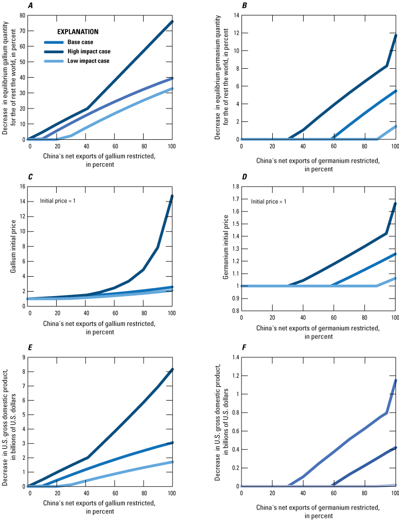
Sensitivity analysis displaying the effects of restricting (from 0 to 100 percent [%]) China's net exports of gallium and germanium on the A and B, rest of the world postdisruption equilibrium quantities, C and D, rest of the world postdisruption equilibrium prices, and E and F, U.S. gross domestic product (GDP) for the baseline, low-, and high-impact cases.
The change in slope for both the decrease in equilibrium quantity and U.S. GDP for gallium in the high-impact case occurs at a restriction of just over 41 percent of China’s net export. This was the point where the shift in the supply curve was large enough such that all the available excess production capacity was used (app. 1). That was the point where the demand curve intercepted the vertical portion of the supply curve, which resulted in larger increases in both changes in equilibrium quantities and prices at net export restrictions beyond that point. There was also a change in the slope in the result for gallium in the baseline case at a disruption level of 99.8 percent of China’s net exports due to the same reason (fig. 5A). This change in slope, however, did not occur for gallium in the low-impact case because the supply shift was small and the inventories and excess capacities in the rest of the world were larger. The change in slope only occurred for germanium in the high-impact case at a restriction of 94.1 percent of China’s net exports.
Comparison of Price and Quantity Effect
As described in the “Materials and Methods” section of this report and illustrated in equation 15, the modeled decrease in U.S. GDP is the result of two factors: decrease in industry output (to meet the mineral commodity availability constraint) and increase in mineral commodity prices. Both effects played a role in the results, but their contributions were not equal. When the model was simulated for the complete restriction of China’s net exports, higher prices only contributed 6.1 percent of the decrease in U.S. GDP for gallium and 2.2 percent of the decrease in U.S. GDP for germanium. These percentages were slightly lower at lower levels of China’s net export restriction and reached no higher than 12 to 16 percent in the results of the sensitivity analysis. These results suggested that the decrease in quantity available had far more of an effect on the decrease of the U.S. GDP than the increased prices, which is as might be expected given that the value of gallium- and germanium-containing devices (in other words, the value of the output of the industries) is notably greater than the cost of gallium and germanium raw materials. This may not be the case for all commodities because the ratio of the value of the commodities and the products that they are used in can vary markedly. It would also be dependent on the specific scenario and the price elasticities.
Simultaneous Disruptions
A complete and simultaneous restriction of China’s net exports of gallium and germanium was estimated to cause U.S. GDP to decrease by $3.4 billion ($1.7 billion to $9.0 billion for the low- and high-impact cases, respectively; fig. 6). The results from the simultaneous restrictions show the larger effect of gallium restrictions as compared to germanium restrictions. Furthermore, these decreases were slightly lower than the sum of the decreases from each mineral commodity when restricted individually. This was due to the interconnectedness of the affected industries (industries that would nominally be affected by the restriction of a commodity are also affected by the restriction of the other commodity and so their outputs do not decrease further). The effect on the U.S. GDP from the simultaneous disruption of both gallium and germanium would have been even lower than the sum of the effects from the restrictions on the individual commodities if some degree of concurrent uses among gallium and germanium were assumed. In contrast, one would expect the effect of simultaneous restrictions of mineral commodities that are used in notably distant sectors of the economy to have an effect that is closer to the sum of the effects of individual commodities.
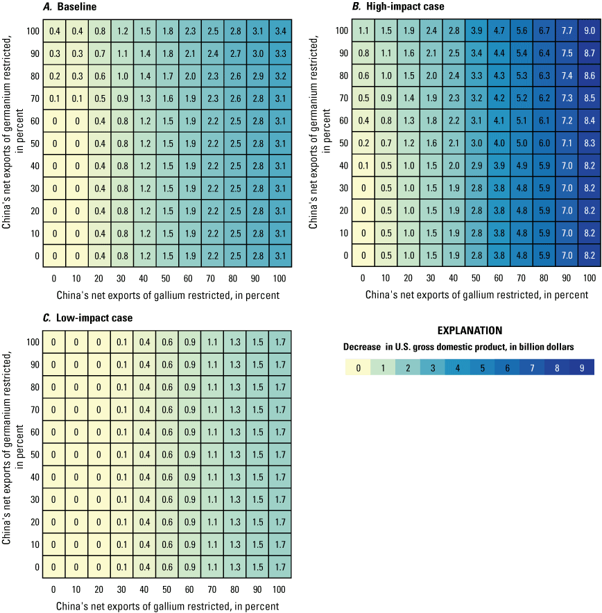
Heat maps displaying the estimated effects of simultaneous restrictions of China’s net exports (from 0 to 100 percent [%]) of gallium and germanium on the U.S. gross domestic product (GDP) for the A, baseline, B, low-, and C, high-impact cases of the sensitivity analysis.
Limitations and Applicability
As with all models, there were various limitations and assumptions within this model that a reader should be cognizant of while interpreting the results. Although many of the uncertainties associated with the various assumptions were addressed via the sensitivity analysis, some were inherent to the model. For example, although the assessment of price elasticity of demand captured short-term substitution effects for gallium and germanium, the model did not account for substitution effects among downstream industries due to the rigid structure of the IO tables. For example, gallium and germanium are used in wireless telecommunication technologies and fiberoptic cables, which are potential substitutes for each other in certain instances. Although the model determined which industries consumed the postdisruption available gallium and germanium, it did not account for the possibility of downstream industries or final consumers switching between the two telecommunication options. This, however, might be an acceptable assumption in the short term as such changes likely require longer periods to occur. The model also did not account for the effects of changes in gallium or germanium prices on the prices of their substitutes and their associated consuming industries and assumed constant elasticities and shifts in the supply curves when calculating the new equilibriums.
Another simplifying assumption was that the different forms of gallium and germanium were interchangeable. That may not be the case as there may be limits to production capacities for certain forms (for example, reduction of an oxide to a metal or the production of high-purity single crystals). As discussed in the “Materials and Methods” section of this report, another limitation was that, even at the detailed level, the IO tables were not granular enough for some of the niche uses of these minor elements. The modified material consumption ratio addressed this issue by affecting only a portion of the consuming industry’s output. However, this approach implicitly assumed that the mix of downstream industries and final consumers for this niche use was not different from the industry overall. If this were not the case, then the downstream industries that would be affected from the supply restriction would be different from what was modeled. The model also assumed that industries and final consumers want to return to their original consumption patterns, which might not always be the case, especially in the long term. There were also inherent assumptions regarding which industries gallium and germanium consumption were linked to in the model. Additionally, this analysis was specific to the disruption of gallium and germanium metals, compounds, and wafers and not the devices and products that contain these mineral commodities. Therefore, the results do not account for any disruptions in the availability of such downstream devices and finished products that were produced outside of the United States that may no longer be available for trade due to China restricting exports of the raw materials.
Despite these limitations, the results presented here provide an assessment that could be useful in making decisions regarding various mitigation strategies. For example, with the results from this analysis, a cost-benefit analysis can be performed to determine levels of maintaining or expanding strategic inventories. Similarly, plans for new plants to recover gallium and germanium can be assessed on a quantitative basis. This is noteworthy given that most of the gallium and germanium present in mined ores are not currently recovered (Licht and others, 2015; Frenzel and others, 2016, 2017). Similarly, while significant amounts of gallium and germanium are recycled as new scrap during fabrication and manufacturing, there is very limited postconsumer or end-of-life recycling of either element (Graedel and others, 2011; Licht and others, 2015; Mir and others, 2022). There is thus great potential for increasing and diversifying supplies, with several new sources of gallium and germanium being proposed or developed. For example, in late 2023, a newly built hydrometallurgical facility in southeastern Democratic Republic of the Congo noted that it had the capability of providing 30 percent of global germanium supply from processed slag (Société congolaise pour le traitement du terril de Lubumbashi, [undated]), although it was unclear if any production had taken place. Domestically, a zinc smelter in Clarksville, Tennessee, which already produces a germanium concentrate for export, was assessing the feasibility of a $150 million project to recover what it believes would be as much as 80 percent of annual U.S. consumption of gallium and germanium (Nyrstar, 2024). This model can be used to analyze various policies or incentives against the risks or costs of inaction for specific projects. Furthermore, when extended to include other mineral commodities, this analysis could be used to determine the U.S. list of critical minerals (Nassar and Fortier, 2021), which is a U.S. government-wide prioritized list of commodities of most concern that has provided the basis for various actions and policies, such as the Infrastructure Investment and Jobs Act of 2021 (Public Law 117–58; 135 Stat. 429) and the Inflation Reduction Act of 2022 (Public Law 117–169; 136 Stat. 1818).
References Cited
Bauer, D., Khazdozian, H., Mehta, J., Nguyen, R.T., Severson, M.H., Vaagensmith, B.C., Toba, L., Zhang, B., Hossain, T., Sibal, A.P., Smith, B.J., Riddle, M.E., Graziano, D.J., Mathew, T., Cuscaden, P., Dai, Q., Iloeje, C., Edgemon, L., Sarna, C., and Quaresima, J., 2023, Critical materials assessment: U.S. Department of Energy DE–AC07–05ID14517, 240 p., accessed July 30, 2024, at https://inldigitallibrary.inl.gov/sites/sti/sti/Sort_66849.pdf.
Board of Governors of the Federal Reserve System, 2023, Industrial production and capacity utilization—G.17: Board of Governors of the Federal Reserve System data, accessed August 11, 2023, at https://www.federalreserve.gov/releases/g17/caputl.htm.
Bureau of Economic Analysis, 2023, GDP by industry: U.S. Bureau of Economic Analysis interactive data tables, accessed July 30, 2024, at https://www.bea.gov/itable/gdp-by-industry.
Congressional Budget Office, 2024, Real potential gross domestic product [GDPPOT]: Congressional Budget Office data, accessed July 30, 2024, at https://fred.stlouisfed.org/series/GDPPOT.
Feldman, D., Zuboy, J., Dummit, K., Stright, D., Heine, M., Mirletz, H., and Margolis, R., 2024, Winter 2024 solar industry update: National Renewable Energy Laboratory, 60 p., accessed July 30, 2024, at https://www.nrel.gov/docs/fy24osti/88780.pdf.
Frenzel, M., Ketris, M.P., Seifert, T., and Gutzmer, J., 2016, On the current and future availability of gallium: Resources Policy, v. 47, p. 38–50, accessed July 30, 2024, at https://doi.org/10.1016/j.resourpol.2015.11.005.
Frenzel, M., Mikolajczak, C., Reuter, M.A., and Gutzmer, J., 2017, Quantifying the relative availability of high-tech by-product metals—The cases of gallium, germanium and indium: Resources Policy, v. 52, p. 327–335, accessed July 30, 2024, at https://doi.org/10.1016/j.resourpol.2017.04.008.
Ghosh, A., 1958, Input-output approach in an allocation system: Economica, v. 25, no. 97, p. 58–64, accessed July 30, 2024, at https://doi.org/10.2307/2550694.
Graedel, T.E., Allwood, J., Birat, J.-P., Buchert, M., Hageluken, C., Reck, B.K., Sibley, S.F., and Sonnemann, G., 2011, What do we know about metal recycling rates?: Journal of Industrial Ecology, v. 15, no. 3, p. 355–366, accessed July 30, 2024, at https://doi.org/10.1111/j.1530-9290.2011.00342.x.
Graedel, T.E., Harper, E.M., Nassar, N.T., Nuss, P., and Reck, B.K., 2015, Criticality of metals and metalloids: Proceedings of the National Academy of Sciences of the United States of America, v. 112, no. 14, p. 4257–4262, accessed July 30, 2024, at https://doi.org/10.1073/pnas.1500415112.
Grohol, M., and Veeh, C., 2023, Study on the critical raw materials for the EU—2023—Final report: European Commission Directorate-General for Internal Market, Industry, Entrepreneurship and SMEs, 152 p., accessed July 30, 2024, at https://doi.org/10.2873/725585.
Guberman, D.E., 2010–16, Germanium, in Metals and minerals: U.S. Geological Survey Minerals Yearbook 2007–14, v. I, chap. 30, [variously paginated], accessed July 30, 2024, at https://www.usgs.gov/centers/national-minerals-information-center/germanium-statistics-and-information.
Guberman, D.E., and Thomas, C.L., 2017, Germanium, in Metals and minerals: U.S. Geological Survey Minerals Yearbook 2015, v. I, chap. 30, p. 30.1–30.7, accessed July 30, 2024, at https://www.usgs.gov/centers/national-minerals-information-center/germanium-statistics-and-information.
Gulley, A.L., Nassar, N.T., and Xun, S., 2018, China, the United States, and competition for resources that enable emerging technologies: Proceedings of the National Academy of Sciences of the United States of America, v. 115, no. 16, p. 4111–4115, accessed July 30, 2024, at https://doi.org/10.1073/PNAS.1717152115.
Horowitz, K.J., and Planting, M.A., 2006, Concepts and methods of the input-output accounts [updated April 2009]: Bureau of Economic Analysis, 266 p., accessed July 30, 2024, at https://www.bea.gov/sites/default/files/methodologies/IOmanual_092906.pdf.
Jaskula, B.W., 2010–23, Gallium, in Metals and minerals: U.S. Geological Survey Minerals Yearbook 2007–21, v. I, chap. 27, [variously paginated], accessed July 30, 2024, at https://www.usgs.gov/centers/national-minerals-information-center/gallium-statistics-and-information.
Jowitt, S.M., 2020, Covid-19 and the global mining industry: SEG Discovery, v. 122, p. 33–41, accessed July 30, 2024, at https://doi.org/10.5382/SEGnews.2020-122.fea-02.
Kalantzakos, S., 2020, The race for critical minerals in an era of geopolitical realignments: The International Spectator, v. 55, no. 3, p. 1–16, accessed July 30, 2024, at https://doi.org/10.1080/03932729.2020.1786926.
Khurshid, A., Chen, Y., Rauf, A., and Khan, K., 2023, Critical metals in uncertainty—How Russia-Ukraine conflict drives their prices?: Resources Policy, v. 85, part B, August, article 104000, 10 p., accessed July 30, 2024, at https://doi.org/10.1016/j.resourpol.2023.104000.
Ku, A.Y., Loudis, J., and Duclos, S.J., 2018, The impact of technological innovation on critical materials risk dynamics: Sustainable Material Technology, v. 15, p. 19–26, accessed July 30, 2024, at https://doi.org/10.1016/j.susmat.2017.11.002.
Li, M., Lenzen, M., Pedauga, L.E., and Malik, A., 2022, A minimum-disruption approach to input-output disaster analysis: Spatial Economic Analysis, v. 17, no. 4, p. 446–470, accessed July 30, 2024, at https://doi.org/10.1080/17421772.2022.2056231.
Licht, C., Peiró, L.T., and Villalba, G., 2015, Global substance flow analysis of gallium, germanium, and indium—Quantification of extraction, uses, and dissipative losses within their anthropogenic cycles: Journal of Industrial Ecology, v. 19, no. 5, p. 890–903, accessed July 30, 2024, at https://doi.org/10.1111/jiec.12287.
Løvik, A.N., Restrepo, E., and Müller, D.B., 2015, The global anthropogenic gallium system—Determinants of demand, supply and efficiency improvements: Environmental Science and Technology, v. 49, no. 9, p. 5704–5712, accessed July 30, 2024, at https://doi.org/10.1021/acs.est.5b00320.
Manley, R.L., Alonso, E., and Nassar, N.T., 2022a, A model to assess industry vulnerability to disruptions in mineral commodity supplies: Resources Policy, v. 78, September, article 102889, p., accessed July 30, 2024, at https://doi.org/10.1016/j.resourpol.2022.102889.
Manley, R.L., Alonso, E., and Nassar, N.T., 2022b, Examining industry vulnerability—A focus on mineral commodities used in the automotive and electronics industries: Resources Policy, v. 78, September, article 102894, 8 p., accessed July 30, 2024, at https://doi.org/10.1016/j.resourpol.2022.102894.
Ministry of Commerce and General Administration of Customs [China], 2023, Implementation of export controls on gallium and germanium related items [in Chinese]: Ministry of Commerce and General Administration of Customs announcement 23, accessed October 2, 2023, at http://www.mofcom.gov.cn/article/zwgk/gkzcfb/202307/20230703419666.shtml.
Mir, S., Vaishampayan, A., and Dhawan, N., 2022, A review on recycling of end-of-life light-emitting diodes for metal recovery: Journal of the Minerals Metals & Materials Society [JOM], v. 74, p. 599–611, accessed July 30, 2024, at https://doi.org/10.1007/s11837-021-05043-9.
Nassar, N.T., 2023, Minerals for a changing world: Elements, v. 19, p. 342–344, accessed August 15, 2024, at https://doi.org/10.2138/gselements.19.6.342.
Nassar, N.T., and Fortier, S.M., 2021, Methodology and technical input for the 2021 review and revision of the U.S. critical minerals list: U.S. Geological Survey Open-File Report 2021–1045, 31 p., accessed July 30, 2024, at https://doi.org/10.3133/ofr20211045.
Nassar, N.T., Alonso, E., and Brainard, J., 2020a, Investigation of U.S. foreign reliance on critical minerals—U.S. Geological Survey technical input document in response to Executive Order No. 13953 signed September 30: U.S. Geological Survey Open-File Report 2020–1127, 37 p., accessed July 30, 2024, at https://doi.org/10.3133/ofr20201127.
Nassar, N.T., Brainard, J., Gulley, A., Manley, R., Matos, G., Lederer, G., Bird, L.R., Pineault, D., Alonso, E., Gambogi, J., and Fortier, S.M., 2020b, Evaluating the mineral commodity supply risk of the U.S. manufacturing sector: Science Advances, v. 6, no. 8, article eaay8647, 11 p., accessed July 30, 2024, at https://doi.org/10.1126/sciadv.aay8647.
Nassar, N.T., Graedel, T.E., and Harper, E.M., 2015, By-product metals are technologically essential but have problematic supply: Science Advances, v. 1, no. 3, article e1400180, 10 p., accessed July 30, 2024, at https://doi.org/10.1126/sciadv.1400180.
National Research Council, 2008, Minerals, critical minerals, and the U.S. economy: The National Academy of Sciences report, prepared by the National Research Council, 246 p., accessed July 30, 2024, at https://nap.nationalacademies.org/catalog/12034/minerals-critical-minerals-and-the-us-economy.
Nyrstar, 2024, Nyrstar Clarksville: Nyrstar web page, accessed July 30, 2024, at https://www.nyrstar.com/operations/metals-processing/nyrstar-clarksville.
Oosterhaven, J., 1988, On the plausibility of the supply-driven input-output model: Journal of Regional Science, v. 28, no. 2, p. 203–217, accessed July 30, 2024, at https://doi.org/10.1111/j.1467-9787.1988.tb01208.x.
Oosterhaven, J., 2017, On the limited usability of the inoperability IO model: Economic Systems Research, v. 29, no. 3, p. 452–461, accessed July 30, 2024, at https://doi.org/10.1080/09535314.2017.1301395.
Oosterhaven, J., and Bouwmeester, M.C., 2016, A new approach to modeling the impact of disruptive events: Journal of Regional Science, v. 56, no. 4, p. 583–595, accessed July 30, 2024, at https://doi.org/10.1111/jors.12262.
Prajapati, P., and Balamurugan, S., 2023, Leveraging GaN for DC–DC power modules for efficient EVs—A review: IEEE Access : Practical Innovations, Open Solutions, v. 11, p. 95874–95888, accessed July 30, 2024, at https://doi.org/10.1109/ACCESS.2023.3311266.
Project Blue Group Ltd., 2023, Gallium market service: Project Blue Group Ltd. web page, accessed July 30, 2024, at https://projectblue.com/subscriptions/critical-materials/gallium.
Schrijvers, D., Hool, A., Blengini, G.A., Chen, W.-Q., Dewulf, J., Eggert, R., van Ellen, L., Gauss, R., Goddin, J., Habib, K., Hagelüken, C., Hirohata, A., Hofmann-Amtenbrink, M., Kosmol, J., Le Gleuher, M., Grohol, M., Ku, A., Lee, M.-H., Liu, G., Nansai, K., Nuss, P., Peck, D., Reller, A., Sonnemann, G., Tercero., L., Thorenz, A., and Wäger, P.A., 2020, A review of methods and data to determine raw material criticality: Resources, Conservation & Recycling, v. 155, April, article 104617, 17 p., accessed July 30, 2024, at https://doi.org/10.1016/j.resconrec.2019.104617.
Shojaeddini, E., Alonso, E., and Nassar, N.T., 2024, Estimating price elasticity of demand for mineral commodities used in lithium-ion batteries in the face of surging demand: Resources Conservation Recycling, v. 207, August, article 107664, 9 p., accessed July 30, 2024, at https://doi.org/10.1016/j.resconrec.2024.107664.
Société congolaise pour le traitement du terril de Lubumbashi, [undated], STL—Home: Société congolaise pour le traitement du terril de Lubumbashi web page, accessed July 30, 2024, at https://www.stlgcm.com/.
Thomas, C.L., 2018–23, Germanium, in Metals and minerals: U.S. Geological Survey Minerals Yearbook 2016–19, v. I, chap. 30, [variously paginated], accessed July 30, 2024, at https://www.usgs.gov/centers/national-minerals-information-center/germanium-statistics-and-information.
U.S. Census Bureau, 2022, 2018–2021 annual survey of manufactures (ASM)—Tables: U.S. Census Bureau data, accessed October 11, 2023, at https://www.census.gov/data/tables/time-series/econ/asm/2018-2021-asm.html.
U.S. Census Bureau, 2023, 2017 NAICS sector 31-33—Manufacturing: U.S. Census Bureau data, accessed December 5, 2023, at https://www.census.gov/data/tables/2017/econ/economic-census/naics-sector-31-33.html.
U.S. Geological Survey, 2008–24, Mineral commodity summaries 2008–24: U.S. Geological Survey, accessed July 30, 2024, at https://www.usgs.gov/centers/national-minerals-information-center/mineral-commodity-summaries.
U.S. Geological Survey, [undated], Commodity statistics and information: U.S. Geological Survey National Minerals Information Center web page, accessed August 26, 2024, at https://www.usgs.gov/centers/national-minerals-information-center/commodity-statistics-and-information.
Yole Développement, 2018, GaAs wafer and epiwafer market—RF, photonics, LED, and PV applications 2020: Yole Développement market and technology report, accessed July 30, 2024, at https://www.everythingrf.com/research-reports/details/47-gaas-wafer-and-epiwafer-market-rf-photonics-led-display-and-pv-applications-2020.
Yole Développement, 2020, GaN RF market—Applications, players, technology and substrates—Forecast period 2019–2025: Yole Développement market and technology report, accessed July 30, 2024, at https://www.everythingrf.com/research-reports/details/40-gan-rf-market-applications-players-technology-and-substrates-2020.
Appendix 1. Supplemental Information for Quantifying Potential Effects of China’s Gallium and Germanium Export Restrictions on the U.S. Economy
Estimating Postdisruption Equilibrium Quantities and Prices
To determine equilibrium quantities and prices after a disruption, by using price elasticities of supply and demand, two basic log-linear supply (eq. 1.1) and demand (eq. 1.2) equations were used, as follows:
where S and D refer to the supply and demand respectively, Q refers to quantity, P refers to price, ε refers to price elasticity, and α and β are terms that account for all other variables that affect supply and demand, respectively.At initial equilibrium, before the disruption, the following was obtained:
A constant supply shift of magnitude (ΔQS) or relative magnitude (nS) can be defined as follows, where the shifted supply curve is :
Similarly, a constant demand shift of magnitude (ΔQD) or relative magnitude (nD) can be defined as follows, where the shifted demand curve is :
These supply and demand shifts were provided exogenously based on the scenario being examined and were assessed after accounting for available inventories that abated some or all the disruptions (for example, the inventory-adjusted shift in supply was the initial shift less any inventory releases). With these shifts in the supply and demand curves, the new equilibrium price (P′) was determined, as follows:
This nonlinear relation among price elasticities, price ratios, and relative shifts in the supply and demand curves was solved empirically to determine the new equilibrium price.With the new equilibrium price, the change in quantity from the initial equilibrium to the new equilibrium on an absolute (ΔQ′) and a relative (n′) basis was determined by using the demand curve, as follows:
The relative change in quantity from the initial to the new equilibrium quantity can also be determined in terms of the supply curve using the same approach:An assumption in the above derivation was that the price elasticity of supply is constant and that there was sufficient excess production capacity. However, that assumption was modified by noting that there was finite excess production capacity (κ), after which supply could not be increased regardless of the commodity’s price. On the predisruption supply curve, this would occur at a certain price (P*) at which all excess capacity would have been used, as follows:
The quantity (Q*) that this price would yield on the shifted demand curve was determined, as follows: The relative change in quantity necessary to get to this point () was defined as follows: Therefore, if , then the new equilibrium quantity became the initial equilibrium quantity plus all the excess capacity less the amount that was disrupted: This new quantity was set equal to the shifted demand curve to find the new equilibrium price: Using the new equilibrium price, the relative quantity shift to the new equilibrium (n′) was calculated by using equation 1.21: Note that the difference between n′ and nS represents the relative quantity of the excess production capacity that was utilized postdisruption (κu), which can be obtained from equation 1.22 or 1.34. Also note that, if there was no shift in the demand curve and if , then the new equilibrium price simplifies to:Empirical estimation of price elasticities.—Two general approaches to estimate the price elasticity of demand and price elasticity of supply for gallium and germanium were used. First, for the price elasticity of demand estimate with panel data, the demand elasticities were estimated by using a static framework, because the data used in the analysis lack a sufficiently long-time dimension to employ dynamic models. To tackle potential simultaneity issues of the price and consumption/production variables, a two-stage least-square and instrumental variable approach was employed. Following Shojaeddini and others (2024), the two-stage least-square regression was as follows:
In the first stage, the mineral commodity price (p) at time t and within sector i was determined through a function incorporating instrumental variable (Z) and other control variables (X). Subsequently, in the second stage, the estimation of the quantity demanded (d) for the mineral commodity involved utilizing the forecasted price () from the first stage alongside additional control variables. To facilitate the analysis, the variables were transformed logarithmically, allowing the estimated price coefficient (ε) to offer insights into the price elasticity of demand. Constants α0 and β0 denoted general terms, and αi and βi represented sector-specific constant terms referred to as sector-level fixed effects. Parameters αj and ακ denoted the impacts of control variables and instrumental variables on commodity price, respectively, while βj represented the influence of control variables on commodity demand. Furthermore, the terms vt and et served as error components in the model.
For the estimation of the price elasticities with time series data, an autoregressive distributed lag model was employed. This model estimates the production or consumption variable on its own lagged values, as well as on the current and lagged values of other control variables. Following Pesaran and Shin (1999) and Pesaran and others (2001), an autoregressive distributed lag (ρ, h1, h2, …, hn) model has the following general form:
where qt represented the commodity’s production or consumption quantity for year t; X was a vector of other explanatory variables, including the commodity’s price; ρ represented the lag order for the dependent variable; h was the lag order for other variables that was not necessarily the same for each explanatory variable (n); and ω and β′ were the corresponding coefficients for q and X, respectively.The error correction version of the autoregressive distributed lag model was represented by the following:
where Δ was the first difference, ECT = [qt−1 – λ′Xt−1] was the error correction term, and θ was the speed of adjustment coefficient. The first part of the equation with θ and λ represented the long-run relationship, and the second part with ω and β represented the short-run dynamics of the model. Due to potential simultaneity issues, the autoregressive distributed lag model was estimated in two stages using an instrumental variable approach as previously described.A structural break test (Ditzen and others, 2021) was used to examine whether there have been changes in the model parameters from significant disruptive events and to determine when these changes occurred. An interaction term was introduced between the price variable and a binary variable to indicate the occurrence of the structural change. By integrating this interaction term, which links the mineral commodity price variable with a binary variable reflecting the identified structural break in the market, the price elasticity of demand and price elasticity of supply variance before and after the structural break were evaluated. If the interaction term proved statistically insignificant in certain instances, the binary variable was incorporated into the regression to ensure parameter stability.
The price elasticity of demand of gallium was estimated by using global consumption data by each application sector obtained from Project Blue Group Ltd. (2023), and of germanium, from U.S. apparent consumption data from the U.S. Geological Survey (USGS; Kelly and Matos, 2023; Thomas, 2023; U.S. Geological Survey, 2024). The price elasticity of supply was estimated using the worldwide time series of primary production for each commodity (Jaskula, 2021; Kelly and Matos, 2023; Thomas, 2023; U.S. Geological Survey, 2024).
Gallium prices were derived from the average unit value of U.S. imports for low-purity gallium (U.S. Geological Survey, 2024). Germanium prices were from U.S. Geological Survey (2013, 2024) and reflected the average price of germanium metal (more than or equal to 99.99 percent) and unit value of U.S. imports.
For explanatory variables, the industrial production index for U.S. manufacturing was obtained from Board of Governors of the Federal Reserve System (2024). Silicon metal prices, bauxite, zinc, and coal production were from U.S. Geological Survey (2013, 2024). The results are summarized in tables 1.1 through 1.4. Each set of columns represents results derived from either a different estimation method or a different set of variables.
Table 1.1.
Estimation of price elasticity of demand of gallium.[The regression includes sector identification variables, which are binary variables representing each demand sector. Significance levels are denoted as *** (p-value<0.01), ** (p-value <0.05), and * (p-value <0.1). All monetary variables are adjusted for inflation using the world gross domestic product (GDP) deflator. GDP deflator is calculated using data from the World Bank Group, specifically world GDP constant in 2015 U.S. dollars purchasing power equivalent (World Bank Group, 2023a) and world GDP in current U.S. dollars (World Bank Group, 2023b). This deflator represents the global inflation rate, providing a measure of how much prices have increased on average across the world economy. SE, bootstrapped/heteroskedasticity and autocorrelation robust standard error; Ga, gallium; Si, silicon; LED, light-emitting diode; 2SLS, two-stage least squares estimation]
| Variable | Log(Ga consumption) | |
|---|---|---|
| Coefficient | SE | |
| Log(Ga real price) | −0.53* | 0.31 |
| LED penetration rate | 0.02*** | 0.00 |
| Log(Si metal real price) | 0.47* | 0.26 |
| Constant | 4.82*** | 0.67 |
| Number of observations | 50 | |
| Estimation method | 2SLS | |
| Ga price data basis (source) | Low-purity, primary gallium ore (U.S. Geological Survey, 2024) | |
| Instrumental variable | Bauxite production | |
| Adjusted coefficient of determination (R2) | 0.942 | |
| Weak identification test p-value | 0.001 | |
Table 1.2.
Estimation of price elasticity of supply of gallium.[The regression includes sector identification variables, which are binary variables representing each demand sector. Significance levels are denoted as *** (p-value<0.01), ** (p-value <0.05), and * (p-value <0.1). All monetary variables are adjusted for inflation using the world gross domestic product (GDP) deflator. GDP deflator is calculated using data from the World Bank Group, specifically world GDP constant in 2015 U.S. dollars purchasing power equivalent (World Bank Group, 2023a) and world GDP in current U.S. dollars (World Bank Group, 2023b). This deflator represents the global inflation rate, providing a measure of how much prices have increased on average across the world economy. Gallium price represents low purity gallium for recent years which has been extrapolated back using gallium average price (99.9999-percent-pure metal) from 1959 to 2000. Variables beginning with “Dum” (short for dummy) signify binary variables. They take the value of 1 after the year indicated following “Dum” in the variable’s name and remain at 0 otherwise. SE, bootstrapped/heteroskedasticity and autocorrelation robust standard error; Ga, gallium; Si, silicon; 2SLS, two-stage least squares estimation; ARDL, autoregressive distributed lag model; —, not applicable; t−1, previous year]
Table 1.3.
Germanium price elasticity of demand estimation.[The regression includes sector identification variables, which are binary variables representing each demand sector. Significance levels are denoted as *** (p-value<0.01), ** (p-value <0.05), and * (p-value <0.1). All monetary variables are adjusted for inflation using the world gross domestic product (GDP) deflator. GDP deflator is calculated using data from the World Bank Group, specifically world GDP constant in 2015 U.S. dollars purchasing power equivalent (World Bank Group, 2023a) and world GDP in current U.S. dollars (World Bank Group, 2023b). This deflator represents the global inflation rate, providing a measure of how much prices have increased on average across the world economy. SE, bootstrapped/heteroskedasticity and autocorrelation robust standard error; Ge, germanium; Si, silicon; 2SLS, two-stage least squares estimation; ARDL, autoregressive distributed lag model; t−1, previous year]
Table 1.4.
Germanium price elasticity of supply estimation.[The regression includes sector identification variables, which are binary variables representing each demand sector. Significance levels are denoted as *** (p-value<0.01), ** (p-value <0.05), and * (p-value <0.1). All monetary variables are adjusted for inflation using the world gross domestic product (GDP) deflator. GDP deflator is calculated using data from the World Bank Group, specifically world GDP constant in 2015 U.S. dollars purchasing power equivalent (World Bank Group, 2023a) and world GDP in current U.S. dollars (World Bank Group, 2023b). This deflator represents the global inflation rate, providing a measure of how much prices have increased on average across the world economy. Variables beginning with “Dum” (short for dummy) signify binary variables. They take the value of 1 after the year indicated following “Dum” in the variable’s name and remain at 0 otherwise. The interaction between the price variable and the binary variable shows changes in the price elasticity of demand following the specified year indicated by the structural break year. SE, bootstrapped/heteroskedasticity and autocorrelation robust standard error; Ge, germanium; Si, silicon; 2SLS, two-stage least squares estimation; ARDL, autoregressive distributed lag model; —, not applicable; t−1, previous year]
Gallium
World Production and Production Capacity
In addition to primary (low purity; figs. 1.1, 1.2, and 1.3) gallium production and production capacities, refined (high purity) and secondary (new scrap recycled) gallium production and production capacities were reported or estimated based on various sources (table 1.5).
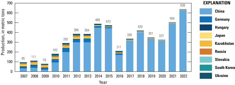
Graph showing world production of primary (low-purity) gallium, by country, from 2007 to 2022. Data are from Jaskula (2021) and U.S. Geological Survey (2024), with updated numbers for China from Asian Metals Ltd. (2023a).
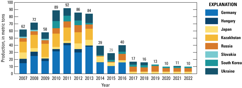
Graph showing production of primary (low-purity) gallium outside of China from 2007 to 2022. Data are from Jaskula (2021) and U.S. Geological Survey (2024).
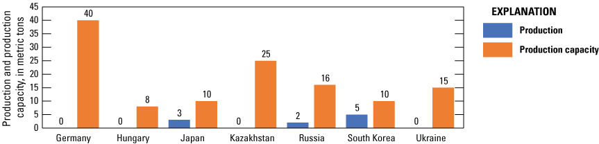
Graph showing production and production capacity of primary (low-purity) gallium outside of China, in 2022. Data are from Jaskula (2021) and U.S. Geological Survey (2024).
Table 1.5.
Primary (low purity), primary (high purity) refined, and secondary refined production and production capacities by country, circa 2021/2022[Data are from Rongguo and others (2016), Roskill Information Services Ltd. (2020), Jaskula (2021), Asian Metals Ltd. (2023a), Neo Performance Materials (2023), Project Blue Group Ltd. (2023), Japan Organization for Metals and Energy Security (2024), U.S. Geological Survey (2024), or estimated by the authors using trade data (Zen Innovations AG (2024)). t, metric ton]
China’s Trade of Gallium Products
China’s Ministry of Commerce announced on July 3, 2023 (Ministry of Commerce and General Administration of Customs [China], 2023), the export controls on eight gallium products, which fall under several 10-digit Harmonized Commodity Description and Coding System (HS) codes (table 1.6).
Table 1.6.
Harmonized System codes for gallium products with recent export controls by China.[Harmonized Commodity Description and Coding System (HS) codes are from Ministry of Commerce and General Administration of Customs [China], 2023]
Trade data are only available at the 8-digit HS codes. Therefore, trade of gallium under most of these codes is obscured because they include other products that do not contain gallium. Specifically, only trade data for gallium metal (HS codes 8112.9290 and 8112.9990) are directly discernable in the data reported by China (figs. 1.4–1.9). A few countries, however, report trade with China for gallium-arsenide (GaAs) wafers (table 1.7).
Graph showing China’s exports of gallium unwrought metal (Harmonized Schedule code 8112.9290), as reported by China, from 2007 to 2023. Data are from Zen Innovations AG (2024).
Graph showing China’s exports of gallium wrought metal (Harmonized Schedule code 8112.9990), as reported by China, from 2007 to 2023. Data are from Zen Innovations AG (2024).
Graph showing China’s exports of gallium-arsenide (GaAs) wafers (gallium content), as reported by trade partner (mirror trade), from 2007 to 2023. Low-value exports (less than $200 per kilogram) are assumed to be low-quality GaAs scrap or sludge and thus excluded. U.S. trade data were obtained at the district level. Data are from Zen Innovations AG (2024).
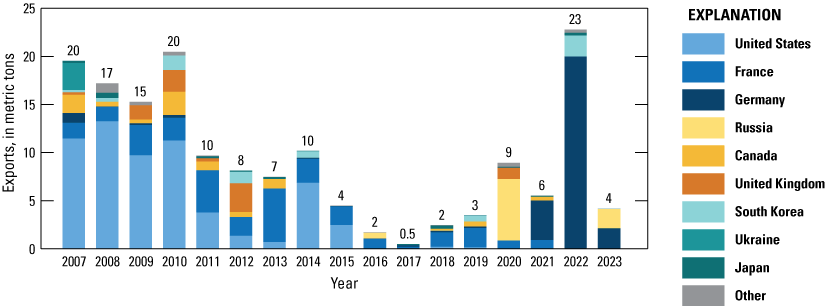
Graph showing China’s imports of gallium unwrought metal (Harmonized Schedule code 8112.92.90), as reported by China, from 2007 to 2023. Data are from Zen Innovations AG (2024).
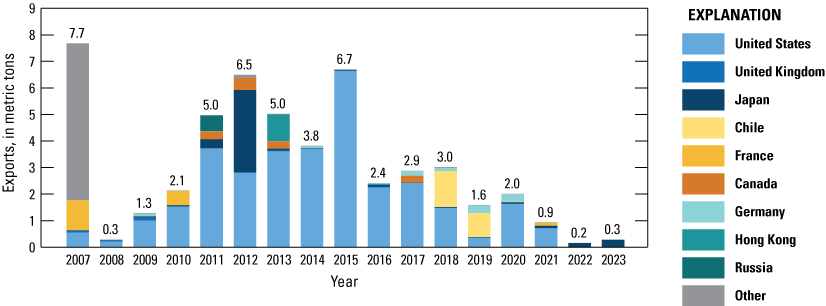
Graph showing China’s imports of gallium wrought metal (Harmonized Schedule code 8112.99.90) as reported by China, from 2007 to 2023. Data are from Zen Innovations AG (2024).
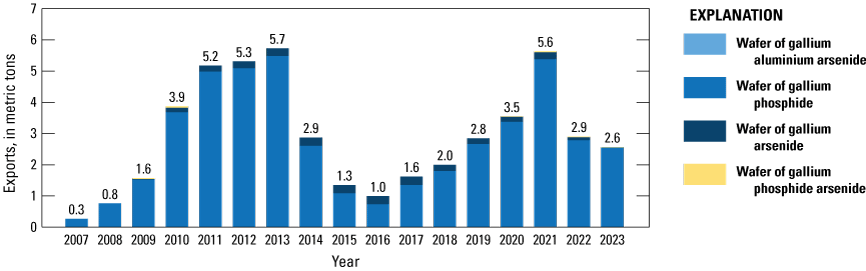
Graph showing China’s imports of gallium-containing wafers (estimated gallium content), as reported by Taiwan (mirror trade), from 2007 to 2023; Taiwan is the only country to report shipping gallium-containing wafers to China. Data are from Zen Innovations AG (2024).
Table 1.7.
Summary of China’s trade of gallium metal and gallium-containing wafers for 2021 to 2023.[Values may not add to totals shown due to rounding. HS, Harmonized Schedule code, from Ministry of Commerce and General Administration of Customs [China] (2023)]
Simplified Gallium Material Flow and Trade Analysis
To estimate the trade flows of gallium that were undifferentiable from the trade data, a simplified material flow diagram was developed for two regions: China and the rest of the world. The known production quantities for low-purity, high-purity refined, and secondary production (table 1.8) were assumed to be fixed. Trade flows for high-purity refined metal that were exported from the rest of the world to China and trade of gallium-containing wafers were all assumed to be accounted for in the trade data and that there were no significant changes in inventories in the rest of the world. Finally, data were obtained from Løvik and others (2015) on yield at fabrication, recycling collection rate, and recycling efficiency. The imports of low-purity gallium and scrap by the rest of the world from China were then estimated based on mass balance (fig. 1.10).
Table 1.8.
Summary of U.S. trade data of gallium for 2021–23.[Values may not add to totals shown due to rounding. GaAs, gallium arsenide]
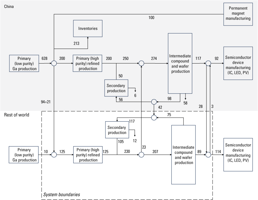
Simplified material flow and trade analysis for gallium flows between China and the rest of the world in 2022. Boxes represent transformative processes (for example, refining); circles represent distributive processes (such as international trade); and arrows represent material flows. Arrows that do not connect boxes and circles are process losses. Quantities are in metric tons of contained gallium but may not add to totals shown due to rounding.
Based on this mass balance analysis, an additional 21 metric tons (t) of low-purity primary gallium, above the 94 t that was identified by the gallium-distinguishable trade data, seems to have been exported from China to the rest of the world in 2022. Similarly, an additional 42 t of gallium contained in new (preconsumer) scrap seems to have been exported from China to the rest of the world. Across all forms, China’s exports to and imports from the rest of the world summed to 185 t and 26 t of contained gallium, respectively, resulting in estimated net exports of 159 t in 2022.
Gallium Inventories Outside of China
As indicated in the material flow analysis (fig. 1.10), there were notable flows to inventory from China’s production; these were calculated as the differences between the China’s primary low-purity production and the sum of China’s high-purity production, net exports of low-purity to the rest of the world, and China’s use of gallium in neodymium-iron-boron (NdFeB) permanent magnets, with the latter being estimated based on data in the literature (Project Blue Group Ltd., 2023). The quantity of gallium held in inventories outside of China is not generally known. However, the amount that might be available was estimated, as follows: In 2022, consumer inventories in the United States were reportedly 2.78 t of contained gallium (U.S. Geological Survey, 2024). Although no data on inventories were reported, Japan’s government announced that it was looking to maintain 180-day inventories of 34 mineral commodities, including gallium (and germanium)—an increase from the standard 60-day inventories it previously maintained (International Energy Agency, 2023a). Given Japan’s apparent consumption averaging 18 t for 2017–21 (Japan Organization for Metals and Energy Security, 2024), 180 days of inventories would equate to approximately 9 t of gallium. South Korea has a similar list that includes gallium, with a stated stockpile level of 100 days (International Energy Agency, 2023b). The quantity for 100 days of consumption was estimated to be 3.3 t, given that the targeted 60 days of inventory was reportedly 2 t (Risk & Policy Analysis Ltd., 2012).
Other countries around the world, especially those in Europe, may also hold inventories but no inventory levels were identified. In the sensitivity analysis for the high-impact case, all other countries were assumed to hold 60 days’ worth of their consumption in their inventory. Because of uncertainty of the actual level of inventories held by Japan and South Korea, their inventory levels were set to 0 t in the low-impact case.
U.S. Gallium Trade
Gallium import data for the United States (figs. 1.11–1.13) include unwrought gallium metal under Harmonized Tariff Schedule of the United States (HTS) code 8112.9210 (U.S. International Trade Commission, 2024). The United States also reports imports of wrought articles of gallium metal under HTS code 8112.9991, but that code includes hafnium, indium, niobium, and rhenium, thereby making the gallium content undifferentiable from the other commodities. Instead, what other countries noted they exported to the United States (also known as mirror trade) where gallium data were reported separately was examined, instead. Because not all countries have gallium reported separately, these import quantities are likely an undercount. In addition to the imports of gallium metal, the U.S. imported gallium in the form of GaAs wafers. Export data were obtained exclusively from mirror trade given the lack of U.S. reported data for these gallium-containing products (figs. 1.14–1.16). U.S. import and export data for these gallium products are displayed in figures 1.11 to 1.16.
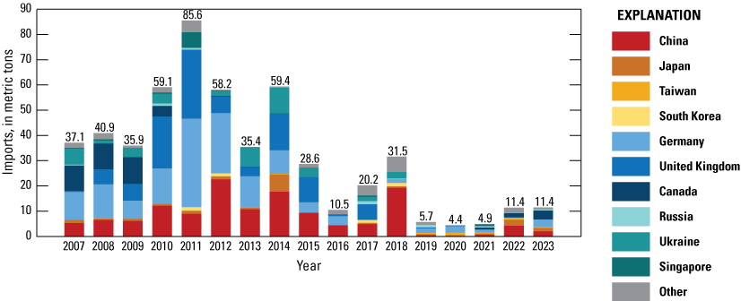
Graph showing U.S. imports of unwrought gallium metal (Harmonized Tariff Schedule of the United States code 8112.9210.00), by country, from 2007 to 2023, as reported by the United States. Data are from Zen Innovations AG (2024).
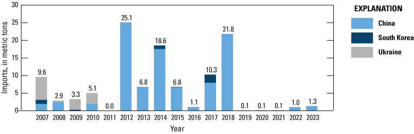
Graph showing U.S. imports of wrought gallium metal, as reported by trade partner, from 2007 to 2023. Data are from Zen Innovations AG (2024).
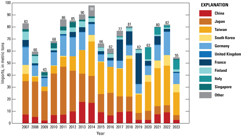
Graph showing U.S. imports of gallium-arsenide (GaAs) wafers doped (Harmonized Tariff Schedule of the United States [HTS] code 3818.0000.10) and undoped (HTS code 2853.9090.10), by country, from 2007 to 2023. Quantities are converted to gallium content assuming a content of 48.2 percent. Low-value imports (less than $200 per kilogram) were excluded. Data are collected at the district level. Data are from Zen Innovations AG (2024).
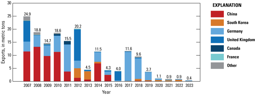
Graph showing U.S. exports of unwrought gallium metal, as reported by trade partners what other countries noted they exported to the United States (also known as mirror trade), from 2007 to 2023. Data are from Zen Innovations AG (2024).
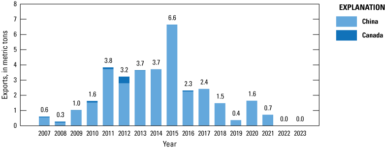
Graph showing U.S. exports of wrought gallium metal, as reported by trade partners what other countries noted they exported to the United States (also known as mirror trade), from 2007 to 2023. Data are from Zen Innovations AG (2024).
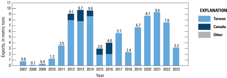
Graph showing U.S. exports of gallium-arsenide (GaAs) wafers doped, as reported by trade partners what other countries noted they exported to the United States (also known as mirror trade), from 2007 to 2023. Quantities are converted to gallium content assuming a content of 48.2 percent. Low-value imports (less than $200 per kilogram) were excluded. Data are from Zen Innovations AG (2024).
U.S. Gallium Consumption
Consumption of gallium metal and compounds was reported by the USGS based on survey responses and estimates (fig. 1.17; Jaskula, 2021). The decrease in U.S. consumption of gallium metal and compounds in the mid-2010s reflects the shift in manufacturing to Asia.
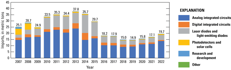
Graph showing U.S. consumption of gallium metal and compounds, by application, from 2007 to 2022, as reported in Jaskula (2021) and U.S. Geological Survey (2024).
Gallium metal and compounds were predominately used in the United States in integrated circuits (analog and digital) and optoelectronic devices (laser diodes, light emitting diodes [LEDs], photodetectors, and solar cells; fig. 1.17). The use of GaAs in analog integrated circuits includes radio frequency (RF) power amplifiers and switches, which are used in mobile handsets; wireless local-area network (WLAN) applications such as consumer electronics (for example, routers, game counsels, laptops, tables, and printers); and RF power applications for telecommunication infrastructure, and defense applications (for example, radar, electronic warfare and improvised explosive devices jammers, electronic countermeasures, and military communication; Yole Développement, 2018). Gallium nitride (GaN) is used in RF applications for telecommunication infrastructure; handset applications; defense applications (military radar, electronic warfare, and military communication); civilian radar and avionics; wired broadband; satellite communications; and RF energy applications (for example, plasma lighting, solid-state cooking, industrial drying and heating, medical tumor ablation, plasma scalpels, and automotive ignition; Yole Développement, 2019). GaN is also used in power applications for faster charging of consumer electronics; wireless charging; traction inverter, onboard chargers, and direct-current (DC)-to-DC converters in electric and hybrid electric vehicles; as well as in various power devices for data centers and industrial applications.
In photonics, gallium is used in edge emitting lasers, surface emitting lasers, vertical-cavity surface-emitting lasers that are found in smartphones (for three-dimensional imaging and sensing, autofocus, and proximity sensors), data centers, medical applications, machine vision systems, industrial heating systems, legacy consumer electronics (for example, laser compact disc, digital video disc, and optical computer mice), and light detection and ranging (lidar) for automotive applications (Yole Développement, 2018). Gallium is also used in LEDs across the spectrum, from ultraviolet (used in curing and disinfection), to red, orange, and yellow LEDs used in lighting and displays in consumer electronics, automotive lighting, horticultural lighting, and residential and decorative lighting, to infrared LEDs used in optical telecommunications, optical mice, and remote controls (Yole Développement, 2018). Gallium is also used in solar photovoltaic (PV) technologies, including copper-indium-gallium-diselenide (CIGS) thin-film solar cells as well as III–V high-efficiency solar cells. More recently, gallium is used as a dopant in p-type silicon PV (as an alternative to boron) to reduce light-induced degradation (Feldman and others, 2024). In China, gallium is also used as an additive in rare earth (neodymium-iron-boron [NdFeB]) permanent magnets (Løvik and others, 2015).
The quantity of net imports of gallium metal (11.5 t in 2022) was less than the quantity of reported consumption (19.7 t in 2022; table 1.9), suggesting that the trade data were indeed an underestimate. Unlike the net imports of the metals, net imports of GaAs wafers would likely be in addition to the U.S. consumption reported here. The total U.S. consumption was estimated from the reported metal and compound consumption and the net imports of GaAs wafers (table 1.19). To estimate the monetary value of the reported consumption of gallium metals and compounds, the import unit value for 2022, the weighted average of which was $404 per kilogram, was used.
Gallium in Semiconductor Applications
All U.S. consumption of gallium was in the semiconductor and related device manufacturing industry (Bureau of Economic Analysis [BEA] industry code 334413; Bureau of Economic Analysis, 2023). The value of shipments of that industry totaled $58.7 billion in 2021 (U.S. Census Bureau, 2022), which was equivalent to 10.6 percent of the $555.9 billion global semiconductor device industry for the year (World Semiconductor Trade Statistics GmbH, 2022).
Gallium is used in various compound semiconductors (such as GaAs, GaN, and gallium phosphide), which together along with other compound semiconductors (for example, indium phosphide, silicon carbide, and silicon germanium [SiGe]) represent a relatively small percentage of total semiconductor device market. The composition of the U.S. semiconductor and related device manufacturing industry’s (BEA industry 334314) revenues (fig. 1.18) provides some insights as to the percentage that may be linked to gallium. At a minimum, gallium was used in the production of all LEDs, which accounted for about 5 percent of the industry’s output in 2021. Gallium was also used in, at least in part, of several other product categories (for example, light sensitive and light-emitting devices, transistors, PV modules, diodes, and rectifiers).
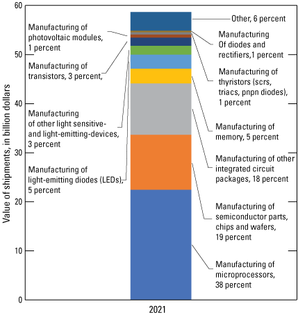
Graph showing value of shipments by the U.S. semiconductor and related device manufacturing (Bureau of Economic Analysis [BEA] industry 334413), in 2021, by product category. Data from previous years were used to estimate data that were withheld by the U.S. Census Bureau for 2021 (U.S. Census Bureau, 2022). %, percent.
Market research data were examined next. In 2021, revenues from the sales of compound semiconductor devices in the United States were estimated to be $4.6 billion (Mordor Intelligence, 2022). Globally, gallium-based compound semiconductors were reported to have generated at least $13.7 billion in 2021 out of a total of $22.9 billion for all compound semiconductors, or at least 59.7 percent (Mordor Intelligence, 2022). Assuming that this share is applicable to the United States, at least $2.8 billion of revenue was estimated to be from gallium-based semiconductor devices in 2021. This represented 4.7 percent of total U.S. semiconductor and related device manufacturing (BEA industry 334413) industry’s revenues for that year, similar to the lower bound identified when examining the composition of the industry’s output. Note that this was a rough estimate because market reports on the compound semiconductor market vary notably with no real consensus among them. For example, other market research reports (Market Research Future, 2023; MarketsandMarkets Research Pvt. Ltd., 2023a; Maximize Market Research Pvt. Ltd., 2023; Polaris Market Research, 2023; Precedence Research Pvt. Ltd., 2023; Verified Market Research, 2023) suggest that the global semiconductor device market size ranged from $34 billion to $43 billion in recent [2021–23] years. Taking the lower and upper values in that range and assuming the same ratio of U.S.-to-global compound semiconductors and gallium-based to other compound semiconductors, the value of U.S. gallium-based compound semiconductor devices likely was estimated to range from 4 billion to 5.2 billion, or about 7 to 9 percent of the total output of the industry. A value of 7 percent ±2 percent was selected for this analysis.
Gallium Sensitivity Analysis
Given the large uncertainties, a sensitivity analysis was performed where each of the key parameters in the assessment was varied from the baseline case to provide “low-impact” and “high-impact” cases (table 1.10).
Table 1.10.
Parameters used for a gallium sensitivity analysis.[GaAs, gallium arsenide]
Estimating New Equilibrium Quantities and Prices of Gallium, by Scenario
Based on the estimated price elasticities, production, product capacities, trade, and inventories, the new equilibrium quantities and prices for different levels of disruptions to China’s net exports of gallium (in all forms) to the rest of the world were estimated (tables 1.11–1.13). In these scenarios, imports and exports for all forms of gallium were assumed to decrease proportionally (figs. 1.19–1.21).
Table 1.11.
Estimated gallium quantities and prices based on different levels of restriction of China’s net exports of gallium for the baseline case.Table 1.12.
Estimated gallium quantities and prices based on different levels of restriction of China’s net exports of gallium for the low-impact case.Table 1.13.
Estimated gallium quantities and prices based on different levels of restriction of China’s net exports of gallium for the high-impact case.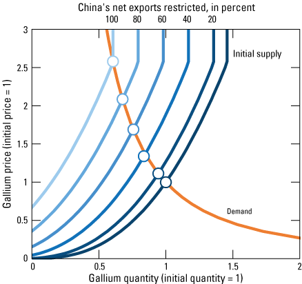
Graph showing gallium demand and supply curves for the rest of the world at different levels of restriction of China’s net exports of gallium for the baseline case.
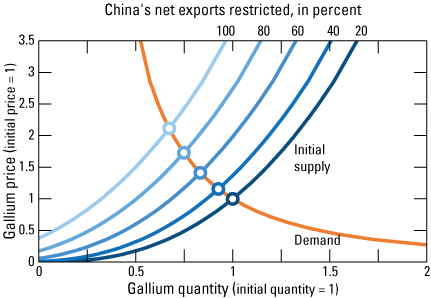
Graph showing gallium demand and supply curves for the rest of the world at different levels of restriction of China’s net exports of gallium for the low-impact case.
Graph showing gallium demand and supply curves for the rest of the world at different levels of restriction of China’s net exports of gallium for the high-impact case.
Germanium
World Germanium Production and Production Capacity
There is a high degree of uncertainty regarding world germanium production. Estimates of germanium world primary production in 2022 were prepared based on the best available information (table 1.14).
Table 1.14.
Estimated world production of primary germanium by country, in 2022.| Country | Primary production, in metric tons | Primary production capacity, in metric tons | References and notes |
|---|---|---|---|
| Belgium | 4 | 10 | Quantities were estimated based on information provided by (Grohol and Veeh, 2023) and exclude secondary production. |
| Canada | 20 | 30 | Production quantity estimated based on reported exports under HS codes 28.2560.00 and 28.2739.00, with unit values above $300 per kilogram. Capacity was estimated based on recent historic production levels. |
| China | 180 | 309 | Quantities are reported product estimates of germanium metal (Antaike, 2023; Asian Metals Ltd., 2023b) |
| Finland | 0 | 20 | There has been no primary germanium production in Finland since 2016 (Lauri, 2019; Grohol and Veeh, 2023). Production capacity was estimated based on previously reported production (Geological Survey of Finland, 2016). |
| Russia | 6 | 20 | Estimates were based on information for 2023 from news reports (Stolyarov and others, 2023). |
| Ukraine | 0 | ≤1 | Estimates suggest production may have been around 1 metric ton (Reichl and Schatz, 2023), but it is believed that production was likely less than 1 metric ton or 0. |
| Total | 210 | 389 | |
| Total outside China | 30 | 80 |
Note that China’s primary germanium metal production has reportedly grown from 102.9 t in 2019 to 156 in 2021 and 180 t (or possibly 187.5 t) in 2022 (Antaike, 2023; Asian Metals Ltd., 2021, 2023b). China’s production capacity has also reportedly increased notably from 230 t in 2019 to 307 t in 2021 and 309 t in 2022, with nearly half of the production capacity coming from 5 operations in Yunnan province out of a total of 10 operations in the country (Asian Metals Ltd., 2023b). In contrast, production in Finland stopped in 2015–16 (Lauri, 2019; Grohol and Veeh, 2023).
In addition to the production noted in the table above, Japan (Japan Organization for Metals and Energy Security, 2023), Belgium (Umicore, 2021), Germany (Grohol and Veeh, 2023), and the United States (U.S. Geological Survey, 2024) produced germanium from imported and secondary (new or preconsumer scrap) sources. These quantities are excluded from table 1.14 above to avoid double-counting.
China’s Trade of Germanium Products
China’s Ministry of Commerce announced on July 3, 2023, the export controls on six germanium products (table 1.15; Ministry of Commerce and General Administration of Customs (China), 2023).
Table 1.15.
Harmonized System codes for germanium products with recent export controls by China.[Harmonized Commodity Description and Coding System (HS) codes are from Ministry of Commerce and General Administration of Customs [China] (2023)]
Trade data were only available at the 8-digit HS codes (figs. 1.22–1.27; table 1.16). Therefore, trade data of germanium under most of these codes were obscured because they include other products that do not contain germanium. Specifically, only trade data for germanium metal (under HS codes 8112.9210 and 8112.9910; fig. 1.22 and 1.25) are directly discernable as containing germanium in the data reported by China. However, trade of germanium oxides (fig. 1.23 and 1.26) and chlorides (fig. 1.24 and 1.27) can be estimated based on excluding materials below a threshold unit value, which was set at $300 per kilogram. Additionally, Taiwan reports trade of germanium wafers but the reported trade with China is negligible and is ignored to avoid double counting.
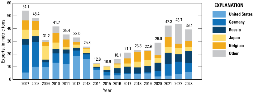
Graph showing China’s exports of germanium metal (Harmonized System codes 8112.9210 and 8112.9910), as reported by China, by country, from 2007 to 2023. Data exclude low-value (less than $300 per kilogram) shipments that were thought to be low-purity scrap. Data are from Zen Innovations AG (2024).
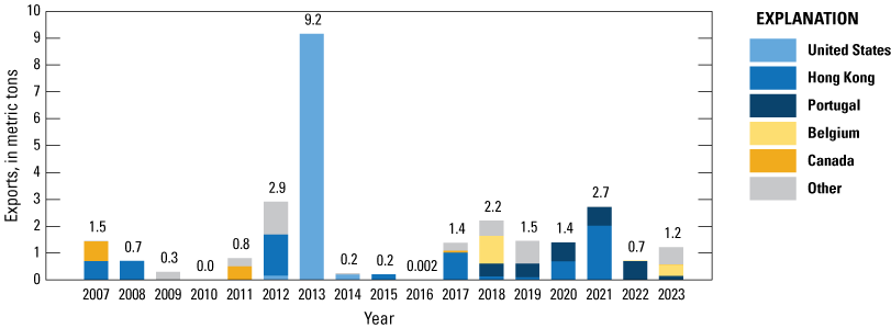
Graph showing China’s exports of germanium oxides (Harmonized System code 2825.6000), as reported by China, by country, from 2007 to 2023. Data exclude low-value (less than $300 per kilogram) shipments that were thought to be zirconium oxide. Data are from Zen Innovations AG (2024).
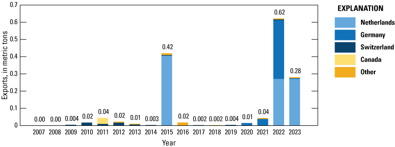
Graph showing China’s exports of germanium chlorides (Harmonized System code 2827.3990), as reported by China, by country, from 2007 to 2023. Data exclude low-value (less than $300 per kilogram) shipments that were thought to be other chlorides. Data are from Zen Innovations AG (2024).
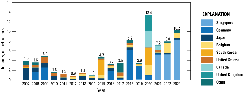
Graph showing China’s imports of germanium metal (Harmonized System codes 8112.9210 and 8112.9910), as reported by China, by country, from 2007 to 2023. Data exclude low-value (less than $300 per kilogram) shipments that were thought to be low-purity scrap. Data are from Zen Innovations AG (2024).
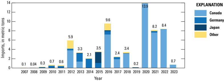
Graph showing China’s imports of germanium oxides (Harmonized System code 2825.6000), as reported by China, by country, from 2007 to 2023. Data exclude low-value (less than $300 per kilogram) shipments that were thought to be zirconium oxide. Data are from Zen Innovations AG (2024).
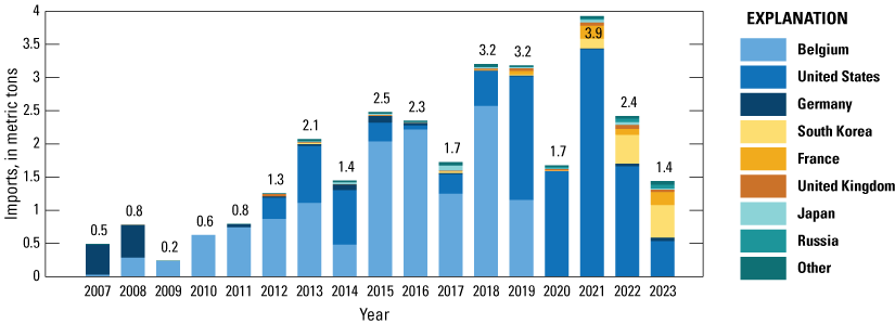
Graph showing China’s imports of germanium chlorides (Harmonized System code 2827.3990), as reported by China, by country, from 2007 to 2023. Data exclude low-value (less than $300 per kilogram) shipments that were thought to be other chlorides. Data are from Zen Innovations AG (2024).
Given the uncertainty in the trade data, China’s total net exports were estimated by using reported production, consumption, and market surplus data. Specifically, China’s net exports were estimated to likely be about 35 t in 2022 given reported domestic production (180 t of germanium), consumption (122 t of germanium) and market surplus (23 t of germanium; table 1.17; Antaike, 2023). This suggested that the 35 t of estimated trade data may be missing roughly 9 t of China’s net exports of germanium.
Table 1.17.
China’s reported production, consumption, market surplus, and net exports.| Category | Quantity, in metric tons of germanium | References and notes |
|---|---|---|
| Primary production | 180 | Antaike (2023) |
| Domestic consumption | 122 | Antaike (2023) |
| Market surplus (net additions to inventories) | 23 | Antaike (2023) |
| Total net exports based on mass balance | 35 | Primary production less consumption and market surplus |
| Estimated net exports from trade data | 26 | See table 1.16 |
| Missing net exports from trade data estimate | 9 | Total exports less reported net exports |
Germanium Inventories Outside of China
Aside from China, there were some germanium inventories held by governmental agencies. In the United States, the Defense Logistics Agency held 14 t of uncommitted germanium metal as of 2022 (Thomas, 2023). Japan listed germanium as a critical mineral for stockpiling and was thus assumed to have 180 days of inventories (International Energy Agency, 2023a). In 2022, Japan imported 3.709 t of unwrought germanium metal (Japan HS code 8112.9291.0) and 13.221 t of germanium oxide (GeO2; 9.178 t of germanium content; Japan HS code 2825.6010.0; Zen Innovations AG, 2024). Japanese exports were very small at 93 kilograms (kg) of GeO2 (64.5 kg of germanium content; Zen Innovations AG, 2024). Japan’s imports of GeO2 were reported separately from any other commodity, but their exports are reported with zirconium oxide (ZrO2), and thus the standard unit value cutoff ($300 per kilogram) was applied. Japan’s net imports were thus estimated to be 12.8 t of germanium. Assuming net imports were equal to consumption, Japan was estimated to be holding 6.3 t of germanium in inventories.
Even though South Korea has a list of critical mineral commodities that were to be held in strategic inventories, germanium was not listed among them (International Energy Agency, 2023b). The scenarios used in this report assumed no inventories of germanium were held by South Korea. No information was found for any other inventories. Total germanium inventories for the rest of the world thus summed to 20.3 t of germanium.
U.S. Germanium Trade
The United States imported germanium under several HTS codes. Specifically, U.S. imports and exports include GeO2 and ZrO2 (HTS code 2825.60.0000); unwrought germanium (HTS code 8112.92.6000 starting in 2007, HTS code 8112.30.6000 before 2007); germanium powder (HTS code 8112.92.6500 starting in 2007); articles of germanium wrought, waste scrap, powders not elsewhere specified or included (HTS code 8112.99.1000 starting in 2007); and germanium waste and scrap (HTS code 8112.30.3000 before 2007; figs. 1.28–1.32; tables 1.18–1.22). To estimate the germanium content, low-value (less than $300 per kilogram) entries are excluded because it was believed they were ZrO2 of the oxide HTS code or low-quality scrap for the metal HTS or misclassified materials. The resultant quantities for the oxide HTS code were further multiplied by 69.4 percent to obtain germanium content by using standard stoichiometric ratios (Commission on Isotopic Abundances and Atomic Weights and International Union of Pure and Applied Chemistry, 2021).
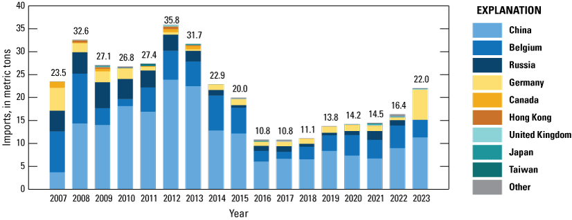
Graph showing U.S. imports of germanium metal (Harmonized Tariff Schedule of the United States codes 8112.92.6000, 8112.92.6500, 8112.99.1000), in metric tons of germanium content, by country, from 2007 to 2023. Data exclude low-value (less than $300 per kilogram) shipments that were thought to be low-purity scrap.
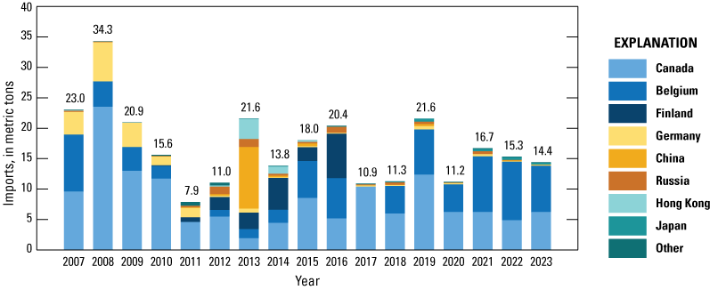
Graph showing U.S. imports of germanium oxide (Harmonized Tariff Schedule of the United States code 2825.60.0000), in metric tons of germanium content, by country, from 2007 to 2023. Data exclude low-value (less than $300 per kilogram) shipments that were thought to be zirconium oxide.
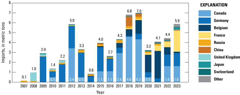
Graph showing U.S. imports of germanium chlorides (Harmonized Tariff Schedule of the United States codes 2827.39.9000), in metric tons of germanium content, by country, from 2007 to 2023. Data exclude low-value (less than $300 per kilogram) shipments that were thought to be other chlorides. Imports from Canada are enumerated to highlight that they match data from a different data source.
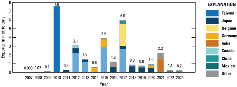
Graph showing U.S. exports of germanium oxide (Harmonized Tariff Schedule of the United States code 2825.60.0000), in metric tons of germanium content, from 2007 to 2023. Data exclude low-value (less than $300 per kilogram) shipments that were thought to be zirconium oxide.
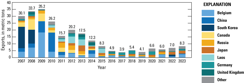
Graph showing U.S. exports of germanium metal (Harmonized Tariff Schedule of the United States codes 81.1292.6100 and 81.1299.100), in metric tons of germanium content, from 2007 to 2023. Data exclude low-value (less than $300 per kilogram) shipments that were thought to be low-purity scrap.
Table 1.18.
Summary of quantities of U.S. imports of germanium, by type.[Values are in metric tons of germanium content. HTS, Harmonized Tariff Schedule of the United States (U.S. International Trade Commission, 2024)]
Table 1.19.
Summary of value of U.S. imports of germanium by type.[Values are in million U.S. dollars. HTS, Harmonized Tariff Schedule of the United States (U.S. International Trade Commission, 2024)]
Table 1.20.
Summary of quantities of U.S. exports of germanium by type.[Values are in metric tons of germanium content. HTS, Harmonized Tariff Schedule of the United States (U.S. International Trade Commission, 2024)]
Table 1.21.
Summary of value of U.S. exports of germanium by type.[Values are in million U.S. dollars. HTS, Harmonized Tariff Schedule of the United States (U.S. International Trade Commission, 2024)]
Table 1.22.
Summary of U.S imports, exports, and net import of germanium quantity, value, and unit value.Finally, trade of germanium tetrachloride (GeCl4) were reported under HTS code 2827.39.9000 (other chlorides not elsewhere specified or included; tables 1.18–1.19). Low-value (less than $300 per kilogram) trades were excluded under the assumption that low-value materials were other (nongermanium) chlorides. The results were then multiplied by 33.9 percent to obtain germanium content by using standard stochiometric ratios (Commission on Isotopic Abundances and Atomic Weights and International Union of Pure and Applied Chemistry, 2021). Although there is uncertainty in this approach, GeCl4 imports from Canada to Seattle, Washington, for 2016–19 match perfectly with those reported to Teck America, Inc. in the U.S. Environmental Protection Agency (2020, 2023)136 Chemical Data Reporting (CDR) database under GeCl4 (table 1.18), which would indicate the accuracy of the approach used in this report. Moreover, this cutoff value was varied in the sensitivity analysis. In addition to germanium metal, oxides, and chlorides, germane gas (GeH4) was likely imported by the United States under HTS code 2804.29.0050, where it was combined with other rare gases, making the trade of GeH4 undiscernible. Using bill of lading data, a total of 268 canisters were identified as being imported into the United States in 2022 (ImportGenius, 2024). Assuming each canister contained 2.6 kg of GeH4 (Air Liquide Advanced Materials, 2015), total imports of germanium contained in these canisters were calculated to be approximately 0.66 t. No exports of GeH4 were reported. Trade of germanium wafer is reported under HTS code 3819.00.0090, but that code also contained various types of wafers (aside from GaAs wafers), so the quantity of germanium wafers cannot be discerned. However, Taiwan reports germanium wafer trade separately under HS code 3818.00.10200, but no trade was reported with the United States in 2022. Overall net imports for the United States were estimated to be 29.5 t in 2022.
U.S. Germanium Consumption
The USGS estimated U.S. consumption of germanium to be roughly 30 metric tons per year (t/yr) for the past few years (U.S. Geological Survey, 2024). This estimate matches the quantities reported (table 1.23) by the U.S. Environmental Protection Agency (EPA) in the Chemical Data Reporting (CDR) database (U.S. Environmental Protection Agency, 2023). Note, however, that the quantity reported in the CDR includes manufacturing of GeCl4, which is noted in the CDR database as recycled materials. This is presumed to be entirely new (preconsumer) scrap recycling from fiber optic manufacturing and thus would not be counted in a consumption calculation. Also, note that the CDR data do not include imports of germanium metal or GeH4. Finally, note that there are certain annual reporting thresholds (U.S. Environmental Protection Agency, 2020) for the CDR so the absolute quantities reported in the CDR are likely an undercount. The quantity consumed in the United States was estimated based on a calculated apparent consumption, which is the sum of domestic production, net imports, and any stock changes.
Table 1.23.
Reported U.S. consumption of germanium compounds in kilograms of contained germanium.[By year, company, and form, as reported in the Chemical Data Reporting database (U.S. Environmental Protection Agency, 2023). Quantities are converted to germanium content based on standard stoichiometric ratios. Percentages may not add to totals shown due to rounding. GeCl4, germanium tetrachloride; GeO2, germanium oxide]
The Red Dog zinc-lead mine in Alaska produces a zinc concentrate that contains germanium (U.S. Geological Survey, 2024). A portion of this concentrate is sent to a zinc-lead refinery in Canada where germanium is recovered as a byproduct in the form of GeO2 and GeCl4. However, given that germanium recovery takes place outside of the United States, it is not included in the U.S. production estimate.
The Defense Logistics Agency initiated a germanium recycling program in 2022 to recycle germanium lenses from decommissioned military equipment but it was not clear what, if any, quantities were recovered in 2022 (Reece, 2022). Production in the United States, thus, was likely limited to secondary (new scrap recycled) production. Specifically, a refinery in Oklahoma recovered germanium from industry scrap to produce GeCl4 for fiber optics (likely to be the quantities listed in table 1.23 as being manufactured; U.S. Geological Survey, 2024). Germanium wafers were produced by a company in Utah from imported and recycled germanium (U.S. Geological Survey, 2024). Additionally, a zinc smelter in Tennessee, which produces germanium leach concentrates, was planning to construct a gallium and germanium processing plant that would have the capability of recovering 40 t/yr of germanium (U.S. Geological Survey, 2024). Given that there was no primary germanium production, no old (postconsumer) scrap recycling in the United States, and no reported releases from inventories (U.S. Geological Survey, 2024), U.S. apparent consumption of primary germanium is equivalent to net imports, which for 2022 was estimated to be 29.5 t.
Germanium Applications
Data from the USGS Mineral Commodity Summaries (U.S. Geological Survey, 2024) suggest that, in recent years, germanium was used in the following proportions in the United States: 40 percent in fiber optics, 30 percent in infrared optics, 20 percent in electronics and solar applications, and 10 percent in other uses. These quantities were last reported for 2016 and continue a shift during the past few decades towards larger quantities of germanium being used in fiberoptics (Butterman and Carlin, 2004).
Data from Asian Metals suggest that global uses of germanium in 2020–22 were as follows: 30 percent in optical fiber, 20 percent in infrared, 20 percent as polymerization catalyst, 15 percent in solar PV, and 15 percent in other uses (Asian Metals Ltd., 2023b).
Germanium in Fiberoptic Systems
GeCl4 is oxidized to form GeO2, which is then used as a dopant in fiber optics to slightly increase the refractive index of the core glass relative to the cladding. The U.S. market for fiberoptic preform (the solid glass rod precursor to optical fibers and, ultimately, optical fiber cable that is manufactured using GeCl4 and SiCl4) was estimated to be $412 million, or roughly 10 percent of the global market in 2021 (Grand View Research, 2023). Similarly, the North American market demand for optical fiber cable was estimated to have been 64 million fiber-kilometers (13 percent of world demand) in 2018 (Sterlite Technologies Ltd., 2023) and to have increased to 82 million fiber-kilometers (16 percent of world demand) in 2021 Sterlite Technologies Ltd., 2023). This represents a major increase compared with the past few decades. In 1986, for example, U.S. production capacity for optical fiber cable was estimated to be a little more than 3 million fiber-kilometers (Johnson and Linkins, 1988). Factoring in net exports (under HTS codes 8544.70.0000 and 9001.10.0030) to estimate production (rather than demand) and the U.S. share of North American production (estimated to be about 56 percent for 2022; Gaurav, 2018), U.S. manufacturing of optical fiber cable was estimated to be 48 million fiber-kilometers or 9.7 percent of the world total (roughly the same percentage of the world total for the preform market).
The quantity of germanium used in optical fiber cable was estimated based on the length of optical fiber cable manufactured and the germanium content per unit of optical fiber cable length. Single-mode cables typically have a core with diameters that range between 8.3 to 10 micrometers (μm), whereas multimode cables typically have a core with diameters that range from 50 to 100 μm, with the most common size in the United States being 62.5 μm (Gaurav, 2018). In North America, roughly 35 percent of the market is for single-mode cables, and 54 percent is for multimode cables, with the remaining 10 percent being plastic optical fiber (Grand View Research, 2019). Using these market fractions and diameters, an assumed GeO2 content of 4 percent (2.8 percent germanium; Bell Labs-Lucent Technologies, 1997), and a density of 2.2 grams per cubic centimeter (g/cm3) for fused silica, the quantity of germanium contained in optical fiber cable produced in the United States in 2021 was estimated to be approximately 5 t (table 1.24).
Table 1.24.
Germanium contained in fiberoptic cable laid in the United States in 2021–22.There are, however, significant losses of germanium during oxidation (70 to 85 percent of the starting GeCl4 is not oxidized) and deposition (50 percent efficiency), leaving only 8 to 15 percent of the starting germanium ultimately being incorporated into the final optical fiber cable (Licht and others, 2015). Around 80 to 95 percent of the germanium that enters these waste streams is regularly recovered (Licht and others, 2015). As such, 60 percent of the germanium that is used in the production of optical fiber cable comes from recycled materials (Jorgenson, 2006; Licht and others, 2015). The ratio of germanium from primary materials to germanium incorporated in the optical fiber cable was, in turn, calculated to be 2.68:1 (Licht and others, 2015). Accordingly, the total quantity of primary germanium used in the manufacture of fiber optics in the United States was estimated to be roughly 13.3 t (4.97 t×2.68). This is similar to the quantity estimated to have been consumed during the past few decades (Butterman and Jorgenson, 2005).
According to the North American Product Classification System (NAPCS), in the United States, manufacturing of fiber optic cable for communication and for all other applications is classified under two NAPCS collection codes, respectively: 2039.15.000 and 2039.17.5000. These two commodities are produced mainly by the fiberoptic cable manufacturing industry (North America Industry Classification System [NAICS] code 335921). To a much smaller degree, they are also produced under the other communication and energy wire manufacturing (BEA industry 335929) industry. In the BEA input-output tables (Bureau of Economic Analysis, 2023), these two NAICS codes are combined under the communication and energy wire and cable manufacturing (code 335920) industry group. The value of the commodities produced under these two NAICS codes totaled $3,132 million in 2021, about 23 percent of the 335920 industry group’s output (table 1.25).
Table 1.25.
U.S. applications for germanium and connections to industry codes.[BEA, Bureau of Economic Analysis; NAICS, North American Industry Classification System; NAPCS, North American Product Classification System; τ, percentage of BEA industry output that uses the mineral commodity listed, also known as percent connected; NA, not applicable; %, percent (expresses fraction of U.S. consumption of germanium consumed by the application or subcategory; values may not add to totals shown due to rounding]
NAICS/NAPC code data from 2021 Annual Survey of Manufacturers (U.S. Census Bureau, 2022).
NAPCS code data from 2017 Economic Census (U.S. Census Bureau, 2017a) multiplied by a 50% market share for germanium lenses.
Market research reports (Szwedo, 2002; Maximize Market Research Pvt. Ltd., 2023; Global Industry Analysts Inc., 2024).
Market research reports (Grand View Research, 2014; 360 Research Reports, 2022).
Market research reports (Future Markets Insights, 2016; Grand View Research, 2022).
The NAPCS code 2039.15.000 was also produced by several other NAICS codes, namely 327212 ($52.8 million), 327215 ($5.4 million), 33441 ($11.9 million), and 339999 ($125.8 million). The value of this NAPCS code as a percentage of the corresponding BEA industry group was relatively small, ranging from 0.01 percent to 0.44 percent. The germanium quantity for this application was thus allocated proportionally to the value of shipments of each corresponding BEA industry group.
Germanium in Infrared Optics
Given its transparency to part of the infrared electromagnetic spectrum, germanium is used as lenses and windows for infrared optical systems in defense and nondefense applications, including surveillance, reconnaissance, and target-acquisition applications (Shanks and others, 2017). Germanium competes with other materials (for example, zinc selenide) and is optimal for night vision and thermal imaging in the medium- and long-wave infrared band, ideally between 8 and 12 μm (Rowe, 2024). U.S. consumption of infrared lenses was estimated to represent less than one-third (32.5 percent) of the global market in 2017 (QY Research, 2019). Assuming this proportion holds for germanium lens production, U.S. consumption of germanium in infrared lenses was estimated to be as follows: global germanium use in infrared optics was about 30 t (152 t for China’s plus the rest of the world’s consumption of primary germanium × 20 percent market share for the infrared lens application), of which the United States consumed about 9.9 t (30 t × 32.5 percent market share for the United States).
Data for defense and nondefense sales of imaging and sensors, by product, were estimated for 2001–05 by the Office of Strategic Industries and Economic Security at the U.S. Department of Commerce Bureau of Industry and Security (fig. 1.33; DeMarines and Botwin, 2006). For 2005, total U.S. defense (about 70 percent) and nondefense (about 30 percent) sales were less than $3.9 billion across all imaging and sensor products, with cooled infrared (thermal) imaging system devices and components representing the largest category at less than $1.2 billion in 2005. Night vision goggles were estimated to be $270 million in 2005. This is the only category of imaging and sensor device that has a directly identifiable NAPCS collection code (2018.57.5012: Manufacturing of night vision goggles and equipment) for which sales in 2017 in the United States were reportedly $210 million (U.S. Census Bureau, 2017a)—a sales value that is similar to the levels of 2005. The remaining applications likely fall under the manufacturing of light reconnaissance and surveillance electronic systems and equipment (NAPCS collection code 2017.50.0003) and search, detection, navigation, guidance, aeronautical, and nautical system and instrument manufacturing (NAICS code 334511). In 2017, this NAPCS code, which includes bomber-defense equipment, fire control equipment, infrared fuses, space satellite, and other infrared detection and warning systems, sniper scopes, snooperscopes, night-driving equipment, mapping equipment, photographic equipment, and wake detection generated $7.1 billion in sales.
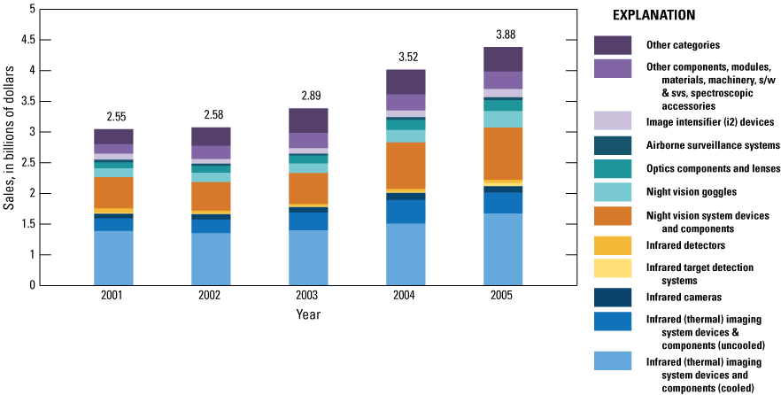
Graph showing U.S. manufacturers sales on defense and nondefense sales of imaging and sensors, by product, from 2001 to 2005, as reported by the Office of Strategic Industries and Economic Security at the U.S. Department of Commerce Bureau of Industry and Security (DeMarines and Botwin, 2006).
Globally, there was a significant increase in demand in 2020 for thermal imaging and sensing (cameras and detectors) from $5 billion in 2019 to $7.6 billion due to the need for fever detection during the COVID–19 pandemic. However, in 2021, demand decreased to $6.7 billion and returned to traditional infrared applications (Clouet, 2023). Demand decreased further in 2022 to about $6.3 billion due to a chip shortage caused from supply chain shortages (Clouet, 2023). Another market research report suggests that the North American imaging market was valued at about $3 billion out of the $6.4 billion global market in 2022, or roughly 47 percent (MarketsandMarkets Research Pvt. Ltd., 2023b). Again, this value for 2022 is similar in magnitude to that value reported in 2005 in the report by the Office of Strategic Industries and Economic Security (DeMarines and Botwin, 2006). It is also similar to sales revenues for 2009, which were estimated to be $6.6 billion globally for military (88 percent) and commercial (12 percent) applications (Guberman, 2013).
As noted earlier, germanium competes with other materials in this application. Germanium crystals were estimated to have been used in approximately 60 percent of lower and midrange infrared-optical systems, and about half of all high-end devices used lenses used germanium crystals (Guberman, 2011). Other market data suggest that infrared cameras using germanium lenses comprise roughly 40 percent of the market, with silicon, zinc selenide, and sapphire comprising the remaining 60 percent (Grand View Research, 2015).
Taking all this information into account, the use of germanium in infrared optics was split between BEA industry groups optical instrument and lens manufacturing (333314) and search, detection, and navigation instruments manufacturing (334511). Within BEA code 333314, manufacturing of night vision goggles and equipment (NAPCS code 2018.57.5012) was assumed to be the only applicable code. Its sales were $210 million or 4.8 percent of the 333314 industry (U.S. Census Bureau, 2017b). Germanium lenses were assumed to represent 50 percent of the market for night vision goggles. This percentage varied in the sensitivity analysis to 40 percent and 60 percent in the low- and high-impact cases, respectively.
Within BEA code 334511, manufacturing of light reconnaissance and surveillance electronic systems and equipment (NAPCS 2017.50.0003) was assumed to be the only applicable code. It generated $7.1 billion in sales in 2017 or 13.8 percent of the industry’s output that year. Of this NAPCS code, 50 percent (±10 percent in the sensitivity analysis) was assumed to use germanium lenses per market data, (Grand View Research, 2015; Guberman, 2011) equaling about $2.86 billion in sales. These sales combined with the $210 million in sales of night vision goggles yield a total of $3.1 billion, which matches the market data reported previously. The use of the germanium material (9.8 t) was split between BEA codes 333314 and 334511 based on these sales values, as well, with 93 percent (9 t) for 334511 and 7 percent (0.8 t) for 333314.
Germanium in Semiconductor (Electronic and Solar PV) Applications
Germanium is used as a single element substrate and as a IV–IV (SiGe) compound semiconductor and epitaxial layer in high-efficiency solar PV predominately for space applications (for example, satellites) but also in concentrated solar PV for terrestrial applications, as well as in transistors (for example, SiGe heterojunction bipolar and silicon-on-insulator) and high-brightness LEDs. All these applications fall under the semiconductor and related device manufacturing (334413) industry.
Of the global compound semiconductor device market, an estimated 7 percent ($2.6 billion) was reportedly based on SiGe substrates (Maximize Market Research Pvt. Ltd., 2023). Market research estimates suggest that North America was the largest producing and consuming region for SiGe materials and devices, with a market share of about 35 percent for 2001–06 (Szwedo, 2002). Assuming this percentage holds, the total value of SiGe-based devices in North America would be roughly $0.9 billion, or 1.5 percent of the 334413 industry’s output. Another market research report estimated the global SiGe semiconductor material and device market to be $8.3 billion, with the U.S. market valued at $2.3 billion (Global Industry Analysts Inc., 2024). An estimated 47 to 60 percent of the material and device market is estimated to be the devices (Szwedo, 2002), suggesting that the U.S. SiGe device market accounts for about $1.1 billion to 1.4 billion (or 1.9 to 2.4 percent of the 334413 industry). The average value was selected for the baseline case, and the lower and upper values were used in the low-impact and high-impact cases of the sensitivity analysis.
Despite several advantages, triple junction III–V (GaAs) high-efficiency solar PV cells are only used in niche applications (namely, high concentration PV, space solar cells, and emerging defense and transportation solar PV applications) due to their higher cost compared with crystalline-silicon or cadmium-tellurium solar PV (Horowitz and others, 2018; Yole Développement, 2018). It was estimated that these high-efficiency solar cells made up less than 1 percent of the solar PV market, 90 percent of which used germanium substrates, and the other 10 percent used GaAs substrate (Yole Développement, 2018). Solar PV accounts for roughly 1 percent of revenues of the 334413 industry (fig. 1.28), but most of that revenue is from crystalline silicon and cadmium-telluride thin film solar cells, with the high-efficiency solar cells representing a very small fraction.
Currently, germanium substrate is believed to have been produced in the United States by one company at its facility in St. George, Utah. It was estimated that roughly 5 percent of U.S. germanium metal imports were likely used for germanium substrate growth. That would place the quantity at 0.8 t of germanium. A recent life cycle assessment estimates that it takes about 15.52 g of primary germanium to make a 6-inch germanium wafer (with a net of 14.2 g comprising the wafer and the rest being recycled or lost; Umicore, 2022). Thus, an estimated 52,000 6-inch equivalent germanium wafers were produced in the United States. Six-inch germanium wafers generally cost around $100 and represent 12.5 to 20 percent of the value of the solar cells (Wilson and others, 2020). At 52,000 6-inch wafer equivalent, the solar cells manufactured in the United States would thus be valued at $26 million to $42 million. This would equate to 0.04 to 0.07 percent of the 334413 industry’s output, which would be within the rounding error of this report’s assessment of the fraction of other germanium-based semiconductor devices.
Yole Développement (2018) suggests that 18,400 6-inch-equivalent GaAs substrate wafers were used in space solar applications (out of a total of 21,700 6-inch wafer equivalents for solar PV applications in general) and that there were roughly nine times more germanium substrate wafers than GaAs wafers for solar PV applications. This suggests that there were 166,000 germanium substrate 6-inch equivalent wafers used for space solar PV (195,000 6-inch-equivalent germanium wafers for solar PV applications), globally. With an estimated content of 14.2 g of germanium per wafer, it was estimated that 2.3 t of germanium was sent to space in 2022. This matches an estimate of 2 kg noted by Ohlmann and others (2023). It also suggests that the United States produced roughly 27 percent of the world’s germanium substrates.
GeH4, along with silane (SiH4), is the precursor gas used to form and deposit the epitaxial layer and amorphous SiGe on wafers. It can be used in solar cells, as well as implantation and doping for semiconductors and photonic applications. As noted previously, approximately 0.66 t of GeH4 was estimated to have been imported into the United States in 2022. GeH4 may have also been produced domestically from imported GeO2 and, to a lesser degree, GeCl4. A leading producer of germane, Voltaix (which was acquired by Air Liquide in 2016), had a stated production capacity to produce 20 t of GeH4 per year at its Branchburg, New Jersey, operation (Voltaix, 2010). There was at least one other company with the capability to produce, but the actual amount produced in 2022 was not known. However, it was estimated that the U.S. demand for germane was $56.84 million in 2021, representing a 39.35 percent share of the world market (QY Research, 2022). An assumed unit price of $2,200 per kilogram GeH4 yields an estimated quantity of 25.8 t of GeH4 (24.5 t of germanium content) demand in the United States. Only 15 percent of the GeH4 is deposited in the manufacturing process (Lee, 2010). Assuming that the material that was not deposited was recycled with high efficiency (about 95 percent), approximately 4.7 t of germanium from primary sources was estimated to have been used in the United States. Therefore, the total amount of primary germanium used in semiconductor and solar applications was estimated to be 5.6 t.
Germanium in Polymerization Catalysts for Polyethylene Terephthalate
Germanium is used as a polymerization catalyst to produce polyethylene terephthalate (PET). In 2022, North American PET production capacity represented 13.5 percent of the world’s production capacity (4.7 out of 34.8 million metric tons; Lamb, 2022). However, unlike manufacturers in Japan (Japan Organization for Metals and Energy Security, 2023), manufacturers in the United States did not use germanium as a catalyst for PET, opting to use the market dominant and less expensive antimony- (or perhaps titanium-) based catalysts instead (Guberman, 2016).
Germanium in Radiation Detectors
High-purity germanium crystals are used in solid-state radiation detection equipment for use in particle accelerators, identification of radioactive waste, nuclear power plants, the detection of illicit or clandestine nuclear material trafficking, medical diagnosis, weather, and space applications. This equipment is manufactured by the other measuring and controlling device manufacturing (NAICS industry 334519) under the manufacturing of nuclear radiation detection and monitoring instruments (NAPCS collection code 2017550000) industries. This NAICS industry falls under the watch, clock, and other measuring and controlling device manufacturing (BEA code 33451A) industry. In 2021, the values of sales of these BEA, NAICS, and NAPCS codes were $13.8 billion, $11.3 billion, and $1.1 billion, respectively.
The radiation detection, monitoring, and safety market is comprised of three types of detectors: gas-filled, solid-state, and scintillators (Grand View Research, 2014). Gas-filled detectors and scintillators do not use germanium. Solid-state detectors, which typically use either germanium or silicon (Mirion Technologies Inc., 2023), represent about 14 percent of the market (Grand View Research, 2014). A market research report suggests that the global semiconductor radiation detector market was valued at $360.5 million in 2022 (360 Research Reports, 2022). The United States and North America market share was estimated to be 43 percent (Grand View Research, 2014; 360 Research Reports, 2022). Germanium-based detectors reportedly represent 65 percent of the market (360 Research Reports, 2022). Based on these figures, germanium-based detector sales were estimated to be approximately $100 million or about 0.7 percent of the 33451A BEA industry group. This market share percentage was varied in the sensitivity analysis from 33 to 100 percent.
A startup U.S. company reported $5.5 million in sales in 2021 based on 55 germanium-based detector units at $100,000 per device (McCarthy, 2022). Assuming each of their devices has a 60 cubic centimeter (cm3) germanium segmented detector (PHDS Co., 2023), that would be the equivalent to 320 g of germanium per device. Taking the total sales for the United States (which is predominately from two companies: Mirion and Ametc Ortec) and a production efficiency of 80 percent, a total of 0.4 t of germanium was estimated to be used in radiation detection in 2021–22.
Germanium in Positron Emission Tomography
Bismuth germanium oxide (BGO, Bi4Ge3O12) is one of several types of detectors used in positron emission tomography scanners. The U.S. market for positron emission tomography scanners was estimated to be $489.8 million in 2021, roughly one-quarter of $1.94 billion global market (Grand View Research, 2022). BGO, one of several types of detectors, reportedly represented 29.5 percent of the global positron emission tomography market in 2015 (Future Markets Insights, 2016). Assuming this market share holds for the United States, the total market value of BGO in the United States would amount to approximately $145 million. This value represents 0.4 percent of the electromedical and electrotherapeutic apparatus manufacturing (NAICS code 334510) industry, which positron emission tomography scanner manufacturing falls under. The market share percentage varied from 10 to 50 percent in the sensitivity analysis.
The global market value of BGO crystals themselves was estimated to be $39 million in 2022 (Business Research Insights, 2024). Assuming the U.S. market share of 24 percent for PET scanners holds also for BGO crystals, a value of $9.4 million was obtained. Although BGO crystal prices can vary notably, an individual crystal is assumed to cost roughly $40 per cubic centimeter (Epic-Crystal, 2024). Based on this value [equating to a density of 7.13 g/cm3 (Luxium Solutions, 2022) or a germanium content of 17.49 percent (based on standard stoichiometry)], for each U.S. dollar, BGO crystal was estimated to contain 0.03 g of germanium. At $9.4 million of BGO crystals, the amount of germanium used in the United States would be roughly equivalent to 0.3 t of germanium. Although BGO crystals have other uses (for example, high energy physics), nuclear medicine is the dominant use (Business Research Insights, 2024), and in this analysis, assumed to be the only use.
Germanium in Other Applications
Germanium has also been used in several other applications. In metallurgy, germanium has been used as a hardener for aluminum, magnesium, and tin alloys (Butterman and Jorgenson, 2005). Germanium has also been added to the silver alloy argentium (1.2 percent germanium) for fire and tarnish resistance, with gold (12 percent germanium, 88 percent gold) for soldering gold jewelry, and with gold and other precious metals in dental alloys (Butterman and Jorgenson, 2005). Another minor use of germanium is in low-temperature (0.5 to 100 Kelvin) thermometers and thermoelectric devices (Butterman and Jorgenson, 2005). Germanium may have also been used as a phosphor (Mg6Ge3O12) in certain fluorescent lamps to convert ultraviolet light into visible light and in superconducting alloys (Nb3Ge; Butterman and Jorgenson, 2005; Melcher and Buchholz, 2014; U.S. Geological Survey, 2024). However, the use of germanium in superconducting applications was very small (less than 100 kilograms per year) and there was no use of germanium in fluorescent lamp phosphors in the United States in the early 1990s (Fink and Culver-Hopper, 1991). Similarly, although clinical trials have been performed using organic germanium compounds for the treatment or prevention of serious diseases (for example, cancer), germanium was not being used in any market-approved medicines as of 2018 (Dobrzyński and others, 2018). Based on this, the use of germanium in other applications in the United States was assumed to be negligible.
Germanium Sensitivity Analysis
Given the large uncertainties, a sensitivity analysis was performed (table 1.26) where each of the key parameters in the assessment was varied from the baseline case to provide low- and high-impact scenarios.
Table 1.26.
Parameters used for germanium sensitivity analysis.| Parameter | Low-impact case | Baseline case | High-impact case | Notes |
|---|---|---|---|---|
| China’s net exports, in metric tons (t) of germanium | 26.2 | 35 | 42.5 | Low-impact case was based on reported export data only (that is, assumes there were no missing or unreported export data). Baseline case was based on reported production, consumption, and additions to inventories. High-impact case production was 187.5 metric tons (Asian Metals Ltd., 2023b), rather than 180 based on an alternative report. |
| Inventories in the rest of the world, in t of germanium | 23.0 | 20.3 | 14.0 | Low-impact case assumed that, in addition to the reported or stated inventories held by Japan and the United States, all other countries also held 60-days of gallium consumption. Note that the consumption level for these countries varied based on the assumed China’s net exports and the consumption of the United States and Japan. In the baseline case, only stated or reported inventories for the United States and Japan were included. High-impact case assumed only the reported U.S. inventories were available. |
| Excess capacity (κ) in the rest of the world, in t of germanium | 60 | 50 | 20 | High-impact case assumed none of the Finish production capacity is available and that Russia’s production capacity is only 10 metric tons. Baseline case assumed all of the estimated production capacity was available. Low-impact case assumed an additional 10 metric tons of excess capacity in Belgium beyond those of the baseline case. |
| U.S. apparent consumption, in t of germanium | 27.2 | 29.5 | 30.8 | Estimates were based on reported net imports at the $200, $300, and $400 per kilogram of germanium cutoff values for the high-, baseline, and low-impact case, respectively. An additional 660 kilograms of germanium contained in GeH4 is assumed to be included in all three cases. |
| Unit value of U.S. apparent consumption, in dollars per kilogram of germanium | 1,317.8 | 1,296.7 | 1,283.1 | Unit values were estimated based on weighted average net import unit values at the $200, $300, and $400 per kilogram germanium cutoff values for the high-, baseline, and low-impact case, respectively. Note that the lower unit value cut-off threshold decreases the weighted average unit value but increases the apparent consumption and the overall monetary value of the consumption and vice versa. |
| Percent of communication and energy wire and cable manufacturing (335920) industry group’s output that uses germanium | 22.19 | 22.94 | 23.73 | The baseline case was based on reported data from the U.S. Census Bureau. The high- and low-impact cases were based on one standard error above and below the nominal value, respectively. |
| Percent of glass and glass product manufacturing (327200) industry’s output that uses germanium | 0.20 | 0.20 | 0.20 | |
| Percent of other electronic component manufacturing (33441A) industry’s output that uses germanium | 0.05 | 0.05 | 0.05 | |
| Percent of all of miscellaneous manufacturing (339990) industry’s output that uses germanium | 0.04 | 0.44 | 1.56 | |
| Percent of the optical instrument and lens manufacturing (333314) industry’s out that uses germanium | 1.9 | 2.4 | 2.9 | In addition to adjusting for one standard error in the U.S. Census Bureau (2022) data, the market share for germanium lenses was set at 40%, 50%, 60% for the low-, baseline, and high-impact cases, respectively. |
| Percent of search, detection, and navigation instruments manufacturing (334511) industry’s output that uses germanium | 5.0 | 6.9 | 9.1 | |
| Percent of semiconductor and related device manufacturing (334413) industry’s output that uses germanium | 1.8 | 2.1 | 2.4 | Values were estimated based on a range of values reported in market reports. |
| Percent of the watch, clock, and other measuring and controlling device manufacturing (33451A) industry group’s output that uses germanium | 0.37 | 0.73 | 1.12 | Low-, baseline, and high-impact cases were based on a 33 percent, 65 percent, and 100 percent market share of germanium-based solid-state detectors in the United States. |
| Percent of the electromedical and electrotherapeutic apparatus manufacturing (334510) industry’s output that uses germanium | 0.14 | 0.40 | 0.68 | Low-, baseline, and high-impact cases assumed that bismuth germanium oxide held 10 percent, 29.5 percent, and 50 percent of the positron emission tomography scanner market in the United States, respectively. |
Estimating New Equilibrium Quantities and Prices of Germanium, by Scenario
Based on the estimated price elasticities, production, product capacities, trade, and inventories, the new equilibrium quantities and prices (tables 1.27–1.29) were estimated for different levels of disruptions to China’s net exports of germanium (in all forms) to the rest of the world. In these scenarios, imports and exports for all forms of germanium were assumed to decrease proportionally (figs. 1.34–1.36).
Table 1.27.
Estimated germanium quantities and prices based on different levels of restriction of China’s net exports of germanium for the base case.Table 1.28.
Estimated germanium quantities and prices based on different levels of restriction of China’s net exports of germanium for the low-impact case.Table 1.29.
Estimated germanium quantities and prices based on different levels of restriction of China’s net exports of germanium for the high-impact case.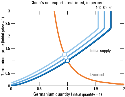
Graph showing germanium demand and supply curves for the rest of the world at different levels of restriction of China’s net exports of germanium for the baseline case.
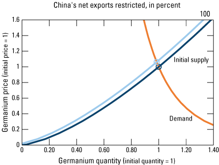
Graph showing germanium demand and supply curves for the rest of the world at different levels of restriction of China’s net exports of germanium for the low-impact case.
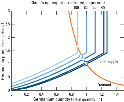
Graph showing germanium demand and supply curves for the rest of the world at different levels of restriction of China’s net exports of germanium for the high-impact case.
References Cited
360 Research Reports, 2022, Global semiconductor radiation detector market research report 2022: 360 Research Reports, 86 p., accessed August 1, 2023, at https://www.360researchreports.com/global-semiconductor-radiation-detector-market-20049118.
Air Liquide Advanced Materials, 2015, Germane: Air Liquide Advanced Materials, 1 p., accessed July 23, 2024, at https://electronics.airliquide.com/sites/electronics/files/germane_geh4_11_13_15.pdf.
Asian Metals Ltd., 2021, Germanium industry annual report 2020: Asian Metals Ltd., 22 p., accessed June 21, 2023, at https://www.asianmetal.com/news/data/1650691/6. [Report is available by subscription only.]
Asian Metals Ltd., 2023a, Gallium industry annual report 2022: Asian Metals Ltd., 23 p., accessed March 12, 2024, at https://www.asianmetal.com/news/1908632/Gallium-Industry-Annual-Report-2022/13.
Asian Metals Ltd., 2023b, Germanium industry annual report 2022: Asian Metals Ltd., 24 p., accessed March 12, 2024, at https://www.asianmetal.com/news/1908289/Germanium-Industry-Annual-Report-2022. [Report is available by subscription only.]
Bell Labs-Lucent Technologies, 1997, Bell Labs innovative germanium-recovery process is economically, environmentally friendly: Science Daily, October 23, accessed July 23, 2024, at https://www.sciencedaily.com/releases/1997/10/971023172421.htm.
Board of Governors of the Federal Reserve System, 2024, Industrial production—Manufacturing (NAICS) [IPMAN]: Federal Reserve System web page, accessed July 3, 2024, at https://fred.stlouisfed.org/series/IPMAN.
Bureau of Economic Analysis, 2023, GDP by industry: U.S. Bureau of Economic Analysis interactive data tables, accessed July 30, 2024, at https://www.bea.gov/itable/gdp-by-industry.
Business Research Insights, 2024, BGO crystal market size, share, growth and industry analysis by type (Czochralski method, and Bridgman method), by application (nuclear medicine (PET & CT, etc.), high energy physics, nuclear physics, space physics, and others), regional forecast to 2031: Business Research Insights BRI100472, 110 p., accessed May 23, 2024, at https://www.businessresearchinsights.com/market-reports/bgo-crystal-market-100472.
Butterman, W.C., and Carlin, J.F., 2004, Mineral commodity profiles—Antimony: U.S. Geological Survey Open-File Report 2003–0019, 35 p., accessed July 23, 2024, at https://doi.org/10.3133/ofr0319.
Butterman, W.C., and Jorgenson, J.D., 2005, Mineral commodity profiles—Germanium: U.S. Geological Survey Open-File Report 2004–1218, 22 p., accessed July 23, 2024, at https://doi.org/10.3133/ofr20041218.
Clouet, A., 2023, The thermal imaging and sensing market: Yole Intelligence, 20 p., accessed July 23, 2024, at https://medias.yolegroup.com/uploads/2023/05/spie-dcs-thermal.pdf.
Commission on Isotopic Abundances and Atomic Weights and International Union of Pure and Applied Chemistry, 2021, Standard atomic weights: Commission on Isotopic Abundances and Atomic Weights web page, accessed August 21, 2024, at https://www.ciaaw.org/atomic-weights.htm.
DeMarines, R., and Botwin, B., 2006, Defense industrial base assessment—U.S. imaging and sensors industry: U.S. Department of Commerce, 188 p., accessed July 23, 2024, at https://www.bis.doc.gov/index.php/documents/technology-evaluation/72-u-s-imaging-and-sensors-industry-2006/file.
Ditzen, J., Karavias, Y., and Westerlund, J., 2021, Testing and estimating structural breaks in time series and panel data in stata: Econometrics, article 14550, 27 p., accessed August 6, 2024, at https://doi.org/10.48550/arXiv.2110.14550.
Dobrzyński, D., Boguszewska-Czubara, A., and Sugimori, K., 2018, Hydrogeochemical and biomedical insights into germanium potential of curative waters—A case study of health resorts in the Sudetes Mountains (Poland): Environmental Geochemistry and Health, v. 40, no. 4, p. 1355–1375, accessed March 3, 2023, at https://doi.org/10.1007/s10653-017-0061-0.
Epic-Crystal, 2024, BGO scintillation crystal: Epic Scintillator web page, accessed July 23, 2024, at https://www.epic-scintillator.com/BGO-crystal-scintillator.
Feldman, D., Zuboy, J., Dummit, K., Stright, D., Heine, M., Mirletz, H., and Margolis, R., 2024, Winter 2024 solar industry update: National Renewable Energy Laboratory, 60 p., accessed July 23, 2024, at https://www.nrel.gov/docs/fy24osti/88780.pdf.
Fink, D.A., and Culver-Hopper, J., 1991, Germanium requirements for national defense: Institute for Defense Analyses Paper P–2606, 53 p., accessed July 23, 2024, at https://apps.dtic.mil/sti/tr/pdf/ADA240992.pdf.
Future Markets Insights, 2016, Global positron emissions tomography (PET) scanners market is estimated to expand at a CAGR of 4.7 percent by 2026: PR Newswire, October 11, accessed October 12, 2023, at https://www.prnewswire.com/news-releases/global-positron-emission-tomography-pet-scanners-market-is-estimated-to-expand-at-a-cagr-of-47-by-2026-596659 671.html.
Geological Survey of Finland, 2016, Metals and minerals production 2011–2015: Geological Survey of Finland data, accessed August 6, 2024, at https://web.archive.org/web/20190103053813/http://en.gtk.fi/informationservices/mineralproduction/finmipr1116.html.
Global Industry Analysts Inc, 2024, Global silicon germanium materials & devices market: Global Industry Analysts Inc., 287 p., accessed March 1, 2024, at https://www.researchandmarkets.com/reports/1206726/silicon_germanium_materials_and_devices_global.
Grand View Research, 2014, Radiation detection, monitoring and safety market size, share & trends analysis report by product (personal dosimeters, area process monitors), by detection type, by end-use, by region, and segment forecasts, 2018–2024: Grand View Research GVR–1–68038–239–6, 100 p., accessed August 1, 2024, at https://www.grandviewresearch.com/industry-analysis/radiation-detection-monitoring-and-safety-market.
Grand View Research, 2015, IR camera market size, share & trends analysis report by material (germanium, silicon, zinc selenide, sapphire), by application (military & defense, industrial, commercial, medical imaging) and segment forecasts to 2020: Grand View Research 978–1–68038–318–8, 105 p., accessed July 23, 2024, at https://www.grandviewresearch.com/industry-analysis/ir-infrared-camera-market.
Grand View Research, 2019, Fiber optics market size, share & trends analysis report by type (single mode, multi-mode, plastic optical fiber (POF)), by application (telecom, medical, oil & gas), by region, and segment forecasts, 2023–2030: Grand View Research GVR–1–68038–860–2, 100 p., accessed July 1, 2023, at https://www.grandviewresearch.com/industry-analysis/fiber-optics-market.
Grand View Research, 2022, PET scanners market size, share & trends analysis by modality (PET–CT, PET–MRI), by application (oncology, cardiology, neurology, others), by end-use, by region, and segment forecasts, 2023–2030: Grand View Research GVR–4–68040–040–9, 130 p., accessed August 1, 2023, at https://www.grandviewresearch.com/industry-analysis/pet-scanners-market-report.
Grand View Research, 2023, Fiber optic preform market size, share & trends analysis report by process (OVD, VAD, PCVD, MCVD), by product type (single-mode, multi-mode, plastic optical fiber), by end-user, by region, and segment forecasts, 2023–2030: Grand View Research GVR–2–68038–817–6, 100 p., accessed December 18, 2023, at https://www.grandviewresearch.com/industry-analysis/fiber-optic-preform-market.
Grohol, M., and Veeh, C., 2023, Study on the critical raw materials for the EU—2023—Final report: European Commission Directorate-General for Internal Market, Industry, Entrepreneurship and SMEs, 152 p., accessed July 30, 2024, at https://doi.org/10.2873/725585.
Guberman, D.E., 2011, Germanium, in Metals and minerals: U.S. Geological Survey Minerals Yearbook 2009, v. I, p. 30.1–30.8, accessed July 23, 2024, at https://www.usgs.gov/centers/national-minerals-information-center/germanium-statistics-and-information.
Guberman, D.E., 2013, Germanium, in Metals and minerals: U.S. Geological Survey Minerals Yearbook 2011, v. I, p. 30.1–30.7, accessed July 23, 2024, at https://www.usgs.gov/centers/national-minerals-information-center/germanium-statistics-and-information.
Guberman, D.E., 2016, Germanium, in Metals and minerals: U.S. Geological Survey Minerals Yearbook 2014, v. I, p. 30.1–30.7, accessed July 23, 2024, at https://www.usgs.gov/centers/national-minerals-information-center/germanium-statistics-and-information.
Horowitz, K.A., Remo, T.W., Smith, B., and Ptak, A.J., 2018, A techno-economic analysis and cost reduction roadmap for III-V solar cells: National Renewable Energy Laboratory, 35 p., accessed July 23, 2024, at https://doi.org/10.2172/1484349.
ImportGenius, 2024, Global trade data: ImportGenius data, accessed July 23, 2024, at https://www.importgenius.com/.
International Energy Agency, 2023a, International resource strategy—National stockpiling system: International Energy Agency web page, accessed January 3, 2024, at https://www.iea.org/policies/16639-international-resource-strategy-national-stockpiling-system.
International Energy Agency, 2023b, The strategy for securing reliable critical minerals: International Energy Agency web page, accessed January 3, 2024, at https://www.iea.org/policies/17942-the-strategy-for-securing-reliable-critical-minerals-supply.
Japan Organization for Metals and Energy Security, 2023, Mineral resources material flow 2022—Germanium (Ge) [in Japanese]: Japan Organization for Metals and Energy Security, 11 p., accessed January 2, 2024, at https://mric.jogmec.go.jp/wp-content/uploads/2023/10/material_flow2022_Ge.pdf.
Japan Organization for Metals and Energy Security, 2024, Mineral resources material flow 2022—Gallium (Ga) [in Japanese]: Japan Organization for Metals and Energy Security, 9 p., accessed December 2, 2023, at https://mric-jogmec-go-jp.translate.goog/wp-content/uploads/2024/01/material_flow2022_Ga.pdf.
Jaskula, B.W., 2021, Gallium, in Metals and minerals: U.S. Geological Survey Minerals Yearbook 2018, v. I, p. 27.1–27.9, accessed July 22, 2024, at https://www.usgs.gov/centers/national-minerals-information-center/gallium-statistics-and-information.
Jorgenson, J.D., 2006, Germanium recycling in the United States in 2000, chap. V of Sibley, S.F., ed., Flow studies for recycling metal commodities in the United States: U.S. Geological Survey Circular 1196, p. V1–V10, accessed July 23, 2024, at https://doi.org/10.3133/cir1196V.
Kelly, T.D., and Matos, G.R., 2023, Historical statistics for mineral and material commodities in the United States: U.S. Geological Survey, accessed January 2, 2024, at https://www.usgs.gov/centers/national-minerals-information-center/historical-statistics-mineral-and-material-commodities.
Lamb, G., 2022, Global PET resin capacity and projects: CZ Insights web page, accessed July 23, 2024, at https://www.czapp.com/explainers/global-pet-resin-capacity-and-projects/.
Lauri, L.S., 2019, Fennoscandia mineral potential for critical raw materials: Business Finland, [unpaginated], accessed June 23, 2022, at https://tapahtumat.tekes.fi/uploads/7c590795/Laura_Lauri-6001.pdf.
Lee, H., 2010, Germane gas production from germanium byproducts or impure germanium compounds: U.S. Patent and Trademark Office patent application US 2010/0183500 A1, 5 p., accessed July 23, 2024, at https://patentimages.storage.googleapis.com/f1/07/cd/a39ec221030897/US20100183500A1.pdf.
Licht, C., Peiró, L.T., and Villalba, G., 2015, Global substance flow analysis of gallium, germanium, and indium—Quantification of extraction, uses, and dissipative losses within their anthropogenic cycles: Journal of Industrial Ecology, v. 19, p. 890–903, accessed July 23, 2024, at https://doi.org/10.1111/jiec.12287.
Løvik, A.N., Restrepo, E., and Müller, D.B., 2015, The global anthropogenic gallium system—Determinants of demand, supply and efficiency improvements: Environmental Science & Technology, v. 49, p. 5704–5712, accessed July 23, 2024, at https://doi.org/10.1021/acs.est.5b00320.
Luxium Solutions, 2022, BGO scintillation material: Luxium Solutions web page, accessed July 23, 2024, at https://luxiumsolutions.com/radiation-detection-scintillators/crystal-scintillators/bgo-bismuth-germanate.
Market Research Future, 2023, Global compound semiconductor market overview: Market Research Future, accessed January 2, 2024, at https://www.marketresearchfuture.com/reports/compound-semiconductor-market-10129.
MarketsandMarkets Research Pvt. Ltd., 2023a, Compound semiconductor market: MarketsandMarkets Research Pvt. Ltd., accessed January 23, 2024, at https://www.marketsandmarkets.com/Market-Reports/compound-semiconductor-market-178858112.html.
MarketsandMarkets Research Pvt. Ltd., 2023b, Infrared imaging market size, share & industry trends analysis report by technology (cooled & uncooled infrared imaging), wavelength (near, shortwave, mid-wave, & long-wave infrared), application (security & surveillance, monitoring & inspection, detection), vertical—Global forecast to 2028: MarketsandMarkets Research Pvt. Ltd. report, 218 p., accessed October 23, 2021, at https://www.marketsandmarkets.com/Market-Reports/infrared-IR-sensing-imaging-market-593.html.
Maximize Market Research Pvt. Ltd., 2023, Compound semiconductor market—Global overlook of industry and forecast (2023–2029): Maximize Market Research Pvt. Ltd., accessed March 1, 2024, at https://www.maximizemarketresearch.com/market-report/global-compound-semiconductor-market/28695/.
McCarthy, D., 2022, DOE SBIR–STTR program success story: U.S. Department of Energy, 3 p., accessed August 1, 2023, at https://science.osti.gov/-/media/sbir/pdf/Success-Stories/2022/20221107-PHDS-Co---FINAL.pdf.
Melcher, F., and Buchholz, P., 2014, Germanium, in Gunn, G., ed., Critical metals handbook. John Wiley & Sons, Ltd., p. 177–203., https://doi.org/10.1002/9781118755341.ch8.
Ministry of Commerce and General Administration of Customs (China), 2023, Implementation of Export controls on gallium- and germanium-related items [in Chinese]: Ministry of Commerce and the General Administration of Customs announcement 23 accessed October 2, 2023, http://www.mofcom.gov.cn/article/zwgk/gkzcfb/202307/20230703419666.shtml.
Mirion Technologies Inc, 2023, Gamma and x-ray detection: Mirion Technologies Inc. web page, accessed August 1, 2023, at https://www.mirion.com/discover/knowledge-hub/articles/education/nuclear-measurement-fundamental-principle-gamma-and-x-ray-detection.
Neo Performance Materials, 2023, Fast forwarding the clean energy transition as a global leader in rare earth magnetics & critical materials: Neo Performance Materials presentation, 38 p., accessed June 2, 2024, at https://web.archive.org/web/20240203232243/https://www.neomaterials.com/wp-content/uploads/2024/01/Neo_Investor_Presentation.pdf.
Ohlmann, J., Winter, E., Schön, J., Dold, P., Henatsch, O., Khaan, A.A., Nold, S., and Lackner, D., 2023, GeSiR final project meeting: Fraunhofer ISE, 42 p., accessed July 23, 2024, at https://nebula.esa.int/sites/default/files/neb_tec_studies/3018/public/GeSiR FP 2023_03.pdf.
Pesaran, M.H., and Shin, Y., 1999, Autoregressive distributed lag modelling approach to cointegration analysis, chap. 11 of Econometric methods, part V of Strøm, S., ed., Econometrics and economic theory in the 20th century: Econometric Society Monograph 31, p. 371–413, accessed August 7, 2024, at https://doi.org/10.1017/CCOL521633230.011.
Pesaran, M.H., Shin, Y., and Smith, R.J., 2001, Bounds testing approaches to the analysis of level relationships: Journal of Applied Econometrics, v. 16, p. 289–326. https://doi.org/10.1002/jae.616.
PHDS Co, 2023, GeGl imaging HPGe detector: PHDS Co. web page, accessed August 1, 2023, at https://phdsco.com/products/gegi.
Polaris Market Research, 2023, Compound semiconductor market share, size, trends, industry analysis report, by product (LED, optoelectronics, RF devices, power electronics, diode, bare die, module, and others); by application; by type; by region; segment forecast, 2023–2032: Polaris Market Research, 118 p., accessed December 12, 2023, at https://www.polarismarketresearch.com/industry-analysis/compound-semiconductor-market.
Precedence Research Pvt. Ltd., 2023, Compound semiconductor market by deposition technology—molecular beam epitaxy, CVD, ammonothermal, hydride vapor phase epitaxy, atomic layer deposition, and others; by type—II–VI compound semiconductors, III–V compound semiconductors, IV–IV compound semiconductors, sapphire, and others; by product—transistors, power semiconductor, diodes & rectifiers, integrated circuits and others; by application—global market size, share, growth, trends analysis, segment forecasts, regional outlook 2023–2032: Precedence Research Pvt. Ltd., 150 p., accessed March 2, 2024, at https://www.precedenceresearch.com/compound-semiconductor-market.
Project Blue Group Ltd., 2023, Gallium market service: Project Blue Group Ltd. web page, accessed August 7, 2024, at https://projectblue.com/subscriptions/critical-materials/gallium.
QY Research, 2019, Global infrared lens market research report 2019: Trusted Business Insights report, 90 p., accessed October 19, 2023, at https://www.trustedbusinessinsights.com/details/tbiqyr24759-global-infrared-lens-ir-lens-market-research-report-2019.
QY Research, 2022, Global electronic special germane (GeH4) market research report 2022: QY Research, 126 p., accessed March 2, 2023, at https://www.giiresearch.com/report/qyr1104922-global-electronic-special-germane-geh4-market.html.
Reece, B., 2022, DLA program introduces domestic germanium recycling capability: Defense Logistics Agency news, June 29, accessed November 4, 2023, at https://www.defense.gov/News/News-Stories/Article/Article/3079217/dla-program-introduces-domestic-germanium-recycling-capability/.
Reichl, C., and Schatz, M., 2023, World mining data 2023: Austrian Ministry of Finance, 265 p., accessed July 23, 2024, at https://www.world-mining-data.info/wmd/downloads/PDF/WMD2023.pdf.
Risk & Policy Analysis Ltd., 2012, Stockpiling of non-energy raw materials: European Commission Directorate-General Enterprise and Industry, final report, Risk & Policy Analysis Ltd., [variously paginated], accessed August 7, 2024, at https://docslib.org/doc/10354616/stockpiling-of-non-energy-raw-materials.
Rongguo, C., Juan, G., Liwen, Y., Huy, D., and Liedtke, M., 2016, Supply and demand of lithium and gallium: Information Center of Ministry of Land and Resources and Bundesanstalt für Geowissenschaften und Rohstoffe, 50 p., accessed August 7, 2024, at https://www.bgr.bund.de/EN/Themen/Min_rohstoffe/Downloads/studie_Li_Ga.pdf?__blob=publicationFile.
Rowe, S., 2024, What optical materials work best in the IR (infrared)?: Esco Optics, July 2, accessed July 23, 2024, at https://escooptics.com/blogs/news/what-optical-materials-work-best-in-the-ir-infrared.
Shanks, W.C.P., III, Kimball, B.E., Tolcin, A.C., and Guberman, D.E., 2017, Germanium and indium, chap. I of Schulz, K.J., DeYoung, J.H., Jr., Seal, R.R., II, and Bradley, D.C., eds., Critical mineral resources of the United States—Economic and environmental geology and prospects for future supply: U.S. Geological Survey Professional Paper 1802, p. I1–I27, accessed July 23, 2024, at https://doi.org/10.3133/pp1802.
Shojaeddini, E., Alonso, E., and Nassar, N.T., 2024, Estimating price elasticity of demand for mineral commodities used in lithium-ion batteries in the face of surging demand: Resources, Conservation, and Recycling, v. 207, paper 107664, 9 p., accessed July 23, 2024, at https://doi.org/10.1016/j.resconrec.2024.107664.
Sterlite Technologies Ltd., 2023, Earnings call Q4 FY23: Sterlite Technologies Ltd. Earnings presentation, 44 p., accessed December 21, 2023, at https://stl.tech/wp-content/uploads/2023/05/Earnings_Presentation_Q4_FY23_vf.pdf.
Stolyarov, G., Lyrchikova, A., Gordeyeva, M., Devitt, P., Trevelyan, M., and Neely, J., 2023, Russia’s Rostec says ready to boost germanium output for domestic market: Reuters, July 5, accessed September 23, 2023, at https://www.reuters.com/article/russia-metals/update-1-russias-rostec-says-ready-to-boost-germanium-output-for-domestic-market-idUKL1N38R15L/.
Thomas, C.L., 2023, Germanium, in Metals and minerals: U.S. Geological Survey Minerals Yearbook 2018, v. I, p. 30.1–30.8, accessed July 30, 2024, at https://www.usgs.gov/centers/national-minerals-information-center/germanium-statistics-and-information.
U.S. Census Bureau, 2017a, EC1700NAPCSINDPRD—All sectors—Industry by products for the U.S. and states—2017: U.S. Census Bureau data, accessed July 23, 2024, at https://data.census.gov/table/ECNNAPCSIND2017.EC1700NAPCSINDPRD?q=economic census.
U.S. Census Bureau, 2017b, NAICS sector 31–33—Manufacturing: U.S. Census Bureau data, accessed December 5, 2023, at https://www.census.gov/data/tables/2017/econ/economic-census/naics-sector-31-33.html.
U.S. Census Bureau, 2022, 2018–2021 annual survey of manufactures: U.S. Census Bureau data, accessed October 11, 2023, at https://www.census.gov/data/tables/time-series/econ/asm/2018-2021-asm.html.
U.S. Environmental Protection Agency, 2020, TSCA chemical data report fact sheet—Reporting thresholds: U.S. Environmental Protection Agency, 4 p., accessed October 13, 2023, at https://www.epa.gov/sites/default/files/2020-05/documents/fact_sheet_reporting_thresholds_04.28.2020.pdf.
U.S. Environmental Protection Agency, 2023, Chemical data reporting: U.S. Environmental Protection Agency data, accessed January 2, 2024, at https://www.epa.gov/chemical-data-reporting/access-cdr-data.
U.S. Geological Survey, 2013, Metal prices in the United States through 2010: U.S. Geological Survey Scientific Investigations Report 2012–5188, 206 p., accessed June 23, 2024, at https://doi.org/10.3133/sir20125188.
U.S. Geological Survey, 2024, Mineral commodity summaries 2024: U.S. Geological Survey, 212 p., https://doi.org/10.3133/mcs2024.
U.S. International Trade Commission, 2024, Harmonized tariff schedule [2024 HTS revision 7]: U.S. International Trade Commission data, accessed August 8, 2024, at https://hts.usitc.gov/.
Umicore, 2021, Pioneering the sourcing and recycling of sustainable germanium: Umicore news, accessed March 19, 2021, at https://www.umicore.com/en/newsroom/pioneering-the-sourcing-and-recycling-of-sustainable-germanium/.
Umicore, 2022, Effective use of Ge: Umicore presentation, 25 p., accessed July 23, 2024, at https://nebula.esa.int/sites/default/files/neb_tec_studies/2653/public/4000128156_FP.pdf.
Verified Market Research, 2023, Compound semiconductor market size by seat type (bucket seats, bench seats), by material (fabric seats, leather seats, synthetic seats), by vehicle type (passenger cars, commercial vehicles, sports utility vehicles (SUVs)), by geographic scope and forecast: Verified Market Research, 202 p., accessed February 3, 2024, at https://www.verifiedmarketresearch.com/product/compound-semiconductor-market/.
Voltaix, 2010, Voltaix currents: Voltaix newsletter, 8 p., accessed January 3, 2013, at http://208.106.232.250/images/news/newsletter_06_10.pdf. [Document not available online at time of publication.]
Wilson, G.M., Al-Jassim, M., Metzger, W.K., Glunz, S.W., Verlinden, P., Xiong, G., Mansfield, L.M., Stanbery, B.J., Zhu, K., Yan, Y., Berry, J.J., Ptak., A.J., Dimroth, F., Kayes, B.M., Tamboli, A.C., Peibst, R., Catchpole, K., Reese, M.O., Klinga, C.S., Denholm, P., Morjaria, M., Deceglie, M.G., Freeman, J.M., Mikofski, M.A., Jordan, D.C., TamizhMani, G., and Sulas-Kern, D.B., 2020, The 2020 photovoltaic technologies roadmap: Journal of Physics D: Applied Physics, v. 53, no. 49, article 493001, 47 p., accessed July 23, 2024, at https://doi.org/10.1088/1361-6463/ab9c6a.
World Bank Group, 2023a, GDP (constant 2015 US$): World Bank Publications world development indicators web page, accessed July 23, 2023, at https://data.worldbank.org/indicator/NY.GDP.MKTP.KD.
World Bank Group, 2023b, GDP (current US$): World Bank Publications world development indicators web page, accessed July 23, 2023, at https://data.worldbank.org/indicator/NY.GDP.MKTP.CD.
World Semiconductor Trade Statistics GmbH, 2022, Fall 2022 forecast: World Semiconductor Trade Statistics GmbH web page, accessed October 12, 2023, at https://www.wsts.org/76/103/WSTS-Semiconductor-Market-Forecast-Fall-2022.
World Customs Organization, 2023, Harmonized system: World Customs Organization database, accessed August 8, 2024, at https://www.wcotradetools.org/en/harmonized-system.
Zen Innovations, A.G., 2024, Global trade tracker: Zen Innovations AG database, accessed January 23, 2024, at https://www.globaltradetracker.com/.
Abbreviations
AlGaAs
aluminum gallium arsenide
BEA
Bureau of Economic Analysis
BGO
bismuth germanium oxide
CDR
Chemical Data Reporting [database]
CIGS
copper indium gallium diselenide
DC
direct current
EPA
U.S. Environmental Protection Agency
GaAs
gallium arsenide
GaN
gallium nitride
GDP
gross domestic product
GeCl4
germanium tetrachloride
GeH4
germane gas
GeO2
germanium oxide
HS
Harmonized Commodity Description and Coding System
HTS
Harmonized Tariff Schedule of the United States
InAs
indium arsenide
InP
indium phosphide
InSb
indium antimonide
IO
input-output
LED
light-emitting diode
lidar
light detection and ranging
NAICS
North American Industry Classification System
NAPCS
North American Product Classification System
NdFeB
neodymium-iron-boron
PET
polyethylene terephthalate
PV
photovoltaic
RF
radio frequency
SiGe
silicon germanium
USGS
U.S. Geological Survey
WLAN
wireless local-area network
ZrO2
zirconium oxide
For more information, contact
Director, National Minerals Information Center
U.S. Geological Survey
12201 Sunrise Valley Drive
988 National Center
Reston, VA 20192
https://www.usgs.gov/centers/national-minerals-information-center
Publishing support provided by the Pembroke and Reston Publishing Service Centers
Disclaimers
Any use of trade, firm, or product names is for descriptive purposes only and does not imply endorsement by the U.S. Government.
Although this information product, for the most part, is in the public domain, it also may contain copyrighted materials as noted in the text. Permission to reproduce copyrighted items must be secured from the copyright owner.
Suggested Citation
Nassar, N.T., Shojaeddini, E., Alonso, E., Jaskula, B., and Tolcin, A., 2024, Quantifying potential effects of China’s gallium and germanium export restrictions on the U.S. economy: U.S. Geological Survey Open-File Report 2024–1057, 66 p., https://doi.org/10.3133/ofr20241057.
ISSN: 2331-1258 (online)
| Publication type | Report |
|---|---|
| Publication Subtype | USGS Numbered Series |
| Title | Quantifying potential effects of China’s gallium and germanium export restrictions on the U.S. economy |
| Series title | Open-File Report |
| Series number | 2024-1057 |
| DOI | 10.3133/ofr20241057 |
| Publication Date | October 15, 2024 |
| Year Published | 2024 |
| Language | English |
| Publisher | U.S. Geological Survey |
| Publisher location | Reston, VA |
| Contributing office(s) | National Minerals Information Center |
| Description | vi, 66 p. |
| Online Only (Y/N) | Y |
| Additional Online Files (Y/N) | N |