

U.S. Geological Survey Karst Interest Group Proceedings, Nashville, Tennessee, October 22-24, 2024
Links
- Document: Report (5.85 MB pdf) , HTML , XML
- Related Work: Scientific Investigations Report 2020–5019 - U.S. Geological Survey Karst Interest Group Proceedings, October 19–20, 2021
- NGMDB Index Pages:
- A national model of sinkhole susceptibility in karst and pseudokarst areas of the conterminous United States (html)
- The geologic framework of karst in Monroe County, West Virginia: a tale of two systems (html)
- A karst-rich impact crater: drill cores from the Flynn Creek crater, north-central Tennessee (html)
- Planned alternative water supply technologies utilizing the karst aquifers of Texas (html)
- Geophysical characterization of glacially influenced, submature karst drainage features in western New York (html)
- Modern cave monitoring informs interpretations of past climate change: applications to Titan cave, Wyoming (html)
- Results of tracer testing at Pah Tempe Hot Springs, Hurricane, Utah (html)
- Download citation as: RIS | Dublin Core
Introduction3
Karst hydrogeologic systems represent challenging and unique conditions to scientists studying groundwater flow and contaminant transport. The distinctive hydrology and terrains that form from the dissolution and erosional processes of carbonate rocks (primarily limestone and dolomite) and evaporites (gypsum, anhydrite, and halite) define karst aquifer systems that are present throughout the world. Karst aquifer systems are complex; they result from past depositional environments, post-depositional tectonic events, and diagenetic and weathering processes. These factors involve biological, chemical, and physical changes that, when combined with the diverse climatic regions in which karst development can occur, result in the unique dual- or triple-porosity nature of karst aquifers.
Karst terrains are characterized by distinct and beautiful landscapes, caverns, and springs, and many of the exceptional karst areas are designated as national or state parks. In addition, there are numerous caves on public and private lands that have been developed commercially. Both public and private properties can provide access for scientists to study the flow of groundwater and characteristics of the aquifer in caves. Likewise, the range and complexity of landforms and groundwater flow systems associated with karst terrains are enormous, perhaps more than any other aquifer type. Karst aquifers and landscapes that form in tropical areas, such as the cockpit karst along the north coast of Puerto Rico, differ greatly from karst landforms in more arid climates, such as the Edwards Plateau in west-central Texas or the Guadalupe Mountains near Carlsbad, New Mexico, where hypogenic processes have played a major role in speleogenesis. Caves, aquifers, and springs support a variety of unique flora and fauna, many of which are listed as federally endangered species. Understanding karst hydrology is vital for protecting these ecosystems. As a result, numerous Federal, State, and local agencies have a strong interest in the study of karst terrains.
In addition, most of the major springs and aquifers in the United States are developed in carbonate rocks associated with karst, such as the Floridan aquifer system in Florida and parts of Alabama, Georgia, and South Carolina; the Ozark Plateaus aquifer system in parts of Arkansas, Kansas, Missouri, and Oklahoma; and the Edwards-Trinity aquifer system in west-central Texas. These aquifers, and the springs that discharge from them, serve as major water-supply sources. Competition for the water resources of karst aquifers is common, and urban development and the lack of attenuation of contaminants in karst areas due to dissolution features that form direct pathways into karst aquifers can affect the ecosystem and water quality associated with these aquifers.
The concept for developing a platform for interaction among scientists within the U.S. Geological Survey (USGS) working on karst-related studies began at the November 1999 National Groundwater Meeting of the USGS. The resulting Karst Interest Group (KIG) formed in 2000, and is a loosely knit, grass-roots organization of USGS and non-USGS scientists and researchers devoted to fostering better communication among scientists working on or interested in, karst science. The primary mission of the KIG is to encourage and support interdisciplinary collaboration and technology transfer among scientists working in karst areas. The KIG encourages collaborative studies between the different mission areas of the USGS, as well as with other Federal and State agencies and researchers from academia and institutes. To accomplish its mission, the KIG has organized a series of workshops that have been held near nationally important karst areas. To date (2024), nine KIG workshops, including the workshop documented in this report, have been held. The workshops have included oral and poster sessions on selected karst-related topics and research, as well as field trips to local karst areas. To increase non-USGS participation, an effort was made for the workshops to be held at a university or institute beginning with the fourth workshop. Proceedings of the workshops are published by the USGS and are available online at the USGS Publications Warehouse (https://pubs.er.usgs.gov/) by using the search term “karst interest group.”
3Note these “Introduction” and “Acknowledgments” sections are modified from the previous Karst Interest Group proceedings: Kuniansky (2001), Kuniansky (2002), Kuniansky (2005), Kuniansky (2008), Kuniansky (2011), Kuniansky and Spangler (2014), Kuniansky and Spangler (2017), and Kuniansky and Spangler (2021). Citations above will be provided after the “Acknowledgments” section.
Acknowledgments3
The first KIG workshop was held in St. Petersburg, Florida, in 2001, near the large springs and other karst features of the Floridan aquifer system, with Lari Knochenmus, Ann Tihansky, and Peter Schwarzenski as local coordinators (Kuniansky, 2001). The second KIG workshop was held in 2002, in Shepherdstown, West Virginia, in proximity to the carbonate aquifers of the northern Shenandoah Valley and was highlighted by an invited presentation on karst literature by the late Barry F. Beck of P.E. LaMoreaux and Associates, with local coordinators David Nelms, David Weary, and Randall Orndorff (Kuniansky, 2002). The third KIG workshop was held in 2005, in Rapid City, South Dakota, near evaporite karst features in limestones of the Madison Group in the Black Hills of South Dakota, with Jack Epstein (field trips), Larry Putnam, and Andy Long as local coordinators (Kuniansky, 2005). The Rapid City KIG workshop included field trips to Wind Cave National Park (Rod Horrocks, National Park Service [NPS] guide) and Jewel Cave National Monument (Mike Wiles, NPS guide), and featured a presentation by Thomas Casadevall, then USGS Central Region Director, on the status of earth science at the USGS. The fourth KIG workshop in 2008 was hosted by the Hoffman Environmental Research Institute and Center for Cave and Karst Studies at Western Kentucky University in Bowling Green, Kentucky, near Mammoth Cave National Park and karst features of the Chester Upland and Pennyroyal Plateau, with Chris Groves, Western Kentucky University, as the local coordinator and field trip guide (Kuniansky, 2008). The workshop featured a late-night field trip into Mammoth Cave led by Rickard Toomey and Rick Olsen of the National Park Service.
The fifth KIG workshop took place in Fayetteville, Arkansas, in 2011, and was a joint meeting of the USGS KIG and University of Arkansas’ (UA) HydroDays workshop, hosted by the Department of Geosciences at the UA with Van Brahana, UA, as local coordinator and field trip guide (Kuniansky, 2011). The workshop featured a field trip to the unique karst terrain along the Buffalo National River in the southern Ozarks, and a keynote presentation on paleokarst in the United States was delivered by Art and Peggy Palmer. The sixth KIG workshop was hosted by the National Cave and Karst Research Institute (NCKRI) in 2014, in Carlsbad, New Mexico. George Veni, Director of the NCKRI, served as a co-chair of the workshop with Eve L. Kuniansky of the USGS (Kuniansky and Spangler, 2014). The workshop featured speaker Dr. Penelope Boston, Director of Cave and Karst Studies at New Mexico Tech-Socorro and Academic Director at the NCKRI, who addressed the future of karst research. The field trip on evaporite karst of the lower Pecos Valley was led by Lewis Land (NCKRI karst hydrologist), and the field trip on the geology of Carlsbad Caverns National Park was led by George Veni.
The seventh KIG workshop was held in San Antonio in 2017 at the University of Texas at San Antonio (UTSA). The workshop was hosted by the Department of Geological Sciences Student Geological Society (SGS), and student chapters of the American Association of Petroleum Geologists (AAPG) and Association of Engineering Geologists (AEG), with support by the UTSA Department of Geological Sciences and Center for Water Research (Kuniansky and Spangler, 2017). Two organizations assisted the UTSA student chapters in hosting the meeting by donating funds to the chapters: the Edwards Aquifer Authority (EAA), San Antonio, Texas and the Barton Springs Edwards Aquifer Authority, Austin, Texas. Additionally, the UTSA Center for Water Research and Department of Geological Sciences helped develop sessions on cave and karst research in China for the workshop. The keynote speakers were George Veni (NCKRI) and Geary M. Schindel (EAA). The coordinators for the 2017 KIG workshop were Eve L. Kuniansky and Allan K. Clark of the USGS and Amy R. Clark and Alexis Godet from UTSA. The field trip, coordinated by Allan K. Clark and Amy R. Clark, highlighted current karst research occurring within the Edwards and Trinity karst systems and ended with viewing the bat flight out of Bracken Cave, where an estimated 15 to 20 million Mexican free-tailed bats roost during the summer months.
The eighth workshop was held virtually in 2021 with all presentations done as videos, with 5-minute live question-and-answer periods after each video (Kuniansky and Spangler, 2021). Originally, the 2020 KIG workshop was to be held in Nashville, Tennessee, hosted by Tennessee State University (TSU) but was postponed because of the coronavirus disease (COVID-19) pandemic, which prevented large gatherings of people. The planning committee for the eighth workshop included Eve L. Kuniansky (USGS, Emeritus), Lawrence E. Spangler (USGS, Emeritus), Allan K. Clark (USGS), Douglas J. Schnoebelen (USGS), Thomas D. Byl (USGS and TSU), and Benjamin V. Miller (USGS). The field trip guide to the Cumberland Plateau of Tennessee was prepared by Benjamin Miller and published in that proceedings, but not conducted (Kuniansky and Spangler, 2021).
The current (2024) and ninth KIG workshop is being held in Nashville, Tennessee, in person and hosted by TSU, with the same planning committee as in 2020 plus Laura DeMott (USGS, New York Water Science Center). The optional field trip to the Cumberland Plateau of Tennessee is led by Ben Miller and scheduled for Thursday, October 24. The planning committee for the KIG would like to thank Ramona Neafie (USGS) for her hard work updating the KIG website and Lynne Fahlquist (USGS) for her assistance in obtaining meeting approval. Additionally, Linzy Foster (USGS) is providing assistance at the workshop.
All abstracts had a minimum of two peer reviews and were edited for consistency of appearance. The use of trade, firm or product names is for descriptive purposes only and does not imply endorsement by the U.S. Government. The USGS Water Availability and Use Science Program funded the publication costs of the proceedings.
The organizers sincerely appreciate all the efforts of past and present workshop organizers and hope that this workshop continues to promote future collaboration among scientists of varied and diverse backgrounds and improves our understanding of karst aquifer systems in the United States and its territories.
Sincerely,
Allan K. Clark, USGS San Antonio, Texas; Eve L. Kuniansky, USGS, Norcross, Georgia; and Lawrence E. Spangler, USGS, Salt Lake City, Utah
References for Introduction and Acknowledgments
Kuniansky, E.L., 2001, ed., U.S. Geological Survey Karst Interest Group Proceedings, St. Petersburg, Florida, February 13–16, 2001: U.S. Geological Survey Water-Resources Investigations Report 01-4011, 211p., http://doi.org/10.3133/wri014011.
Kuniansky, E.L., 2002, ed., U.S. Geological Survey Karst Interest Group Proceedings, Shepherdstown, West Virginia, August 20–22, 2002: U.S. Geological Survey Water-Resources Investigations Report 02-4174, 89 p., https://pubs.usgs.gov/publication/wri024174.
Kuniansky, E.L., 2005, ed., U.S. Geological Survey Karst Interest Group Proceedings, Rapid City, South Dakota, September 12–15, 2005: U.S. Geological Survey Scientific Investigations Report 2005-5160, 296 p., https://doi.org/10.3133/sir20055160.
Kuniansky, E.L., 2008, ed., U.S. Geological Survey Karst Interest Group Proceedings, Bowling Green, Kentucky, May 27–29, 2008: U.S. Geological Survey Scientific Investigations Report 2008-5023, 142 p., https://doi.org/10.3133/sir20085023.
Kuniansky, E.L., 2011, ed., U.S. Geological Survey Karst Interest Group Proceedings, Fayetteville, Arkansas, April 26–29, 2011: U.S. Geological Survey Scientific Investigations Report 2011-5031, 212 p., https://doi.org/10.3133/sir20115031.
Kuniansky, E.L., and Spangler, L.E., 2014, eds., U.S. Geological Survey Karst Interest Group Proceedings, Carlsbad, New Mexico, April 29–May 2, 2014: U.S. Geological Survey Scientific Investigations Report 2014-5035, 155 p., http://dx.doi.org/10.3133/sir20145035.
Kuniansky, E.L., and Spangler, L.E., eds., 2017, U.S. Geological Survey Karst Interest Group Proceedings, San Antonio, Texas, May 16–18, 2017: U.S. Geological Survey Scientific Investigations Report 2017–5023, 245 p., https://doi.org/10.3133/sir20175023.
Kuniansky, E.L., and Spangler, L.E., eds., 2021, U.S. Geological Survey Karst Interest Group Proceedings, October 19–20, 2021: U.S. Geological Survey Scientific Investigations Report 2020–5019, 147 p., https://doi.org/10.3133/sir20205019.
Agenda
Karst Focused Ebooks of the Groundwater Project
Abstract
The Groundwater Project (GWP) is a global, volunteer-based, nongovernmental organization (NGO), initiated in 2017. It was started to help address the global freshwater crisis identified by both the United Nations and the United Nations Educational, Scientific and Cultural Organization (UNESCO). Sustainable use of groundwater may help address the crisis, especially in developing countries. The major goal of the GWP is to produce free online educational materials for many different audiences (lay people and students at multiple educational levels) and on many different groundwater-related topics. As of the end of 2023 there were 44 online educational publications on GWP web pages.
Karst aquifers serve as vital water resources for large populations, and the large springs typical of karst aquifers often support unique ecosystems. The complexity of karst aquifers is well known to the scientific community. There are currently (as of July 2024) three GWP online publications related to karst. Introduction to Karst Aquifers (Kuniansky and others, 2022) was the first karst related textbook published by the GWP. The audience for Kuniansky and others (2022) is upper-level undergraduate science and engineering students (for example, students in geology, earth science, hydrology, hydrogeology, water resources management, or civil and environmental engineering). The Edwards Aquifer (Sharp and Green, 2022) was the second book published about a very important karst aquifer system in Texas, United States of America. This online book describes how the Edwards aquifer functions as a hydrogeologic system by covering almost every topic in hydrogeology as it relates to this specific karst aquifer, including ecological and water resource management and regulation. The third book is titled Karst: Environment and Management of Aquifers, written by Zoran Stevanović, John Gunn, Nico Goldscheider, and Nataša Ravbar (Stevanović and others, 2024). The environment and management ebook is intended for a broad audience including readers without prior knowledge of groundwater science. The intent is to provide readers with a descriptive and comprehensive understanding of the complexity of karst and why specialized engineering is required for water resource management, prevention of aquifer contamination, conservation of ecosystems, and construction on karst terrain. This ebook also has an appendix that includes over 80 photographs of karst around the globe.
These first three karst related GWP books were shepherded through the publication process by Amanda Sills, Eileen Poeter, and John Cherry. If you are reading this abstract and interested in volunteering to publish karst related educational material for the GWP, feel free to contact Eve Kuniansky at elkunian@gmail.com.
References Cited
Kuniansky, E.L., Taylor C.J., Williams J.H., and Paillet, F., 2022, Introduction to karst aquifers: The Groundwater Project, Guelph, Ontario, Canada, https://doi.org/10.21083/978-1-77470-040-2.
Sharp, J.M., and Green, R.T., 2022, The Edwards aquifer: The Groundwater Project, Guelph, Ontario, Canada, https://doi.org/10.21083/978-1-77470-029-7.
Stevanović, Z., Gunn, J., Goldscheider, N., and Ravbar, N., 2024, Karst: Environment and management of aquifers: The Groundwater Project, Guelph, Ontario, Canada, https://gw-project.org/books/karst-environment-and-management-of-aquifers/ .
A National Model of Sinkhole Susceptibility in Karst and Pseudokarst Areas of the Conterminous United States
Abstract
Sinkholes are a characteristic landform of karst; thus, mapping of karst areas may include documenting the degree of sinkhole formation within the karst landscape. The ability to capture these closed depressions is tied to the availability of accurate digital elevation models (DEMs) for deriving topography. Using the national coverage of DEMs at 1/3 arc-second resolution (approximately 10 meters) and the development of computational methods to extract closed depressions from these elevation models, a national inventory of closed depressions in karst and pseudokarst regions was produced (Doctor and others, 2020; Jones and others, 2021). These data were then combined with nationally consistent data for factors related to geology, soils, precipitation extremes, and urban development to create a heuristic additive model of sinkhole susceptibility at 6-kilometer grid cell resolution within karst regions of the conterminous United States (Wood and others, 2023).
The resulting maps identify potential sinkhole hotspots based on current (2019) conditions and an estimated 50 years (2070–2079) into the future based on projected climate change and urban development scenarios (fig. 1). Areas characterized as having either high or very high sinkhole susceptibility contain 94–99 percent of already known or probable sinkhole locations from state databases for Tennessee, Missouri, and Kentucky. States and counties with the highest amounts and percentages of land in zones of highest sinkhole susceptibility were identified (fig. 2). These results provide a uniform index of sinkhole potential as a starting point for national-scale land use planning, in contrast to more localized assessments produced through various methods within individual States or smaller areas. Projected changes in extreme precipitation and development did not substantially change the locations of current hotspots of highest sinkhole susceptibility. Land use and human disturbance of natural hydrologic conditions are exacerbating factors to the natural conditions for sinkhole development that evolve over geologic time. These influences will likely have more impact on future sinkhole occurrence than hydrologic impacts resulting from projected climate change.
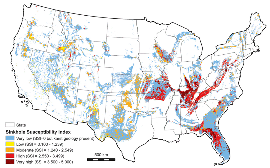
Map of Sinkhole Susceptibility Index (SSI) values by State based on current (2019) conditions. Additional information on data sources and analysis can be found in Wood and others (2023).
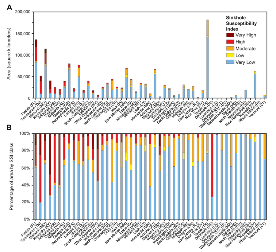
A, Amount of land (in square kilometers) by State in areas characterized by Sinkhole Susceptibility Index (SSI) values, assuming current (2019) conditions. B, Percentage of land area mapped with karst or pseudokarst geology by SSI values. States, with abbreviations in parentheses, are ordered on the x-axis from left to right by the total amount of land with SSI values that are either high or very high (Doctor and others, 2020).
References Cited
Doctor, D.H., Jones, J., Wood, N., Falgour, J., and Rapstine, N., 2020, Progress toward a preliminary karst depression density map for the conterminous United States, in Land, L., Kromhout, C., and Byle, M.J., eds., Proceedings of the 16th Multidisciplinary Conference on Sinkholes and the Engineering and Environmental Impacts of Karst: National Cave and Karst Research Institute Symposium 8, Carlsbad, NM, p. 315–326, https://doi.org/10.5038/9781733375313.1003.
Jones, J.M., Doctor, D.H., Wood, N.J., Falgout, J.T., and Rapstine, N.I., 2021, Closed depression density in karst regions of the conterminous United States—features and grid data: U.S. Geological Survey data release, https://doi.org/10.5066/P9EV2I12.
A Summary of Karst Regions in Tennessee
Abstract
“2Karst terrains are characteristic of much of the eastern two-thirds of Tennessee. The occurrence of karst features in Tennessee affects property development, infrastructure, water supply, contaminant transport, and flood and drought planning in Middle and East Tennessee. Karst aquifers in Tennessee provided close to 40 million gallons per day to public water systems in 2015 with the carbonate formations in the Valley and Ridge province of East Tennessee being the second most productive aquifer in the state. The interconnection between surface water and karst systems results in offstream flooding in Tennessee. Sinkhole collapse and the potential for sinkhole collapse have affected subdivisions in several regions in the State. The importance of karst resources to the hydrology and ecology of Tennessee has only been fully defined in relatively small areas. Additional work is needed to further evaluate karst features relative to public water supplies and susceptibility of the systems to contamination, the karst hydrology and ecology along the Cumberland Plateau escarpment, and impacts and controls of sinkhole flooding.”
2Extended abstract published in Bradley (2021).
Reference Cited
Bradley, M., 2021, A summary of karst regions in Tennessee, in Kuniansky, E.L., and Spangler, L.E., eds., 2021, U.S. Geological Survey Karst Interest Group Proceedings, October 19–20, 2021: U.S. Geological Survey Scientific Investigations Report 2020–5019, p. 18–30, accessed June 2024, at https://doi.org/10.3133/sir20205019.
Seepage Investigations in Wear Cove to Quantify Streamflow Gains and Losses in a Carbonate Fenster in the Western Great Smoky Mountains, Tennessee
Abstract
Karst landscapes can often create challenging environments for the planning and design of infrastructure because they are often both particularly susceptible to contamination from surface activities and serve as habitat for unique and sensitive biota. Because of these conditions, it is necessary to understand the characteristics of a karst environment in order to better preserve water quality and prevent degradation of subterranean ecosystems. Wear Cove is a carbonate fenster (window) located in eastern Tennessee along the northwestern boundary of Great Smoky Mountains National Park. The Wear Cove fenster is similar to other nearby fensters at Cades and Tuckaleechee Coves and was created when the hanging wall of the Great Smoky Fault was thrust over the Ordovician strata of the Knox Group. The geologic setting has created a rolling, lower relief cove floor composed of Ordovician Jonesboro Limestone and Blockhouse Shale, surrounded by steep-sided mountains composed of metamorphic and meta-sedimentary strata. In 2021, the U.S. Geological Survey (USGS) in collaboration with the National Park Service (NPS) conducted seepage investigations along Cove Creek and its major tributaries to quantify any streamflow gains or losses, and to determine the impact of the karst on Wear Cove streamflow. Two streamflow surveys were conducted by USGS staff in September 2021 and December 2021. Both streamflow surveys occurred over the span of 2 days. During these surveys, nearly 80 sites were visited for either discharge measurements or zero flow observations. Results from these surveys indicate that Cove Creek, the mainstream in Wear Cove, is largely a gaining stream as it passes through the cove. However, surveys in Cove Creek tributaries underlain by the Jonesboro Limestone all showed losing stream behavior, and in many cases, the tributaries sank entirely into the subsurface. Tributaries in the eastern portion of Wear Cove that are underlain by Blockhouse Shale appeared to largely gain streamflow. These surveys will help both current and future NPS personnel in the planning of any infrastructure in Wear Cove and will be used to help alleviate or mitigate any potential impacts to the underlying karst aquifer.
Geologic Framework and Hydrostratigraphy of the Edwards and Trinity Aquifers Within Parts of Bandera and Kendall Counties, Texas
Abstract
The karstic Edwards and Trinity aquifers are classified as major sources of water in south-central Texas by the Texas Water Development Board. During 2019–23, the U.S. Geological Survey in cooperation with the Edwards Aquifer Authority, mapped and described the geology and hydrostratigraphy of the rocks composing the Edwards and Trinity aquifers in parts of Bandera and Kendall Counties from field observations of the rock outcrops. The thicknesses of the mapped lithostratigraphic members and hydrostratigraphic units were also estimated from field observations.
The Cretaceous rocks in the study area are part of the Trinity Group and Edwards Group. The groups, formations, and members are composed primarily of layers of marls, shales, and limestones. The limestones are composed of mudstone through grainstone, framestone, and boundstone; dolomite; and argillaceous and evaporitic rocks.
The principal structural feature in southern Bandera and Kendall Counties is the Balcones fault zone. The Balcones fault zone is the result of late Oligocene and early Miocene extensional faulting and fracturing which was a result of the eastern Edwards Plateau uplift. In the Balcones fault zone, most of the faults in the study area are high-angle to vertical, en echelon, normal faults that are predominantly downthrown to the southeast.
Hydrostratigraphically, the rocks exposed in the study area, listed in descending order from land surface, are the Edwards aquifer, the upper zone of the Trinity aquifer, and the middle zone of the Trinity aquifer. Descriptions of the hydrostratigraphic units, thicknesses, hydrologic function, porosity type, and field identification are provided and are described further in Clark and others (2023), except for the Bandera and Love Creek hydrostratigraphic units of the Edwards aquifer, which were identified from the mapping for this study (Clark and others, 2023).
Reference Cited
Clark, A.K., Golab, J.A., Morris, R.R., and Pedraza, D.E., 2023, Geologic framework and hydrostratigraphy of the Edwards and Trinity aquifers within northern Bexar and Comal Counties, Texas: U.S. Geological Survey Scientific Investigations Map 3510, 1 sheet, scale 1:24,000, 24-p. pamphlet, https://doi.org/10.3133/sim3510. [Supersedes USGS Scientific Investigations Map 3366.]
The Geologic Framework of Karst in Monroe County, West Virginia: A Tale of Two Systems
Abstract
Monroe County, West Virginia, contains the type localities of the Mississippian Greenbrier Group carbonate rocks that host world-class karst in the central Appalachian region. The Greenbrier Group carbonates in Monroe County occupy a lowland interior plateau with rolling, moderate relief of up to 500 feet (152 meters) that is pock-marked with sinkholes and fringed by ridges of uplifted, more resistant siliciclastic rocks. The Greenbrier Group karst in the county has been extensively studied, with decades of cave exploration leading to significant insights into the karst development (White, 2018); however, the individual formations within the Greenbrier Group and their structural relations were not previously mapped in the original county geologic report by Reger and Price (1926). Therefore, new geologic mapping was conducted in conjunction with a hydrogeologic study of the county (Kozar and others, 2023) to map the Greenbrier Group at the formation level (fig. 1). The new geologic mapping divided the Greenbrier Group into four map units at a scale of 1:40,000, which include, from oldest to youngest, (1) the Hillsdale Limestone, (2) the Denmar and Taggard Formations, undivided, (3) the Pickaway Limestone, and (4) the Union Limestone, Greenville Shale, and Alderson Limestone, undivided.
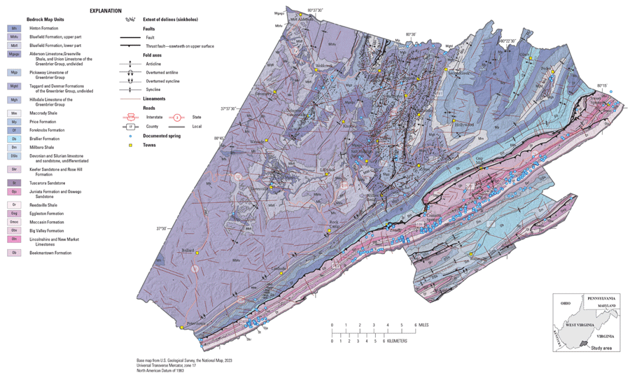
Geologic map of Monroe County from Kozar and others (2023). The full report and an enlarged version of this map are available online at https://doi.org/10.3133/sir20235121.
In addition, a belt of Ordovician-age carbonate rocks with prominent karst development occurs along the northwest flank of Peters Mountain and extends across the entire southeastern border of the county along the state line between West Virginia and Virginia. These Ordovician carbonates were also mapped in more detail in the recent study by Kozar and others (2023) than in Reger and Price (1926). The new mapping used modern stratigraphic nomenclature and divided the Ordovician carbonates into six units including, from oldest to youngest, (1) the Beekmantown Formation, (2) the New Market and Lincolnshire Limestones, undivided, (3) the Big Valley Formation, (4) the Moccasin Formation, (5) the Eggleston Formation, and (6) the Reedsville Shale.
The geologic mapping was enabled by the acquisition of a lidar-derived elevation model for the entire county (Cox and Doctor, 2021a). Using the elevation data, an inventory of karstic closed depressions for the entire county was created, along with a map of the estimated density of dolines and cave entrance locations (Cox and Doctor, 2021a, b, c). The degree of karst development in each of the map units is illustrated on figure 2 as represented by the number of features in each unit.
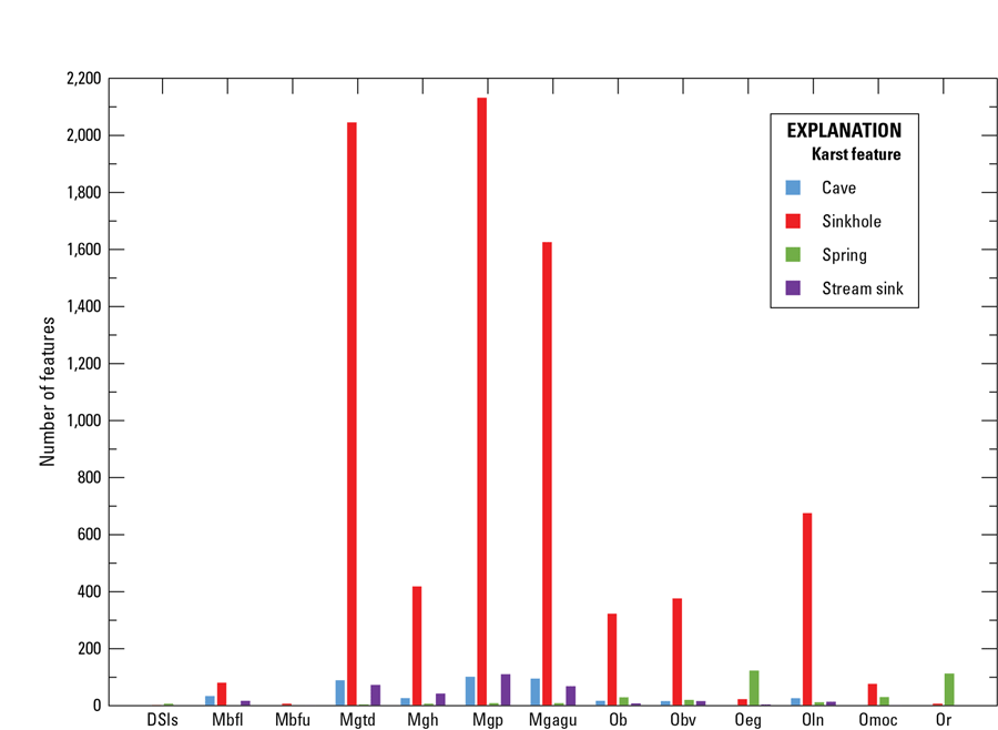
Bar graph of the distribution of caves, sinkholes, springs, and stream sinks by geologic map unit in Monroe County, West Virginia. Abbreviations for the map units are as follows: DSls, Silurian and Devonian limestones and sandstones, undifferentiated; Mbfl, Bluefield Formation, lower; Mbfu, Bluefield Formation, upper; Mgtd, Taggard and Denmar Formations, undivided; Mgh, Hillsdale Limestone; Mgp, Pickaway Limestone; Mgagu, Union Limestone, Greenville Shale, and Alderson Limestone of the Greenbrier Group, undivided; Ob, Beekmantown Formation; Obv, Big Valley Formation; Oeg, Eggleston Formation; Oln, New Market and Lincolnshire Limestones; Omoc, Moccasin Formation; Or, Reedsville Shale (Kozar and others, 2023).
Because of the differences in structural, stratigraphic, and topographic settings, the styles of karst development between the Mississippian and Ordovician rocks are markedly different. Within the Greenbrier Group carbonates, sinkhole development is most evident within low to moderately dipping units of the Pickaway Limestone, Denmar Formation, and Union Limestone. The highest density of closed depressions occurs north of the town of Union in the center of the county (fig. 3).
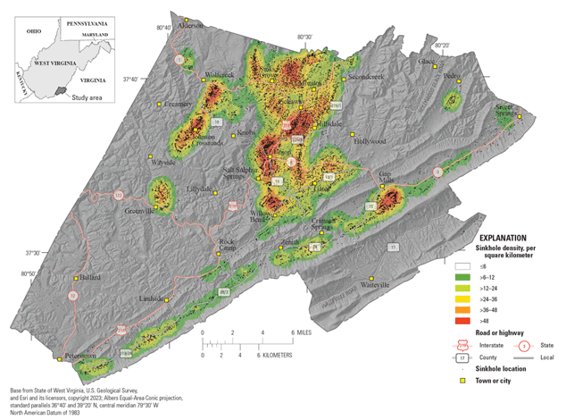
Map showing sinkhole distribution and density in Monroe County, West Virginia (Cox and Doctor 2021a,b,c; Kozar and others, 2023).
The strike of bedding within folds and along faults is largely responsible for controlling regional groundwater movement. For example, within the Mississippian Greenbrier Group in the central portion of the county, two large caves, Union Cave and Hurricane Ridge cave, extend laterally, parallel to newly mapped minor thrust faults. Key to the understanding of karst development in the Greenbrier Group carbonate strata is the recognition of trunk-passage cave development at the contact between the laterally continuous mudstones, limestones, and shales of the Maccrady Formation and the overlying Hillsdale Limestone (Balfour, 2018). A dye trace conducted for the study by Kozar and others (2023) demonstrated surface streamflow sinking at this contact along Taggart Branch south of Gates traveled over 9 miles (14.5 kilometers) to the north across the county and arrived at Dickson Spring 29 days after injection with approximately 8.7 percent dye recovery by mass. The Taggard Formation also contains shale, but it is thin and discontinuous and, therefore, was not found to have a major influence on karst development at its contact with the underlying Denmar Formation, or with the overlying Pickaway Limestone.
Karst development formed within the Ordovician rocks on the northwestern flank of Peters Mountain is geologically and hydrologically distinct from karst development in the Mississippian rocks. The Ordovician karst is similar to a scarp-slope type of karst development in the Greenbrier Group Mississippian rocks on Powell Mountain in southwestern Virginia, first described by Schwartz and Orndorff (2009). Surface streams on the scarp slope of Peters Mountain begin as springs primarily within the Reedsville Shale and the colluvium and ancient alluvial fan deposits of Silurian quartz sandstones that cover the slopes. Epigenetic karstification occurs where these streams sink as they encounter the lithologic contact with older Ordovician limestone units downslope; however, these sinking streams invade a pre-existing paleo-phreatic network. The paleo-phreatic cave passages extend vertically along joints and across bedding within structural folds, then continue along strike and down gradient toward a local base level stream. The deeper phreatic conduit formation may have been influenced by upwelling of warmer water along the St. Clair thrust fault at depth. The presence of deep-seated, long residence time water is evidenced by the spring temperatures and geochemistry. For example, a series of warm springs emerge at Sweet Springs with temperatures up to 23.3 degrees Celsius (Vesper and others, 2019). Additionally, the stable carbon isotope compositions (δ13C) of dissolved inorganic carbon in the thermal spring waters are particularly elevated, in the range of −3 to −5 per mil (Sack and Sharma, 2014; Vesper and others, 2022), indicative of substantial isotopic exchange with the host carbonate bedrock. Associated with these springs are extensive tufa deposits, and the modern springflow continues to precipitate calcium carbonate and some gypsum (Vesper and others, 2019). Moreover, studies of the microbiology from a nearby cave influenced by thermal waters showed evidence of carbonate dissolution occurring as a result of sulfuric acid produced by sulfur-cycling bacterial colonies in the cave (Summers Engel and others, 2001).
The presence of a deep, hypogenic karst flow system within the Ordovician carbonates along the St. Clair thrust zone, as evidenced by warm water sulfidic springs, contrasts with the modern fluviokarst within the Mississippian carbonates of the interior plateau setting of Monroe County. These two karst systems that occur in proximity within the same county warrant additional study to further elucidate the controls on such different styles of karst development.
References Cited
Balfour, W.M., 2018, The contact caves of central Greenbrier County, chap. 11 of White, W.B., ed., Caves and karst of the Greenbrier Valley in West Virginia, in LaMoreaux, J.W., ed., Cave and karst systems of the world: Cham, Switzerland, Springer, p. 207–230. [Also available at https://doi.org/10.1007/978-3-319-65801-8_11.]
Cox, C.L., and Doctor, D.H., 2021a, Lidar-derived imagery and digital elevation model of Monroe County, West Virginia at 3-meter resolution: U.S. Geological Survey data release, https://doi.org/10.5066/P9TKR3XJ.
Cox, C.L., and Doctor, D.H., 2021b, Lidar-derived closed depression vector data and density raster in karst areas of Monroe County, West Virginia: U.S. Geological Survey data release, https://doi.org/10.5066/P9O85K6T.
Cox, C.L., and Doctor, D.H., 2021c, Density raster of caves in Monroe County, West Virginia: U.S. Geological Survey data release, https://doi.org/10.5066/P92JLWRM.
Kozar, M.D., Doctor, D.H., Jones, W.K., Chien, N., Cox, C.E., Orndorff, R.C., Weary, D.J., Weaver, M.R., McAdoo, M.A., and Parker, M., 2023, Hydrogeology, karst, and groundwater availability of Monroe County, West Virginia: U.S. Geological Survey Scientific Investigations Report 2023–5121, 82 p., 3 pls., https://doi.org/10.3133/sir20235121.
Reger, D.B., and Price, P.H., 1926, Mercer, Monroe, and Summers Counties: West Virginia Geological Survey County Geologic Report CGR-15, 963 p., 34 pls., 6 sheets, 1:62,500 scale. [Also available at https://archive.org/details/mercermonroesumm00west/mode/2up.]
Sack, A.L., and Sharma, S., 2014, A multi-isotope approach for understanding sources of water, carbon and sulfur in natural springs of the Central Appalachian region: Environmental Earth Sciences, v. 71, p. 4715–4724. [Also available at https://link.springer.com/article/10.1007/s12665-013-2862-5.]
Schwartz, B., and Orndorff, W., 2009, Hydrogeology of the Mississippian scarp-slope karst system, Powell Mountain, Virginia: Journal of Cave and Karst Studies, v. 71, no. 3, p. 168–179. [Also available online at https://caves.org/wp-content/uploads/Publications/JCKS/v71/cave-71-03-168.pdf.]
Vesper, D.J., Bausher, E.A., and Downey, A., 2022, Comparison of microbial indicators and seasonal temperatures as means for evaluating the vulnerability of water resources from karst and siliciclastic springs: Hydrogeology Journal, v. 30, p. 1219–1232. [Also available at https://doi.org/10.1007/s10040-022-02496-3.]
Vesper, D.J., Moore, J.E., and Edenborn, H.M., 2019, Tufa deposition dynamics in a freshwater karstic stream influenced by warm springs: Aquatic Geochemistry, v. 25, p. 109–135. [Also available at https://link.springer.com/article/10.1007/s10498-019-09356-9.]
White, W.B., ed., 2018, Caves and karst of the Greenbrier Valley in West Virginia, in LaMoreaux, J.W., ed., Cave and karst systems of the world: Cham, Switzerland, Springer, 411 p. [Also available at https://doi.org/10.1007/978-3-319-65801-8.]
A Karst-Rich Impact Crater: Drill Cores From the Flynn Creek Crater, North-Central Tennessee
Abstract
Flynn Creek crater is considered the birthplace of impact speleology, a term coined by Milam and Deane (2006) to describe the study of caves within impact craters. Flynn Creek crater was formed in a shallow sea environment approximately 360 million years ago and is currently the only known impact structure to host a cave within its central uplift. This unique and scientifically rich location was the focus of a multiyear drilling program that occurred from the late 1960s to the late 1970s and resulted in the collection of over 3,000 meters of continuous drill core acquired from this impact crater. These samples are now part of the U.S. Geological Survey (USGS) Astrogeology Science Center (ASC) Terrestrial Analog Sample Collections (TASC) and are available to the science community for research and teaching purposes. Available online at: https://www.usgs.gov/centers/astrogeology-science-center/science/terrestrial-analog-sample-collections.
Introduction
Flynn Creek crater is a 360-million-year-old impact crater situated in the Highland Rim physiographic providence of present day north-central Tennessee (N 36°17', W 85°40') (Roddy, 1968). The crater is about 3.8 kilometers in diameter, more than 200 meters (m) deep, has a flat floor, terraced rim, and a central uplift (Roddy, 1977a, b; Wilson and Roddy, 1990; Evenick, 2006). Flynn Creek crater is one of the original six structures on Earth to be confirmed as having an impact origin (the others being Meteor Crater, Arizona, United States; Reis Crater, Germany; Waba, Australia; Hollifard, Canada; and Bosumtwi, Ghana), as well as the first impact crater recognized to have formed in a marine environment (Jaret and King, 2018).
At the time of impact, this area of Tennessee was part of a shallow Late Devonian sea, underlain by Ordovician-age carbonates (Roddy, 1977a; Klapper, 1997; Tucker and others, 1998; Schieber and Over, 2005). When the impactor struck, marine sediment was excavated from the rapidly forming transient crater and deposited as ejecta. Following this initial displacement of sediment was the movement and volumetric rebound of rock beneath the crater floor (Ulrich and others, 1977), causing deep-seated rocks to be violently forced upward, resulting in a central peak inside the crater (Melosh, 1982). Post-impact erosion and deposition on the original transient crater floor were soon inundated by coarse breccias, grading into finer-grained breccias (Roddy, 1977b). Eventually, the Late Devonian sea breached the crater’s rim, leading to marine resurgence and the deposition of black, silty muds that later lithified into the Chattanooga Shale (Roddy, 1968, 1979, 1980).
Karst Features in an Impact Crater
Flynn Creek crater contains the highest concentration of known karst features in Jackson County, Tennessee, and is the only known impact crater in the world to host a cave in its central uplift (Milam and others, 2005). Currently, 12 caves have been identified: 9 are located along or near the crater rim, 1 within the central uplift, and the remaining 2 do not appear to be influenced by the structure of the crater (Milam and others, 2006).
Cave climate is typically buffered from the outside environment, enabling diverse flora and fauna to thrive (Milam and Deane, 2006). Equivalent environments on other planetary bodies may also provide some protection from the harsh outside elements, meaning karst features within impact craters could prove extremely valuable when searching for life on other planets (Milam and Deane, 2006). Flynn Creek crater can, therefore, be used as a resource for learning how to detect caves in impact craters on other planetary bodies, as well as improve our understanding of the structural controls inflicted by impact-related morphologies on caves (Milam and Deane, 2006; Cushing and others, 2007).
Impact Origin Versus Volcanic Origin
An impact origin had not always been the accepted view behind the formation of Flynn Creek crater. In the 1920s, Lusk (1927) noted that the expansive and relatively uniform Chattanooga Shale (thicknesses of 3–15 m) unexpectedly increased up to 46 m in thickness in the Flynn Creek area. The presence of karst across this region led Lusk to conclude that this structure was the result of a collapsed near-surface cave, forming a sinkhole that later filled in with younger-aged sediments like the Chattanooga Shale (Hagerty and others, 2013). Roughly a decade later, Wilson and Born (1936) determined the area to be riddled with faults and deformation, including large blocks situated about 150 m higher than their expected original location, concluding that a cryptovolcanic explosion was responsible (Roddy, 1964; Hagerty and others, 2013). In the same year, Boon and Albritton (1936) found that structural features typically attributed to cryptovolcanic explosions (for example, strata dipping away from the crater’s center, concentric faulting) were almost identical to features associated with a meteorite origin. It was not until shatter cones (conical-shaped rocks with a striated and fractured surface, known only to form from a meteorite impact) were discovered at Flynn Creek crater that an impact origin was fully accepted (Dietz, 1960; Roddy, 1968).
Structural Deformation
Within the last 100 years, impact cratering studies have made leaps and bounds in our understanding of not only the surface evolution of our Moon and other planetary bodies, but also how meteorite impacts have influenced Earth’s geologic history (French, 1998). Depending on the size of the impactor and resulting transient crater, different degrees of modification influence the final shape of a crater (Melosh, 1989). The smallest impact craters are in the form of a simple bowl shape (fig. 1A). As crater size increases and a crater’s morphology becomes more complex, terraced rims and a central uplifted peak form (fig. 1B). Increasing in complexity from there, peak ring structures are formed when the original uplifted peak collapses due to overextension, resulting in an interior ring on the floor of a crater (fig. 1C), followed by large impact basins with multiple rings (fig. 1D). Most complex of all are massive flat-floored basins, such as the South Pole-Aitken basin (2,500 kilometers in diameter) on the Moon (Baldwin, 1974; Gault and others, 1975; Pike, 1976; Roddy, 1979; Melosh, 1989; French, 1998).
Increases in structural deformation occur in conjunction with morphological complexities. Characterizing the extent and influence of deformation associated with an impact crater and the resultant morphology are important factors in understanding the evolution of a planet’s surface (Roddy, 1979). The ability to carry out such work on a planetary body beyond Earth is very limited, restricted mostly to satellite or orbiter imagery and only studying what is exposed on the surface. Terrestrial impact craters are incredibly valuable to the development of our understanding of impact-related processes. Having direct access to structurally deformed rocks that experienced the intense heat and pressure that only an impact could generate gives us the ability to characterize the different stages of impact crater morphologies on Earth and then extrapolate that to other planetary bodies (Roddy, 1979).
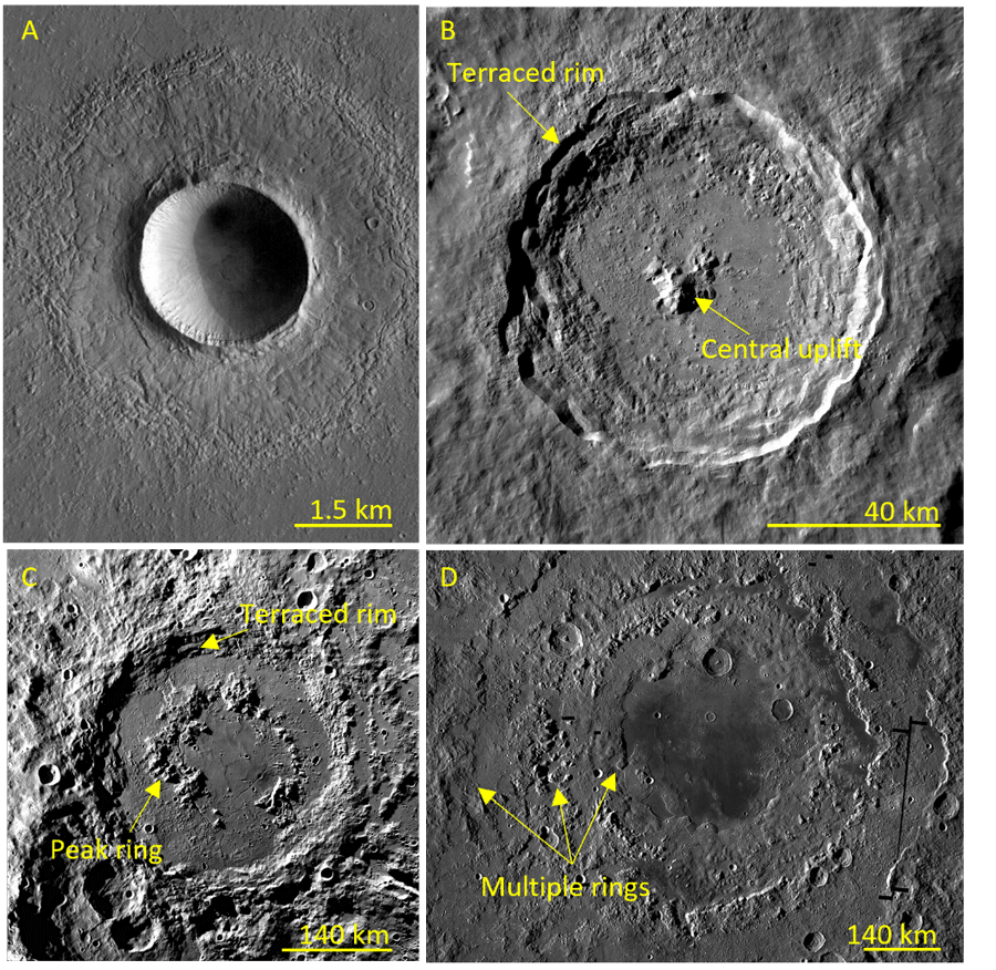
Increasingly complex impact crater morphologies. Note the difference in scale between the images. A, Simple bowl-shaped crater. Image credit: Mars Global Surveyor image PIA02084; B, Tycho crater, a flat-floored crater with terraced rims and a central uplift. Image credit: NASA, Lunar Reconnaissance Orbiter (LRO); C, Schrödinger, a peak ring basin. Image credit: NASA LRO; D, Orientale, a multi-ringed basin. Image credit: NASA LRO.
Flynn Creek Crater Drilling and Preliminary Findings
Detailing the extent of brecciation, depth of deformation, and the level of shock metamorphism for complex craters can be achieved through studying terrestrial impact craters. Dr. David Roddy (U.S. Geological Survey [USGS]) sought to acquire such information at Flynn Creek crater through a multi-year drilling program (Roddy, 1977a, b; 1979). Drilling was carried out in two phases: phase I occurred in 1968 and resulted in six drill holes and about 760 m of continuous core; phase II occurred in 1978–1979, resulting in an additional 12 drill holes and about 3,060 m of continuous core (fig. 2; Roddy, 1980).
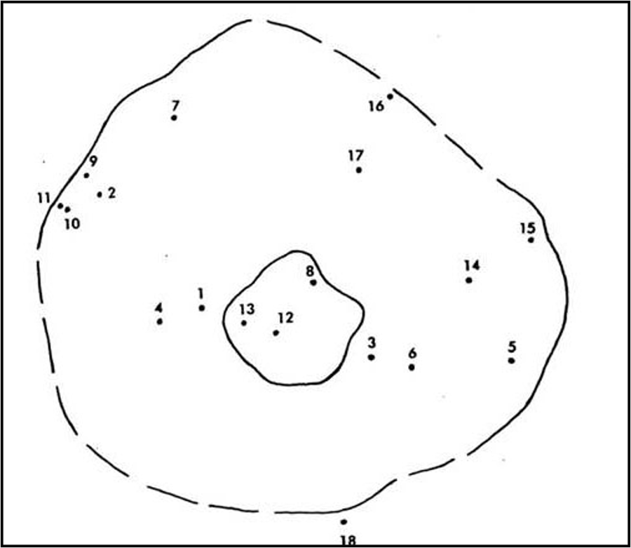
Sketch of approximate locations of drill holes at Flynn Creek crater (from Roddy, 1980).
Evaluating the cores collected from the drilling program led Roddy (1968, 1977a, 1980) to further determine that Flynn Creek crater has an average depth of about 90 m below the pre-impact surface, its breccia lens is only about 40 m thick, and at a depth of about 100 m below the breccia lens, deformation is no longer visible. These findings infer that the impactor penetrated and excavated a wide, yet very shallow crater (fig. 3; Roddy, 1968, 1977a, b; 1980). Cores drilled into the central uplifted peak and on its flanks showed deep-seated target rocks were excavated from a depth of about 450 m, and brecciated rocks were observed down to a depth of about 770 m, which shallowed to about 450 m near the edges of the uplift (Roddy, 1977b, 1980).
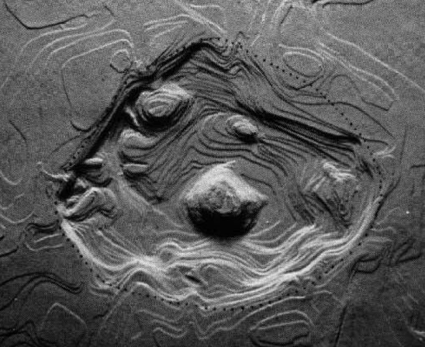
Shaded-relief reconstruction of the topography of Flynn Creek crater immediately after impact, prior to deposition of the overlying Chattanooga Shale (from Roddy, 1979).
Curation and Preservation of the Flynn Creek Crater Cores
Over 2,000 core boxes from Dr. David Roddy’s drilling program were shipped to Flagstaff, Arizona, where it was intended to make the collection available for public access (Hagerty and others, 2013). Unfortunately, such plans were halted when Dr. Roddy passed away unexpectedly in 2002. A decade later, a core recovery and preservation effort was implemented by Dr. Justin Hagerty (USGS). This resulted in transporting the core boxes to large secure shipping containers (fig. 4) located at the USGS Flagstaff Science Campus, and the recovery and preservation of damaged core boxes were carried out alongside a detailed inventory process, in which information on each core box was recorded in a digital database (Hagerty and others, 2013; Gaither and others, 2015, 2017, 2021).
USGS ASC Flynn Creek Crater Sample Collection
This collection, as well as other sample collections are housed by the USGS Astrogeology Science Center (ASC) Terrestrial Analog Sample Collections (TASC) program (Gaither and others, 2015, 2021). The TASC provides the scientific community with a range of samples, including but not limited to, impact crater drill cores and cuttings, hand samples, and rock powders, all of which are available for use in scientific research.
Available on the USGS ASC Flynn Creek Crater Sample Collection website are high-resolution images of each cataloged drill core within the core library (fig. 5). Each core box can be evaluated virtually on the website, and samples of interest can be requested by emailing the author (agullikson@usgs.gov). Instructions on obtaining data from the Flynn Creek crater and other sites are currently available from the website (U.S. Geological Survey, 2024).
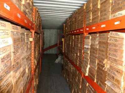
Flynn Creek crater core boxes stored in large shipping containers. Photograph taken by Justin Hagerty, U.S. Geological Survey.
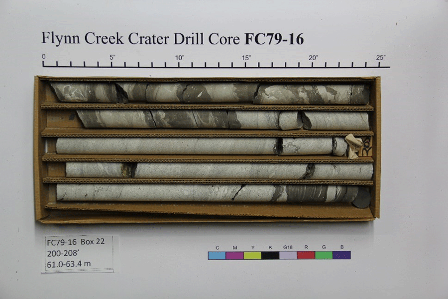
Example of drill core box from the Flynn Creek Crater Sample Collection. FC79-16 refers to the year drilling took place, followed by the drill core number. Lower left of image shows sample depth in both feet and meters (Photograph from U.S. Geological Survey, 2024).
Use of the Collection
Recent work utilizing the Flynn Creek Crater Sample Collection has resolved further questions around the modification stage of a marine-based impact structure. The shape of Flynn Creek crater has recently been described as an “inverted sombrero,” resulting from a high degree of erosion caused by marine resurgence into the weakened target material (Adrian and others, 2019). Drill cores from the flanks of the central uplift (FC77-1) and the (colloquial) “moat,” that is, the low-lying area surrounding the central uplift (FC77-3 and FC67-3), were used to delineate changes in the depositional environment of the breccia layer (slump deposits into a subaqueous setting, deposition from suspension) (Adrian and others, 2017; De Marchi and others, 2019). Cryptocrystalline melt clasts have also been recently discovered in some of the drill cores (Adrian and others, 2017).
Most recently, hydrocode modeling, in conjunction with drill core studies, has begun to refine the approximate sea depth when the impact occurred (Bray and others, 2022). Sea depth plays an important role in constraining peak shock pressures and the mechanisms behind the formation of a central uplift in a marine setting, and therefore can be used to calculate an estimated depth for the highest shocked material beneath the central uplift and crater floor (Bray and others, 2022). Hydrocode simulations by Bray and others (2022) also indicate that highly shocked material within Flynn Creek crater may be at greater depths than previously expected, buried beneath more than 200 m of minimally shocked material.
ASC TASC Upcoming Work
Over the next year, a detailed digital database is planned to be released that provides information for each drill core box, including drill hole number, box number, start and end depth (in feet and meters), geologic unit(s), lithologic descriptions, and keywords used to facilitate discoverability among samples. This database and accompanying drill core images will be publicly available as a USGS data publication. Additionally, samples will be registered with both ReSciColl (Registry of Scientific Collections), formerly known as the National Digital Catalog, and SESAR2 (System for Earth and Extraterrestrial Sample Registration). Both programs provide an infrastructure aimed on preserving data in a digital format, including detailed metadata records and web-based applications that are used to increase user accessibility. One added benefit to using SESAR2 services is that each sample registered is assigned an IGSN (International Generic Sample Number) with a SESAR2 pre-fix and suffix, upholding the FAIR (Findability, Accessibility, Interoperability, and Reuse) guiding principles for scientific data management (Wilkinson and others, 2016). Each sample, therefore, has a globally unique identifier that enables easy tracking (for example, related samples, parent and (or) child) and publication searches. Both registries allow for batch registration methods, minimizing the redundancy of the uploading process but expanding the digital footprint to bring awareness of the sample collection to a broad range of scientific communities.
Summary
The USGS ASC Terrestrial Analog Sample Collections currently house three individual collections: Flynn Creek Crater, Meteor Crater, and the Shoemaker Collection. These collections preserve the scientific legacies of pioneer planetary scientists, Dr. Eugene Shoemaker and Dr. David Roddy, and are available to the scientific community for research and teaching purposes.
The Flynn Creek Crater Sample Collection houses over 2,000 boxes of cores from 18 separate boreholes within the impact crater. All cores in this collection have been imaged. In the coming months, the Flynn Creek Crater Sample Collection digital database will be published and registered with both ReSciColl and SESAR2 to increase discoverability. If interested in conducting research using these samples, please see U.S. Geological Survey (2024).
Acknowledgments
The curation and preservation of this collection has been supported by the National Aeronautics and Space Administration (NASA) through the Planetary Geology and Geophysics program via grant NNH14AY73I, and by an interagency agreement between the U.S. Geological Survey ASC and the NASA Science Mission Directorate. The authors would like to thank Sonya Bogle and Marc Hunter for their helpful comments that have improved the clarity of this manuscript.
References Cited
Gaither, T.A., Hagerty, J.J., and Bailen, M., 2015, The USGS Flynn Creek crater drill core collection—progress on a web-based portal and online database for the planetary science community [abs.]: Proceedings of the 46th Lunar and Planetary Science Conference, The Woodlands, Texas, March 16–20, 2015, abstract #2089.
Gaither, T.A., Hagerty, J.J., Villareal, K.A., Gullikson, A.L., and Leonard, H., 2017, Flynn Creek impact crater—petrographic and SEM analyses of drill cores from the central uplift [abs.]: Proceedings of the 48th Lunar and Planetary Science Conference, The Woodlands, Texas, March 20–24, 2017, abstract #2263.
Jaret, S.J., and King, D.T., Jr., 2018, Revisiting the Flynn Creek impact structure, Jackson County, Tennessee, in Engel, A.S., and Hatcher, R.D., Jr., eds., Geology at every scale—field excursions for the 2018 GSA Southeastern Section meeting in Knoxville, Tennessee: Geological Society of America Field Guide 50, p. 75–79.
Klapper, G., 1997, Graphic correlation of Frasnian (Upper Devonian) sequences in Montagne Noire, France, and western Canada, in Klapper, G., Murphy, M.A., Talent, J.A., eds., Paleozoic sequence stratigraphy, biostratigraphy, and biogeography—studies in honor of J. Granville (“Jess”) Johnson: Boulder, Colorado, Geological Society of America Special Paper 321, p. 113–184.
Melosh, H.J., 1982, A schematic model of crater modification by gravity: Journal of Geophysical Research, v. 87, issue B1, p. 371–380. [Also available online at https://agupubs.onlinelibrary.wiley.com/doi/abs/10.1029/JB087iB01p00371.]
Milam, K.A., Deane, B., and Oeser, K., 2005, Caves of the Flynn Creek impact structure, in Milam, K.A., Evenick, J., and Deane, B., eds, Field guide to the Middlesboro and Flynn Creek impact structures—Impact Field Studies Group: 69th Annual Meteoritical Society meeting, Gatlinburg, Tennessee, p. 36–45.
Ulrich, G.W., Roddy, D.J., and Simmons, G., 1977, Numerical simulations of a 20-ton TNT detonation on the earth’s surface and implications concerning the mechanics of central uplift formation, in Roddy, D.J., Pepin, R.O., and Merrill, R.B., eds., Impact and explosion cratering: New York, Pergamon Press, p. 959–982.
U.S. Geological Survey, 2024, Terrestrial Analog Sample Collections: Website accessed October 10, 2024, at https://www.usgs.gov/centers/astrogeology-science-center/science/terrestrial-analog-sample-collections.
High-Resolution, Three-Dimensional Groundwater Flow Mapping in the Great Onyx Groundwater Basin, Mammoth Cave National Park, Kentucky
Abstract
Understanding spatial distributions and temporal variability of groundwater flow and chemistry in karst aquifers is a complex task using fluorescent dye tracing, exploration and mapping of cave streams, geology and potentiometric surface mapping, and other methods. In the 1970s and 1980s, Jim Quinlan and colleagues completed hundreds of dye traces in and around Mammoth Cave National Park and mapped more than 75 kilometers of cave passages including many cave streams. A classic 1981 map defined the major karst drainage basins. Updated in 1989 (Quinlan and Ray, 1989), these and subsequent data are now archived by the Kentucky Geological Survey as the Karst Atlas of Kentucky: Karst Groundwater Basin Maps (Kentucky Geological Survey, 2024).
Great Onyx (GO) Spring in the Park’s Hilly Country was shown but not labeled in the Karst Atlas, and little was known until early 2000s dye traces by Joe Meiman led to the first basin map of about 4 square kilometers (Kentucky Geological Survey, 2024). A high-resolution groundwater flow investigation was started in 2017 to better define the GO basin boundaries and the aquifer’s three-dimensional (3D) internal plumbing. This represents the next generation of fine-scale karst groundwater flow characterization, supporting design of a long-term monitoring system to quantify carbon, nutrient, and sediment fate and transport. Remarkable access to the basin’s essentially pristine contemporary underground flow system is made through more than 20 kilometers of cave passages in GO and Mammoth Caves. The two caves have been hydrologically connected, and dye tracing has shown that GO Spring is fed by at least a third-order stream. A model was also developed to explain an evolutionary decoupling of surface topography and groundwater flow in the ravines of the Hilly Country (Kentucky Geological Survey, 2024).
References Cited
Kentucky Geological Survey, 2024, Karst Atlas of Kentucky—Karst Groundwater Basin Maps: Website accessed October 10, 2024, at https://www.uky.edu/KGS/water/research/kaatlas.htm.
Planned Alternative Water Supply Technologies Utilizing the Karst Aquifers of Texas
Abstract
Alternative water supply technologies include aquifer storage and recovery, and brackish groundwater desalination. Aquifer storage and recovery extends the duration water supplies are available by storing them underground for later retrieval. Most desalination projects in Texas use reverse osmosis membranes to remove minerals and contaminants from brackish water to create less saline water supplies. In addition to traditional groundwater production wells, these alternative water supply technologies may also rely on aquifers. Aquifer storage and recovery projects use aquifers as storage zones for recoverable water and may also use groundwater as a source of water to inject and store. Some desalination facilities use aquifers as a source of brackish water and may also use deep, confined saline aquifers as storage zones for concentrate disposal.
Of Texas’ 31 major and minor aquifers, 11 contain karstic zones. The most widespread karst aquifers in Texas are the Cretaceous Edwards and Trinity aquifers. Four of the 5 existing aquifer storage and recovery projects and 8 of the 39 existing brackish groundwater facilities in Texas utilize these aquifers (fig. 1). Other karst and limestone aquifers utilized by existing alternative water supply facilities include the Bone Spring–Victorio Peak aquifer, which provides brackish groundwater for desalination and an unconfined storage zone for recharge via infiltration, and the Fusselman and Montoya Formations, which are used to dispose of desalination concentrate.
The Texas State Water Plan is updated on a 5-year cycle to provide a water supply road map. During this update cycle (2023–2027), the plan compares projected water demands with projected water supplies to estimate needs for five decades into the future. Mostly driven by population growth along the Interstate 35 corridor, projected growing water demands in this region are leading to more planned water supply strategies involving the underlying Edwards and Trinity aquifers. In addition to new traditional groundwater production projects, communities and water suppliers plan to use alternative water supply technologies to meet anticipated needs. In the 2022 State Water Plan (Texas Water Development Board, 2022), alternative water supply projects that would utilize karst aquifers in Texas include 14 of 34 recommended aquifer storage and recovery projects and 5 of the 33 recommended brackish groundwater desalination projects (fig. 1).
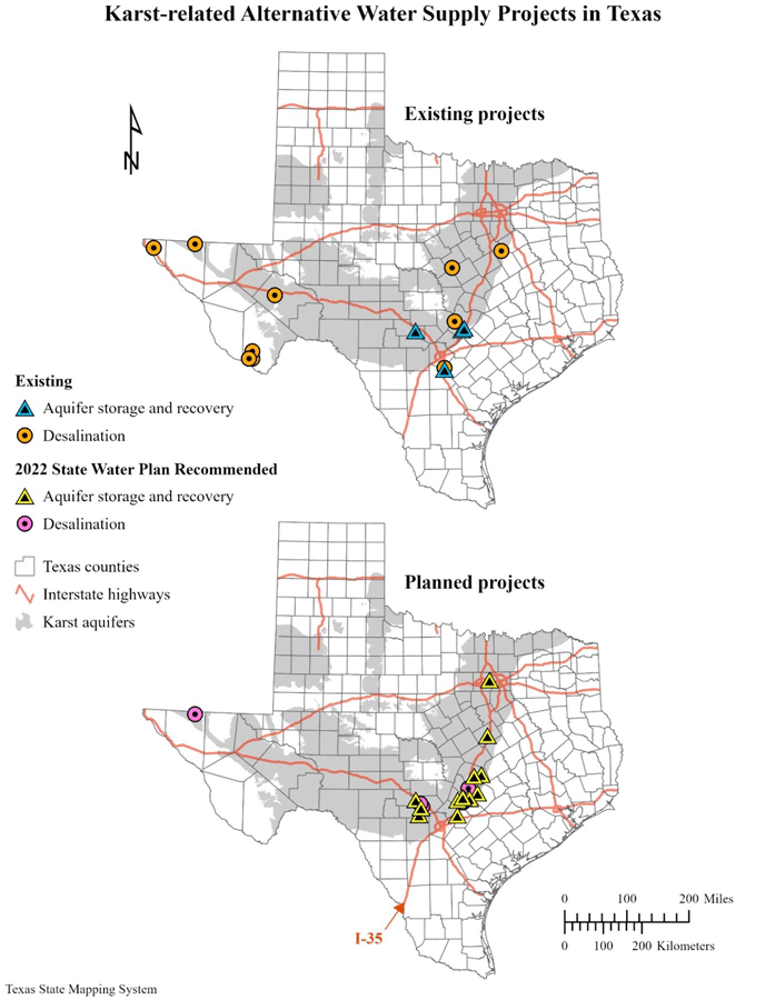
Maps showing the existing and planned alternative water supply projects in Texas that will utilize karst aquifers (Texas Water Development Board, 2022).
To support these planned alternative water supply projects, the benefits and challenges identified during the development and operation of existing alternative water supply projects in the karst aquifers of Texas have been reviewed. These topics include rapidly responsive water table changes in the high transmissivity portions of the aquifers, fast water velocities related to steep hydraulic gradients, large groundwater production volumes supported by voids and fractures, geochemical complexities from high mineral content and water mixing, and habitat conservation for groundwater species.
Reference Cited
Texas Water Development Board, 2022, Water for Texas, 2022 State Water Plan: Austin, Texas, 202 p., https://www.twdb.texas.gov/waterplanning/swp/index.asp.
The Underwater Karst System of Mount Gambier, South Australia: A Little Tapped Archive of Late Quaternary Environmental Change
Abstract
The Eocene- to Miocene-age Gambier Limestone in the Gambier Basin, situated in the southeast corner of the state of South Australia, hosts more than 50 recorded caves and cenotes (Webb and others, 2010). Most of these caves and sinkholes extend below the water table, providing some of the best cave diving opportunities in the world as well as significant opportunities for studying palaeoenvironmental archives. The most extensive underwater cave system recorded in the region, with more than 10 kilometers of surveyed passages, is the Green Waterhole-Tank Cave Complex; a connection between these two caves was established in 2018. This system largely sits under land owned by the Cave Divers Association of Australia (CDAA) and is a South Australian State Heritage Listed site nominated for its outstanding values in palaeontology, speleology, and geology. Access to the Green Waterhole-Tank Cave Complex is an Advanced Cave rated site and is accessible only through the CDAA with access points on CDAA and Department of Environment and Water (DEW) managed properties. The correct level of training and restricted access to the site is imperative to ensure safety of the divers and protection of the cave.
Despite divers exploring the Gambier Limestone caves since the 1950s, and the known potential of karst systems to preserve rich environmental records, underwater cave deposits in this region have remained relatively untapped as sources of palaeoenvironmental information. This is due to the challenges associated with safe scientific diving in underwater caves and the limited number of scientifically trained cave divers (with less than six active scientific advanced cave divers in Australia). In the Gambier Limestone, palaeoenvironmental archives previously recovered from underwater caves consisted of late Quaternary vertebrate fossils and associated sediments, and freshwater stromatolites (Newton, 1988; Kelly, 1998; Mather and others, 2024). Additional palaeoenvironmental samples that were collected between 2022 and 2024, as well as the diving considerations associated with their collection and documentation, are described herein.
Although samples have been collected from Gouldens Hole, Engelbrecht Cave East, and Green Waterhole (also known as Fossil Cave), all in the Mount Gambier region, the focus of the most recent investigations has been in a chamber of the Green Waterhole-Tank Cave Complex called the Bone Room. Primary access is through the Tank Cave entrance; this requires an approximately 45-minute, 950-meter swim before accessing the chamber through a series of tight constrictions. Alternative access can be achieved through Green Waterhole, and although this presents a shorter access, the extreme constriction between Green Waterhole and Tank Cave makes this route more difficult and hazardous. In our fieldwork the Tank Cave entry was used, with the Fossil Cave passages considered a strategic access point to be used only in emergencies. The length of access to the Bone Room required us to critically evaluate the following diving considerations: (1) open circuit versus closed circuit rebreathers; (2) number and positions of stage tanks; (3) mitigation of decompression through the use of Nitrox; (4) level of training and experience of the cave divers; (5) the number of divers in the system at any one time; and (6) the number of dives per day impacting ‘silt-out’ (sediment settling time required for visibility), due to the cave system having no significant flow.
By virtue of their underwater setting and difficult access, palaeoenvironmental deposits within these phreatic caves remain largely pristine and undisturbed (Louys, 2018). We have been able to recover the following palaeoenvironmental archives from underwater settings: (1) micro and macro vertebrate fossils including extinct megafauna; (2) historical bone deposits associated with the earliest European colonization of the region; (3) samples associated with palaeontological and zooarchaeological remains for dating, including samples for optically stimulated luminescence and electron spin resonance dating; (4) sediment cores for pollen analysis; (5) environmental and ancient DNA samples from water and sediment; (6) speleothem deposits, particularly calcite rafts; and (7) freshwater stromatolite deposits. Although analysis of these samples is still ongoing, this project demonstrates the significant scientific value of a wide range of environmental archives and proxies hosted in underwater cave deposits and highlights ways that these can be successfully extracted and examined. This project is ongoing, and methods and techniques are still being refined in collaboration with the CDAA, scientific divers, and associated researchers.
References Cited
Mather, E.K., Lee, M.S., Fusco, D.A., Hellstrom, J., and Worthy, T.H., 2024, Pleistocene raptors from cave deposits of South Australia, with a description of a new species of Dynatoaetus (Accipitridae: Aves)—morphology, systematics and palaeoecological implications: Alcheringa, An Australasian Journal of Palaeontology, v. 48, no. 1, p. 134–167.
Mineral-Attached Microbial Communities in Karstic Caves of North Central Florida
Abstract
The Upper Floridan Aquifer (UFA), one of the world’s most productive freshwater aquifers, is largely made up of Eocene- to Oligocene-age carbonate rocks that comprise the Suwannee and Ocala Limestones (Williams and Kuniansky, 2016). Though the Ocala Limestone consists almost entirely of pure carbonate rock, the Suwannee Limestone may contain quartz sand and impurities. Overlying the Suwannee and Ocala Limestones and Avon Park Formation is the Miocene-age Hawthorn Group. This group consists predominantly of siliciclastic clays and sands with basal limestone deposits, some dolomite, and large deposits of phosphate minerals (Scott, 1990; Williams and Kuniansky, 2016).
The UFA’s karst topography facilitates dynamic water-rock interactions, allowing for the formation of biofilms that serve as localized hotspots for biological activity intimately connected to rock and mineral surfaces (Jones and Bennett, 2014; Casar and others, 2021). Prior work in the UFA has characterized the groundwater microbial communities, revealing diverse microbial life discharging from the aquifer despite low cell biomass (Malki and others, 2020; Scharping and Garey, 2021; Qi and others, 2023; Barry-Sosa and others, 2024). In aquifer environments, microbial biomass is estimated to be dominated by communities attached to surfaces (Flemming and Wuertz, 2019). However, these communities have rarely been characterized in detail. Furthermore, the contribution of rocks and mineral-associated microbial communities to the overall microbial diversity of aquifer caves and conduits remains poorly understood.
In this study, eight diver-accessible water-filled caves of springs in north and north-central Florida were used to investigate the microbial communities in the subsurface. Sampling locations chosen for this work consisted of both first (more than or equal to 2.83 cubic meters per second [m3/s]) and second (0.28–2.83 m3/s) magnitude springs, with each spring connected to extensive cave networks. Most locations are situated in the unconfined portion of the aquifer, providing access to rocks and minerals of the Suwannee and Ocala Limestones. Two sites are within the semi-confined aquifer and provide access to rocks and minerals of the Hawthorn Group.
Utilizing scanning electron microscopy and electron dispersive spectroscopy (SEM-EDX), microbial biofilms on sediment grains, carbonate, and iron-oxyhydroxide minerals were documented. Micrographs showed diverse biofilm architectures across all samples. Biofilms from carbonate cave walls showed homogenous structures of helical stalks whereas micrographs from silica quartz sands showed clustered biofilms with eukaryotic diatoms encased in calcium deposits and biogenic silica. Iron-rich clays revealed sparse extracellular polymeric substance (EPS) and little biofilm formation.
These results show that microbial biofilms are present at macro and microscopic scales and provide visual evidence of diverse microbial biofilms in association with various mineral substrates. Future studies will expand on this SEM characterization as well as explore chemoautotrophy in biofilm communities to elucidate subsurface contributions to carbon cycling in the aquifer, providing a holistic view of groundwater ecosystem processes occurring in the UFA.
References Cited
Barry-Sosa, A., Flint, M.K., Ellena, J.C., Martin, J.B., and Christner, B.C., 2024, Effects of surface water interactions with karst groundwater on microbial biomass, metabolism, and production: EGUsphere, p. 1–35, https://doi.org/10.5194/egusphere-2024-49.
Flemming, H.C., and Wuertz, S., 2019, Bacteria and archaea on Earth and their abundance in biofilms: Nature Reviews Microbiology, v. 17, no. 4, p. 247–260, https://doi.org/10.1038/s41579-019-0158-9.
Williams, L.J., and Kuniansky, E.L., 2016, Revised hydrogeologic framework of the Floridan aquifer system in Florida and parts of Georgia, Alabama, and South Carolina: U.S. Geological Survey Professional Paper 1807, 140 p., 23 pls., http://dx.doi.org/10.3133/pp1807.
Disappeared Blind Valleys and Phantom Channels on Recent Digital U.S. Geological Survey 7.5-Minute Minnesota Topographic Maps
Abstract
Blind valleys are recognized features in karst terranes (for example, Jennings, 1985, p. 95–99, and Ford and Williams, 2007, p. 359–361). In the downstream direction, blind valleys typically end at an abrupt bedrock headwall. The surface stream sinks at one or more stream sinks, swallets, or sinkholes at the base of the headwall. Perennial or intermittent surface streamflow simply ends at the sink points. A blind valley is a closed basin and if deeper than the contour interval of the map, is shown as closed contour lines with hachures. Because they divert surface runoff into active groundwater flow systems, blind valleys are critical features in understanding the integrated surface-subsurface character of karst terranes. Blind valleys introduce surface water directly into rapid groundwater flow systems.
Four blind valleys are shown correctly on the 1960s paper versions of the Cherry Grove, Minnesota-Iowa, and Wykoff, Minnesota 7.5-minute U.S. Geological Survey (USGS) topographic maps. Decades of field observations, multiple groundwater traces using fluorescent dyes, and recent lidar-derived elevation mapping have documented their existence unambiguously and in detail. However, these blind valleys have “disappeared” from the recent (2013, 2016, and 2019) digital versions of the Cherry Grove and Wykoff topographic maps.
On the 1967 Cherry Grove map, the perennial upper Canfield Creek sinks in the York Blind Valley in section 21 of York Township. Repeated groundwater traces (MGTD, 2024) show that the water sinking in the York Blind Valley resurges in Odessa Spring on the Upper Iowa River about 11 miles east-southeast of the York Blind Valley. The York Blind Valley not only pirates 8.9 square miles of the Root River basin to the Upper Iowa River basin, but the York Blind Valley creates an interstate water transfer of surface water from Minnesota to Iowa.
On the Cherry Grove map, the perennial upper Canfield Creek is shown correctly as a continuous blue-line feature entering the York Blind Valley and flowing across the blind valley until the stream sinks in the terminal swallet; the blue line ends at the terminal sinking point. The York Blind Valley is shown as closed, hachured 1290- and 1300-foot contour lines. From the end of the blind valley for approximately 3,000 feet southeast downstream, in a surface swale, no blue line indicative of streamflow is shown; intermittent surface flow is then shown as a dashed blue line.
On the recent digital versions of the Cherry Grove map, the York Blind Valley is not shown as closed, hachured contour lines. A “phantom” (non-existent) straight channel is shown connecting the 1290- and 1300-foot contour lines around the blind valley, with those contour lines farther down the valley. Canfield Creek is shown (incorrectly) flowing through the blind valley, and the phantom channel is shown as a dashed blue line, indicating intermittent streamflow. The analogous modifications are true for three other blind valleys on the Cherry Grove and Wykoff topographic maps. Surface streams that are not present are now shown as blue-line features through and downstream from the blind valleys, while hachures that once indicated the blind valleys are now gone.
These are not accidental changes or based on updated information. The USGS National Geospatial Program has confirmed that it was an “automated cartographic process issue” (Mitch Bergeson, National Map Liaison—IA, MN, WI, written commun., 2023) and that errors reside in the current USGS National Hydrography Dataset (NHD) (Joel Skalet, National Geospatial Technical Operations Center, written commun., 2023). All these changes are contradicted by lidar data and field observations.
These four examples raise a fundamental question: Do analogous, incorrect changes exist on other recent digital versions of USGS topographic maps available online in karst areas around the United States? Such errors would present potentially serious environmental management problems. Environmental management decisions typically are based on “the most recent available maps and information” from authoritative sources such as the USGS. The individuals and agencies making such decisions may be unaware of the existence of karst features in their areas that are correctly shown on the 1960s maps. Management decisions based on incorrect information on the digital topographic maps could have major, unintended consequences.
References Cited
MGTD, Minnesota Groundwater Tracing Database, 2024, Minnesota Department of Natural Resources, https://www.dnr.state.mn.us/waters/groundwater_section/mapping/springs-gtd.html.
Springs of Virginia: A Hydrogeologic Analysis of a Recently Assembled Database of Virginia Springs
Abstract
All historical and modern spring data available to or collected by the author were compiled into a single database that was used to document the ranges of physical and chemical spring characteristics throughout Virginia, and for the first time, investigate geologic factors that may influence their occurrence in the region (Maynard, 2023a, b). The spring database was examined based on (1) the geologic unit from which the springs discharged; (2) proximity to major fault systems, geologic contacts, dikes, and fold axes; and (3) distribution across a major river basin. Data were processed from a variety of sources to remove duplication, improve locational accuracy, and evaluate available water quality sampling results. The current database includes 1,638 spring locations, 5,913 unique field measurement events, and 2,916 laboratory water quality sampling events (Maynard, 2023b). Coverage spans all five physiographic provinces, but the bulk of field and sampling results are currently in the State’s northern Valley and Ridge province. Spring locations were improved when possible, through fieldwork and the use of high-resolution orthoimagery and LiDAR (Light Detection and Ranging) data. Sampling and laboratory analysis errors were evaluated for a subset of springs by calculating anion and (or) cation charge balance values when possible.
The largest geochemical differences occurred between springs in different rock type groups. Springs in igneous and metamorphic rock areas of the Blue Ridge province exhibited the coldest mean water temperatures, lowest dissolved mineral content, and highest dissolved oxygen content. Most of these low-yielding springs occurred at higher elevations and were believed to be heavily influenced by recent precipitation stored and transmitted primarily through boulder-dominated regolith present in relatively small recharge areas. Because of the lack of soluble material in these systems, the springs discharged weakly acidic “soft” water. Springs found in the unlithified sedimentary units of Virginia’s Coastal Plain physiographic province also tended to discharge weakly acidic groundwater with low dissolved mineral content but with warmer mean spring water temperatures and higher sodium and chloride concentrations than springs in any other part of the state. Although little work has been done on these springs to date, their characteristically warmer water temperatures reflect the higher mean annual air temperatures of this low-elevation region, and higher sodium and chloride concentrations were attributed to the infiltration of aeolian sea salts through silica-rich gravels and sands of the province’s unconfined surficial aquifers.
The hydrogeologic unit (HGU) with the greatest number of springs cataloged in the database was the Cambro-Ordovician Carbonate (CO Carb) HGU with the Conococheague Formation being the formation-level unit with the most springs. However, when considered in the context of outcrop area, the Ordovician Edinburg-Lincolnshire-New Market (O-ELN) HGU emerged as having the greatest number of springs per square mile of calculated outcrop area.
Springs that occurred in the O-ELN HGU stood apart from other sedimentary rock HGUs in several physical and chemical characteristics. On average, springs in this unit were found to occur at lower elevations and discharge greater volumes of water than other sedimentary rock HGUs. The O-ELN springs were also found to discharge groundwater that had a higher mean temperature, specific conductance, dissolved-solids concentration, and hardness, as well as higher calcium, magnesium, bicarbonate, sulfate, chloride, iron, and nitrate concentrations than other sedimentary rock HGUs. These factors indicate that groundwater discharging from O-ELN rocks tends to be more chemically mature and influenced by longer and deeper flow paths. Rocks of this HGU tend to occupy topographically low, valley-floor positions, often at slightly higher elevations than less transmissive shale units of the Martinsburg Formation (part of the O-S Siliciclastics HGU in this study). This contrast in transmissivity probably acts as a barrier to groundwater flow and forces deep groundwater flow paths from O-ELN and other upland HGUs to the surface in or near O-ELN rock units.
No obvious associations between mapped faults or dikes and spring occurrences were detected using a recent statewide 1:500,000-scale structural compilation. Similar results were calculated where 1:24,000-scale digital compilations of fault, dike, and fold axes were available for a 15-quadrangle area of relatively dense spring data coverage. This is believed to mainly reflect the incomplete nature of the current spring database but also may reflect the fact that many, if not most, faults and hydrologically significant fractures remain hidden in Virginia due to dense vegetative cover and overburden. Future comparisons will benefit from the enhanced topographic resolution offered by the growing availability of LiDAR data, which is likely to increase the recognition of the surficial expression of bedrock fracture patterns across parts of the state.
The distribution of available spring data was examined within the Shenandoah River watershed. A zone of influence appeared to extend from the edges of mountainous highlands bordering the basin up to 5 miles into valley-floor carbonate settings. This zone was marked by decreased mean spring water temperatures and specific-conductance values, increased dissolved oxygen content, and greater ranges in flow, temperature, and pH variability than carbonate springs more distal to the mountains. Springs with elevated temperature and conductance values were found to be prevalent in the central valley setting, often near the contact with a downslope fine-grained siliciclastic unit. These relations were more pronounced in the southern and eastern portions of the watershed and are believed to show the physiochemical influence of allogenic recharge from non-carbonate highlands on the predominantly carbonate valley-floor aquifer system proximal to the mountains that border the watershed. The presence of springs with elevated mean temperature and specific-conductance values in the central portions of the watershed indicate that these areas may be points of discharge for deeper and longer flow paths through the carbonate-dominated valley floor aquifer system. This pattern may be governed by the interaction of convergent subregional flow paths with lithologic or structural barriers to groundwater flow.
References Cited
Maynard, J.P., 2023a, Springs of Virginia: Virginia Department of Environmental Quality Open File Report 23-01, 236 p., https://www.deq.virginia.gov/home/showpublisheddocument/17889.
Maynard, J.P., 2023b, Database—Springs of Virginia: Virginia Department of Environmental Quality, https://www.arcgis.com/home/item.html?id=f3b910d2a65e4d2e93ff7b43ac5e542a.
Geophysical Applications for Geotechnical and Environmental Projects in Karst Regions
Abstract
Geotechnical and environmental projects in karst regions typically have a higher geo-hazard risk compared to sites in non-karst regions. Karst features that require consideration in these projects include variable bedrock depth with shallow bedrock pinnacles adjacent to deep soil-filled cutters, floating boulders, and overhanging ledge rock; variable soil and rock conditions including very soft clays and highly weathered zones at the soil-rock interface (for example, epikarst); and features that may collapse or settle that often originate with voids in rock that may be filled with soil, water, or air. These features result in sudden or slow ground subsidence such as sinkholes and closed depressions, and unpredictable hydrogeologic pathways, and can lead to complications with foundation element installation and effectiveness. These, in turn, can result in differing condition claims, schedule delays, material overruns, and safety concerns.
Projects in karst regions require a more thorough site characterization because engineers and geologists cannot rely on interpolating subsurface conditions between test borings as is typically done in non-karst regions. Site characterization methods in karst may include a thorough desk study, including fracture-trace analysis and review of available sinkhole maps and historic aerial photographs; site reconnaissance; geophysical methods; and more extensive intrusive investigation methods including test borings, test pits, and air-track probes than would be conducted on a typical non-karst site.
Geophysical investigations can be designed to gain knowledge about site conditions for a variety of site investigations. These may range from a screening-level survey across a potential development site as part of due diligence and (or) to assist with site civil layouts, to a high-resolution survey focusing on a particular site feature such as a recurring sinkhole or specific structure footprint to add information for the final design of foundation elements. Common geophysical methods utilized in karst regions for civil engineering projects include electrical resistivity imaging (ERI), multi-channel analysis of surface waves (MASW), and electromagnetics (EM).
This presentation will focus on several case histories of geotechnical and environmental projects in karst regions in Pennsylvania, Delaware, Virginia, and Maryland where geophysical investigations were conducted, along with other site characterization methods, to better characterize the site. One site is a roadway underlain by dolomite with multiple frequent and recurrent sinkholes where MASW was used to estimate the extent of the karst zone for designing a grouting program. The MASW survey was also repeated after grouting to estimate the effectiveness of the grouting. At another site, ERI and MASW were used to estimate the bedrock surface below disintegrated marble in an area where environmental sampling showed gaps in Dense Nonaqueous Phase Liquid (DNAPL) contaminant movement. The geophysics helped determine the locations and depths of well screens to delineate the contaminant. Two other sites in dolomite and limestone bedrock regions were screened for site selection purposes using a desk study along with EM and ERI to understand the general subsurface site conditions.
Geoelectric Characterization of Hyporheic Exchange Flow in the Bedrock-Lined Streambed of East Fork Poplar Creek, Oak Ridge, Tennessee
Abstract
“6A multimethod geoelectric survey was implemented between January and March 2022 along a 220-meter-long reach of the bedrock-lined streambed of East Fork Poplar Creek in Oak Ridge, Tennessee, to identify locations of surface-water and groundwater exchange and to characterize the subsurface flow paths that convey water between the stream and its flood plain. A waterborne self-potential (WaSP) survey was completed in January 2022 to measure the electric streaming-potential field in the stream. Electric resistivity tomography (ERT) was performed in March 2022 on the flood plain adjacent to the WaSP survey reach to map the electric resistivity distribution and characterize the hydrogeology and subsurface flow paths that facilitate surface-water and groundwater exchange in the bedrock-lined stream. The combination of WaSP and ERT data support the qualitative interpretation that surface-water and groundwater exchange likely occur along fractures in outcropping bedrock and along two fault lines that intersect the limestone creek bed.”
6This abstract is from a complete article by Ikard and others (2023).
Reference Cited
Ikard, S.J., Carroll, K.C., Rucker, D.F., Adams, R.F., and Brooks, S.C., 2023, Geoelectric characterization of hyporheic exchange flow in the bedrock-lined streambed of East Fork Poplar Creek, Oak Ridge, Tennessee: American Geophysical Union, Geophysical Research Letters, v. 50, issue 8, 11 p., e2022GL102616, https://doi.org/10.1029/2022GL102616.
Geophysical Characterization of Glacially Influenced, Submature Karst Drainage Features in Western New York
Abstract
Karst features in western New York commonly are subtle due to the relatively recent onset of karstification processes, or obscured by thick glacial overburden, and thus can be difficult to assess. Five likely karst drainage features were examined using multiple geophysical techniques, including frequency-domain electromagnetics, ground-penetrating radar, electrical-resistivity tomography (ERT), passive seismic, and seismic refraction, to better determine the nature of the subsurface fill material, bedrock topography, and karst dissolution features. All five sites had sufficient physical property contrast to reveal subsurface features, and features such as bedrock lows, voids, fractures, and variation in fill properties were identified. Although ERT methods provided the most useful information relating to karst dissolution features, the combination of methods yields greater insight and support for characterization of the subsurface.
Introduction
Western New York contains several karst units of Ordovician-Silurian age that include limestones, dolostones, and evaporites. Karst development in the region was influenced by the numerous glacial advances and retreats of the Laurentide ice sheet; during advances, karst dissolution may be limited, but new bedrock fractures may be created by ice loading, which can later be solutionally widened and lead to further karst development. Most karstification in western New York is immature to submature, consisting mostly of solutionally widened fractures with no development of caverns or significant surface features typical of mature karst terrains. The Middle Ordovician Onondaga Limestone is the unit most prone to development of dissolution features (Kappel and others, 2020), and solutionally widened fractures, sinkholes, and sinking streams are observed. These features commonly are subtly expressed and can be difficult to distinguish from glacial topographic features, and the nature and thickness of unconsolidated glacial sediments overlying the Onondaga Limestone are highly variable. Thus, the presence of karst features can be overlooked in the region, which may lead to contamination of groundwater in karst aquifer units from surface spills and agriculture.
Genesee County in western New York State, is a predominantly rural and agricultural area that largely relies on groundwater resources for municipal water supplies, drawing from unconsolidated glacial sediments underlying the county seat of Batavia, NY. However, there are also more than 1,000 domestic water-supply wells across the county that are primarily drawing water from karstic bedrock aquifers. Over the past several decades, Genesee County has experienced a high number of contamination incidents in these domestic wells (Reddy and Kappel, 2010; Kappel and others, 2020). However, the groundwater-flow paths in the area, and relation to karst features, are understudied.
The purpose this pilot study is to evaluate shallow surface-geophysical methods to image karst drainage features in Genesee County, New York, and to characterize the nature of the subsurface and extent of karst development. This study employs multiple geophysical techniques at five karst drainage features to characterize depth to bedrock and bedrock topography, identify possible fractures or voids, characterize fill material, and locate possible connections between surface and bedrock. Results of this study will be used to evaluate whether these drainage features may be used as injection sites for future dye-trace studies. This study also provides additional validation of modeled closed depressions documented by Sporleder and others (2021) as part of a set of regional karst mapping data products.
Methods
Site Selection
An inventory of potential karst drainage features in Genesee County was created using the closed depression polygons, bedrock maps, and groundwater depths from Sporleder and others (2021). Closed depression features that coincided with verified karst features from Reddy and Kappel (2010) were prioritized. Using these data and other available information from state resources, a matrix of site characteristics, including a site description, proximity to discharge points, proximity to known contamination sites, ease of accessibility, depth to bedrock, and depth to groundwater was developed for 13 sites. The sites were ranked based on these criteria and the top five sites were chosen for the pilot study (fig. 1). All five sites are surface depressions within the limits of the Onondaga Limestone, with variable information available on depth to bedrock and groundwater.
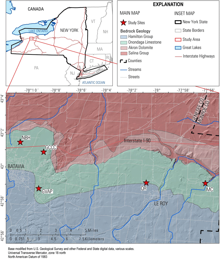
Study area and site locations (NBH – N Bennett Heights; GCCC – Genesee County Community College; GVAP – Genesee Valley Agri-Business Park; QR – Quinlan Road; MC – Mud Creek), major streams, and hillshade topography.
Geophysical Methods
A variety of geophysical methods were employed to determine which methods would work the best in the area, given the variability of overburden materials and relative uncertainty of overburden distribution. These included frequency-domain electromagnetics (FDEM), ground-penetrating radar (GPR), electrical-resistivity tomography (ERT), horizontal-to-vertical spectral ratio seismic (HVSR), and seismic refraction. For detailed information on how material properties manifest as electrical and seismic geophysical signals, see Glover (2015) and Schmitt (2015). A brief summary of data types collected is given below, while complete details including system configurations and processing methods are provided in a publicly available U.S. Geological Survey data release (DeMott and Terry, 2024). For all methods, an Emlid Reach RS2+ RTK GPS system was used to georeference data points during surveys.
FDEM instruments included a DualEM-421 and a GEM-2, each carried at about hip level. These measurements rapidly map shallow (less than 5 meters) variations in bulk soil electrical conductivity (EC) over each site and were used as reconnaissance tools to locate patterned anomalies potentially related to soil overburden type or karst drainage features. Only raw data were plotted from these instruments. Technical details of FDEM methods are presented in ASTM (2018) and Fitterman (2015).
ERT measurements used a 56-electrode SuperSting R8 system and Wenner-Schlumberger data collection geometry. Electrode spacing was either 1 meter or 2 meters, depending on the scale of the site and desired coverage of features. The purpose of the ERT measurements was to reveal spatially detailed 2D (depth slice) bulk EC variations along specific transects of interest. Such measurements may reveal void spaces filled with air (less electrically conductive compared to background soil) or water (more electrically conductive compared to background soil), or changes in overburden soil types (in freshwater settings, higher clay/fine-grained soil content often manifests as relatively higher EC). The ERT data were inverted using ResIPy, a Python wrapper for the R2 codes (Blanchy and others, 2020). Technical details of the ERT method can be found in Binley and Slater (2020).
Common offset GPR measurements were conducted using a MALÅ 160 MHz HDR shielded antenna, wheel trigger, and GX monitor. Like the FDEM surveys, GPR data were collected over larger site areas and were not necessarily limited to individual transects, though interpretation focused on lines with corresponding ERT and seismic refraction information. The purpose of the GPR measurements was to reveal radar reflections from water content related changes in shallow soils (less than 5 meters), as might occur from a void space, sudden changes in porosity, or saturation. GPR data were analyzed in ReflexW with basic processing applied (time-zero correction, dewow, and energy decay gain). Depth estimates assumed electromagnetic velocities based on diffraction hyperbola fitting from each site. Details of the GPR method and processing can be found in Neal (2004).
Limited seismic refraction tomography data were collected along a transect using a 28-geophone Geode-XT system and 14 Hz vertical geophones. Geophones were placed at a 2-meter spacing and shots were made every 4 meters along the line. The purpose of this survey was to detect changes in seismic velocity related to different soil materials and/or the soil/bedrock interface. Details of the seismic refraction tomography method can be found in Palmer (1981).
A Tromino 3G 3-component seismometer was used to collect passive seismic data suitable for HVSR analysis and single point estimates of depth to bedrock. These data were collected for approximately 20 minutes at several locations at each site and processed in the GRILLA software to estimate resonance frequency and depth to bedrock. Details of this method can be found in Nakamura (1989) and Johnson and Lane (2016). Depth to bedrock was calculated using the peak frequency, based on a regional equation from Heisig and Fleisher (2022).
Results and Discussion
N Bennett Heights
The sinkhole at N Bennett Heights is a small, subtle depression approximately 0.15 acre in area that has been identified as a patterned sinkhole by Reddy and Kappel (2010) (fig. 2). The site is at the southern end of a farm field in a vegetation buffer zone between the field and a row of houses along N Bennett Heights. The site is less than 1 mile from known sites of contamination (Reddy and Kappel, 2010; Kappel and others, 2020).
This site was the only site where all tested geophysical methods were employed. FDEM surveys were conducted with both the DualEM and GEM-2 FDEM instruments, and results indicate near-surface materials with EC in the 3–5 milliSiemens per meter (mS/m) range (fig. 2A and 2B), which likely reflects unsaturated and/or coarse material with low specific conductance. No significant trends in EC were observed between the depression and the surrounding field, although some higher values were observed with the DualEM along the southern edge, likely due to proximity to a chain-link fence.
ERT showed an increase in the resistivity around a depth of 10 feet (ft) that likely indicates transition to bedrock (fig. 2C). Some areas of higher resistivity are observed within the bedrock that may indicate karst features such as voids or weathered zones.
GPR data from the location of the ERT profile lines show a possible bedrock reflector around a depth of 6 ft (EM velocity of 0.08 meter per nanosecond (m/ns) assumed based on diffraction hyperbola fitting) inside the depression (fig. 2D). Given the shallower depth observed compared to the ERT results, this reflector may also be attributed to soil structure. Seismic refraction results also indicated an overburden thickness of 8.5 ft, with a P-wave velocity of 600 meters/second (consistent with unconsolidated material) overlying bedrock with a P-wave velocity of about 1,200 meters/second (consistent with limestone). A single HVSR measurement of moderate quality indicates bedrock around a depth of 8.5 ft. Differing bedrock depths between methods may reflect an epikarst or weathered zone at the top of the bedrock.
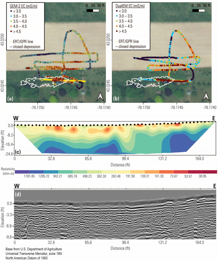
Selected geophysical results from the N Bennett Heights site, New York. The closed depression is indicated by the white polygon on (A) and (B). (A) apparent electrical conductivity from the GEM-2 48 kilohertz (kHz) band; (B) apparent electrical conductivity from the DualEM-421 4-meter horizontal coplanar coils; (C) electrical-resistivity tomography (ERT) inversion result; (D) corresponding ground-penetrating radar (GPR) radargram.
Genesee County Community College
This site is on the campus of the Genesee County Community College and is a broad closed depression with an area of approximately 3.5 acres, with a sharp, approximately 5 to 6-foot-tall scarp along the eastern edge. The central and deepest part of the depression is forested, while the southern and northern sections extend into open fields. Bedrock is close to the surface around the campus, and the sinkhole has been used by campus facilities management as a disposal site for waste rock from construction projects. FDEM, GPR, and ERT methods were employed to characterize this site.
FDEM surveys were conducted with the GEM-2 instrument, and results indicate near-surface material in the 0–3 mS/m range, with little to no measurable signal in the central part of the sink (fig. 3A). This lack of signal may be due to bedrock being very near or at the surface in the center of the sinkhole, as a higher signal was obtained around the eastern edge of the sink where the thicker soil scarp is present. GPR results indicate numerous sub-horizontal reflectors in the upper 10 ft data (EM velocity of 0.07 m/ns) that may indicate layers of bedrock and/or soil, as well as an area of lower reflection amplitudes observed in the center of the sinkhole (fig. 3C). ERT results correspond with the other observations, indicating thin soils and bedrock around a depth of 5–7 ft. An area of high resistivity in the center of the line that corresponds to the low amplitude zone observed in the GPR data, may indicate the presence of a significant karstic void near the deepest part of the sinkhole (fig. 3B).
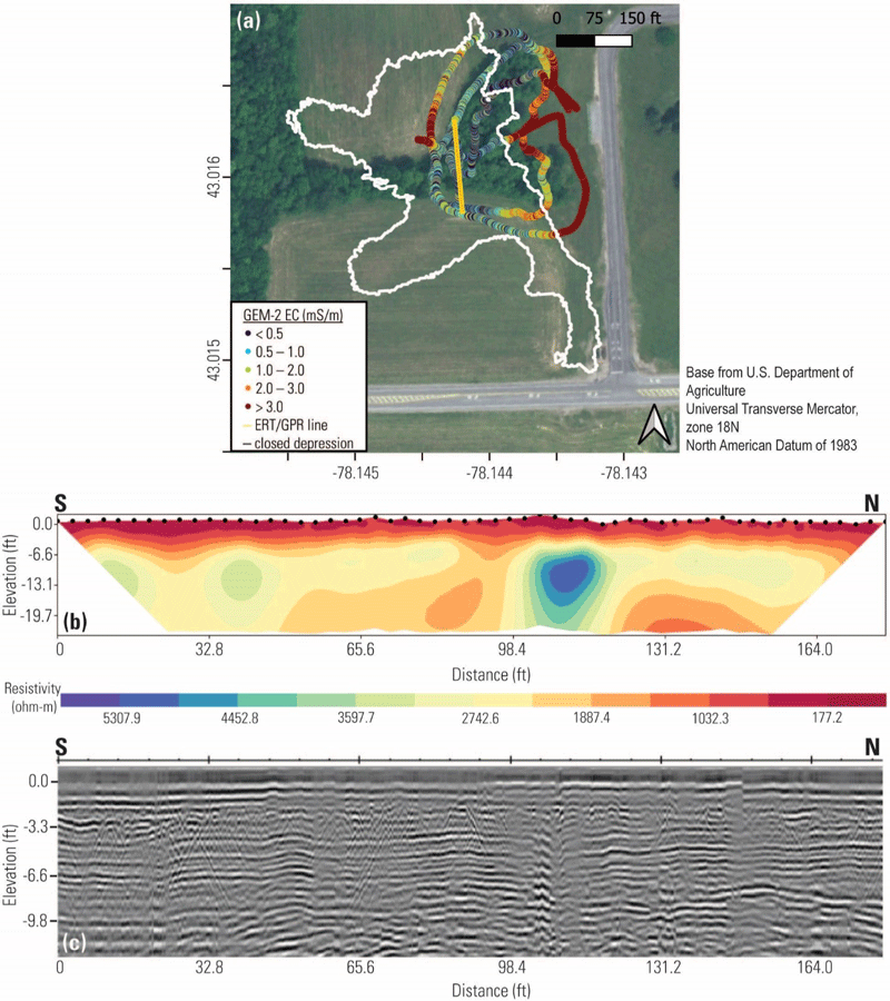
Selected geophysical results from the Genesee County Community College site, New York. The closed depression is indicated by the white polygon on (A). (A) apparent electrical conductivity from the GEM-2 48 kilohertz (kHz) band; (B) electrical-resistivity tomography (ERT) inversion result; (C) corresponding ground-penetrating radar (GPR) radargram.
Genesee Valley Agri-Business Park
The Genesee Valley Agri-Business Park depression is the largest of the sites, with an approximate area of 8 acres (fig. 4A). The depression has relatively steep sides to the north and south, with a broad flat base with trees and brushy undergrowth. A small stream enters the depression from the east, and the site floods during high rainfall events. The easternmost section of the depression is fenced and was not accessible during the study. Kappel and others (2020) and Richards and Boehm (2012) report exposed bedrock in the area; however, this was not observed in the western section of the depression covered by this study and may be limited to the eastern section. FDEM, GPR, ERT, and HVSR data were collected at this site.
Seven HVSR measurements were made at the site, four in the central axis of the depression and three on the southern rim of the depression. One measurement was taken in duplicate with consistent results; measurements were generally of moderate to excellent quality. Depth to bedrock in the center of the depression was between 7–9 ft deep, with one measurement of 19 ft deep in the eastern part of the depression. Depth to bedrock on the rim ranged from 21–39 ft deep.
FDEM surveys were conducted with the DualEM instrument. Results indicate near-surface materials in the 2–5 mS/m range, indicating unsaturated and/or coarse sediments with low specific conductance, with a zone of high EC in the eastern part of the depression (fig. 4A). EC was higher in the sinkhole than on the ridges; some anomalously high values were recorded due to proximity to the metal fencing along the eastern edge. The high EC zone, which corresponds to both the deeper HVSR measurement of 19 ft and the location of the drainage stream, was targeted for the ERT survey. The southern section of the ERT profile at the top of the break in slope (about 30 ft distance in the profile) indicates a vertical high resistivity structure, potentially indicating a fracture related to the formation of the depression (fig. 4C). ERT results from within the depression indicate a gradual transition to bedrock, with a zone of more conductive soils corresponding to the high EC zone in the FDEM survey. This area likely has a higher moisture content and finer-grained sediments than other parts of the sink due to drainage from the stream. A small dip in the section around the 150 ft point corresponds to the 19 ft HVSR measurement, possibly indicating a bedrock low.
GPR results show areas with strong shallow (less than 5 ft, based on fit EM wave velocity of 0.09 m/ns) sub-horizontal reflections most prominently visible in the western part of the depression (fig. 4B, 0–700 ft along the profile). Such reflections were not visible along the ERT line (no interpretable GPR information was available along this line). These reflections may be indicative of soil structure or may indicate the bedrock surface, albeit at somewhat shallower depths than estimated by HVSR. Possibly, areas lacking these reflections are zones where the bedrock is disturbed (for example, collapsed or weathered), such as in the eastern part of the depression.
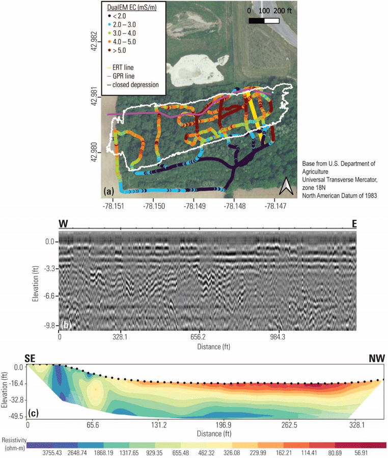
Selected geophysical results from the Genesee Valley Agri-Business Park site, New York. The closed depression is indicated by the white polygon on (A). (A) apparent electrical conductivity from the DualEM-421 4-meter horizontal coplanar coils; (B) ground-penetrating radar (GPR) radargram from west-east profile indicated in (A); (C) electrical-resistivity tomography (ERT) inversion result from south-north profile indicated in (A).
Quinlan Road
The sinkhole at Quinlan Road is a tree-lined, steep-sided swallet in the center of a very large, closed depression located in a farm field. It is the primary drainage outlet for a massive compound sink, with a man-made drainage ditch connected to the swallet to help drain the larger closed depression feature during high runoff events. Richards and Boehm (2012) interpret this as a solution sinkhole and found through use of pressure transducers that the sinkhole is subject to groundwater flooding. The Onondaga Limestone is visible in the sides of the sinkhole, starting at approximately 10 ft of depth from the surface. Due to the steep sides, hard, dry soil and exposed rock, and the narrow swallet, ERT measurements were not obtainable at this site. HVSR measurements also were not taken at this site, as bedrock is exposed in the sinkhole sides. FDEM and GPR measurements were made across the swallet and surrounding field.
Both the DualEM and GEM-2 instruments were used to collect FDEM data. The results indicate near-surface materials in the 4–10 mS/m range, with low EC values in the sinkhole and higher EC values in the fields and along the drainage ditch (figs. 5A–5C). The lower values in the sinkhole correspond to the thin dry soil and exposed bedrock, which appears to be limited to the tree-lined sinkhole area, with increasing EC values where soils are likely thicker and have higher moisture content on the fields.
GPR results surrounding the swallet (fig. 5D) indicate variable sub-horizontal reflections in the upper 6–10 ft (based on fit EM velocity of 0.1 m/ns), indicating shallow soil structure or possibly the bedrock. Increases in depth and/or absence of these reflections may indicate underlying bedrock collapse/dissolution (for example, figure 5D at 328 ft along the profile, corresponding to where the drainage ditch enters the swallet). Deeper structures in the GPR data likely represent air-reflections from the side of the GPR unit (for example, the feature at −13 ft elevation at the beginning and end of the profile on figure 5D probably corresponds to an aboveground observed metal structure). GPR profiles crossing the swallet feature itself were uninterpretable due to these air-reflections and positional inaccuracies.
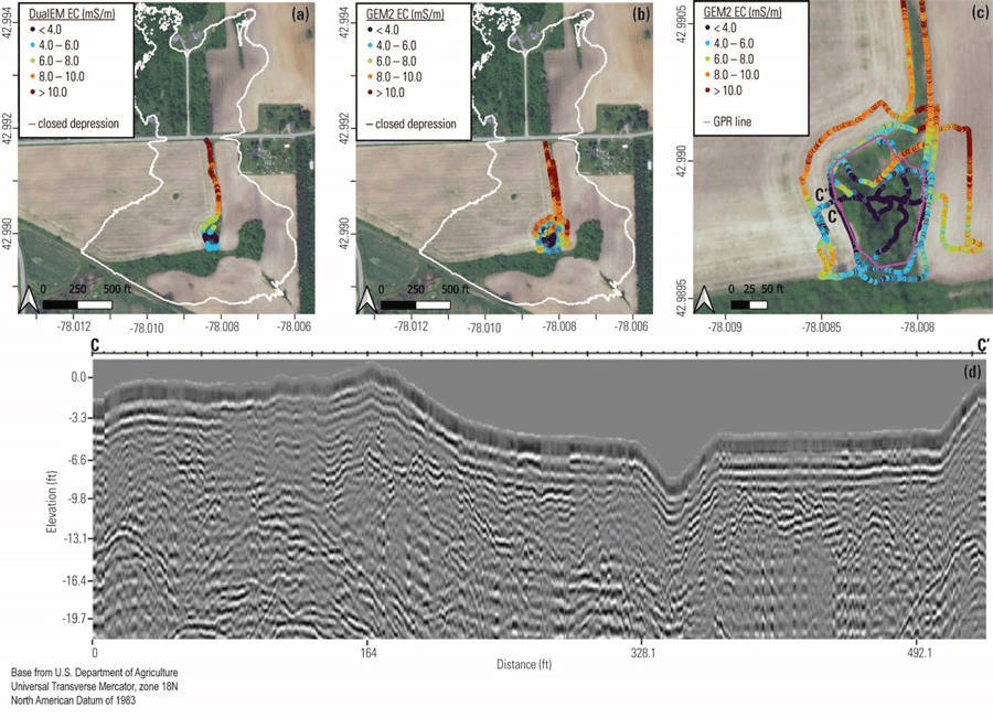
Selected geophysical results from the Quinlan Road site, New York. The closed depression is indicated by the white polygon on (A) and (B). (A) apparent electrical conductivity from the DualEM-421 4-meter horizontal coplanar coils; (B) apparent electrical conductivity from the GEM-2 48 kilohertz (kHz) band; (C) zoomed in GEM-2 electrical conductivity from the swallet area; (D) ground-penetrating radar (GPR) radargram circling the swallet feature.
Mud Creek
The Mud Creek sinkhole is a broad, relatively steep-sided depression in the streambed of Mud Creek, an intermittently flowing losing stream, just north of a stone and concrete culvert through a now-defunct railroad embankment. The sinkhole is typically water filled at normal groundwater levels, even when other parts of the streambed are dry; during the time of data collection, the region was experiencing drought and the sinkhole was also dry. The Onondaga Limestone crops out downstream, and may be exposed under the railroad culvert, but the presence of the railroad bed construction material (also Onondaga Limestone from local quarries) makes determination of this difficult. The sinkhole is filled with very wet, organic-rich mud, along with some railroad debris like old wooden ties and broken pieces of limestone and concrete. Data were collected at this site using FDEM, GPR, ERT, and HVSR instruments.
FDEM data were collected using the DualEM instrument and indicate near-surface materials in the 3–14 mS/m range (fig. 6A). In general, the sinkhole area shows elevated EC values compared to the surrounding areas upgradient and along the railroad embankment. Readings in some areas where the FDEM transect crosses over itself are not consistent, which may be due to the steep topography affecting the level of the sensor with respect to the ground surface. Higher EC in the sinkhole center may reflect the high moisture content of the organic-rich mud infill. GPR results (fig. 6C) show near-surface soil structure as well as a concave reflector consistent with the sinkhole shape, with a maximum depth of approximately 20 ft (based on fit EM velocity of 0.08 m/ns).
The ERT results show higher resistivity values in the sinkhole compared to the upgradient rim (fig. 6B). A near-vertical, very high resistivity anomaly is observed in the center of the sinkhole and is observed in both the raw data and the inverse result, indicating the presence of a significant void space in the center of the sinkhole, potentially related to an underlying solution-enhanced fracture. Closer evaluation of GPR results from this area somewhat supports this in terms of fewer visible reflections (fig. 6D). Two duplicate HVSR measurements of moderate to excellent quality were taken within the sinkhole and provided consistent results of approximately 42 ft of depth to bedrock, which is deeper than indicated by nearby quarries and outcrops downstream. These measurements may be aligned with a near-vertical feature interpreted in the ERT data where the depth to bedrock may be locally deeper than in surrounding areas.
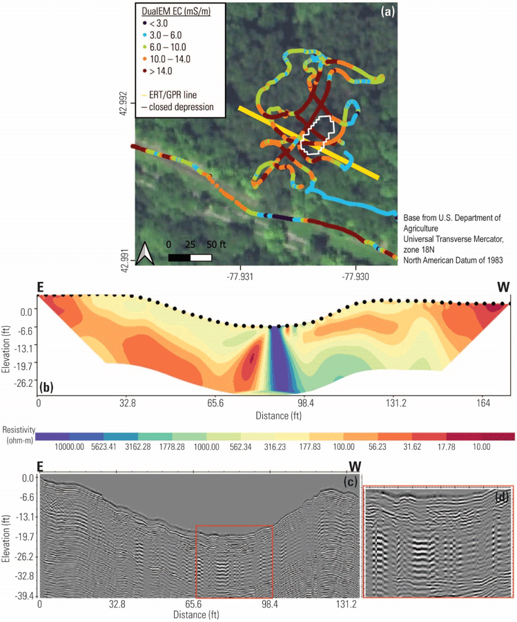
Selected geophysical results from the Mud Creek site, New York. The closed depression is indicated by the white polygon on (A). (A) apparent electrical conductivity from the DualEM-421 4-meter horizontal coplanar coils; (B) electrical-resistivity tomography (ERT) inversion result from east-west profile indicated in (A); (C) corresponding ground-penetrating radar (GPR) radargram; (D) zoom on red-outlined portion of the GPR radargram in (C).
Summary
Five karst drainage features in western New York were examined with geophysical techniques, including FDEM, GPR, ERT, HVSR, and seismic refraction, to determine the nature of the subsurface with respect to bedrock topography and glacial overburden. All five sites had sufficient physical property contrast to reveal geophysical anomalies related to karst development. FDEM methods were the most sensitive to soil property contrasts, while GPR showed detailed subsurface complexity at most sites that need additional methods to support interpretation. HVSR data were of varying quality, depending on the depth to bedrock and nature of the fill material. ERT was the most useful method for providing interpretable information about karst features, revealing potential bedrock voids and fractures. These geophysical data are available in a USGS data release. Future studies in the region, such as tracer tests or aquifer models, would benefit from multiple geophysical techniques to evaluate these features and gain insight into the nature of karstification.
Acknowledgments
This study was conducted in cooperation with the New York State Department of Environmental Conservation. The authors would like to thank the site property owners for allowing access to the study sites. Robin Glas and Jenna Klein assisted with the field data collection.
Any use of trade, firm, or product names is for descriptive purposes only and does not imply endorsement by the U.S. Government.
References Cited
Blanchy, G., Saneiyan, S., Boyd, J., McLachlan, P., and Binley, A., 2020, ResIPy, an intuitive open source software for complex geoelectrical inversion/modeling: Computers & Geosciences, v. 137, 104423, https://doi.org/10.1016/j.cageo.2020.104423.
DeMott, L.M., and Terry, N., 2024, Geophysical data for assessment of karst drainage features in Genesee County, New York: U.S. Geological Survey data release, https://doi.org/10.5066/P13GSEAP.
Heisig, P.M., and Fleisher, P.J., 2022, Glacial geology and hydrogeology of valley-fill aquifers in the Oneonta area, Otsego and Delaware Counties, New York: U.S. Geological Survey Scientific Investigations Report 2022–5069, 35 p., 1 pl., https://doi.org/10.3133/sir20225069.
Johnson, C.D., and Lane, J.W., Jr., 2016, Statistical comparison of methods for estimating sediment thickness from horizontal-to-vertical spectral ratio (HVSR) seismic methods—an example from Tylerville, Connecticut, USA, in Symposium on the Application of Geophysics to Engineering and Environmental Problems, Denver, Colorado, March 20–24, 2016, Proceedings: Denver, Colorado, Environmental and Engineering Geophysical Society, 7 p.
Kappel, W.M., Reddy, J.E., and Root, J.C., 2020, Statewide assessment of karst aquifers in New York with an inventory of closed-depression and focused-recharge features: U.S. Geological Survey Scientific Investigations Report 2020–5030, 74 p., https://doi.org/10.3133/sir20205030.
Reddy, J.E., and Kappel, W.M., 2010, Compilation of existing hydrogeologic and geospatial data for the assessment of focused recharge to the carbonate-rock aquifer in Genesee County, New York: U.S. Geological Survey Scientific Investigations Map 3132, 17 p., 20 sheets, https://pubs.usgs.gov/sim/3132/.
Richards, P.L., and Boehm, D., 2012, Adapting SWAT for the assessment of thinly-soiled karst and sinkhole features: Oatka Creek Watershed Committee Report, 44 p., https://oatka.org/wp-content/uploads/Richards_2011_WRI_FinalReport.pdf.
Sporleder, B.A., DeMott, L.M., Fisher, B.N., Keto, D.S., and Fisher, S., 2021, Geospatial data to assess karst aquifer systems between Albany and Buffalo, New York (ver. 4.0, January 2024): U.S. Geological Survey data release, https://doi.org/10.5066/P9AYMP94.
Cave Climate 100 Meters Below the Surface in the Pseudokarst of the Kilauea Southwest Rift Zone, Hawaii
Abstract
Kīlauea volcano hosts numerous pit craters that are inferred to have formed in competent bedrock (lava flows with minor tephra and other sediments), including Wood Valley Pit Crater. The Wood Valley Pit Crater is a 50-meter-deep, nearly circular pit that includes access to a cave entrance, which provides an opportunity to monitor cave climate throughout a cave that is ordinarily inaccessible. Cave climate observations in this volcanic pseudokarst area included cold trapping, cave breathing, possible effects from geothermal heating, and possible atmospheric thermal tide-induced cave fog.
Introduction
Kīlauea volcano hosts numerous pit craters that are inferred to have formed in competent bedrock (lava flows with minor tephra and other sediments), and some of these pits did not form along large normal faults or grabens. These pits are located along zones of ground cracking, and patterns of these ground cracks were used by Okubo and Martel (1998) to demonstrate the presence of large opening-mode fractures below the pits. These zones of ground cracking exhibit predominantly horizontal extensional displacements, with little, if any, vertical displacement characteristics of normal faults. The pit craters are also located within the volcano’s rift zones and at the summit region, both areas where magma flow is known to occur in dikes or larger conduits (Neal and others, 2019).
Fourteen pit craters and pit crater complexes (clusters of multiple overlapping pit craters) are known to occur along Kīlauea’s East Rift Zone (ERZ), with two of these no longer visible due to infilling by lava flows associated with the 1969–1974 Mauna ‘Ulu eruption (U.S. Geological Survey, 2023). Kīlauea’s summit region experienced multiple episodes of pit crater formation during the recent (2008–2018) activity (Patrick and others, 2020; Poland and others, 2021). The Southwest Rift Zone (SWRZ) contains approximately 15 pit craters and pit crater complexes, the majority of which are located both up-rift and down-rift of the Great Crack, an eruptive fissure that was active in 1823 (Stearns, 1926; Stone, 1926). The total number of pit craters along the SWRZ is approximate because several of the pit crater complexes adjacent to the Great Crack coalesce with large aperture (greater than 10 meters (m) wide), non-eruptive, talus-filled fissures, and individual pits become difficult to distinguish from collapsed sections of those fissures.
Pit craters of Kīlauea’s SWRZ appear to have formed in competent bedrock and were not associated with large normal faults; most of these pit craters are known to contain caves at the pit bottoms (Okubo and Martel, 1998; Halliday, 2002; Favre, 2014; Coons, 2016; Cushing, 2016). Only two ERZ pit craters, Devils Throat (Jaggar, 1947) and Lua Niʻi (Macdonald and Eaton, 1964), are known to have contained caves at their bottoms. However, the caves within these two pits are no longer visible because their entrances have been buried by talus from the pit walls.
Wood Valley Pit Crater Cave
The floor of Wood Valley Pit Crater (WVPC) can only be accessed via rappelling. At ground level, WVPC is approximately 35 m x 28 m in diameter and is elongate in the northeast-southwest direction. Inside the pit, the base is approximately 60 m x 40 m in diameter and is elongate in the north-south direction. The pit’s shape is that of an elliptic conical frustum and is approximately 41 to 47 m deep.
The walls of WVPC comprise a sequence of fractured basalts, primarily ‘a‘a flows. The floor of the pit consists of poorly sorted, angular blocks of basalt that are about 2 m in length or less. These blocks appear consistent with the ‘a‘a flows exposed in the pit walls and therefore are interpreted to have been derived through collapse of those walls.
The WVPC and the entire length of its known cave system was first described by Favre (1993) and re-surveyed by Favre (2014) using a handheld laser rangefinder and magnetic compass. These surveys revealed that the entrance to this cave is located at the base of the northeast wall of the pit. The cave is roughly linear in map view and trends northeast-southwest, which is parallel with the local orientation of the SWRZ. The horizontal extent of the cave is approximately 475 m, and at its deepest point is approximately 60 m below the floor of WVPC.
Favre (1993, 2014) revealed an uncommon origin for the WVPC cave. They noted that the walls and ceiling of the cave were coated in lava dripstone, as is often observed in lava tubes and eruptive fissures. Further, the largest room in the cave, informally named “Salle du Four” translated as the “Oven Room,” is shown to have an ovate (Favre, 1993) to tabular (Favre, 2014) shape in cross section. Favre (1993, 2014) interpreted this cave as being the top of a partially drained dike, with the glassy dripstone and ‘a‘a, and pahoehoe floor composing the basalt (magma) that drove the dike’s formation. Although Walker (1988), Okubo and Martel (1998) and others have interpreted Kīlauea’s pit craters to have formed above partially drained dikes, examples where such dikes are known are uncommon. Lua Nii (Macdonald and Eaton, 1964) and “Pit H” along the Great Crack (Okubo and Martel, 1998; Halliday, 2002; Coons 2016) are the only other known examples of pit crater/cave systems that formed above and within partially drained dikes.
Methodology and Data Collection
Both cave geometry and climate data were collected in stages over a period of several years (Cushing and others, 2024). Each visit to the cave was typically 7–10 days. During each visit, climate data were extracted from the pressure, temperature, and humidity data, while part of the cave was surveyed using a three-dimensional mapping system. A description of the approach for the collection of both types of data follows.
A tripod-mounted three-dimensional mapping system was used to map the shapes of WVPC and two of the largest rooms in its cave, as well as to map the locations of the pressure, temperature, and humidity sensors therein. The mapping system consists of an infrared laser rangefinder with an integrated inclinometer and an optical azimuth encoder (Impulse 200 and TruAngle from Laser Technology, Inc.) mounted on top of a surveying tripod. This system has the key advantage of being able to be broken down into small, lightweight components that can be secured in moderately sized hard cases for transport to the bottom of WVPC and through the tight squeezes of the cave. The laser rangefinder records target locations in spherical coordinates (range, azimuth, inclination) relative to the focal point of its receiver, which are subsequently converted to Cartesian coordinates. Using this system, the entirety of WVPC was remapped and a total of about 75 m of the approximately 475-meter length (Favre, 2014) of its cave.
Temperature (rock and air), relative humidity, and barometric pressure data were collected at the cave entrance (located at the bottom of the pit) and throughout the cave network (fig. 1; table 1). An entire year of data were collected for the cave walls surrounding one of the cave entrances and the upper portion of the cave, and about 6 months of data for the lower portion of the cave, which included the horizontal basaltic dike. Unfortunately, wind data from either inside the cave or near the entrance were not collected.
Temperature and humidity data can be separated by two date ranges: (1) 10/19/2012–4/18/2013, and (2) 4/18/2013–11/30/2013. The first dataset range only included pit and upper cave observations, while the second dataset range included the pit and the entire cave network. Pressure data, acquired at 10-minute intervals, were available from 10/22/2012–8/5/2014. The pressure sensor was occasionally relocated. A second pressure sensor acquired data at 30-second intervals from near the cave entrance from 4/20/2013–9/19/2013.
Temperature: Rock and air temperatures were concurrently recorded using a HOBO data logger U23-003s, with two external probes. One probe was inserted into a small hole drilled into the rock (channel 1), while the other probe (channel 2) was left exposed to the air. These sensors have an absolute accuracy of 0.2 degree Celsius (°C) and a relative accuracy of 0.02 °C. The digitization level as measured from the data was determined to be 0.023 °C, which is comparable to the stated relative accuracy.
Humidity: Humidity was measured throughout the cave complex using a HOBO data logger U23-001s, where air temperature and humidity are measured with internal sensors. These sensors were usually colocated with one of the U23-003 data loggers. These sensors are not accurate at relative humidities above 95 percent, otherwise they have an accuracy of 2.5 percent.
Pressure: Barometric pressure was measured near the cave entrance and at the back of the cave using HOBO S-BPA-CM10 pressure sensors. The sensor accuracy is plus or minus 3.0 millibars (mbar) over the full pressure range at 25 °C. The data resolution (digitization error) is 0.1 mbar, which is consistent with the data collected.
Table 1.
Sensor locations and data types in Wood Valley Pit Crater Cave.See figure 1 for sensor locations on the cave map and in the cave.
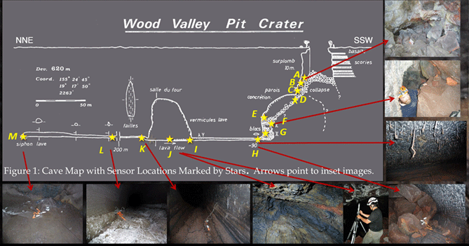
Map of sensor locations in Wood Valley Pit Crater Cave along with context images. This is a scaled cross-section diagram (modified from Favre, 1993; Cushing and others, 2015). The yellow stars indicate approximate locations of the sensors. The yellow letters (A–M) adjacent to the stars identify the sensor location in table 1. The red arrows point to context images that either show the sensor placement or nearby interesting features. All images, except for the “Salle du Four” image, were taken by Tim Titus. The image of “Salle du Four” (J) was taken by G. Favre and his team.
Temperature Data and Trends
Four sensors were placed around the east entrance to the cave. Each sensor has two external probes, so one was inserted into a drill hole in a rock while the other was placed to better record air temperature. Figure 2 shows that the rocks exceeded 20 °C during the winter months when they received direct sunlight. Air temperatures showed that nighttime temperatures, especially during the winter (and rainy) months, often were cooler than the rocks. A comparison to figure 3 shows that cold trapping likely occurs as the cave cools with depth.
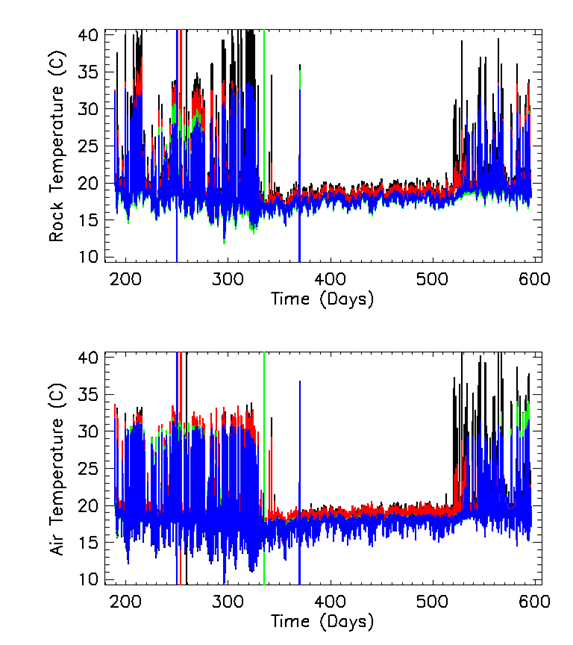
Surface temperature data from near the east cave entrance in Wood Valley Pit Crater (location A2, table 1, fig. 1), showing rock temperature (top), and air temperature (bottom), in degrees Celsius (C). The time axis shows the number of days since April 13, 2012. Temperatures above 20 °C were due to direct sunlight on the rock and sensor, which only occurs during the winter months. Air temperatures drop below rock temperatures at night, allowing cold trapping to occur. The black, red, green, and blue lines indicate different surface sensors at location A2 (fig. 1, table 1).
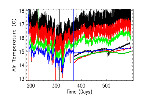
Air temperature data throughout the Wood Valley Pit Crater Cave. The time axis shows the number of days since April 13, 2012. Solid black (location B), red (location C), green (location D), and blue (location E) lines show the upper portion of the cave passage. Dashed black (location G), red (location H), green (location J), and blue (location M) lines show the lower portion of the cave passage including the horizontal basaltic dike. Air temperature in degrees Celsius (C).
Relative Humidity Data and Trends
The cave air spends more time saturated as one descends deeper underground. By the time one gets to the horizontal dike, the air is consistently saturated (fig. 4).

Relative humidity data throughout the Wood Valley Pit Crater Cave. The time axis shows the number of days since April 13, 2012. Black (location B), red (location C), green (location D), blue (location E), and magenta (location F). As one gets deeper into the cave, the air remains at 100 percent saturation more of the time.
Barometric Pressure Data and Trends
Barometric pressure was measured about 10 m below the west cave entrance and at the end of the horizontal dike. These data are shown on figure 5. The pressure offset is consistent with an elevation change of about 40 m. The phase difference between the two sets of measurements was negligible.

Barometric pressure data at two locations in the Wood Valley Pit Crater Cave. The black curve shows the pressure measured about 10 meters below the west cave entrance (location B in table 1, fig. 1), and the red curve shows the pressure measured at the end of the horizontal dike (location M in table 1, fig. 1). The pressure offset is due to elevation difference. There was negligible phase difference between the pressure curves. Pressure in millibars (mBars).
Atmospheric Thermal Tides
Fourier transform analysis of the barometric pressure data showed the influence of atmospheric thermal (or solar) tides (fig. 6).
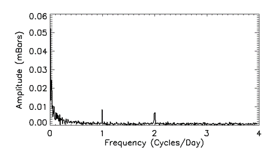
Fourier transform analysis of the barometric pressure data shown on figure 5 for the west cave entrance (location B) and at the end of the horizontal dike (location M). The S1 and S2 solar (atmospheric thermal) tides are obvious as amplitude spikes at one and two cycles per day. Amplitude in millibars (mBars).
Cave Breathing and Wind
Air flow was felt when the “low crawl” tunnel that connected the “Oven Room” to the back passage of the dike was traversed. Unfortunately, it was not possible to measure or monitor the air-flow rate or direction. However, the presence of air flow does indicate that the cave was breathing. Because the cave geometric configuration appeared to be static (a single entrance that is above the subsurface void), the air flow was likely pressure driven.
Cave Fog
Part of the data collection in the cave was the use of an infrared laser rangefinder. Survey data of the “Oven Room” from the rangefinder often produced a scattering of distances instead of clean consistent distances to the room’s wall and ceiling. It was realized that the laser beam was likely reflecting off water droplets suspended in the cave air (cave fog), and that the number or density of droplets varied throughout the day. This hypothesis was anecdotally supported by images (fig. 7) taken by Tim Titus of Chris Okubo at two different times of day, one where the air is relatively clear and the second where there appear to be suspended droplets. The hypothesis is further supported by comparing the observed air temperature to expected temperature changes based on pressure and the ideal gas law (fig. 8) if no phase change occurred. The apparent stability of the observed temperature when compared to the pressure-derived temperature suggests that latent heat was exchanged. This is possible as the air was always saturated. Further analysis is needed, but it’s possible that cave fog was observed 100 m underground, driven by solar tides.
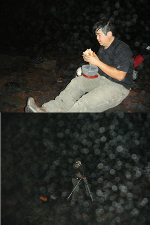
Cave fog images in the Oven Room of Wood Valley Pit Crater Cave, showing a view of Chris Okubo with relatively few “spots” (top), and an image of Chris taking laser distance data at a time when there were numerous spots observed (bottom). These “spots” may be cave fog. Photographs taken by Tim Titus.
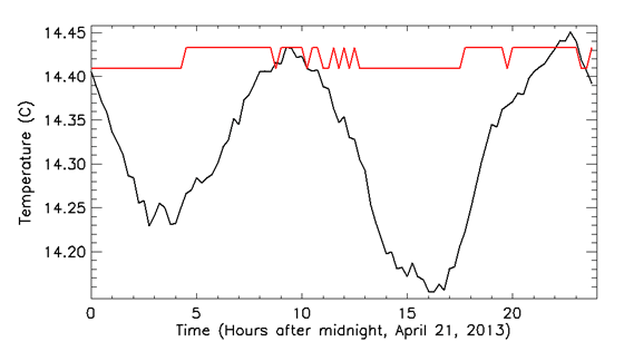
Air temperature vs. time of day in the “Salle du Four” section of the Wood Valley Pit Crater Cave. The black line shows the temperature predicted from the ideal gas law under adiabatic conditions based on measured pressure. The red line shows the observed temperature. The isothermal behavior is consistent with temperature buffering at the phase changes related to the formation and dissipation of fog. Temperature in degrees Celsius (C).
Summary
Wood Valley Pit Crater Cave provided an opportunity to monitor cave climate throughout a cave that is ordinarily inaccessible (access to a horizontal dike that is about 100 meters underground). The entrance of the cave is in the bottom of a 50-meter-deep nearly circular pit, likely formed from collapse. The cave passage continued 50 meters farther underground from the entrance, providing access to a horizontal dike that extends for hundreds of meters.
The cave climate appeared to be mainly driven by external pressure changes from weather systems and solar tides, the flow of cooler air into the cave (cold trapping), percolation events, and possible effects from geothermal heating.
Cave “fog” was observed to form and dissipate in the lower part of the cave—the horizontal basaltic dike—due to pressure-induced adiabatic expansion/compression and the air remaining saturated with water vapor year-round.
Acknowledgments
This project was partially funded through the National Atmospheric and Space Administration (NASA) Exobiology Program. The authors would like to thank G. Favre and his team for having discovered this cave and their assistance in accessing the lower sections of the cave. The authors also thank Ken Fujiyama for permission to conduct this field research during the period he was leasing the land from the State of Hawaii.
Any use of trade, firm, or product names is for descriptive purposes only and does not imply endorsement by the U.S. Government.
References Cited
Coons, D., 2016, Cave exploration within the Great Crack of Kīlauea volcano: Proceedings of the 17th International Vulcanospeleology Symposium, http://www.cavepics.com/IVS17/COONSI.pdf.
Cushing, G., 2016, Hawaiʻi analog pit crater data: https://astrogeology.usgs.gov/search/map/Earth/HawaiiPitCraters/Hawaii_Analog_Pit_Crater_Data.
Cushing, G.E., Okubo, C.H., and Titus, T.N., 2024, Cave climate data in Wood Valley pit crater, Hawai'i: U.S. Geological Survey data release, https://doi.org/10.5066/P13RSSZL.
Halliday, W.R., 2002, Caves of the Great Crack, Kilauea volcano, Hawaii: AMCS Bulletin, v. 19, p. 57, http://www.vulcanospeleology.org/sym10/ISV10p5.pdf.
Jaggar, T.A., 1947, Origin and development of craters: Geological Society of America Memoirs, v. 21, https://doi.org/10.1130/MEM21.
Macdonald, G.A., and Eaton, J.P., 1964, Hawaiian volcanoes during 1955: U.S. Geological Survey Bulletin 1171, p. 98–101, https://doi.org/10.3133/b1171.
Okubo, C.H., and Martel, S.J., 1998, Pit crater formation on Kilauea volcano, Hawaii: Journal of Volcanology and Geothermal Research, v. 86, no. 1, p. 1–18, https://www.sciencedirect.com/science/article/abs/pii/S0377027398000705.
Patrick, M., Johanson, I., Shea, T., and Waite, G., 2020, The historic events at Kīlauea Volcano in 2018—summit collapse, rift zone eruption, and Mw 6.9 earthquake—preface to the special issue: Bulletin of Volcanology, v. 82, no. 46, https://doi.org/10.1007/s00445-020-01377-5.
Poland, M.P., Miklius, A., Johanson, I.A., and Anderson, K.R., 2021, A decade of geodetic change at Kīlauea’s summit—observations, interpretations, and unanswered questions from studies of the 2008–2018 Halemaʻumaʻu eruption, chap. G of Patrick, M., Orr, T., Swanson, D., and Houghton, B., eds., The 2008–2018 summit lava lake at Kīlauea Volcano, Hawaiʻi: U.S. Geological Survey Professional Paper 1867, 29 p., https://doi.org/10.3133/pp1867G.
U.S. Geological Survey, 2023, 1969–1974 Maunaulu eruption: Kilauea, https://www.usgs.gov/volcanoes/kilauea/science/1969-1974-maunaulu-eruption.
Walker, G.P.L., 1988, Three Hawai'ian calderas—an origin through loading by shallow intrusions?: Journal of Geophysical Research, v. 93, issue B12, p. 14773–14784, https://agupubs.onlinelibrary.wiley.com/doi/abs/10.1029/JB093iB12p14773.
Ice Cave Climate Monitoring at Sunset Crater National Monument, Arizona
Abstract
The purpose of this project was to monitor the cave climate of Bonito Flow Ice Cave in Sunset Crater National Monument, Arizona. The main purpose of the climate monitoring was to determine if the Ice Cave was still an “ice cave,” in other words, a cave that contains perennial ice. The data acquired from March 2, 2021, to December 13, 2022, consisted of air temperature, relative humidity, and barometric pressure throughout the cave and included temperature and humidity measurements outside the cave, but near the entrance. This cave is considered a sacred spot by at least three southwestern Tribes because it was a historical source of ice and continues to be a place for pilgrimages and ceremonies.
Sensors were distributed throughout the cave with a focus on a large ice puddle that forms on the cave floor during the winter months. Air temperatures on the cave floor often showed decreases that corresponded to times when the outside air temperatures were below that of the cave air temperature, indicating the flow of colder air into the cave. The cave air was saturated with water vapor most of the time. An air temperature gradient existed between the cave floor and ceiling; this gradient was greatest during the summer. Hoarfrost was observed on the cave walls and ceiling, indicating that the rock was at or below freezing temperatures.
Sunset Crater Bonito Flow Ice Cave may still be an ice cave, but additional monitoring and analysis are needed. The visible presence of ice at the ice puddle occurred for about 11 out of 12 months each year, but perennial ice may still exist just below the rocky cave floor. The temperature of the floor never rose above a few degrees Celsius, and once freezing cold air from the surface flowed back into the cave, it dropped to below freezing. Therefore, these data indicate that this cave is a static ice cave.
Introduction
Ice caves (rock-hosted caves that contain perennial ice or snow) are threatened by global warming. The issue of global climate change has been a topic of public debate and scientific discussion over the last few decades. The impact of climate change on cave climate is complex. How a cave climate responds to changing surface conditions is multivariate and depends on a complex interplay among outside air temperature (especially minimum diurnal and seasonal air temperatures); surface temperatures (this includes effects caused by changes in vegetation); the timing, amount, and deposition mode (rain vs. snow) of precipitation; and the cave structure (configuration) itself. For example, warming daytime air temperatures may have minimal effect on cave temperature if nighttime and winter above-ground air temperatures remain sufficiently cold and continue to flow into the cave (pushing warmer air out), keeping the cave temperature at or below freezing (in other words, cold trapping; Williams and McKay, 2015).
One such cave was initially formed by the Bonito Lava Flow in Sunset Crater National Monument during the Sunset Crater volcanic eruption that occurred about 1066 (Houk and Scott, 1995). This cave became a source for perennial ice and was used by local indigenous populations (Stoffle and Van Vlack, 2022), and later, by settlers of European descent (Houk and Scott, 1995). Because the cave was a reliable source for ice, some southwestern tribes (Hopi, Zuni, Southern Paiute) considered the cave a sacred spot, and it continues to be a destination for spiritual pilgrimages and ceremonies (Hopi, Zuni) and celebrated in migration songs (Zuni) (Stoffle and Van Vlack, 2022). To protect the cave, the entrance has a locked gate and is only accessible with a permit from Sunset Crater Monument staff and permission from the Hopi and Zuni tribes. Figure 1 shows the local terrain, with the cave entrance in the background.
Our primary purpose for climate monitoring was to determine if Bonito Flow Ice Cave was still an ice cave. Data acquired consisted of air temperature, relative humidity, and barometric pressure throughout the cave, accompanied with temperature and humidity measurements outside the cave, near the entrance.
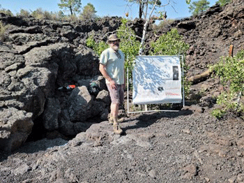
Glen Cushing standing near the entrance to Bonito Flow Ice Cave. The cave has a locked gate so when data collection occurs, someone guards the gate to prevent unauthorized entrance. The presence of a team member at the gate also served as an opportunity for public outreach. A portable poster frame from PVC pipe was constructed that could be easily assembled, disassembled, and carried in a backpack. Photograph taken by Timothy Titus, U.S. Geological Survey.
Data Collection Locations Within the Cave
Data collection was conducted from March 2, 2021, to December 13. 2022, and consisted of air temperature, relative humidity, and barometric pressure measurements. Temperature and humidity were collected outside of the cave (locations 1 and 2 in table 1), and at several places within the cave (locations 3–8 on figure 2 and table 1). Pressure data were collected at three locations within the cave (locations 3–5 on figure 2 and table 1). Additional weather data were collected approximately 800 meters north of the cave site, providing useful context for cave data interpretation (Cushing and others, 2023). Photographs from locations shown on figure 2 are provided as figs. 3–8).
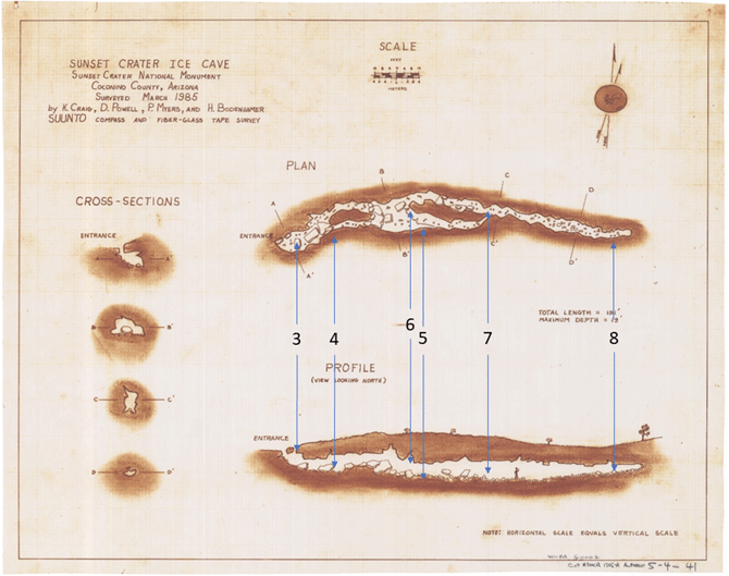
Map of Sunset Crater (Bonito Flow) Ice Cave. The length of the cave is 69 meters. The scale markings are plus or minus 4, 8, and 12 feet on top and plus or minus 1, 2, 3, and 4 meters on the bottom. The numbers indicate locations where data were collected. Table 1 provides additional location descriptions. Locations 1 and 2 are outside of the cave. Modified from 1985 National Park Service map.
Table 1.
Sensor data types and location descriptions for sites shown on map of Sunset Crater Bonito Flow Ice Cave (refer to fig. 2).| Sensor Serial Number | Data Type | Location in figure 2 | Location Description |
|---|---|---|---|
| 20987823 | Temperature/Humidity | 1 | Outside, tree – 2 meters above ground |
| 20987824 | Temperature/Humidity | 2 | Outside cave on top of entrance |
| 21018958 | Pressure | 3 | Inside cave entrance on a ledge |
| 20987825 | Temperature/Humidity | 3 | Inside cave entrance on a ledge |
| 21018955 | Pressure | 4 | Cave floor – ice puddle location |
| 20987826 | Temperature/Humidity | 4 | Cave floor – ice puddle (air) |
| 20987827 | Temperature/Humidity | 4 | Cave floor – ice puddle (rock) |
| 20987828 | Temperature/Humidity | 4 | Cave floor – ice puddle (ice) |
| 21018952 | Pressure | 5 | Mid-cave floor |
| 20987829 | Temperature/Humidity | 5 | Mid-cave floor |
| 20987830 | Temperature/Humidity | 6 | Mid-cave ceiling |
| 9702168 | Temperature/Humidity | 7 | T-intersection, 1 meter above cave floor |
| 9702169 | Temperature/Humidity | 8 | Near back of the cave |
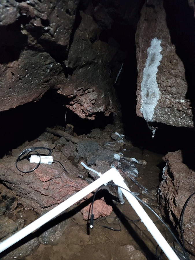
Ice puddle monitoring in Bonito Flow Ice Cave (location 4 on figure 2 and table 1). A PVC pipe constructed tripod was used to hang a sensor probe above the ice puddle to monitor air temperature/humidity. Additional temperature/humidity sensors were located at this site to measure the ice and rock surface temperature and humidity. Photograph taken by Timothy Titus, U.S. Geological Survey.
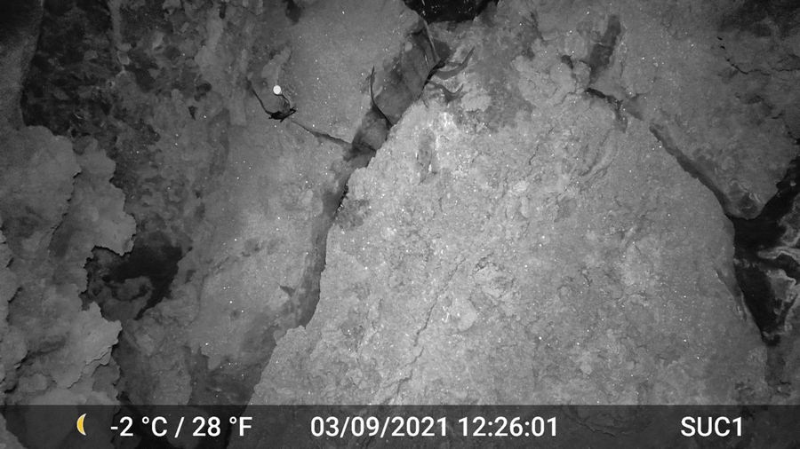
Air temperature and humidity monitoring near the cave ceiling in Bonito Flow Ice Cave. The sensor was attached to a preexisting thermometer that was mounted in the ceiling. This image was acquired using a game camera (Cushing and others, 2024).
Ice Observed—Stalagmites, Stalactites, Ice Puddle, and Hoarfrost
The presence of icicles (stalactites) indicates that percolated water from surface snowmelt was a significant source of water for Bonito Flow Ice Cave. Ice stalagmites often formed beneath the ice stalactites. The lowest part of the cave typically had a “puddle” of ice (location 4 on figure 2 and table 1; fig. 7) that was visible at least 11 months of each year. The water source was likely from percolated snowmelt that did not immediately freeze or meltwater from the ice stalagmites (fig. 5) and stalactites (fig. 6). Hoarfrost, the result of water vapor condensing directly on the cave walls and ceiling, was also observed seasonally (late winter) (fig. 8).
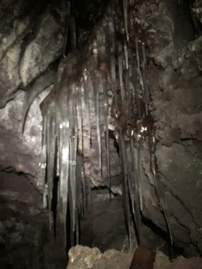
Ice stalactites formed on the cave ceiling from percolation of snowmelt in Bonito Flow Ice Cave. Photograph taken by Amber Gullikson, U.S. Geological Survey.
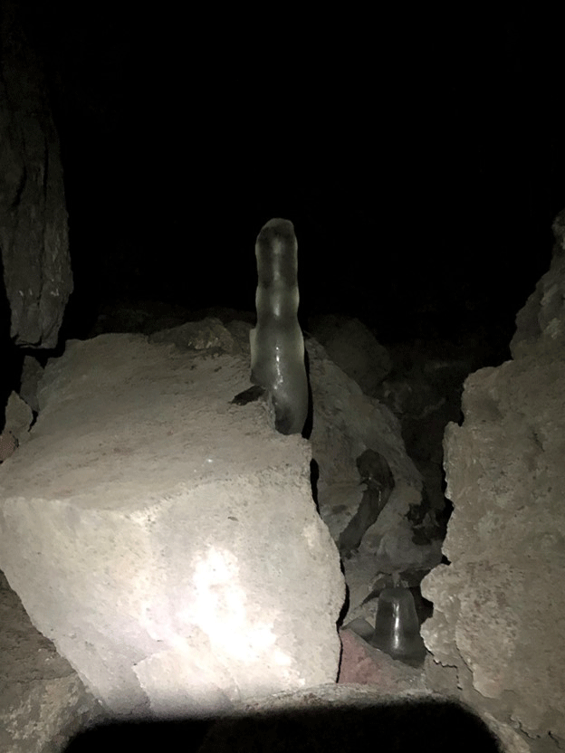
Ice stalagmite formed from percolation of snowmelt in Bonito Flow Ice Cave. Photograph taken March 2, 2021, by Amber Gullikson, U.S. Geological Survey.
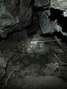
Image of the ice puddle in Bonito Flow Ice Cave while frozen. The clear substance that appears to be water is actually clear ice. Photograph taken by Kaj E. Williams, U.S. Geological Survey.
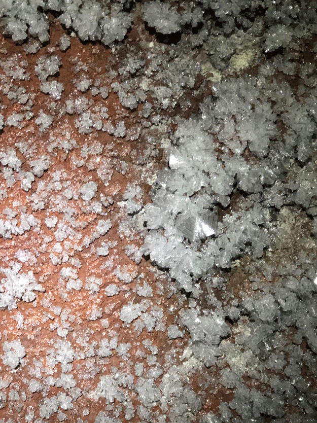
Hoarfrost on the cave wall in Bonito Flow Ice Cave. Photograph taken March 2, 2021, by Amber Gullikson, U.S. Geological Survey.
Climate Data Collected—Temperature, Humidity, and Pressure
Figure 9 shows nearly 2 years of climate data collected in Bonito Flow Ice Cave for 2021–2022. Data gaps occurred due to either sensor failure or from the data logger memory becoming full. The general trends were repeatable between the 2 years. Generally, the amplitude of temperature variations progressively decreased past the cave entrance. The exception was the cave ceiling (location 6, fig. 2 and table 1), which nearly tracks the entrance temperature. Relative humidity variations were observed at the entrance. The remainder of the cave was saturated almost all year. The exceptions were the cave ceiling, and possibly during periods when the temperature of the cave was below freezing. However, relative humidity measurements at temperatures below freezing are suspect due to instrument limitations. The cave is a static ice cave (in other words, no flow-through) (Williams and McKay, 2015), and is only 69 meters in length. As such, the three pressure measurements generally tracked each other.
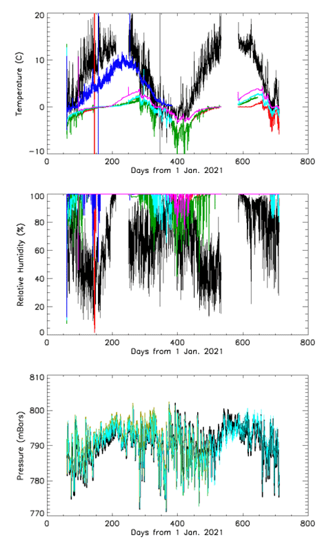
Climate data collected inside Bonito Flow Ice Cave, 2021–2022, showing air temperature, in degrees Celsius (C) (top), relative humidity, in percent (middle), and barometric pressure, in millibars (bottom). The lines represent data from inside the cave entrance (black), the ice puddle (air [red], rock [brown], ice [green]), mid-cave floor (cyan), mid-cave ceiling (blue), and near the back of the cave (magenta) at the T-intersection. Relative humidity values less than 100 percent, when the air temperature is below freezing, may not be accurate due to limitations of the sensor.
Entrance Data and Trends
The cave entrance (location 2 on figure 2 and table 1) temperature and humidity data are generally consistent between the 2 years (fig. 10). Near-total saturation (100 percent relative humidity) occurred when the air temperature was near freezing and during the summer period of the monsoons, typically July–August.
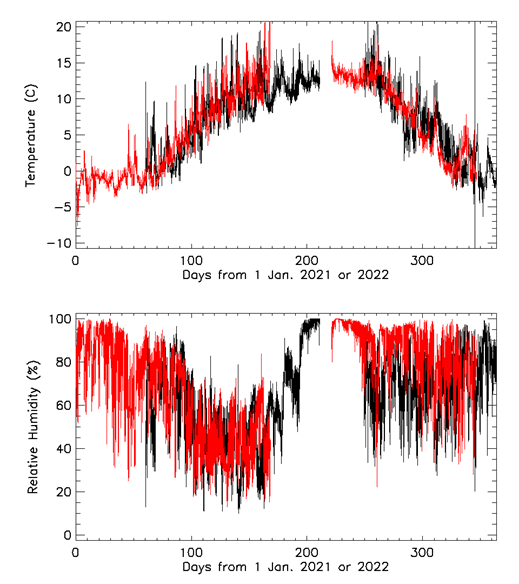
Climate data collected from the entrance of Bonito Flow Ice Cave, 2021–2022, showing air temperature, in degrees Celsius (C) (top), and relative humidity, in percent (bottom). Black lines indicate 2021 and red lines indicate 2022.
Ice-Puddle Data
The ice puddle is location 4 on figure 2 and table 1. Three temperature and humidity sensors were placed near this location, and the multi-year data are shown on figure 11. This is likely the location of any perennial ice, even though there were about 30 days in early autumn when the cave floor appeared free of visible ice and standing water (at least for 2022). Perennial ice could be present just under the rocky cave floor, as floor temperatures return quickly to freezing temperatures.
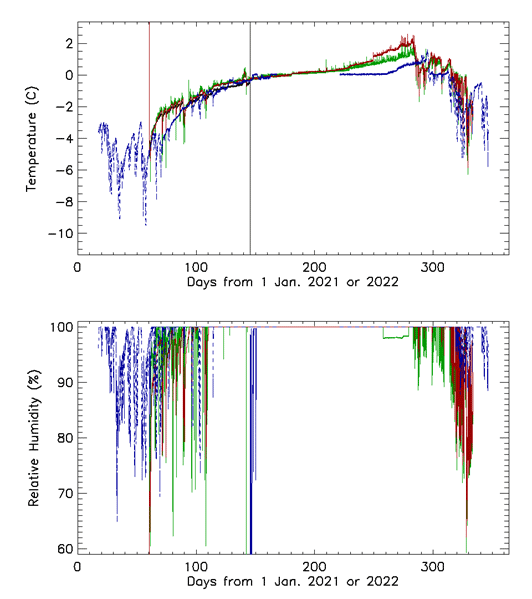
Climate data collected from the ice puddle in Bonito Flow Ice Cave, 2021–2022, showing air temperature, in degrees Celsius (C) (top), and relative humidity, in percent (bottom). Red, green, and blue lines indicate data were collected from the surface of a rock, the ice, and the air, respectively. Solid lines indicate 2021 and dashed lines indicate 2022.
Mid-Cave Data
Farther into the cave passage, past the ice puddle, is the mid-cave section. Both floor and near-ceiling (fig. 4) data were collected (fig. 12).
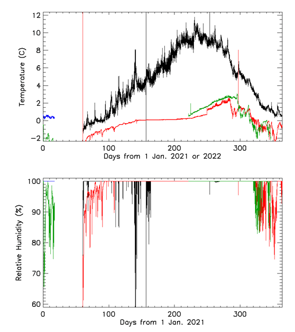
Climate data collected from the mid-cave section of Bonito Flow Ice Cave, 2021–2022, showing air temperature, in degrees Celsius (C) (top), and relative humidity, in percent (bottom). Data collection for the ceiling (location 6, fig. 2 and table 1) is black (2021) and blue (2022). Data collection for the floor (location 5, fig. 2 and table 1) is red (2021) and green (2022).
Back of the Cave Data
The back section of the cave is separated from the mid-cave section as shown on figure 2. Climate data for this part of the cave are shown on figure 13.
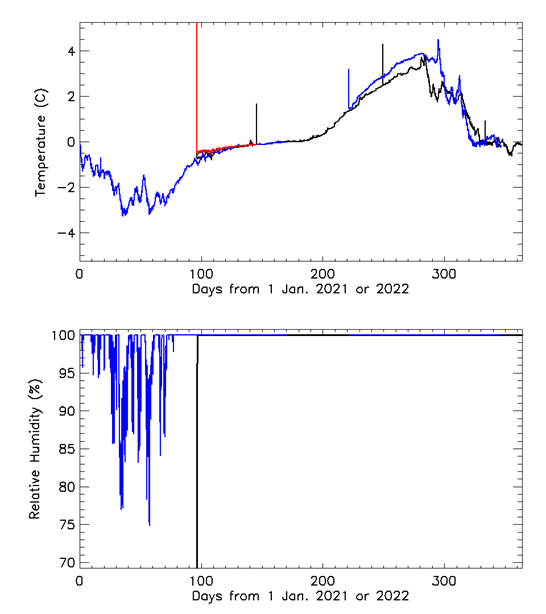
Climate data collected from the back section of Bonito Flow Ice Cave, 2021–2022, showing air temperature, in degrees Celsius (C) (top), and relative humidity, in percent (bottom). Data collection for the T-intersection (location 7, fig. 2 and table 1) is black (2021) and blue (2022). Data collection for the back of the cave (location 8, fig. 2 and table 1) is red. Unfortunately, the sensor that was placed in the back of the cave only worked for a few months. The humidity component of the sensor never operated successfully. However, the back sensor provided sufficient temperature data to show that the entire back passage was close to the same temperature measured at the T-intersection.
Summary
Climate sensors for measuring air temperature, relative humidity, and barometric pressure were distributed throughout Sunset Crater Bonito Flow Ice Cave for 2021–2022, with a focus on a large ice puddle present on the cave floor during the winter months. Air temperatures on the cave floor often showed decreases that correspond to times when the outside air temperature was below the cave air temperature, indicating the flow of colder air into the cave. Cave air was saturated for most of the year. An air temperature gradient existed between the cave floor and ceiling. This ceiling-to-floor temperature gradient was greatest during the summer.
Sunset Crater Bonito Flow Ice Cave may still be an ice cave, but additional monitoring and analysis are needed. The visible presence of ice at the ice puddle location occurred for about 11 of 12 months in 2021–2022, but perennial ice may still exist just below the rocky cave floor. Floor temperatures never rose above a few degrees Celsius and quickly returned to freezing once cold air from the surface flowed into the cave again.
Acknowledgments
The authors thank the staff of the National Park Service Sunset Crater National Monument and the Hopi and Zuni tribes for permitting this research to occur.
Any use of trade, firm, or product names is for descriptive purposes only and does not imply endorsement by the U.S. Government.
References Cited
Cushing, G.E., Titus, T.N., Gullikson, A.L., and Williams, K.E., 2024, Ice cave climate data and frost imagery at Sunset Crater, AZ—02 March 2021 to 13 December 2022: U.S. Geological Survey data release, https://doi.org/10.5066/P9ICPC1M.
Cushing, G., Titus, T.N., Williams, K.E., Gullikson, A.L., and Vaughan, G.R., 2023, Subsurface temperature profiles, imagery, and meteorological data at a Sunset Crater cinder field—March 2021 to May 2022: U.S. Geological Survey data release, https://doi.org/10.5066/P9ICDQUF.
Stoffle, Richard, and Van Vlack, Kathleen, 2022, Talking with a volcano—Native American perspectives on the eruption of Sunset Crater, Arizona: Land, v. 11, no. 2, p. 196. [Also available at https://doi.org/10.3390/land11020196.]
Williams, K.E., and McKay, C., 2015, Comparing flow-through and static ice cave models for Shoshone Ice Cave: International Journal of Speleology, v. 44, issue 2, p. 115–123, https://digitalcommons.usf.edu/ijs/vol44/iss2/1.
Modern Cave Monitoring Informs Interpretations of Past Climate Change: Applications to Titan Cave, Wyoming
Abstract
Monitoring of cave environments is an essential process for deciphering records of past climate change preserved in the geochemical composition of speleothems or mineral cave deposits. This study presents data from a multiyear monitoring effort in Titan Cave, Wyoming, a site of interest due to the abundance of speleothems suitable for paleoclimate reconstruction. Titan Cave exhibits annual cave air temperature fluctuations of less than 0.4 degree Celsius, along with consistent relative humidity, drip rate, and partial pressure of carbon dioxide (pCO2) throughout the year. Small variations in drip rate were noted to be associated with multiseasonal to multiannual regional precipitation trends, such as the widespread western United States drought that lasted from fall 2020 through spring 2022. Stable isotope measurements from drip water (del hydrogen-2 or deuterium [δ2H], del oxygen-18 [δ18O]) are also relatively constant throughout the year and across different drip sites in the cave, varying by only 2 per mil (‰) in δ2H and less than 0.4‰ in δ18O. However, stable isotopes (δ18O, del carbon-13 [δ13C]) measured in modern calcite grown on artificial substrates vary spatially and temporally within the cave.
In the Pisa Room of Titan Cave, modern calcite collected from drip sites in the center of the room is more negative in both δ18O and δ13C than modern calcite collected from drip sites along the room’s wall, suggesting differential water flow paths and (or) in-cave disequilibrium effects. The middle of the Pisa Room was identified as the location best suited for future speleothem paleoclimate reconstruction due to the high density of speleothem growth and calcite δ18O values closer to equilibrium than in other Pisa Room locations. Based on the documented stability of the cave environment and the relative lack of high-resolution paleoclimate data from this region of the northern Rocky Mountains, Titan Cave was found to be a favorable cave for the development of speleothem paleoclimate records.
Introduction
Karst environments hold great potential for preserving records of past terrestrial climate change. Speleothems, or mineral deposits formed in caves over time, can be dated at high precision and preserve a number of climatic signals in their geochemical makeup, revealing aspects of past climate during the speleothem’s growth (Lachniet and others, 2014; Wong and Breecker, 2015; Oster and Kelley, 2016). Speleothems provide the opportunity to reconstruct long-term terrestrial climate change, extending records of past precipitation variability beyond the instrumental and tree ring records (Cheng and others, 2013; Wendt and others, 2018). Geochemical proxies such as ratios of the stable isotopes of oxygen (δ18O) and carbon (δ13C) in the speleothem mineral structure can provide information about past climate variations above a cave. Oxygen isotopes have commonly been used to reconstruct past changes in the δ18O of precipitation, recording shifts in precipitation intensity, seasonality, temperature, and moisture source region (Bar-Matthews and others, 1997; Tremaine and others, 2011). Carbon isotope ratios are reflective of past shifts in soil respiration, vegetation above the cave, water-rock interactions, prior calcite precipitation, and degassing (Fohlmeister and others, 2020). In many environments, changes in speleothem δ13C occur as the result of water availability above the cave, effectively recording wetter vs. drier climate conditions over time (Oster and others, 2020).
Although common climatic and environmental controls on proxies have been documented across landscapes and ecosystems, each cave environment is unique and requires intensive study to effectively translate speleothem geochemical data into useful records of past climate change. Rigorous cave monitoring approaches have proven to be an effective method for understanding location-specific karst processes influencing drip water and speleothem geochemistry (Druhan and others, 2021; Oster and others, 2012, 2021; Sekhon, 2021). These modern monitoring approaches focus on collecting and analyzing cave drip water and calcite precipitated on artificial substrates such as glass plates in the cave, along with recording changes in cave temperature, pCO2, humidity, and drip rate.
In this study, a comprehensive, multi-year dataset is presented that includes measurements of cave temperature, pCO2, relative humidity, drip rate, and water and modern calcite stable isotope compositions from Titan Cave (TC), in northern Wyoming. Titan Cave is the first known cave to be monitored in the northern Rocky Mountains and hosts numerous speleothems dated to significant climatic intervals in Earth’s recent past, including the Holocene and Last Interglacial Period. Titan Cave also sits in a region of the Rockies which lacks high-resolution paleoclimate data beyond the tree ring record (Pederson and others, 2011), despite the importance of this information for better understanding long-term climate variability and drought. Results from this study indicate that speleothems from TC are suitable for reconstructing long-term paleoclimate trends due to limited cave ventilation and minimal changes in cave microclimate and drip rate on seasonal timescales. Lastly, intra-cave variations in drip water and modern calcite geochemistry were noted that are anticipated will be present in speleothem paleoclimate reconstructions from TC.
Methods
Site Description
Titan Cave is a wild cave located in northern Wyoming near the border with Montana (fig. 1A). The cave is managed by the Bureau of Land Management (BLM) specifically for scientific research, and the only known previous study at this site consisted of preliminary radon testing (unpublished). The cave is located in the Bighorn River area and is less than 1 kilometer (km) from Natural Trap Cave, a significant paleontological site. Natural Trap Cave hosts a well-documented fossil record spanning the last glacial cycle (Kohn and McKay, 2010, 2012; Meachen and others, 2016), but no speleothem records of past climate change. Titan Cave is situated in the upper section of the Mississippian-age Madison Limestone, which consists of gray limestone and red siltstone paleokarst-breccia and ranges from 330 to 900 feet thick in this region (Sandberg and Klapper, 1967). The entrance to Titan Cave (TC), at 1,427 meters in elevation, sits in a small depression in the Tensleep Sandstone of the overlying Amsden Formation.
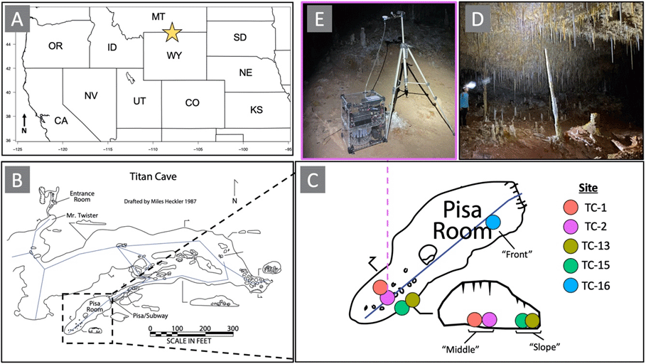
Location map of Titan Cave and inset maps to show drip site location and details. Counterclockwise, from top left: A, Location map of Titan Cave (yellow star), located on the western side of the Bighorn Mountain Range in north-central Wyoming; B, Titan Cave map with key locations marked; C, Zoomed-in map and cross section of the Pisa Room, with drip sites TC-1, 2, 13, 15, and 16 marked; D, Image of the Pisa Room in Titan Cave showing stalactite and stalagmite cave formations; E, Image of the SYP autosampler used to collect drip water at site TC-2. Photographs from Bryce Belanger.
Titan Cave receives both cold-season precipitation (predominantly snow) and shoulder season/summer precipitation from convective storms. Moisture in this region is sourced from air masses originating in the Arctic, the Gulf of Mexico, and the Pacific Ocean (Bryson and Hare, 1974). However, high elevation regions can experience significantly different climatologies compared to lower elevation areas. For example, precipitation at high elevation in the Rocky Mountains is generally dominated by Pacific-sourced winter westerly storm systems (Sjostrom and others, 2006), whereas lower elevation areas may receive greater fractions of summertime precipitation due to the influence of the North American Monsoon (Despain, 1987). Precipitation data from Deaver, WY, about 30 kilometers from TC at a similar elevation, indicate that winter snowfall and summer rainfall equally contribute to the annual precipitation budget in this region (Applied Climate Information System, 2024).
Sample collection and cave monitoring at TC takes place in the Pisa Room, roughly 300 meters from the cave entrance (fig. 1B). Because of the geometry of the cave, the Pisa Room is poorly ventilated and sits beneath an estimated 25–50 meters of overlying host rock. The Pisa Room is characterized by thousands of active and dormant speleothem formations (primarily stalactites and stalagmites), ranging from centimeters to over 3 meters in length (fig. 1D). At present day, the cave itself is mostly dry with limited actively dripping sites.
Cave Monitoring Overview and Sample Collection
Active cave monitoring at TC has been ongoing since September 2019. Visits to the cave have occurred on a biannual basis, usually in the fall and spring. A 2-year hiatus in visitation occurred due to the COVID pandemic between September 2019 and September 2021. Within the Pisa Room, air temperature and humidity were logged continuously from May to October 2022 using an Onset HOBO InTemp Data Logger. The data logger was relaunched in 2023 but data have not been retrieved as of April 2024. Drip rate is also logged continuously at multiple sites using Driptych Stalagmate acoustic drip loggers. Monitoring efforts have been focused on the section of the Pisa Room farthest from the cave entrance at five active drip sites, TC-1, TC-2, TC-13, TC-15, and TC-16 (fig. 1C). These sites were selected due to the presence of modern drip water and proximity to stalagmites recovered for paleoclimate reconstruction.
Stalagmate drip loggers were active at site TC-1 from November 2019 to January 2023, site TC-2 from September 2021 to May 2022, and site TC-15 from September 2021 to October 2023. Cave air pCO2 was measured in the Pisa Room using a Vaisala CARBOCAP GMP252 CO2 probe or an AZ Instrument Corp. 77535AZ EB handheld pCO2 meter during each visit to the cave.
Drip water was sampled from TC using two methods. First, water was sampled instantaneously from multiple drip sites during biannual visits to the cave. Limited water availability and long drip intervals have restricted water sampling via this method. The few samples retrieved (n=6) via instantaneous sampling were collected for analysis of δ18O and δ2H in pre-cleaned 2-milliliter (ml) vials with limited headspace. In an effort to expand drip water sampling efforts at TC, a Waikato Scientific SYP water autosampler was installed in the Pisa Room at site TC-2 in late May 2022 and has been collecting water at 4-day intervals (fig. 1E). The 10-ml vials fill in approximately 12 hours, providing adequate water for δ18O, δ2H, and trace element analyses at sub-weekly resolution. In October 2023, freshly fallen snow was collected for stable isotope analysis in pre-cleaned 15-ml Falcon tubes. All water samples were kept refrigerated until analysis.
Water Sample Analysis
Drip water (n = 125) and snow (n=2) samples were analyzed on a Picarro L2130-i Isotopic Water Analyzer at Vanderbilt University. Each measurement consisted of four preparatory injections to minimize memory effects, and four measured injections. Samples were measured at least twice and corrected using external U.S. Geological Survey (USGS) reference water standards through the USGS LIMS for Lasers data reduction scheme (Coplen, 1998). Data are presented in per mil (‰) relative to the Vienna Standard Mean Ocean Water (VSMOW) international standard. Typical precision of stable isotope measurements is about 0.02‰ for oxygen and about 0.1‰ for hydrogen (1σ).
Modern Calcite Collection and Analysis
Modern calcite was collected at sites TC-1, TC-2, TC-13, TC-15, and TC-16 in the Pisa Room. Glass plates, frosted via abrasion on a polishing wheel at 70-micrometer grit size, were carefully placed under each drip site and allowed to accumulate calcite precipitating from drip water between visits to the cave. Following recollection, samples of precipitated calcite were gently scraped from the frosted glass plates using a razor blade. The powdered calcium carbonate samples were then analyzed for δ18O and δ13C using a Thermo Finnigan DeltaV Plus isotope ratio mass spectrometer coupled to a Gasbench-II at Vanderbilt University. Carbonate powders were weighed into LabCo exetainers and dried overnight at 50 degrees Celsius (°C). Vials were then flushed with helium for 10 minutes. Anhydrous orthophosphoric acid was added to the vials, and the samples were allowed to react at 70 °C for at least 1 hour. Samples were corrected using in-house standards Thermo Calcite and VU-Coral that are referenced to the international standards IAEA-603 and NBS-18, respectively. Corrections were conducted using the USGS LIMS for Light Stable Isotopes data reduction scheme (Coplen, 1998). Data are presented in per mil (‰) relative to the Vienna PeeDee Belemnite (VPDB) international standard. Typical precision of stable isotope measurements is about 0.08‰ for oxygen and about 0.05‰ (1σ) for carbon.
Results
Cave Air Temperature, Relative Humidity, and pCO2
Cave air temperature remained nearly constant in the Pisa Room from May 2022 until October 2022, averaging 9.59 °C with a standard deviation of plus or minus 0.05 °C. July was the warmest 30-day interval during the monitoring period (9.63 °C) and September 13th to October 13th was the coldest interval (9.55 °C). Relative humidity was close to 100 percent (%) and thus variations were not well-captured by the data logger. Average Pisa Room cave air pCO2 was 577 parts per million (ppm) with approximately 100 ppm variability between Spring and Fall (table 1).
Drip Rate
Drip rate at all monitored sites in the Pisa Room is consistently slow, rarely reaching rates faster than one drip every 2 minutes (fig. 2). Site TC-15 has the slowest drip rate, averaging 0.12 drips per minute (dpm) during the monitoring period, which spans from September 2021 until October 2023, with a short hiatus due to a dead drip logger battery. TC-15 drip rate is nearly constant, excluding a slight positive trend toward faster drip rates from June through August 2023. During the overlapping period in the two records, trends in drip rates are nearly identical at sites TC-1 and TC-2, however, mean drip rate is roughly twice as fast at TC-1 (0.47 dpm) compared to TC-2 (0.20 dpm) (fig. 2). Drip rates at TC-1 and TC-2 show high correlation (Pearson’s R = 0.91, p <0.0005), displaying nearly synchronous changes on hourly to daily timescales. This strong coherence is unsurprising as the sites are only about 2 meters apart. TC-1 drip rate declines steadily during the monitoring period, decreasing by roughly 0.05 dpm per year from 2019 to 2023. TC-1 drip rate begins decreasing less rapidly in Summer 2022, synchronous with increasing summer rainfall in Deaver, WY (fig. 2).
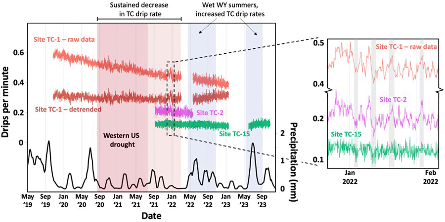
Titan Cave (TC) drip logger data and Deaver, WY weather data (Western Regional Climate Center, 2024) from May 2019 to December 2023. From top to bottom, TC-1 drip logger raw data (red), TC-1 drip logger data detrended using detrend function in R (maroon), TC-2 drip logger data (magenta), TC-15 drip logger data (green), and 15-point moving average of mean daily precipitation (in mm) over previous 30-day period in Deaver, WY (black). Western US drought selected based on Seager and others (2022) is highlighted by the dark red vertical bar labelled “Western US drought.” Lighter red vertical bar demarcates extended dry conditions at TC. Blue vertical bars demarcate rainier summers at TC following drought conditions. Inset graph at right shows drip logger data from 12/20/21 to 2/8/22. Note break in y-axis. Gray bars highlight consistencies in drip rate response across all three sites.
Water Isotopes
Pisa Room drip water δ18O values range from −20.26 per mil (‰) to −19.9‰, and δ2H values range from −158.94‰ to −157.07‰ (fig. 3). Water collected for δ18O at 4-day intervals using the autosampler at site TC-2 ranges between only −20.26‰ and −20.16‰ from May 2022 to October 2023. Considering the analytical uncertainty of 0.02% (1σ), the variability in site TC-2 drip water δ18O appears to be extremely limited (fig. 4). Limited inter-site δ18O variability within the Pisa Room was also noted. Drip water δ18O collected instantaneously at sites TC-1 and TC-15 in October 2023 are identical within analytical uncertainty (−20.06‰ and −20.08‰), and instantaneously collected drip water from TC-1 in September 2021 is also similar (−20.02‰). Drip water collected near the cave entrance (site MT drip on fig. 3) in September 2021 and October 2022 is notably more enriched in 18O, with values of −18.19‰ and −17.75‰ measured, respectively. Two snow samples collected from above TC in October 2023 have an average δ18O value of −23.90‰ and a δ2H value of −175.54‰.
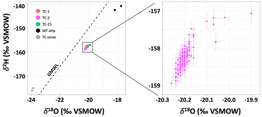
All Titan Cave water stable isotope data. “TC snow” samples (gray) were collected from fresh snow directly above the Pisa Room on 10/26/23. “MT drip” samples (black) were collected from the Mr. Twister section of the cave (see figure 1B) on 9/15/21 and 10/13/22. Site TC-1 samples (red) were collected on 9/15/21, 6/18/22, and 10/26/23. Site TC-15 samples (green) were collected on 6/18/22 and 10/26/23. TC-2 samples (magenta) were collected using the SYP autosampler from 5/31/22 to 10/26/23 at 4-day intervals. Representative error bars for repeat analyses (0.1 per mil [‰] for δ2H and 0.02‰ for δ18O [both 1σ]) are shown. Error bars are smaller than symbols in main figure. Dashed line represents global meteoric water line (GMWL) with slope=8 and y-intercept=10.
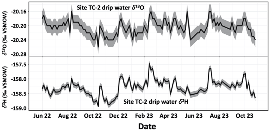
Stable oxygen isotope (δ18O) timeseries measured from site TC-2 drip waters in the Pisa Room of Titan Cave. Waters were collected at 4-day intervals (over about 12 hours) from 5/31/22 to 10/26/23, using the SYP water autosampler. Representative error bars (1σ) for repeat analyses (plus or minus 0.02‰) are shown.
Modern Calcite Stable Isotopes
Modern plate calcite δ13C values range from −6.11‰ to 0.65‰ and δ18O values range from −17.33‰ to −15.43‰ (figs. 5 and 6; table 2). Within the Pisa Room, systematic variations in modern calcite δ13C and δ18O were noted, based on drip site location (fig. 5), in addition to changes with time (fig. 6). Sites TC-1 and TC-2, located in the center of the Pisa Room, record more negative calcite δ13C and δ18O values compared to sites TC-13 and TC-15 which sit closer to the cave wall.
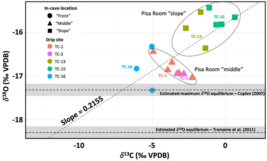
Stable carbon (δ13C) and oxygen (δ18O) isotope data collected from calcium carbonate formed on glass plates in the Pisa Room of Titan Cave. Sites TC-1 and TC-2 are located in the middle of the Pisa Room under a high cave ceiling (see figure 1C), sites TC-13 and TC-15 sit against the room wall under a low cave ceiling, and site TC-16 is in a separate part of the room under a high ceiling. Linear regression of the data yields a slope of 0.2155. Estimated equilibrium calculated using Tremaine and others (2011) and Coplen (2007) as described in text. See table 2 for raw data and timing of plate calcite collection.
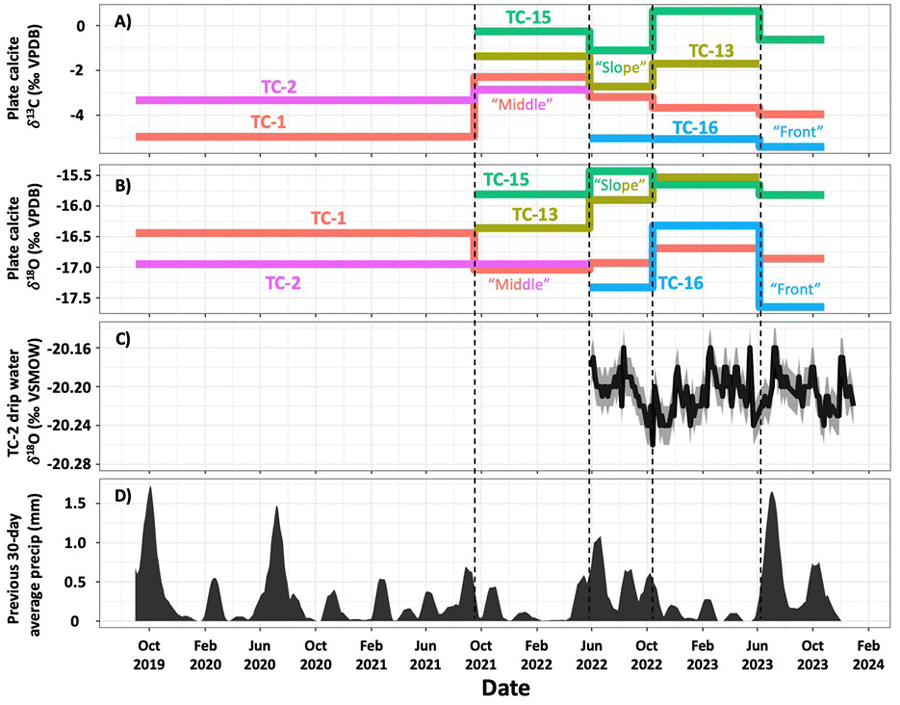
Pisa Room stable isotope data and Deaver, WY weather data (Western Regional Climate Center, 2024). A) Stable carbon (δ13C) and B) oxygen (δ18O) isotope timeseries from farmed calcium carbonate precipitated on glass plates at sites TC-1, 2, 13, 15, and 16. C) Site TC-2 drip water stable isotope (δ18O) timeseries (same as fig. 4). D) 15-point moving average of mean daily precipitation (in mm) over previous 30-day period in Deaver, WY. Dashed lines mark when glass plates were collected and replaced.
Table 2.
Titan Cave plate calcite stable isotope data.[δ13C, del carbon-13; δ18O, del oxygen-18; ‰ VPDB, per mil Vienna PeeDee Belemnite]
Discussion
The suite of monitoring data collected from Titan Cave across multiple years allows for the systematic and cave-specific interpretation of geochemical variability recorded in drip water and modern plate calcite at this site. In this section, individual monitoring datasets from TC are discussed. These data are then summarized and synthesized as it relates to interpretations of past climate change in the Bighorn region as recorded via TC speleothems.
Cave Air
Titan Cave air temperature, pCO2, and humidity are remarkably constant throughout the year and over the duration of the monitoring period. In the Pisa Room, cave air temperature varies by less than 0.1 °C seasonally, suggesting limited exchange with surface air and restricted air flow to this room in TC where speleothem growth is occurring. Our interpretation of poor ventilation to the Pisa Room is further supported by relative humidity measurements, which remain close to 100% and vary by less than 1% throughout the monitoring period. Cave air pCO2 is also relatively constant and remains about 200 ppm greater than atmospheric levels throughout the year, further supporting our interpretation of limited surface air ventilation to the Pisa Room.
Drip Rate
Drip rates in the Pisa Room show muted changes in response to weather events and seasonal shifts above the cave. In contrast to other caves in the United States (Oster and others, 2012; Sekhon, 2021), TC drip rates are relatively insensitive to precipitation events and spring snowmelt. Instead, TC drip rates increase or decrease by only 10–20% on seasonal to multi-year timescales as a reflection of longer-term variations in precipitation amount.
The most notable trend in TC drip rate data is the sustained decrease in site TC-1 drip rate from fall 2019 through winter 2023. This trend is relatively constant and uninterrupted by precipitation seasonality or individual rainfall or snowmelt events. Overall, this trend is interpreted to reflect the drought conditions sustained in north-central Wyoming from fall 2020 through spring 2022. Well-documented drought in the western US (including Wyoming) occurred from summer 2020 to spring 2021 (Seager and others, 2022). Decreasing drip rates at site TC-1 during this interval suggest that multi-seasonal to multi-annual precipitation trends above TC have the strongest control on drip rate at this location. Notably, an examination of detrended TC-1 drip rate data shows a positive trend beginning in summer 2022, the same time when a rainy summer in Wyoming led to the amelioration of drought conditions in the region (fig. 2). Site TC-15 also records a small (approximately 5%) uptick in average drip rate during the even wetter summer of 2023.
A potential inconsistency in these interpretations is the lack of a drip rate change at site TC-1 coincident with rainy conditions in summer 2020 (fig. 2). The absence of a drip rate response to this event further highlights the smoothing of climate signals being transferred to the cave environment at TC. However, it may also demonstrate the importance of summer evaporation on TC drip rate, as average daily pan evaporation in Powell, WY (about 50 kilometers southwest of TC) was 70% higher in summer 2020 (no drip rate increase) compared to summer 2022 when detrended TC-1 drip rate data show a positive trend (Western Regional Climate Center, 2024). Titan cave drip rates also increase slightly during summer 2023, however, pan evaporation data are not available for this period. Overall, TC drip rate data suggest that multi-seasonal to multi-year precipitation trends are relayed to the cave environment, while the signal of short-term rainfall and snowmelt events are smoothed by water mixing and slow infiltration times in the karst above TC.
Small fluctuations in drip rate on hourly to daily timescales are nearly identical at sites TC-1 and TC-2. When comparing daily averaged dpm from sites TC-1 and TC-2, a Pearson’s R value of 0.91 (p <0.0005) is calculated. During their overlapping period of record from September 2021 to March 2022, drip rates at both sites varied by a maximum of only 0.1 dpm. However, these slight variations in drip rate are mirrored at both sites, suggesting a common control on water delivery. Sites TC-1 and TC-2 are separated by only 2 meters in the Pisa Room, therefore this common control on drip rate could be linked to a shared flow path between the sites. Drip water stable isotope values are nearly identical between the two sites, providing further support for a shared flow path to TC-1 and TC-2. Site TC-15, which is separated from TC-1 and TC-2 by roughly 10 meters, also shows similar drip rate trends. When comparing daily averaged dpm from sites TC-1 and TC-15, a Pearson’s R value of 0.83 (p <0.0005) is calculated, and a value of 0.86 (p <0.0005) is calculated when comparing TC-2 and TC-15. Both correlations are strong although weaker than between TC-1 and TC-2. This is possibly due to extremely slow drip rates at TC-15 (less than 0.15 dpm) and limited drip rate variability, in addition to the physical distance between the sites.
Water Isotopes
Water isotopes in cave drip water can reflect numerous processes, both above and within the karst environment. Due to slow drip rates within TC and the Pisa Room, the majority of drip water collection occurred at site TC-2 using the SYP autosampler. As with drip rate, there is little variation in drip water δ2H and δ18O at TC-2 during the monitoring period (figs. 3 and 4). In both 2022 and 2023, drip water δ2H and δ18O values increased in July and August by about 0.5‰ and about 0.05‰ respectively, before falling steadily during October (fig. 4). This pattern suggests a slight seasonal control on drip water isotopic composition. Increasingly negative δ2H and δ18O during the fall could reflect the delivery of moisture sourced from more northern regions during the shift from summer to winter precipitation regimes (Oster and others, 2020). However, this theory does not explain the return to more positive isotopic values during December 2022. An extended period of drip water collection at TC-2 is necessary to elucidate multi-year trends in water isotope composition. Because of the limited variability of drip water δ2H and δ18O on seasonal timescales, multi-year trends in precipitation are possibly responsible for isotopic shifts recorded in TC speleothems. As with TC drip rate, event to seasonal-scale variability in precipitation δ2H and δ18O above TC is not transferred through the epikarst to the Pisa Room.
A small number of instantaneously collected TC drip waters provide important details regarding intra-cave variations in δ2H and δ18O values. Within the Pisa Room, sites TC-1, TC-2, and TC-15 all record similar δ18O values between −20.25‰ and −19.9‰. Limited variability in drip water δ18O between sites provides further evidence that delivery of water to sites throughout the Pisa Room is controlled by shared karst processes, and therefore will respond similarly to climatic and environmental changes. Because of limited systematic departures from the global meteoric water line, evaporation of water prior to dripping is likely not influencing drip water stable isotope composition in the Pisa Room (fig. 3).
Modern Calcite Stable Isotopes
Stable oxygen and carbon isotopes in speleothems (and modern calcite) are influenced by various processes acting over multiple timescales. Possible controls on long-term δ13C variability include the ratio of C3 to C4 vegetation above the cave (Burns and others, 2016; Fohlmeister and others, 2020), temperature as it relates to soil respiration (Fohlmeister and others, 2020), and atmospheric CO2 concentrations at the time of speleothem growth (Breecker, 2017). On shorter timescales, changes in water supply and variations in soil respiration, CO2 degassing, and prior calcite precipitation likely play a larger role in dictating seasonal to multi-year δ13C fluctuations at TC (Ersek and others, 2012, Oster and others, 2012, 2020).
Speleothem δ18O reflects the δ18O of precipitation above the cave site, potentially modified by evaporation and water mixing in the karst, and changes during calcite precipitation via non-equilibrium processes and temperature-dependent fractionation in the cave (Baker and others, 2019). Coeval speleothem records from the same cave do not always display the same trends or mean values, demonstrating the possibility for control on speleothem δ18O by flow path variability (Treble and others, 2022) and in-cave disequilibrium processes (Mickler and others, 2004, 2006). Progressive CO2 degassing before and during calcite precipitation in the cave leads to positive excursions in δ13C and δ18O due to the preferential loss of 12C and 16O into the gas phase (Dreybrodt and Scholz, 2011). Therefore, when a positive linear relationship is observed between δ13C and δ18O, it can indicate disequilibrium processes (Hendy, 1971; Mickler and others, 2004, 2006). The slope of this linear relationship can vary due to the degree of carbon isotope exchange between dissolved inorganic carbon (DIC) in the drip water and CO2 in the cave atmosphere (Parvez and others, 2024).
At Titan Cave, plate calcite δ13C and δ18O values are variable in both space and time (figs. 5 and 6). Most notably, drip sites in the middle of the Pisa Room (TC-1, TC-2) are consistently more negative in δ13C by about 2‰ and δ18O by about 1.5‰ compared to the sites located near the room’s wall (TC-13, TC-15). Because of the lack of consistent drip water sampling across sites, a karst (flow path hydrology) control on this observed isotopic variability cannot be ruled out. In this case, we would expect plate calcite at sites TC-1 and TC-2, which display more negative isotopic ratios, to receive proportionally larger amounts of recharge from snowmelt or isotopically lighter water sources compared to TC-13 and TC-15. Additionally, we would expect less CO2 degassing in the epikarst above TC-1 and TC-2 due to faster/less disrupted water flow. These are both reasonable assumptions given the faster drip rates observed in the center of the Pisa Room that are more responsive to surface precipitation, indicative of more fracture-based flow. This would allow increased recharge during periods of snowmelt (more negative δ18O) and less time for prior calcite precipitation (PCP) in the karst (more negative δ13C). Following the classification scheme of Smart and Friederich (1986) all TC drips are determined to be dominated by seepage (or diffuse) flow due to their low maximum water discharge and low drip rate variability (Baldini and others, 2006; Tremaine and Froelich, 2013; Wong and Breecker, 2015). However, although absolute differences in drip rate and drip variability are small, relative differences in these metrics between drip sites is quite large, suggesting that flow paths to various TC drips may be different despite all falling under the seepage/diffuse flow classification.
If it is assumed that flow paths and drip water δ18O are consistent between sites in the Pisa Room, disequilibrium processes must be invoked to explain intra-cave differences in the isotopic composition of calcite. Calcite formed at all drip sites within the Pisa Room is more positive in δ18O than would be expected at TC based on measured drip water δ18O values (fig. 5). Given a constant Pisa Room temperature (9.59 °C) and average measured drip water δ18O (−20.2‰ VSMOW), the equilibrium relationship of Tremaine and others (2011) predicts speleothem δ18O values of approximately −18.3‰ VPDB, or about 1‰ more negative than any measured TC plate calcite value. Using the most positive δ18O water isotope value (−19.9‰ VSMOW) and lowest temperature (9.46 °C) value, the Tremaine and others (2011) equation still yields an equilibrium δ18O value as low as −18.0‰ VPDB. To determine if equilibrium relationship selection is the source of this offset, the same cave parameters and the equilibrium relationship of Coplen (2007) were employed, which was calculated using a different set of empirical data than Tremaine and others (2011). This equation predicts a calcite δ18O value of −17.4‰ VPDB, which only aligns with calcite δ18O values measured at site TC-16 (fig. 5). This suggests a departure of TC plate, and thus potentially speleothem, calcite to more positive δ18O values due to preferential degassing of 16O during calcite formation at most or all Pisa Room drip sites.
A positive correlation also exists between the measured δ13C and δ18O of TC plate calcite (slope = 0.2155, R2 = 0.46) (fig. 5). This slope falls within the range of slopes reported by Parvez and others (2024) in an investigation of disequilibrium and carbon isotope exchange between cave air CO2 and DIC in the drip water. In this situation, the slower drip rates observed along the walls of the Pisa Room (sites TC-13 and TC-15) would enable increased time for degassing and isotopic exchange prior to calcite precipitation, therefore driving δ13C and δ18O to more positive values. At the center of the cave (sites TC-1 and TC-2), faster drip rates lead to more rapid replenishment of DIC and H2O reservoirs with fresh cave water, thus maintaining more negative isotopic values closer to equilibrium. Plate calcite timeseries data (fig. 6) show that these relationships are consistent through time, as δ13C and δ18O at TC-1 and TC-2 are always more negative than at TC-13 and TC-15, despite variability from one plate collection interval to the next.
On the basis of these observations, it is possible that both karst processes, in-cave degassing, or both, are contributing to the intra-cave variations in plate calcite δ13C and δ18O. Future trips to Titan Cave will focus on collecting drip water from additional sites within the cave to further investigate variability in drip water δ18O.
Implications for Paleoclimate Reconstruction at Titan Cave
Titan Cave monitoring efforts have demonstrated the suitability of TC speleothems for paleoclimate reconstruction. Constant cave temperature, relative humidity, and pCO2 limit opportunities for seasonal biases to arise in TC speleothems. In caves where temperatures and calcite growth rates exhibit large seasonal variations, changes in δ18O may be driven by changes in temperature-dependent equilibrium fractionation instead of recording shifts in hydroclimate (Mickler and others, 2004). Similarly, constant relative humidity limits season-specific changes in the degree of disequilibrium fractionation, influencing calcite δ13C and δ18O. Consistent cave air pCO2 is also important for limiting growth biases, as calcite precipitation is reduced when pCO2 is high (Baldini and others, 2008), and seasonal variations in pCO2 can drive PCP shifts independent of hydroclimate controls (Oster and others, 2012). Elevated pCO2 levels may also drive increased carbon isotope exchange (Skiba and Fohlmeister, 2023). This risk is limited at TC due to consistent pCO2 throughout the year.
Additionally, TC drip rate does not fluctuate seasonally or as a result of event-scale precipitation. Rather, a sustained, multi-year drought resulted in the slow reduction in drip rate at some sites. Drip water collected via the SYP autosampler at 4-day intervals over 16 months records only 0.1‰ variability in δ18O, just beyond the limits of analytical uncertainty. Titan Cave plate calcite also records minimal shifts in isotopic composition, with calcite δ18O and δ13C varying by only 1‰ and 2‰, respectively, at a single drip site (fig. 5). Furthermore, plate calcite δ18O and δ13C do not shift dramatically as the result of seasonal variations or changes in precipitation amount (fig. 6). A −1‰ shift in δ13C at sites TC-1, TC-13, and TC-15 was observed during the relatively wet summer of 2022, possibly reflective of more rapid water infiltration and reduced PCP. These observations indicate that TC speleothems will document time-averaged records of hydroclimate in the Bighorn region.
Analysis of stable isotopes in plate calcite from multiple Pisa Room sites provides critical context for reconstructions of paleoclimate using TC speleothems. Modern calcite data show that variable water flow paths and/or disequilibrium effects may be driving differing degrees of δ18O and δ13C change in the center of the Pisa Room compared to the sides (figs. 5 and 6). These observations provide two key insights when interpreting Pisa Room speleothem records. First, similar offsets between coeval speleothem records may exist in the Pisa Room. If this is the case, it should reflect (1) spatial variability in karst processes, or (2) differential Rayleigh fractionation processes within the cave. If temporal trends in δ18O and δ13C are consistent among stalagmites from different sites within the cave, this should confidently be interpreted to reflect regional hydroclimate change. Second, speleothems growing in the center of the Pisa Room will likely record isotopic values closer to equilibrium compared to those growing along the wall and are thus best suited for paleoclimate reconstruction.
Conclusions
This study presents data from the first known comprehensive, multi-year cave monitoring campaign in the Rocky Mountains in the western conterminous United States. The dataset includes measurements of cave temperature, relative humidity, pCO2, drip rate, and water and modern calcite stable isotope compositions from Titan Cave, Wyoming. Monitoring efforts reveal a remarkably stable cave environment, with consistent cave temperature, humidity, and pCO2 throughout the year. Small fluctuations in drip rate were observed that are consistent with multi-seasonal to annual trends in precipitation, along with slight shifts in drip water and plate calcite stable isotope values on similar timescales. Modern plate calcite δ18O and δ13C values show intra-cave variability along with a systematic trend away from isotopic equilibrium conditions in specific areas of the cave. Thus, the middle of the Pisa Room was identified as the location best suited for future speleothem paleoclimate reconstructions due to the high density of speleothem growth and calcite δ18O values closer to equilibrium than at other Pisa Room locations. Because of the documented stability of the cave environment and abundant suitable stalagmites, Titan Cave was found to be a favorable cave for the development of speleothem proxy records.
Acknowledgments
This work was funded by National Science Foundation Award AGS2102994 to Jessica Oster. The work was also funded by the Geological Society of America Graduate Student Research Grant 13028-21 and the Cave Research Foundation Graduate Research Grant and awarded to Bryce Belanger. The authors acknowledge Aida Zyba and Richard Bradshaw (Vanderbilt University) for assistance in field and lab work. The authors also acknowledge Lisa Marks and Shelby Miller (Bureau of Land Management) for field work assistance, and the agency for access to Titan Cave. Finally, the authors thank reviewers and Christopher Kinsley and Natasha Sekhon for helpful feedback.
References Cited
Applied Climate Information System, 2024, NOAA Regional Climate Centers: SCENIC web page, accessed May 6, 2024, at https://wrcc.dri.edu/csc/scenic/about/.
Baldini, J.U., McDermott, F., Hoffmann, D.L., Richards, D.A., and Clipson, N., 2008, Very high-frequency and seasonal cave atmosphere pCO2 variability—implications for stalagmite growth and oxygen isotope-based paleoclimate records: Earth and Planetary Science Letters, v. 272, issues 1–2, p. 118–129.
Cheng, H., Edwards, R.L., Shen, C.C., Polyak, V.J., Asmerom, Y., Woodhead, J., Hellstrom, J., Wang, Y., Kong, X., Spötl, C., and Wang, X., 2013, Improvements in 230Th dating, 230Th and 234U half-life values, and U–Th isotopic measurements by multi-collector inductively coupled plasma mass spectrometry: Earth and Planetary Science Letters, 371, p. 82–91.
Parvez, Z.A., El-Shenawy, M.I., Lucarelli, J.K., Kim, S.T., Johnson, K.R., Wright, K., Gebregiorgis, D., Montanez, I.P., Wortham, B., Asrat, A., and Reinhardt, E., 2024, Dual carbonate clumped isotope (Δ47-Δ48) measurements constrain different sources of kinetic isotope effects and quasi-equilibrium signatures in cave carbonates: Geochimica et Cosmochimica Acta, v. 366, p. 95–112.
Smart, P.L., and Friederich, H., 1986. Water movement and storage in the unsaturated zone of a maturely karstified carbonate aquifer, Mendip Hills, England, in Proceedings of the Environmental Problems in Karst Terranes and Their Solutions Conference, Bowling Green, KY, October 28–30, 1986: Dublin OH, National Water Well Association, p. 59–87.
Treble, P.C., Baker, A., Abram, N.J., Hellstrom, J.C., Crawford, J., Gagan, M.K., Borsato, A., Griffiths, A.D., Bajo, P., Markowska, M., and Priestley, S.C., 2022, Ubiquitous karst hydrological control on speleothem oxygen isotope variability in a global study: Communications Earth & Environment, v. 3, issue 1, p. 29.
Western Regional Climate Center, 2024, Western Regional Climate Center web page, accessed May 2024, at https://wrcc.dri.edu/.
Planetary Caves From Mercury to Pluto
Abstract
On Earth, caves are unique environments at the intersection of geology, climate, and biology. Given that the same terrestrial speleogenetic processes exist throughout the solar system, it would be surprising if caves beyond Earth did not exist. Thousands of potential cave entrances (or subsurface access points) have been identified from Earth’s Moon to Pluto’s moon, Charon. To date, our most comprehensive knowledge of these potential subsurface access points is for the Moon, Mars, and Titan, which collectively contain more than 20,000 features. Missions are either ongoing or planned for these three planetary bodies. One of these missions may ultimately detect a cave and potentially confirm it contains a laterally trending passage.
Introduction
There are multiple definitions of caves in the scientific literature, but for purposes of this abstract caves are defined as a subsurface void that is potentially accessible from the surface. On Earth, caves are unique subsurface environments at the intersection of geology, climate, and biology. The subterranean realm contains critically important habitats for a panoply of lifeforms including bats (Furey and Racey, 2016), subterranean-adapted fauna (Howarth and Wynne, 2022; Deharveng and others, 2024), relict plant species (Wynne and others, 2014; Monro and others, 2018; Ren and others, 2021), and microbes (Tomczyk-Żak and Zielenkiewicz, 2016; Hershey and Barton, 2018). Caves are also time capsules of the past, enabling researchers to reconstruct past geological processes and environmental histories (Wong and Breecker, 2015; Comas-Bru and others, 2019), as well as serving as treasure troves of paleontological (Jass and George, 2010; Schubert and Mead 2012; Berger and others, 2015; Douka and others, 2019) and archaeological (Moyes, 2012; Sponsel, 2015; Brady and Prufer, 2021) materials.
Given that the same fundamental speleogenetic processes on Earth exist throughout the solar system, it would be surprising if caves beyond Earth did not exist. Scientific speculation about caves on the Moon date back to 1966 (Heacock and others, 1966; Halliday, 1966), when images of rilles were suggested to be surface expressions of lava tubes. These papers were followed by additional studies on lunar lava tube formation processes (Oberbeck and others, 1969; Greeley, 1971), and were later expanded to include Mars using Viking data (Carr and others, 1977).
In 2007, with the advent of high spatial resolution imaging of the surface of Mars, seven deep cylindrical pits were discovered in the volcanic region of Arsia Mons (Cushing and others, 2007). Although these features have yet to be confirmed as actual cave entrances (providing access to horizontally extended subsurface voids), they did mark a notable milestone in planetary cave science.
The same year, 2007, was also the advent of a series of planetary cave workshops and conferences that brought together an interdisciplinary and international group of scientists and engineers with the common goal of studying caves on Earth and beyond. The first workshop was the Lava Tubes: Earth–Moon–Mars workshop convened at El Malpais National Monument, Grants, NM. A list of all workshops and conferences since 2007 are provided in table 1.
Table 1.
Planetary cave workshops and conferences.| Conference1 | Date | Location | Website | Eos Articles |
|---|---|---|---|---|
| Lava Tubes | SEP. 2007 | Grants, NM | None | None |
| 1st IPCW | OCT. 2011 | Carlsbad, NM | https://www.lpi.usra.edu/meetings/caves2011/ | Titus and Boston (2012) |
| 2nd IPCC | OCT. 2015 | Flagstaff, AZ | https://www.hou.usra.edu/meetings/2ndcaves2015/ | Wynne and others (2016) |
| 3rd IPCC | FEB. 2020 | San Antonio, TX | https://www.hou.usra.edu/meetings/3rdcaves2020/ | Titus and others (2020) |
| 4th IPCC | MAY 2023 | Lanzarote, Spain | https://www.hou.usra.edu/meetings/4thcaves2023/ | None |
Planetary Cave Goals and Objectives
In the last Planetary Science Decadal Survey, a white paper focusing on planetary caves (Titus, Wynne, Boston, and others, 2021) proposed a series of goals and objectives for this emerging sub-discipline (table 2). Although these goals and objectives will likely be updated during the next International Planetary Cave Conference, Titus, Wynne, Malaska, and others (2021) provided a viable framework for the path forward. In addition, Wynne, Mylroie, Titus, and others (2022) conducted a survey of the planetary cave research and exploration community to identify the highest priority planetary cave science and engineering questions that should be addressed over the next few decades. We aligned the existing objectives with the appropriate top 15 questions; many of the questions are technology- and capability-based, as opposed to purely focused on science (table 2). This suggests that the expansion of the goals and objectives document should not only include science investigations, but also technology development and testing activities.
Table 2.
Planetary cave research goals and objectives.[Table modified from Titus, Wynne, Boston, and others, 2021. TRL, Technology Readiness Level]
We provide the question number (Q), the rank of each question, the section heading from the paper, and where appropriate, additional details concerning the question. Refer to Wynne, Titus, Agha-Mohammadi, and others (2022) for more information.
Planetary Cave Formation Processes
Our understanding of cave formation processes starts with an understanding of terrestrial caves and their associated speleogenetic processes that initiate and drive their modification. Table 3 describes cave formation processes—most of which occur on Earth. The first step in identifying where caves may exist beyond Earth begins with low-resolution imaging that shows the morphologies of various planetary landscapes are consistent with cave formation processes. As such, this represents the key starting point for any planetary cave inventory.
Table 3.
Classification of cave-forming types and processes, and potential planetary locations for caves.[Table modified from Boston, 2004; Titus and others, 2020; Wynne, Mylroie, Titus, and others, 2022. ?, unknown or none identified; N/A, not applicable]
Cave-forming type proposed by Boston (2004), but not identified by Wynne, Mylroie, Titus, and others (2022). Some of the Boston (2004) types partially overlap with Wynne, Mylroie, Titus, and others (2022) types.
Exploration Framework: Identify, Characterize, Explore!
To identify potential caves, landscape mapping and characterization images must be assessed to determine whether speleogenetic processes may exist on a given planetary body. This can be accomplished using low-to-medium spatial resolution optical or infrared imagery for bodies with no or relatively transparent atmospheres, and with radar for those bodies with thicker, partially opaque atmospheres. For most rocky and icy planetary bodies, we are at this stage of knowledge. As higher spatial resolution imagery becomes available, as is currently the case for the Moon and Mars, these data could be used to identify potential cave entrances, partially depressed segments, or other surface indicators.
Characterization is the next step in the proposed framework (table 4 and fig. 1). This can range from imaging confirmation that a potential cave entrance visually connects to a lateral subsurface passage to the use of methods, including geophysical surface remote sensing techniques (for example, ground penetrating radar (GPR), electrical resistivity, seismic tomography, or gravity measurements) to map the extent of the feature.
Exploration is the final phase and ranges from robotic entry and examination of the interior of the cave to long-term monitoring of climatic, seismic, and radiation environments. Ultimately, this will include human exploration and use of caves beyond Earth (Boston, 2000, 2010).
Table 4.
Exploration and cave inventory framework.[Refer to figure 1. Table modified from Titus, Wynne, Boston, and others, 2021]
Solar System Inventory
Up to this point, the word “cave” has been used to refer to a subsurface void that is potentially accessible from the surface. Wynne, Mylroie, Titus, and others (2022) introduced the term subsurface access points (or SAPs) (fig. 1). The authors defined an SAP as an opening on the surface of a planetary body detectable by remote sensing; this definition is more compatible with the current remote stage of planetary cave research and exploration. This term captures features ranging from deep fissures to atypical pit craters, which may not be immediately perceivable as a fully developed cave but may have undetected lateral passage associated with it.
Cave formation processes exist across the solar system from Mercury to Pluto (Wynne, Mylroie, Titus, and others, 2022). Thousands of potential cave entrances (or SAPs) have been identified from as close as our own Moon to as far away as Pluto’s moon, Charon. To date, our most comprehensive knowledge of SAPs is for the Moon, Mars, and Titan, which support 221, 1,062, and 21,706 features, respectively (fig. 1 and table 5).
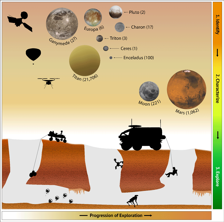
Progression of exploration for identifying, characterizing, and exploring potential subsurface access points (SAPs) on planetary bodies in the solar system. Planetary bodies are positioned within their respective research and exploration phase, with numbers in parentheses reflecting the estimated number of SAPs (refer to table 5). Most bodies remain in the identification phase. The estimates given for Titan were based on localized landscape and topography interpretation to identify where SAPs may exist; thus, this body occurs between the identification and characterization stages. The Moon and Mars are in the early phase of characterization; we now need to prioritize these features for further examination and then analyze them accordingly. Silhouettes of various assets represent the identification through characterization phases ranging from orbiters and balloons to drones and rovers for identifying SAPs. Remotely piloted drones will be useful for characterization and limited exploration (for example, examination of entrances to potentially identify lateral passages), while rover and other robotic assets can ultimately be used for exploration. Refer to Titus, Wynne, Malaska, and others (2021) and Wynne, Titus, Agha-Mohammadi, and others (2022) for additional details. Figure modified from Titus, Wynne, Malaska, and others (2021). Individual images of planetary bodies from NASA/JPL–Caltech.
Table 5.
Cave-forming processes and solar system inventory of subsurface access points (SAPs).[Table modified from Wynne, Mylroie, Titus, and others, 2022; Malaska and others, 2022. ?, possible process]
| Planetary Body | Identification Stage1 | Cave-forming Processes | Number of SAPs Identified2 | References |
|---|---|---|---|---|
| Mercury | Identification | Volcanic, tectonic fracturing, sublimation | 0 | Wynne, Mylroie, Titus, and others, 2022. Higher resolution imagery required |
| Venus | Identification | Volcanic, tectonic fracturing, impact melt fracturing | 0 | Wynne, Mylroie, Titus, and others, 2022. Higher resolution radar imagery required |
| Moon | Characterization | Volcanic, impact melt fracturing, tectonic fracturing | 221 | Wagner and Robinson, 2021 |
| Mars | Identification | Volcanic, tectonic (ice and rock), impact melt fracturing, suffusion, potential dissolution | 1,062 | Cushing, 2017 |
| Vesta | Identification | Impact melt fracturing, tectonic fracturing | 0 | Wynne, Mylroie, Titus, and others, 2022 |
| Ceres | Identification | Impact melt fracturing, cryovolcanic, tectonic fracturing, potential dissolution | 1 | Crown and others, 2018; Hughson, Russell, Schmidt, Chilton, and others, 2019; Hughson, Russell, Schmidt, Travis, and others, 2019 |
| Io | Identification | All volcanic SAP types possible | 0 | Wynne, Mylroie, Titus, and others, 2022 |
| Europa | Identification | Tectonic fracturing, cryovolcanic? | 46 | Roth and others, 2014, 2016; Sparks and others, 2016; Paganini and others, 2019 |
| Ganymede | Identification | Tectonic fracturing, cryovolcanic, sublimation? | 2? | Wynne, Mylroie, Titus, and others, 2022 |
| Titan | Identification3 | Methane-based dissolution with suffusion, sublimation, cryovolcanic, and tectonic fracturing | 21,706 | Malaska and others, 2022 |
| Enceladus | Identification/ Characterization |
Tectonic fracturing, suffusion, cryovolcanic? | 4100 | Porco and others, 2014 |
| Triton | Identification | Tectonic fracturing, cryovolcanic? | 3 | Croft and others, 1995; Hofgartner and others, 2022 |
| Pluto | Identification | Cryovolcanic | 2 | Schenk and others, 2018; Singer and others, 2016; Moore and others, 2021 |
| Charon | Identification | Cryovolcanic, tectonic fracturing, sublimation/deposition, landslides (for example, talus cave formation) | 1? | Robbins and others, 2019 |
| Comet CG67P | Identification | Sublimation, fracturing, landslides | 0 | Vincent and others, 2015 |
Classified per Wynne, Mylroie, Titus, and others (2022).
Summary
The landscapes observed on most planetary bodies across the solar system are consistent with several speleogenetic processes. As such, planetary caves likely exist from Mercury to Pluto. For planetary bodies such as the Moon and Mars, where very high spatial resolution (meter to sub-meter resolution) is available, numerous compelling SAPs have been identified; many of these features may provide access to lateral subsurface voids. Although sufficiently high spatial resolution imagery is not available for Titan, medium resolution (about 200 meters/pixel) radar imagery has identified tens of thousands of locations where the surface is consistent with speleogenetic processes. The Moon, Mars, and Titan have either active missions or planned launches scheduled for this decade. Although none of these missions will specifically search for and identify caves, they will provide additional remote sensing assets to characterize and monitor the surface. Perhaps one of these missions to the Moon, Mars, or Titan, will find an SAP and confirm that it truly extends into a horizontal subsurface void.
Any use of trade, firm, or product names is for descriptive purposes only and does not imply endorsement by the U.S. Government.
References Cited
Carr, M.H., Greeley, R., Blasius, K.R., Guest, J.E., and Murray, J.B., 1977, Some Martian volcanic features as viewed from the Viking orbiters: Journal of Geophysical Research, v. 82, no. 28, p. 3985–4015, https://doi.org/10.1029/js082i028p03985.
Crown, D.A., Sizemore, H.G., Yingst, R.A., Mest, S.C., Platz, T., Berman, D.C., and others, 2018, Geologic mapping of the Urvara and Yalode quadrangles of Ceres: Icarus, v. 316, p. 167–190, https://doi.org/10.1016/j.icarus.2017.08.004.
Cushing, G.E., 2017, Mars global cave candidate catalog archive bundle: U.S. Geological Survey database, https://astrogeology.usgs.gov/search/map/Mars/MarsCaveCatalog/mars_cave_catalog.zip.
Cushing, G.E., Titus, T.N., Wynne, J.J., and Christensen, P.R., 2007, THEMIS observes possible cave skylights on Mars: Geophysical Research Letters, v. 34, no. 17, https://doi.org/10.1029/2007GL030709.
Hofgartner, J.D., Birch, S.P., Castillo, J., Grundy, W.M., Hansen, C.J., Hayes, A.G., and others, 2022, Hypotheses for Triton’s plumes—new analyses and future remote sensing tests: Icarus, v. 375, 114835, https://doi.org/10.1016/j.icarus.2021.114835.
Hughson, K.H.G., Russell, C.T., Schmidt, B.E., Chilton, H.T., Sizemore, H., Schenk, P.M., and Raymond, C.A., 2019, Fluidized appearing ejecta on Ceres—implications for the mechanical properties, frictional properties, and composition of its shallow subsurface: Journal of Geophysical Research: Planets, v. 124, no. 7, p. 1819–1839, https://doi.org/10.1029/2018JE005666.
Hughson, K.H.G., Russell, C.T., Schmidt, B.E., Travis, B., Preusker, F., Neesemann, A., and others, 2019, Normal faults on Ceres—insights into the mechanical properties and thermal history of Nar Sulcus: Geophysical Research Letters, v. 46, no. 1, p. 80–88, https://doi.org/10.1029/2018GL080258.
Malaska, M.J., Schoenfeld, A.M., Wynne, J.J., Mitchell, K.L., White, O., Howard, A., and others, 2022, Potential caves—inventory of subsurface access points on the surface of Titan: Journal of Geophysical Research: Planets, v. 127, no. 11, https://doi.org/10.1029/2022JE007512.
Paganini, L., Villanueva, G.L., Roth, L., Mandell, A.M., Hurford, T.A., Retherford, K.D., and Mumma, M.J., 2019, A measurement of water vapour amid a largely quiescent environment on Europa: Nature Astronomy, v. 4, no. 3, p. 266–272, https://doi.org/10.1038/s41550-019-0933-6.
Porco, C.C., DiNino, D., and Nimmo, F., 2014, How the geysers, tidal stresses, and thermal emission across the south polar terrain of Enceladus are related: The Astronomical Journal, v. 148, no. 3, p. 45, https://doi.org/10.1088/0004-6256/148/3/45.
Robbins, S.J., Beyer, R.A., Spencer, J.R., Grundy, W.M., White, O.L., Singer, K.N., and others, 2019, Geologic landforms and chronostratigraphic history of Charon as revealed by a hemispheric geologic map: Journal of Geophysical Research: Planets, v. 124, no. 1, p. 155–174, https://doi.org/10.1029/2018JE005684.
Roth, L., Saur, J., Retherford, K.D., Strobel, D.F., Feldman, P.D., McGrath, M.A., and Nimmo, F., 2014, Transient water vapor at Europa’s South Pole: Science, v. 343, no. 6167, p. 171–174, https://doi.org/10.1126/science.1247051.
Roth, L., Saur, J., Retherford, K.D., Strobel, D.F., Feldman, P.D., McGrath, M.A., and others, 2016, Europa’s far ultraviolet oxygen aurora from a comprehensive set of HST observations: Journal of Geophysical Research: Space Physics, v. 121, no. 3, p. 2143–2170, https://doi.org/10.1002/2015ja022073.
Schenk, P.M., Beyer, R.A., McKinnon, W.B., Moore, J.M., Spencer, J.R., White, O.L., and others, 2018, Basins, fractures and volcanoes—global cartography and topography of Pluto from New Horizons: Icarus, v. 314, p. 400–433, https://doi.org/10.1016/j.icarus.2018.06.008.
Sparks, W.B., Hand, K.P., McGrath, M.A., Bergeron, E., Cracraft, M., and Deustua, S.E., 2016, Probing for evidence of plumes on Europa with HST/STIS: The Astrophysical Journal, v. 829, no. 2, p. 121, https://doi.org/10.3847/0004-637x/829/2/121.
Titus, T., Phillips-Lander, C.M., Boston, P.J., Wynne, J.J., and Kerber, L., 2020, Planetary cave exploration progresses: Eos, Transactions, American Geophysical Union, v. 101, https://doi.org/10.1029/2020EO152045.
Titus, T.N., Wynne, J.J., Boston, P.J., de Leon, P., Demirel-Floyd, C., Jones, H., and others, 2021, Science and technology requirements to explore caves in our solar system: Bulletin of the American Astronomical Society, v. 53, no. 4, p. 167, https://doi.org/10.3847/25c2cfeb.a68ba8cb.
Titus, T.N., Wynne, J.J., Malaska, M.J., Agha-Mohammadi, A., Buhler, P.B., Alexander, E.C., and others, 2021, A roadmap for planetary caves science and exploration: Nature Astronomy, v. 5, no. 6, p. 524–525, https://doi.org/10.1038/s41550-021-01385-1.
Vincent, J.B., Bodewits, D., Besse, S., Sierks, H., Barbieri, C., Lamy, P., and others, 2015, Large heterogeneities in comet 67P as revealed by active pits from sinkhole collapse: Nature, v. 523, no. 7558, p. 63–66, https://doi.org/10.1038/nature14564.
Wynne, J.J., Titus, T., and Boston, P.J., 2016, Planetary caves’ role in astronaut bases and the search for life: Eos, Transactions, American Geophysical Union, v. 97, doi:10.1029/2016EO047295.
Wynne, J.J., Mylroie, J.E., Titus, T.N., Malaska, M.J., Buczkowski, D.L., Buhler, P.B., and others, 2022, Planetary caves—a solar system view of processes and products: Journal of Geophysical Research: Planets, v. 127, e2022JE007303, https://doi.org/10.1029/2022JE007303.
Wynne, J.J., Titus, T.N., Agha-Mohammadi, A.A., Azua-Bustos, A., Boston, P.J., de León, P., and others, 2022, Fundamental science and engineering questions in planetary cave exploration: Journal of Geophysical Research: Planets, v. 127, e2022JE007194, https://doi.org/10.1029/2022JE007194.
Delineation of Karst Groundwater Basin Boundaries—A Hybrid Approach Based on Dye Tracer Tests and Hydraulic Gradients Derived From a Potentiometric-Surface Map
Abstract
Karst groundwater basins have historically been delineated by qualitative or quantitative fluorometric tracer tests (Jones, 2019). Dye tracer testing is by far the most common tool applied by karst groundwater scientists not only to assess groundwater flow directions and flow velocities, but also to delineate groundwater basin boundaries between groundwater basins. Although dye tracer testing to delineate contributing areas to karst springs is a commonly used and effective technique, a recent study completed by the U.S. Geological Survey in Monroe County, West Virginia, utilized a hybrid approach for delineating karst groundwater basins (Kozar and others, 2023) that coupled dye tracer tests with hydraulic gradients obtained from a county-wide potentiometric-surface contour map (Kozar and others, 2023).
Previously conducted dye tracer tests provided 20 subsurface connections between injection sites and monitored resurgences and were used to delineate contributing areas for the major karst basins in Monroe County, West Virginia (Jones, 1997). Two new tracer tests were also conducted for the recent Monroe County hydrogeologic study to better delineate the groundwater divides between the northern and southern portions of the Greenbrier Group karst aquifer in Monroe County (Kozar and others, 2023). A potentiometric-surface map was created for Monroe County by coupling the locations of major springs with 260 groundwater-level measurements taken in domestic wells across the study area. Land-surface elevation for the potentiometric-surface map was based on a county-wide digital elevation model (DEM) developed for the study (Cox and Doctor, 2021), and the resulting potentiometric-surface map was constrained by the National Hydrography Dataset (https://www.usgs.gov/national-hydrography/national-hydrography-dataset) and contoured at 50-foot intervals with an accuracy of plus or minus 25 feet.
This hybrid approach, which coupled delineations of karst watersheds using dye tracer test methods with hydraulic gradients and groundwater divides derived from the potentiometric-surface map was used to update karst basins previously delineated by Jones (1997; fig. 1). Dashed lines on figure 1 show the previously delineated basin areas for the major groundwater basins within Monroe County, West Virginia. The dark black lines show the revised groundwater basin delineations based on the additional hydraulic gradient data provided by the potentiometric-surface map developed for Monroe County.
Even though the potentiometric-surface map is based on combined hydraulic heads potentially from 1 or more water-bearing zones from the 260 groundwater-level measurements made for the recent study, more detailed delineations of the karst groundwater basins were made possible by including the hydraulic gradient and groundwater divides represented on the county-wide potentiometric-surface map. There was good agreement among the surface stream network, the dye tracer tests, the potentiometric-surface contours, and the redefined groundwater basins. However, as the area is heavily karstic, even the redefined groundwater basins should be regarded as approximate given the complex subsurface flow paths common in karst aquifers.
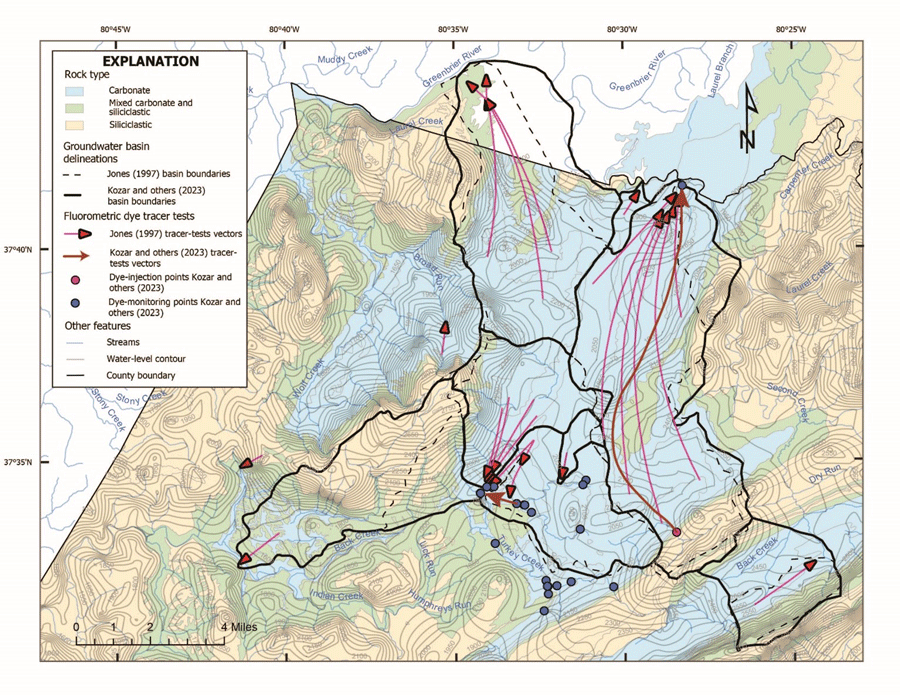
Groundwater basin boundaries delineated based on a hybrid approach, coupling traditional dye tracer tests and hydraulic gradients determined from contour lines from a potentiometric-surface map.
References Cited
Cox, C.L., and Doctor, D.H., 2021, Lidar-derived imagery and digital elevation model of Monroe County, West Virginia at 3-meter resolution: U.S. Geological Survey data release, https://doi.org/10.5066/P9TKR3XJ.
Jones, W.K., 2019, Water tracing in karst aquifers, chap. 134 of White, W.B., Culver, D.C., and Pipan, T., eds., Encyclopedia of caves (3d ed.): Elsevier, p. 1144–1155. [Also available at https://doi.org/10.1016/B978-0-12-814124-3.00134-5.]
Kozar, M.D., Doctor, D.H., Jones, W.K., Chien, N., Cox, C.E., Orndorff, R.C., Weary, D.J., Weaver, M.R., McAdoo, M.A., and Parker, M., 2023, Hydrogeology, karst, and groundwater availability of Monroe County, West Virginia: U.S. Geological Survey Scientific Investigations Report 2023–5121, 82 p., https://doi.org/10.3133/sir20235121.
Identifying Contributing Areas for a Middle Tennessee Community Drinking Water Spring With Fluorescent Dye Groundwater Tracing
Abstract
Karst aquifers are important drinking water resources in Tennessee. Groundwater in karst landscapes is susceptible to contamination due to the high level of surface and groundwater interaction. Communities create Source Water Protection Areas (SWPAs) for drinking water springs that are typically estimated, rather than delineated by a formal study. A partnership between the U.S. Geological Survey (USGS) and Tennessee Department of Conservation (TDEC) was formed to investigate karst springs, particularly those used as sources of drinking water, using fluorescent dye tracing. USGS and TDEC staff identified possible vulnerabilities that may exist within public drinking water systems based upon maturity of karst development, underlying geology, and uncertainties related to estimated recharge areas. Work began in the fall of 2022 in the community of Vanleer, located in Dickson County along the Western Highland Rim (physiographic section) of Middle Tennessee. Mississippian St. Louis and Warsaw limestones are the primary strata in this well-developed karst area. Initial dye injections provided results that highlight the need to improve the current estimated SWPA. Results from work in Vanleer continue to provide a better understanding of groundwater movement and flow path direction and give insight into surface and groundwater interactions.
Results of Tracer Testing at Pah Tempe Hot Springs, Hurricane, Utah
Abstract
Results of a dual-tracer test conducted at Pah Tempe Hot Springs near Hurricane, Utah, from mid-January 2021 to mid-April 2021, indicate that dye injected down a well discharged from the main spring (pool) and from several other springs along the Virgin River downstream from the main spring. Dye recoveries from activated charcoal placed in the springs were erratic over the course of the monitoring period and appear to have resulted in large part from highly variable adsorption of the dye onto the charcoal due to interference from bacteria and cyanobacteria that thrive in the spring water. The erratic recoveries are also likely influenced by the complex heterogeneity of the groundwater flow system in the vicinity of the Hurricane fault zone. On the basis of the relative fluorescence (intensity) observed from analysis of activated charcoal detectors, most of the dye appears to have discharged at Upper and Lower Aqueduct, Boulder, and PVC springs on the north side of the Virgin River, and Cabin springs on the south side of the river. Although dye was recovered at Pah Tempe Springs (main pool) within the first week after the injection, dye recovery from Upper and Lower Aqueduct springs occurred throughout the entire 3-month monitoring period. Dye was also recovered in all samples collected from Boulder, PVC, and Cabin springs; however, monitoring at these springs only occurred during the latter half of the study. Dye recoveries at selected springs in the downstream parts of the study area indicate that groundwater movement in the vicinity of the well is likely along preferential flow path(s) (solution-enhanced fractures and (or) faults) within the Hurricane Fault damage zone that trend sub-parallel to and likely under the Virgin River.
Continuous water samples also were collected from the main pool of Pah Tempe Springs and downstream in the Virgin River throughout the study period and analyzed for both fluorescein dye and bromide. Results of analysis of samples collected from the main spring pool appeared to be negative for dye and generally within the range of concentration for background samples collected prior to the dye injection, even during the time frame that charcoal detectors from the spring were positive for dye. Results of analysis of bromide samples from the spring also reflected natural background concentrations of bromide in the water. Results of analysis of samples collected from the Virgin River downstream from the springs and analyzed for the dye also indicated very low concentrations overall, but several periods of slightly higher values appear to coincide with activated charcoal samples collected during those same periods and considered positive. Similarly, concentrations of bromide in water samples collected from the river downstream from the springs also reflected natural background concentrations in the first part of the monitoring period. However, a notable increase in bromide concentration in the river above the natural background concentration occurred after about February 10, which may represent in part, bromide that was injected down the well. The lack of distinct breakthrough curves for both tracers at the main spring and downstream in the Virgin River appears to reflect a complex, heterogenous fracture network between the injection well and the springs that influences the movement, direction, and discharge points of tracers from the groundwater system.
Introduction
Pah Tempe Hot Springs (Dixie Hot Springs, LaVerkin Hot Springs) are located along the Virgin River near Hurricane, Utah, and issue from fractured Permian-age limestones of the Toroweap Formation. The springs discharge primarily from fractures in an alcove (main pool) along the south wall of Timpoweap Canyon (fig. 1) and from both banks of the river along a 1,500-foot reach of the channel (fig. 2) on the east side (footwall) of the northeast-trending Hurricane Fault zone (Gardner, 2018; Godwin and others, 2021). Springs also rise from multiple points in the riverbed. The springs discharge from as much as 12 feet above river stage at base flow, and total spring discharge along the reach averages about 11.5 cubic feet per second (ft3/s). Discharge from the springs has an average dissolved-solids concentration of about 9,650 milligrams per liter (Bureau of Reclamation, 1981) with a total dissolved-solids load averaging about 99,000 tons per year (Gerner and Thiros, 2014). Average water temperature of the springs is about 40 degrees Celsius.
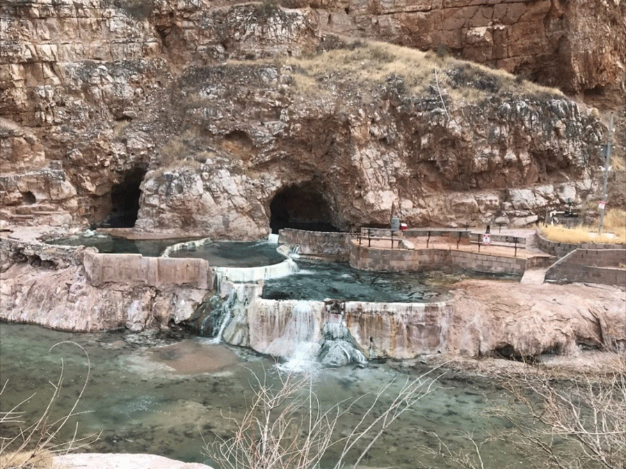
Pah Tempe main spring pool, Timpoweap Canyon, Hurricane, Utah. A former resort, Pah Tempe Springs discharge from the Toroweap Formation (Limestone) within the Hurricane Fault damage zone. Supersaturation of the spring water with respect to calcite has resulted in the deposition of large terraces as the spring water flows into the Virgin River. Greenish-white areas are bacteria and cyanobacteria. Photograph taken by Larry Spangler, U.S. Geological Survey, January 19, 2021.
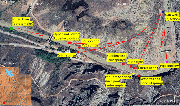
Location of spring discharge monitoring points, autosamplers, and the Bureau of Reclamation (BOR) well along the Virgin River in Timpoweap Canyon, Hurricane, Utah. Arrows represent hypothetical flow paths between the injection well and selected springs where dye was recovered during the 2021 tracer test. Dye was not recovered from any of the other springs during the 2021 tracer test.
In May–July 2020, a reconnaissance dye-tracer test was conducted to determine the discharge point of water moving through a Bureau of Reclamation well along the Virgin River upstream from Pah Tempe Hot Springs (fig. 2). On May 5, 2020, 900 grams of fluorescein (uranine) dye, a commonly used dye for groundwater tracing in karst terrains and shown to be successfully used as a tracer in geothermal systems (Adams and Davis, 1991), were injected down the well to a depth of about 190 feet, a zone of preferential flow into fractures. The dye was pre-mixed with river water in a 5-gallon bucket, then injected down the well using a peristaltic pump at a rate of about 1 liter/70 seconds. During the test, eight springs were monitored along the north and south sides of the Virgin River downstream from the injection well, as well as outflow from a group of pipes near the injection well (fig. 2). The Virgin River was also monitored downstream from all spring inflow. Total discharge from all springs during the dye test was approximately 10 ft3/s, and flow in the Virgin River was about 300 ft3/s.
Results of analysis of activated charcoal detectors collected over the 3-month period after injection showed a recovery of the dye in the main (alcove) and outflow pools of Pah Tempe Hot Springs (fig. 1). Possible or likely recoveries of the dye also were made at six other springs along the north bank. Dye was also detected in the Virgin River downstream from the springs. Straight-line distance to the main pool of the hot springs from the injection well is approximately 1,066 feet (325 meters). Maximum groundwater travel time to the main spring pool was about 9 days based on recovery of the dye from the initial detectors pulled from the spring, indicating that groundwater movement is likely along fractures and (or) conduits (solution-enhanced fractures) within the carbonate-rock aquifer from which the spring discharges.
On the basis of results obtained from the dye-tracing study in May–July 2020, a second follow-up study was initiated in January 2021. The objectives of this study were to (1) repeat the 2020 tracer test by conducting a dual qualitative and quantitative tracer test using fluorescein dye and sodium bromide, (2) determine the fractions of water in the well that discharge at the main pool of Pah Tempe Hot Springs, (3) determine a more precise time of travel between the injection well and the spring, as well as residence time of the tracers in the groundwater system, and (4) verify the discharge points at springs where dye was detected during the 2020 tracer test, and whether other springs along the Virgin River are also discharge points for the tracers.
Approach/Methods
On January 19, 2021, a dual-tracer injection was made in the Bureau of Reclamation well that was used for the May 2020 test. For this test, both sodium bromide (NaBr) and fluorescein (uranine) dye were pre-mixed with water pumped from the Virgin River into a large tank and then gravity-fed down the well through a large-diameter hose into the injection zone at approximately 190 feet from land surface. The sodium bromide was added to the tank as a salt and stirred until it was totally dissolved in the water. The dye powder was pre-mixed in a 5-gallon bucket, then poured into the tank with the bromide where they were injected as a co-mingled solution. The injection was conducted over a period of about 5 hours, but as periodic slugs. Overall, approximately 115 kilograms of sodium bromide were injected down the well in conjunction with 2 kilograms of sodium fluorescein dye.
The tracer test was partitioned into qualitative and quantitative components. For the qualitative component, activated charcoal detectors or packets were used for adsorption of the dye to determine discharge points. For the quantitative component, the fluorescein dye as well as the injected sodium bromide were analyzed in water samples that were collected on a periodic basis from ISCO automatic samplers at the main Pah Tempe Springs rise pool and downstream in the Virgin River below the input of all springflow. Water sample analyses can be used to determine a more accurate time of travel from the well to the main spring and to establish breakthrough curves for the individual tracers that can be compared.
Activated charcoal detectors were placed at most of the same springs used in the 2020 test, with several additional (previously unknown) springs also incorporated that were found later during the monitoring period. In total, 12 springs were monitored along with outflow from a set of pipes that was monitored during the 2020 test. The Virgin River was also monitored downstream from all inflow from the springs on the north and south sides of the channel, as well as springs rising in the bed of the channel that could not be individually monitored. Three days prior to the injection on January 19, charcoal detectors were placed in all springs and in the Virgin River for the purpose of determining the relative intensity of background fluorescence from natural organic materials in the water that can potentially mask detection of the injected dye (Alexander, 2005). This set of background detectors was pulled and replaced with another set of detectors in the morning of the day of the injection. Sites monitored with charcoal detectors were assigned unique names for this study, and from upstream to downstream along the Virgin River (fig. 2) were as follows:
-
Pipe outflow (group of PVC pipes discharging spring water into the river) – north side
-
Waterfall spring – south side
-
Conduit spring – south side
-
Pah Tempe Spring (main pool) – south side
-
Terrace spring – north side
-
Pole spring – north side
-
Bubbling spring – north side
-
Cairn springs – north side
-
PVC spring – north side
-
Boulder spring – north side
-
Cabin springs – south side
-
Aqueduct spring (upper) – north side
-
Aqueduct spring (lower) – north side
-
Virgin River below springs
The dye was recovered on 6–12 mesh activated charcoal that was placed into fiberglass screen packets suspended from concrete weights or attached to tent stakes placed in or just downstream from the spring discharge points. In most cases, duplicate packets were employed to serve as back-ups if one of the packets was damaged or lost and also as a verification of the result from its companion packet. The dye packets were left in situ for a period that correlated with the exchange of bottle trays in the autosamplers (refer to section on quantitative component of study) every 3 days initially, extending to longer intervals as the monitoring period progressed. At the end of each time interval, the detectors were exchanged with new ones.
The detectors were transported back to the Utah Water Science Center (UTWSC) laboratory in Salt Lake City where the dye was extracted from the activated charcoal with a 5-percent solution of 70-percent isopropyl alcohol and potassium hydroxide, a commonly used eluent for elution of dyes (particularly fluorescein) from charcoal (Quinlan, 1989). Presence of the dye in some samples was determined by visual observation if the concentration was high enough. Most samples, however, were analyzed on a Shimadzu RF-5301PC scanning spectrofluorometer. Results of analysis were reported qualitatively in terms of negative (no dye was detected), positive (dye was observed instrumentally), very positive (dye was observed visually in the solution) or potentially positive (dye response meets certain criteria but not able to be corroborated). Evaluation of the results of analysis of the scanned samples for the presence of dye is largely based on the protocols used by Crawford Hydrology Laboratory (2019) at Western Kentucky University.
In addition to the use of activated charcoal for the adsorption of dye during the study, two ISCO 3700 series automatic water samplers were employed to collect water samples for both the dye and sodium bromide on a timed basis. These samplers were installed at the Pah Tempe Springs main pool and downstream in the Virgin River at the same location as the charcoal detectors (fig. 2). The autosamplers were programmed to collect 400-milliliter (mL) samples on a 2-hour basis at the start of the test, but this interval was increased later in the monitoring period to 4, 6, and 8 hours until the end of the study. In addition, the autosamplers were set up on an offset schedule to enhance the sampling coverage throughout the monitoring period. Three days prior to the dye injection, samples were also collected on a 2-hr basis to determine the amount of natural fluorescence in the water that could potentially interfere with the detection and analysis of the fluorescence attributed to the dye. Unlike the charcoal detectors which can only be used to establish hydraulic connections from input to output, the purpose of the autosamplers was to obtain a record of the travel time of the dye and the bromide as the tracers moved from the well to the main spring and downstream in the river below the other spring inputs. This would result in breakthrough curves for each of the tracers that could be compared and from which other data could be extracted such as first arrival of the tracer at the sampler, time to peak arrival and concentration, and residence time of the dye and bromide in the groundwater system. Although the adsorption of dye onto activated charcoal is a passive, cumulative process, water samples represent the instantaneous (real-time) concentration of dye in the water.
At the end of each sampling period after 24 samples had been collected, the bottle trays were replaced with a new cleaned bottle tray, and the sampler was re-programmed for the next sampling cycle. The bottles were subsequently moved to an onsite cabin where the samples were split into 250-mL and 125-mL polyethylene bottle subsamples for analysis of the fluorescein dye and bromide, respectively. Samples for dye analysis were transported to the UTWSC laboratory in Salt Lake City where they were analyzed on a Turner Designs TD700 series filter fluorometer. Samples for bromide analysis were transported to the University of Utah Department of Geology and Geophysics laboratory where they were analyzed by ion chromatography.
Results of Analysis and Discussion
Activated charcoal has a strong affinity for the sorption of dyes; however, that sorption can be highly variable, sometimes producing substantially different or inconsistent values that can be challenging to evaluate with respect to whether the sample is positive for dye. These factors include the length of time the charcoal is in the water, velocity of the water, and the location of the charcoal in the spring or stream. Dye recoveries at the monitored sites varied between detectors placed near each other at the same location, and over the period of monitoring, which increased over time. Velocities also ranged from slow (pools) to greater than 1 foot/second. As a result, dye recoveries could not be verified at some sites or at selected times. In most cases dual detectors were placed at each of the monitoring sites, and thus, would be expected to yield similar results with respect to adsorption of the dye. The variability in dye recovery observed throughout the monitoring period, however, is interpreted to be primarily the result of a heavy coating of white, non-photosynthetic filamentous bacteria and cyanobacteria (fig. 1) (Hannah Bonner, Utah Division of Water Quality, written commun., June 12, 2024) on the packet itself, which impeded the sorption of dye onto the charcoal within the packet. The bacterial coating appears to have occurred very rapidly (within hours) of placement of the detectors in the springflows, resulting in a substantially reduced window for adsorption of the dye. Coatings on detectors that were only 1 foot apart (opposite ends of the weighted assembly used to suspend the detectors) also were observed to be variable in some instances, resulting in a substantial difference in values of fluorescence and thus dye adsorption between the two detectors. In addition, positive dye recoveries were obtained intermittently at some sites, which again, may have resulted from variable adsorption resulting from bacterial coatings, or possibly other factors influencing movement of the dye through the fractured network from the well to the springs.
Results of Activated Charcoal Analysis
During the 2021 tracer test, fluorescein dye was recovered from one or more charcoal samples at the following springs: Upper and Lower Aqueduct springs, Pah Tempe main spring (pool), Boulder and PVC springs, and Cabin springs (fig. 2). Samples collected from Pah Tempe main spring on January 22 and 25, within 1 week of the injection, were positive, and samples collected on January 29, February 16, and March 2 were also potentially positive. All other samples collected from the main spring appeared to be negative. On several occasions, detection of dye at the Pipe outflow, closest monitoring site to the well, was interrupted by human tampering, making an evaluation of results from this site problematic. Nonetheless, potentially positive results were observed on several occasions. Dye was not detected at any of the other sites monitored during the 2021 tracer test. Dye was also recovered from numerous samples collected from the Virgin River downstream from all the springs. During the 2020 tracer test, dye was also recovered at Pah Tempe main spring and in the Virgin River downstream from the springs. Dye also appeared to have been recovered at Upper Aqueduct and Bubbling springs, and at Sand spring, which was not monitored during the 2021 test due to low-flow conditions. In addition, dye was potentially recovered at Lower Aqueduct, Pole, and Terrace springs (fig. 2). Boulder and PVC springs (north side of river) and Cabin springs (south side of river) were not monitored during the 2020 test, in part because they were inundated by the Virgin River and therefore, not visually apparent.
Overall, the most positive (greatest fluorescence) samples during the 2021 dye test were from sites farthest downstream from the injection well, including Upper and Lower Aqueduct, and Boulder and PVC springs on the north side of the Virgin River, and Cabin springs on the south side of the river, directly across from Boulder spring (fig. 2). Straight-line distance from the well to Lower Aqueduct spring, the farthest point downstream where dye was detected, is about 1,400 feet (425 meters). Earliest detection of dye at Upper Aqueduct spring was on January 22, about 3 days after injection, and dye was still detected in the spring on March 18, 2 months after injection. Samples were very positive on January 25 and February 2, but negative on January 29, indicating as previously noted, bacterial interference in adsorption of the dye, or heterogeneity within the fracture network in the fault zone, including the possibility that dye could be transported along multiple flow paths (for example, fractures and solution-enhanced fractures) between the well and the spring. Earliest detection of dye at Lower Aqueduct spring was on January 25, about 6 days after injection and continued to be detected in many samples until March 18, when monitoring was concluded. Boulder, PVC, and Cabin springs were not identified prior to the January 19, 2021 dye injection, and monitoring at these springs did not begin until mid-February. Dye was detected at these springs based on samples collected on March 2 (PVC spring) and March 18 (Boulder and Cabin springs). It is very likely that dye was present in water from these springs prior to when monitoring began based on the proximity to and results of analysis of samples from the Aqueduct springs. Monitoring at all three locations continued until April 16 when monitoring was discontinued. Very positive samples (visually observed in elutant) from this period indicate that dye was still present in the groundwater system 3 months after the injection.
Analysis of charcoal samples from Pah Tempe main spring on the south side of the river and from several sites on the north side of the river across and upstream from the main spring showed that fewer samples were positive for dye and that relative fluorescence of those samples was considerably lower in comparison to samples collected from springs downstream along the river. This unexpected difference in detection of the dye between upstream sites closer to the injection well and downstream sites indicates a complex system of fractures with varying connectivity and implies that the greatest mass of dye injected down the well and thus groundwater moving through the well, is transported along preferential flow paths (solution-enhanced fractures and possibly faults) that lie sub-parallel to (north of), and likely under the Virgin River. Although Pah Tempe main spring is the largest single discharge point in the study area, results from both dye tests indicate that movement of groundwater to the spring may be along a secondary zone of fractures that are poorly connected to the principal flow path(s) that conduct water to springs downstream from the main spring. Godwin and others (2021) also recognized the strong heterogeneity in fracture flow within the Hurricane Fault damage zone at Pah Tempe Hot Springs. The complexity of the groundwater flow system is not only shown by the erratic results obtained from samples at Pah Tempe main spring over the monitoring period but also by the apparent lack of any positive results at Waterfall and Conduit springs only 100 feet upstream from the main spring (fig. 2).
Dye was also monitored downstream in the Virgin River below all springflow inputs along both sides of the river as well as from flow discharging into the river from the streambed. The first detection of dye in the river downstream was on January 25, about 6 days after injection. Dye was then detected in the river in most samples subsequently collected, with the last detection occurring in a sample collected on March 18, 2 months after injection. Although results of dye analyses (fluorescence) tended to be erratic, overall recoveries from the river samples generally coincided with positive recoveries observed upstream at springs during the same time period, as would be expected. Nonetheless, variations in dye recovery that were observed on detectors collected from the same time period, are interpreted to be due to location of the detectors in the river and to a lesser degree, the effects of bacterial coatings on the detectors, which is substantially less in the river. An assumption was made that flow in the channel and thus dye concentration, was fairly uniform (well-mixed) across the channel. Because the detectors were located near the right bank (looking upstream) and adjacent to the autosampler, rather than in the middle of the channel, however, it may have been possible in some cases that stream currents had an effect on the transport of dye down the channel, particularly as changes in discharge occurred, resulting in the variability in adsorption (fluorescence) observed.
Results of Water Sample Analysis
Results of analysis of water samples collected from the Pah Tempe main spring pool were characterized by dye values that ranged from only 0.01 to 0.06 parts per billion (ppb). Because this range in values was also within the range in values for natural background fluorescence in the spring water prior to the dye injection, no samples could be considered unequivocally positive for dye, even during the first week after injection when charcoal samples were positive. This phenomenon may be explained in part, by the very low concentrations of dye in the water that were not detectable in an instantaneous sample taken every 6 hours, compared to the cumulative adsorption of the low-level concentrations of the dye on activated charcoal over a multi-day period. Results of analysis of water samples collected from the Virgin River downstream from the spring inputs were characterized by values that ranged from 0.03 to 0.13 ppb. Values of background fluorescence in the river water prior to dye injection also overlapped values of samples collected after the injection, generally falling between 0.04 and 0.08 ppb. Nonetheless, values of samples with slightly higher fluorescence (greater than or equal to about 0.12 ppb) appear to coincide with activated charcoal samples collected during the same periods (January 27–29, January 31–February 2, and possibly after March 11) that were positive. Positive recoveries from charcoal collected at Pah Tempe main spring on January 25 are also likely reflected in samples collected at the Virgin River sampler on January 24. Overall, results of analyses of water samples collected from Pah Tempe main spring and to a lesser degree from the Virgin River downstream from the springs, cannot be represented as distinct breakthrough curves, but rather as erratic responses to the dye as it discharged from the groundwater system.
Results of analysis of bromide at Pah Tempe main spring and in the Virgin River yielded similar results. Bromide concentrations in the main spring pool remained essentially at background levels throughout the monitoring period, ranging between 3.1 and 3.3 parts per million (ppm), which represents the natural concentration of bromide in the water discharging from the main spring (fig. 3). Bromide concentrations in the Virgin River below the inflow of all springs also were typically at background levels (1.5 to 1.75 ppm) for the first part of the monitoring period until about February 3, after which concentrations decreased abruptly to less than 1 ppm. Concentrations subsequently rose to levels slightly above previously measured background levels (2.0 ppm), after which concentrations again increased slightly to between 2.2 and 2.3 ppm, then stayed constant for the remainder of the monitoring period (fig. 3).
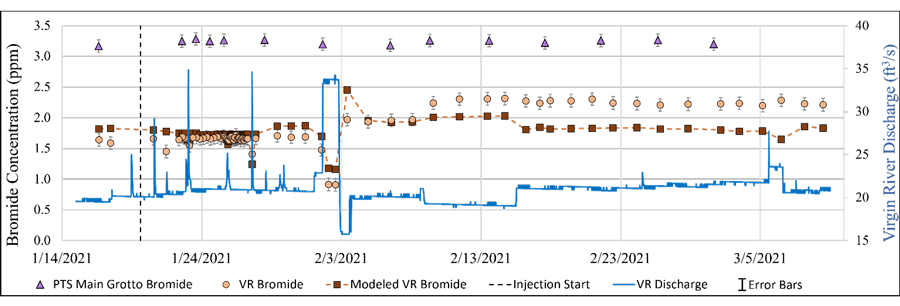
Graph showing bromide concentration at Pah Tempe main spring pool, and relations between bromide concentration in the Virgin River downstream from spring inputs, discharge of the Virgin River, and modeled bromide concentration based on Virgin River discharge. PTS, Pah Tempe Spring; VR, Virgin River; ppm, parts per million; ft3/s, cubic feet per second. Bromide data are preliminary or provisional and are subject to revision. They are being provided to meet the need for timely best science. The data have not received final approval by the U.S. Geological Survey (USGS) and are provided on the condition that neither the USGS nor the U.S. Government shall be held liable for any damages resulting from the authorized or unauthorized use of the data.
Relations Between Discharge and Bromide Concentration
Discharge of the Virgin River is monitored at U.S. Geological Survey streamflow-gaging station Virgin River AB LA Verkin Creek NR LA Verkin, UT - 09406100 (U.S. Geological Survey, 2021) about 1.5 miles downstream from Pah Tempe Springs and reflects flow in the river as well as flow from all of the springs; no significant inflows occur between the spring inflows and the gage. During the monitoring period, river discharge generally ranged between 20 and 22 ft3/s, with intermittent spikes in flow to as much as 35 ft3/s that reflect upstream (1 mile above Pah Tempe Springs) fluctuations in the amount of water being diverted from the river. This abrupt increase/decrease in flow was particularly noteworthy on February 2–3, with a decrease in the bromide concentration as river discharge increased, followed by an increase in the bromide concentration as river discharge decreased (fig. 3). Afterwards, bromide concentration in the river increased slightly and remained constant (2.2 to 2.3 ppm) for the remainder of the monitoring period, and discharge also remained fairly constant, varying within a 3-cubic foot/second range for the remainder of the study.
Virgin River discharge was used in a two end-member mixing model to differentiate between bromide concentration that is natural in the river and that originating from the sodium bromide injected down the well. These relations showed that modeled bromide concentrations in the river before about February 7 were very similar to measured concentrations, whereas modeled bromide concentrations after about February 10 were significantly less than measured concentrations (typically about 0.45 ppm) (fig. 3). This indicates that measured concentrations of bromide in the Virgin River after about February 10 (2.2 to 2.3 ppm) may be in part, from the injected bromide in addition to the natural concentration of bromide (1.5 to 1.75 ppm) in the river water. The relatively constant low-level bromide concentrations measured during this period also support the hypothesis of a complex, heterogenous fracture network within the Hurricane Fault damage zone that conducts groundwater along multiple flow paths to springs discharging along the Virgin River.
References Cited
Adams, M.C., and Davis, J., 1991, Kinetics of fluorescein decay and its application as a geothermal tracer: Geothermics, v. 20, issues 1–2, p. 53–66. [Also available online at https://doi.org/10.1016/0375-6505(91)90005-G.]
Alexander, S.C., 2005, Spectral deconvolution and quantification of natural organic material and fluorescent tracer dyes, in Sinkholes and the Engineering and Environmental Impacts of Karst, Proceedings of the 10th Multidisciplinary Conference, September 24–28, 2005, San Antonio, Texas: American Society of Civil Engineers, Geotechnical Special Publication No. 144, p. 441–448.
Gardner, P.M., 2018, Effects of groundwater withdrawals from the Hurricane Fault zone on discharge of saline water from Pah Tempe Springs, Washington County, Utah: U.S. Geological Survey Scientific Investigations Report 2018–5040, 41 p., https://pubs.usgs.gov/publication/sir20185040.
Gerner, S.J., and Thiros, S.A., eds., 2014, Hydrosalinity studies of the Virgin River, Dixie Hot Springs, and Littlefield Springs, Utah, Arizona, and Nevada: U.S. Geological Survey Scientific Investigations Report 2014–5093, 47 p., http://dx.doi.org/10.3133/sir20145093.
Godwin, S.B., Nelson, S.T., McBride, J.H., Rey, K.A., Tingey, D.G., Tingey, E., and Carling, G., 2021, Thermal spring system plumbing across a major normal fault—Pah Tempe, Utah, USA: Lithosphere, v. 2021, article ID 3364591, 17 p., https://doi.org/10.2113/2021/3364591.
U.S. Geological Survey, 2021, USGS water data for the Nation: U.S. Geological Survey National Water Information System database, accessed June 2021, at https://doi.org/10.5066/F7P55KJN.
Disclaimers
Any use of trade, firm, or product names is for descriptive purposes only and does not imply endorsement by the U.S. Government.
Although this information product, for the most part, is in the public domain, it also may contain copyrighted materials as noted in the text. Permission to reproduce copyrighted items must be secured from the copyright owner.
Suggested Citation
Kuniansky, E.L., and Spangler, L.E., eds., 2024, U.S. Geological Survey Karst Interest Group proceedings, Nashville, Tennessee, October 22-24, 2024: U.S. Geological Survey Open-File Report 2024-1067, 109 p., https://doi.org/10.3133/ofr20241067.
ISSN: 2331-1258 (online)
| Publication type | Report |
|---|---|
| Publication Subtype | USGS Numbered Series |
| Title | U.S. Geological Survey Karst Interest Group proceedings, Nashville, Tennessee, October 22-24, 2024 |
| Series title | Open-File Report |
| Series number | 2024-1067 |
| DOI | 10.3133/ofr20241067 |
| Publication Date | November 01, 2024 |
| Year Published | 2024 |
| Language | English |
| Publisher | U.S. Geological Survey |
| Publisher location | Reston, VA |
| Contributing office(s) | Office of the Associate Director for Water |
| Description | iv, 109 p. |
| Online Only (Y/N) | Y |
| Additional Online Files (Y/N) | N |