Calibration of the Stream Salmonid Simulator (S3) model to estimate annual survival, movement, and food consumption by juvenile Chinook salmon (Oncorhynchus tshawytscha) in the restoration reach of the Trinity River, California, 2006–18

John M. Plumb; Russell W. Perry; Kyle De Juilio

doi:10.3133/ofr20241070

Calibration of the Stream Salmonid Simulator (S3) Model to Estimate Annual Survival, Movement, and Food Consumption by Juvenile Chinook Salmon (Oncorhynchus tshawytscha) in the Restoration Reach of the Trinity River, California, 2006–18

Open-File Report 2024-1070

Prepared in cooperation with U.S. Bureau of Reclamation

By: John M. Plumb, Russell W. Perry, and Kyle De Juilio

https://doi.org/10.3133/ofr20241070

Metrics

Web analytics dashboard Metrics definitions

Links

Document: Report (7.9 MB pdf) , HTML , XML
Download citation as: RIS | Dublin Core

Acknowledgments

We are grateful to the many entities, agencies, and field staff that have collected and provided data to inform the Stream Salmonid Simulator (S3) as applied to the Trinity River. From our colleagues at the U.S. Geological Survey (USGS), we extend gratitude to Ty Hatton for his diligence and help in data processing. From outside the USGS, we extend thanks to staff at the U.S. Fish and Wildlife Arcata, California for providing the weekly abundances of juvenile fall Chinook salmon (Oncorhynchus tshawytscha) passing the fish trap, allowing us to fit the S3 model and estimate its primary parameters, and for providing the spawning escapement estimates, which are foundational and integral to all S3 simulations.

Executive Summary

The Trinity River is managed in two sections: (1) from the upper 64-kilometer “restoration reach” downstream from Lewiston Dam to the confluence with the North Fork Trinity River, and (2) the 120-kilometer lower Trinity River downstream from the restoration reach. The Stream Salmonid Simulator (S3) has been previously applied to these reaches and the Klamath River. To estimate fish growth, past S3 calibration efforts in the Trinity and Klamath Rivers used maximum likelihood methods that considered only the abundance of juvenile Chinook salmon (Oncorhynchus tshawytscha) passing a fish trap to estimate survival and movement parameters, but not fish consumption. Previous calibrations did not estimate the average proportion of maximum consumption (C_y) when estimating survival (S_y) and movement (M₀_y) parameters across years (y) of data, but because no other information was available in the literature a fixed value of C_y=0.66 was assumed. Therefore, the goal of this report is to present an alternative approach that calibrates the S3 model to multivariate data (that is, abundance and size), enabling the estimation of the average proportion of maximum consumption, in conjunction with survival and movement parameters for a particular migration year. We fit the S3 model to individual years of weekly trap abundance estimates and mean fish sizes (fork length) at the Pear Tree Gulch (hereafter referred to as Pear Tree) fish trap representing the restoration reach. We used the Earth Mover’s Distance (EMD) as the objective value to be minimized in parameter optimization. This approach estimated survival, movement, and consumption parameters for each migration year. Because we had information on the abundance of natural and hatchery produced juvenile salmon at the fish traps, we estimated survival and movement for natural and hatchery fish.

S3 is a deterministic life-stage-structured population model that tracks daily growth, movement, and survival of juvenile Chinook Salmon. A key theme of the model is that river discharge affects habitat availability and capacity, which in turn drives density-dependent population dynamics. To explicitly link population dynamics to habitat quality and quantity, the river environment is constructed as a one-dimensional series of linked habitat units, each of which has an associated daily timeseries of discharge, water temperature, and useable habitat area or carrying capacity. In turn, the physical characteristics of each habitat unit and the number of fish occupying each unit drive survival and growth within each habitat unit and movement of fish among habitat units.

The physical template of the restoration reach of the Trinity River was classified into 356 meso-habitat units comprised of runs, riffles, and pools. For each habitat unit, we developed a timeseries of daily discharge, water temperature, amount of available spawning habitat, and fry and parr carrying capacity. Capacity time series were constructed using state-of-the-art models of spatially explicit hydrodynamics and quantitative fish habitat relationships developed for the Trinity River. These variables were then used to drive population dynamics such as egg maturation and survival, and in turn, juvenile movement, growth, and survival.

We estimated movement, survival, and consumption parameters by calibrating the model to 12 years of weekly juvenile abundance estimates and fish sizes at the Pear Tree fish trap near the downstream end of the restoration reach. We estimated parameters for 12 years that included a wide range of female spawner abundances (1,414–11,494) and water year types (critically dry–extremely wet). We contrast the estimated parameters to the corresponding number of female spawners and the total annual volume of water discharged for the Trinity River (Trinity River Restoration Program; https://www.trrp.net/restoration/flows/summary/).

The calibration consisted of replicating historical conditions as closely as possible (for example, discharge; temperature; spawner abundance, spawning location and timing, and hatchery releases), and then running the model to predict weekly abundance passing the trap location from each brood year of adults and subsequent migration year of their juvenile progeny. Because density-dependent movement was favored in past evaluations, we estimated S3 parameters based on density-independent survival and density-dependent movement. Likewise, each year’s estimated survival parameter for natural (S_N_y) and hatchery (S_H_y) fish may be interpreted as the mean daily survival probability from emergence or hatchery release to the Pear Tree fish trap. Under density dependence, the estimated movement parameter for natural (M_0N_y) and hatchery (M_0H_y) fish represents the intercept of the Beverton-Holt model; the probability of remaining in a habitat at near-zero abundance.

We estimated C_y by using EMD and incorporating abundance and fish size into model calibration. Average daily proportions of maximum consumption, $\bar{C}$ , across the years were generally high ( $\bar{C}$ =0.640; standard deviation (SD) SD=0.176), suggesting that fish were feeding at about two-thirds of expected maximum consumption rates. This average proportion of maximum consumption, $\bar{C}$ is very similar to what has been assumed ( $\bar{C}$ =0.66) in previous Trinity and Klamath River S3 calibration and simulation efforts. In 2017, we estimated the lowest C_y, suggesting lower average consumption for juvenile salmon in high-discharge water years. When this high discharge year was excluded, there was no apparent trend in C_y with annual water volume. Estimates of survival showed little trend over the range in spawner abundances, but a trend towards higher natural and hatchery fish survival with higher annual volumes of water was apparent. Over the 12 years, the average survival of hatchery fish was ${\bar{S}}_{H}$ =0.888 (SD=0.079) and the average survival natural fish was ${\bar{S}}_{N}$ =0.969 (SD=0.01).

With respect to fish movement, we estimated higher M_0N_y and M_0H_y with higher annual volumes of water in the Trinity River. Higher M_N0_y or M_H0_y suggest greater probability of remaining in a habitat at low fish densities, with potential for density-dependent processes in movement to occur. The highest M_0N_{y =} 0.676 was estimated during brood year 2012, and the overall average for natural fish was ${\bar{M}}_{0 N}$ =0.276 (SD=0.188) and for hatchery fish was ${\bar{M}}_{0H}$ =0.467 (SD=0.235). Under the Beverton-Holt model, as M_0N_y or M_0H_y approach zero, there is less capacity for change in fish movement as fish density increases.

The S3 model was initialized with only the spatiotemporal distribution of spawners, so it performed well at capturing the essential outmigration features that are ultimately governed by rates of growth, movement, and mortality. We used a new optimization method that could accommodate multivariate data on abundance and fish size collected at the Pear Tree fish trap, enabling the calibration of S3 to estimate five parameters for 12 separate years of data. Incorporating weekly fish size data for each year in our parameter optimization process made the estimation of C_y possible and represents a step forward in the fitting of the S3 model to fish trap data for the purposes of parameter calibration and the estimation of growth parameters with respect to annual conditions. We identified lack of fit and adding important effects into the S3 model may improve the S3 estimation and simulation of water scenarios.

The Trinity River Restoration Program (TRRP) Science Advisory Board recommended that the TRRP focus on developing core elements of a decision support system (DSS; Buffington and others, 2014). Toward that end, the habitat and S3 models described in this report are both core elements of the DSS. The structure of S3 makes it a particularly useful fish production model for the DSS because population dynamics are sensitive to (1) water temperature, (2) daily discharge management, and (3) habitat quality and quantity. Each of these variables are key management parameters under consideration in the TRRP. As such, the S3 model may provide valuable insights into the potentially variable effects of different management decisions on the Trinity River.

Introduction

The underlying restoration strategy of the Trinity River Restoration Program (TRRP) is in restoring the physical processes (given constraints of the existing infrastructure) and managing discharges to meet micro-habitat and thermal needs of anadromous salmonids. Restoring habitat and discharges should provide spawning and rearing opportunities for juvenile salmon. The TRRP is implemented under an Adaptive Environmental Assessment and Management (AEAM) framework (U.S. Department of the Interior, 2000). Implementation of the AEAM process is outlined in the TRRP Integrated Assessment Plan. The Integrated Assessment Plan identifies key assessments necessary to provide short-term and long-term feedback on the effectiveness of the TRRP in meeting specific management objectives as well as long-term programmatic goals.

For evaluating management objectives to be implemented by the TRRP, a subcommittee of the TRRP Fish Workgroup was established to initiate the development of a Trinity River fish production model (Trinity River Restoration Program and ESSA Technologies, Ltd., 2009). Recommendations by the TRRP Science Advisory Board further motivated the development of a Trinity River fish production model as part of the TRRP decision support system. The fish production model should enable the TRRP to evaluate:

1. Response of fish production to different discharge management alternatives, including variable discharge levels during specific life stages;
2. Response of fish production to different channel rehabilitation actions;
3. Overall restoration strategy of the TRRP using potential habitat estimates to attain fish population goals;
4. Temperature response of fish growth and resulting production; and
5. Growth/size of fish in response to different discharge/temperature alternatives and relate this to potential survival.

Given the required outputs of a fish production model for the TRRP, the Stream Salmonid Simulator (S3) was selected as the modeling framework for the Trinity River decision support system. S3 is a population model that simulates daily growth, movement, and mortality of freshwater life stages of riverine salmonids. The model is spatially explicit, representing the river as a linked series of meso-habitat units, each with associated discharge, water temperature, and habitat characteristics that are linked to demographic processes to drive population dynamics using the following modeling framework:

1. A rigorous mathematical basis for spatially explicit population dynamics in a riverine environment;
2. Movement models that reflect recent advances in modeling juvenile salmon migration;
3. Mechanistic growth models parameterized for anadromous salmonids of interest; and
4. Implementation of the model in an open-source modeling platform.

We began development of S3 for the Klamath River in 2012, following completion of River Basin Model-10 for the Klamath (Perry and others, 2011) and Trinity Rivers (Jones and others, 2016). River Basin Model-10 is a spatially explicit water-temperature model, which provided simulations of daily water temperatures and discharge that are required as input for the S3 model. Since 2012, our modeling team has (1) developed new growth models for juvenile Chinook salmon (Oncorhynchus tshawytscha; Perry and others, 2015; Plumb and Moffitt, 2015) and Coho salmon (O. kisutch; Manhard and others, 2018), (2) developed new analytical methods for quantifying habitat suitability criteria needed for modeling available fish habitat (Som and others, 2018a), and (3) constructed the underlying S3 modeling framework that is implemented in the R statistical programming language (R Core Team, 2022; Perry and others, 2018a). The application, parameterization, and calibration of S3 to the Klamath River and the restoration reach of the Trinity River is publicly available (Perry and others, 2018b; Plumb and others, 2023).

This report describes the calibration of the S3 model parameters with the primary goal of estimating annual values of food consumption. Because of the generally cold-water temperatures and the potential for food limitations for juvenile salmon in the Trinity River, resource managers have questions about the consumption and growth of rearing and migrating juvenile salmon. The S3 model incorporates a module of the “Wisconsin” bioenergetics model for juvenile salmon (Stewart and Ibarra, 1991), which has been used since the 1980s to estimate fish consumption from empirical measurements of fish size over time. The bioenergetics model estimates consumption as proportion of the fish’s maximum possible consumption ( $\bar{C}$ ), which is expressed as a function of body size and temperature. Past S3 calibrations and simulations had to assume a fixed proportion of maximum consumption over the growth period with $\bar{C}$ =0.66 because of the potential of confounding with survival and movement parameters. Estimating food consumption by juvenile salmon for the S3 model is important because (1) growth directly affects S3 estimation of biomass produced and (2) the TRRP has identified a need to better incorporate food consumption and growth in S3 model simulations. In response to this need, we calibrate the survival, movement, and consumption parameters for S3 to individual years of weekly trap abundance estimates and mean fish sizes (fork length, [FL]). By incorporating the mean fish size into model calibration, the confounding between survival, movement, and consumption parameters could be alleviated. After model calibration, we simulate juvenile Chinook salmon as they migrate from natal spawning grounds to the Pear Tree fish trap, for each year and week, and compare this output to the estimates of abundance and mean size of fish passing the Pear Tree fish trap. This report extends upon previous calibration efforts reported by Perry and others (2018c) and Plumb and others (2023). We detail model construction, parameterization, and calibration, and we evaluate how well the production of juvenile Chinook salmon predicted by S3 compares to observed data collected at the Pear Tree fish trap. This report is a companion to Perry and others (2018a), which details the general model structure and sub-models that are common across applications of S3 to Chinook salmon in the Klamath and Trinity Rivers (Perry and others 2018b, c).

Study Site

In this report, we focus on the 64-kilometer section known as the restoration reach of the Trinity River (Perry and others, 2018c). This section of the Trinity River is critical habitat used by several anadromous salmonids, including spring and fall-run Chinook salmon, Coho salmon, and Steelhead trout (Oncorhynchus mykiss), representing an important fishery to native Tribes, residents, and tourists. The characteristics of the river vary and are described in detail by Perry and others (2018b).

Since 2000, the TRRP has worked to improve and restore fish habitat and to promote fluvial geomorphic processes in the restoration reach of the river, which spans from Lewiston Dam downstream to the confluence with the North Fork Trinity River. Fish populations in the restoration reach are monitored intensively; spawner surveys are performed annually to estimate spawner abundance. Juvenile production in the restoration reach is monitored using mark-recapture methods and rotary screw traps fished near Pear Tree Gulch, about 1 kilometer upstream from the North Fork Trinity River confluence. The data collected from the fish traps (Pinnix and others, 2022) are integral to this report because fish catch at the trap provides estimates of fish abundance and fish size used to calibrate the S3 model parameters.

Methods

The relevant key features of the S3 model are (1) the optimization of parameters from multivariate data on fish abundance and size and (2) annual estimates of S3 survival, movement, and consumption parameter values for juvenile salmon with respect to key environmental variables (such as the number of spawners, water year type, and the total annual natural volume of water for the Trinity River). Perry and others (2018a) detail the mathematical structure of the S3 model, and Plumb and others (2019) provide an example (in the Klamath River) of using S3 simulations to assess the effects of discharge and temperature management.

S3. Habitat Template and Physical Inputs

The spatial domain of the S3 model is defined by a one-dimensional representation of discrete meso-habitat units (MHU). MHUs are spatially referenced by their upstream and downstream boundaries and measured as the distance in river kilometers from the Klamath River confluence. The length of a MHU is the difference between its upstream and downstream boundaries.

To define the MHU boundaries for the Trinity River, field biologists familiar with the river delineated MHUs at transitions between three distinct meso-habitat types: riffles, runs, and pools. The restoration reach was partitioned into 356 contiguous MHUs and classified by meso-habitat type (Perry and others, 2018c). MHU delineations were drawn perpendicular to the river discharge using orthographic satellite imagery (ESRI, 2011). Disagreements were few and arbitrated via discussion, and ultimately MHU boundaries were decided with full consensus among group members.

To define the quality and quantity of fish habitat within each MHU we used output from a two-dimensional hydraulic model (Bradley, 2016) and micro-habitat models (Som and others, 2018b). We represented each MHU as a polygon (Perry and others, 2018c), which allowed us to assign cells of the finer-scale hydraulic model to each MHU. Output from micro-habitat models were then applied to the cells of the two-dimensional hydraulic model and summarized over each MHU to construct the one-dimensional inputs required by the S3 model (Perry and others 2018c).

Biological Inputs

The S3 model relies on the two primary forms of biological inputs to simulate population dynamics: (1) female spawners and (2) juvenile fish entering from tributaries and hatchery releases.

Female Spawners

To develop inputs for the number of female spawners, spawner survey data (Chamberlain and others, 2012; Rupert and others, 2017a, b; Gough and others, 2019, 2021) were summarized as a weekly time-series of redd counts by survey reach. Of 14 spawning survey reaches between Lewiston Dam and the Klamath River confluence, 7 reaches fall within the restoration reach (Perry and others, 2018c, Plumb and others, 2023). Model simulations tracked two subpopulations of early (spring) and late (fall) spawning Chinook salmon in the same manner as Perry and others (2018c). To construct model inputs, we mapped the reach-level redd survey data to each MHU and converted the weekly redd counts to daily redd counts by dividing weekly counts by seven. Within each survey reach, daily redds were then distributed to MHUs proportional to the distribution of daily redd capacity in each survey reach.

Juveniles from Hatchery Production

We included hatchery releases of age-0 (fingerling) juvenile Spring and Fall Chinook salmon as separate sub-populations in S3. Data on hatchery releases of Chinook salmon were obtained from the Regional Mark Information System database (https://www.rmpc.org/). Juvenile Chinook salmon from the Trinity River hatchery were released in batch releases that were predominantly volitional. Volitional releases were initiated by opening a gate on a hatchery pen so fish could freely enter the Trinity River. On average, 12 days lapsed (range: 8–17 days) before the last fish exited the pen. As a result, each release had a start and end date. We approximated the daily number of fish released by partitioning the batch size evenly across the days of the volitional release. Typically, more than one batch was released at a time. For input to S3, the total number of hatchery fish entering the river each day was the sum of the daily approximated number of fish released from all concurrent batches. The Trinity River hatchery also releases cohorts of several other salmonid species throughout the year, but interactions of these salmonids with Chinook salmon are not currently (2024) modeled in S3.

In addition to daily hatchery release numbers, S3 required the mean weight of hatchery fish entering the river. Prior to release, each batch was sampled to estimate the mean weight of individual fish. To calculate the mean weight of fish entering the river in S3, we used the mean weight of fish in concurrent batch releases, weighted by the batch-specific daily release numbers. Daily release numbers and weighted-mean fish weights were computed separately for Spring and Fall Chinook salmon input data. Simulated hatchery inputs entered the river just below the dam, and the two sub-populations were tracked separately in S3. The mean weight of fish was converted to fork-length (FL; Perry and others, 2018b) to classify the life stage of hatchery inputs as fry, parr, or smolt, upon river entry.

Juveniles from Tributaries

One of the four major tributaries to the Trinity River, Canyon Creek, is thought to contribute to the production of juvenile salmon above the Pear Tree fish trap. Because information on the production of juveniles from tributaries in the Trinity River is limited, we used the estimated juvenile salmon from Canyon Creek reported by Plumb and others (2023) in the S3 calibration and simulations.

S3. Submodels and User-Defined Parameter Settings

When simulating fish populations with S3, some population dynamics are dictated via user defined options and parameter inputs. Juvenile fish populations in the S3 model are affected by three dynamic processes: (1) survival, (2) movement, and (3) growth (Perry and others, 2018a).

Spawning, Egg Development, and Egg Survival Submodels

The number of eggs that survive to emerge as fry is affected by several S3 parameters and submodels. We set the fecundity of female spawners to 3,135 eggs per redd to approximate the mean number of eggs observed for Chinook salmon returning to the Trinity and Klamath River Hatcheries. The mean time from spawning to fry emergence is modeled as a function of daily water temperature and the accumulated degree days (see Perry and others, 2018a). Variation in emergence timing is assumed to follow a normal distribution about the mean emergence date and is controlled by the standard deviation in degree days required to hatch, which we set to 26.6-degree days (Perry and others, 2018a).

During the incubation period, S3 includes three mechanisms that affect egg-to-fry survival: (1) baseline “natural” mortality, (2) temperature-related mortality, and (3) redd superimposition (Perry and others, 2018a). The natural mortality rate was set at 0.25 percent per day, which equates to a baseline survival rate of about 92.8 percent per month (Perry and others, 2018a). Thermal tolerance parameters were set so that water temperatures less than or equal to 17 degrees Celsius had no effect on egg survival, but temperatures greater than 17 degrees Celsius imposed a daily mortality rate of 25 percent (Geist and others, 2006).

Redd superimposition is the process whereby a later arriving spawner builds a redd on top of an existing redd and dislodges or entombs the eggs laid by the earlier spawner. Superimposition is modeled in S3 as a function of habitat capacity and spawner abundance. Habitat capacity is the quotient of redd area divided by the size of a redd, which was set to 4.5 square meters. The probability of redd superimposition is defined by redd density (redd abundance/redd capacity), which is calculated and applied daily for each habitat unit. The amount of redd mortality attributed to superimposition on day t is the number of redds to be recruited that day multiplied by the existing pre-recruitment redd density. However, given the propensity of Chinook salmon to guard their redds until death, the S3 model allows the user to define the guarding period, because redds are not vulnerable to superimposition during a guarding period. We set the guarding period to 10 days, assuming semelparous Chinook salmon live to guard their nests for 10 days after spawning. Although redd scour because of freshets is known to influence the survival of eggs, we have not yet implemented mortality due to scour in the S3 model.

Juvenile Consumption and Growth

We used the Wisconsin bioenergetics model in S3 (Perry and others, 2018a) to estimate the mean size for each source population and life stage in each habitat unit, which was incremented daily as a function of average water temperature, fish body size, and the annual proportion of maximum food consumption C_y. The parameter, C_y, can either be assumed or estimated from data; we used the mean sizes of fish at the fish trap in the fitting process to estimate C_y. For application to the Trinity River, we set C_y to a fixed user-defined value (for example, Perry and others, 2018a; Perry and others, 2018b). Because unmarked hatchery fish could not be identified at the time of sample, we used the mean weekly weight of all fish at the trap in model fitting. We estimate C_y as an annual constant value in S3 simulations from the mean weekly fork lengths of fish at the Pear Tree fish trap in each study year (in the past, S3 assumed a constant C_y=0.66).

The growth model governs life-stage transitions by moving fish to the next life stage when their mean size exceeds user-defined size thresholds dividing life stages. We defined the juvenile life stages in the Trinity River as fry: fork length (FL) ≤ 55 millimeters (mm); parr: 55 < FL ≤ 90 mm; and smolt: FL > 90 mm. For natural-origin fish, we set the weight of emergent fry to 0.3 grams (g) (30 mm FL). The mean size of fry, parr, and smolt were recomputed daily within each habitat unit to account for daily growth, growth-based life-stage transitions, recruitment of emergent fry, and movement among habitat units. We assumed that the growth model applied uniformly to all juvenile life stages, as well as hatchery and natural source populations.

Juvenile Movement

S3 has two submodels for simulating fish movement: (1) the “mover-stayer” model, and (2) the “advection-diffusion” model (Perry and others, 2018a). In both models, movement from one habitat unit to another is simulated in the downstream direction only. In the simulations, we used the mover-stayer model for rearing fry and parr, and the advection-diffusion model for actively migrating smolts. The mover-stayer model can be user specified with density-independent or density-dependent movement. With density-independent movement, abundance and capacity have no effect on movement probability. Density-independent movement is the only option with the advection-diffusion model. Perry and others (2018c) and Plumb and others (2019) noted that density-dependent movement fit observed abundance data better than a model with density-dependent survival. Therefore, we chose to fit the model with density-dependent movement to each migration year’s weekly juvenile salmon abundance estimates at the fish trap.

Two parameters drive movement in the mover-stayer model: (1) the probability of remaining in the currently (2024) occupied habitat unit (Pstay) from time t to t+1 (resulting in “stayers”), and (2) the mean distance moved downstream (resulting in “movers”; kilometers per day). For the density-dependent form of the model, Pstay is expressed as a Beverton-Holt function such that Pstay declines as the ratio of abundance to capacity increases. That is, the probability of moving (1-Pstay) increases as abundance approaches capacity. During S3 calibration we estimated the intercept, M₀_y, of the Beverton-Holt function such that Pstay=f(M₀_y, capacity₎ for the density-dependent form of the mover-stayer model for hatchery fish (M₀_H_y) and for natural fish (M_0N_y). The mean distance moved was calculated deterministically as a function of fork-length (Perry and others, 2018a).

We modeled smolt movement using a density-independent advection-diffusion process because this model was developed for actively migrating smolts, not smaller rearing fish that are less likely to move downstream (Zabel and Anderson, 1997; Zabel, 2002). The advection-diffusion model assumes that the spatial distribution of a population at a given point in space after t time units is described by a normal distribution with a mean location and standard deviation. We allow the movement rate of smolts to depend on size, with the rate of movement increasing with fish size. The parameters of this model were based on size relationships developed by Zabel (2002) and Plumb (2012) for juvenile Snake River Fall Chinook salmon (Perry and others, 2018a).

Juvenile Survival

Daily survival probability, like movement probability, can be specified either as density-independent or density-dependent. In the density-dependent form, survival probability is expressed as a Beverton-Holt function that decreases as the ratio of abundance to capacity increases (Perry and others, 2018a). In this form, Sy, is the expected survival as abundance approaches zero. In the density-independent form, daily survival probability is estimated as a constant value that does not depend on abundance or habitat capacity. Under both forms of the survival sub model, parameters may be allowed to differ among life stages and source-populations. Parameters of the survival model were estimated via calibration. We use the density-independent form of the survival model in all model fitting in this report, because past fitting procedures found this to be the more plausible model (Plumb and others, 2023) Additionally, we do not allow survival to vary among life stages, but we do estimate, via calibration, the survival of hatchery and natural source populations.

S3. Model Calibration

The goal of calibration is to estimate survival, movement, and growth parameters of the S3 model by fitting the model simultaneously to estimates of weekly abundances and mean sizes (FL) of juvenile salmon passing the rotary screw trap at Pear Tree on the Trinity River. To fit the S3 model to the estimated trap abundances and fish sizes, we used the Earth Mover’s Distance (EMD), also known as Mallow’s distance (Levina and Bickel 2001), between the simulated and estimated distributions of weekly abundances and fish sizes at the Pear Tree fish trap. One way to think of the EMD is the minimum cost, or work, to turn one pile of earth into another pile of earth.

Using EMD as a metric to compare congruence between two distributions has several advantages (Levina and Bickel, 2001; Lupu and others, 2017). First, EMD allows for the comparison among multiple dimensions over a time series. The technique has most often been used in pattern recognition and image retrieval (Ling and Okada, 2007), but has more recently been found advantageous whenever multiple distributions are compared (Aggarwal and others, 2001; Lupu and others, 2017). Second, calculation of the EMD is well established, efficient, and tractable, facilitating its use within an optimization framework to estimate survival, movement, and consumption parameters with respect to a time series of fish abundances and sizes.

In our case, for each year, y, we have a matrix, X_y, consisting of three time-series variables: (1) the weekly abundance of natural fish (N_wy), (2) the weekly abundance of hatchery fish (H_wy) and (3) the weekly mean size (FL_wy) of all juvenile Chinook salmon passing the fish trap. Correspondingly, we have another matrix, Z_y, of weekly abundances ( ${\hat{N}}_{w y}$ ) and sizes ( $\hat{F} L_{w y}$ ) of juvenile salmon simulated by S3. These matrices have their respective probability distributions P_X and P_Z. We calculated the Mallow’s distance between P_X and P_Z using the emd() function and the “emdist” R software package (Urbanek and Rubner, 2022).

To estimate S3 demographic parameters, we minimized the EMD value with respect to juvenile fish survival, movement, and consumption parameters using the optimization function, optim(), available in R software (R Core Team, 2022). The goal of optimization was to find the combination of parameters that would generate the most similarity between simulated and estimated abundance and fish size distributions within each year of data. Measuring model fit on an annual basis using EMD: (1) allowed the length data to inform C_y in the bioenergetics submodel of S3, while the abundance data informs the movement and survival parameters, and (2) improved the run time to optimize the S3 parameters to the data over past efforts that fit parameters across years (Perry and others, 2018b; Plumb and others, 2023).

To summarize the fit of the model to the trap data, we graphically compared the time series of weekly estimated and simulated abundances and mean weekly fish sizes. We compared abundances by showing the time series of estimated and simulated fish passing the fish trap, as well as compared to each other (that is, simulated versus estimated). We compared the total estimated annual abundance at the fish trap to the total annual abundance simulated by S3. We compared mean weekly sizes simulated by S3 to the mean weekly fish sizes and individual sizes of fish observed at the trap. We contrasted the estimated parameters, annual abundances, and juvenile fish sizes by (1) water year type for the Trinity River (Trinity River Restoration Program; https://www.trrp.net/restoration/flows/summary/), and (2) the abundance of spawning females in the previous brood year to the juvenile outmigration.

We assessed trends in annual hatchery and natural fish survival, movement, and consumption parameters with spawner abundance and the total annual water volume for the Trinity River. To quantify trends in the parameters, we used linear regression applied to hatchery and natural fish survival and movement parameters as the response variables and used spawner abundance and total annual water volume as the predictor variables. We did not compare hatchery fish survival and movement parameters to the number of spawners. Because C_y was estimated jointly between hatchery and natural fish, we do not contrast results or regressions of C_y between hatchery and natural fish sources.

Results

S3. Model Calibration and Parameter Estimates

Fish Abundance and Size

The S3 model simulated the annual abundances by tracking the pattern of interannual variation in observed abundance (fig. 1; table 1). However, when plotted against each other, the estimated and simulated annual abundances at the Pear Tree fish trap showed simulated abundances were predicting annual abundances consistently below the 1:1 line of equality. Comparison of the time series in estimated and simulated weekly abundances of fish passing the Pear Tree fish trap showed that S3 simulations often under-predicted the early migration and abundance of fish passing the trap (fig. 2). Plotting the estimated and simulated weekly abundances passing the Pear Tree fish trap demonstrated the fit of the S3 model (fig. 3). On the observed scale, a strong heteroscedastic pattern was apparent; however, increasing error might be expected with increasing abundance. When plotted on the log scale, the larger outliers were most apparent at high estimated but low simulated weekly abundances, indicative of when S3 underpredicted the relatively high estimated weekly abundances during early January (fig. 2).

Figure 1. Estimated annual abundance of natural and hatchery juvenile Chinook salmon
passing the Pear Tree fish trap, Trinity River, California, plotted against their
corresponding Stream Salmonid Simulator simulated annual abundances. — Figure 1.
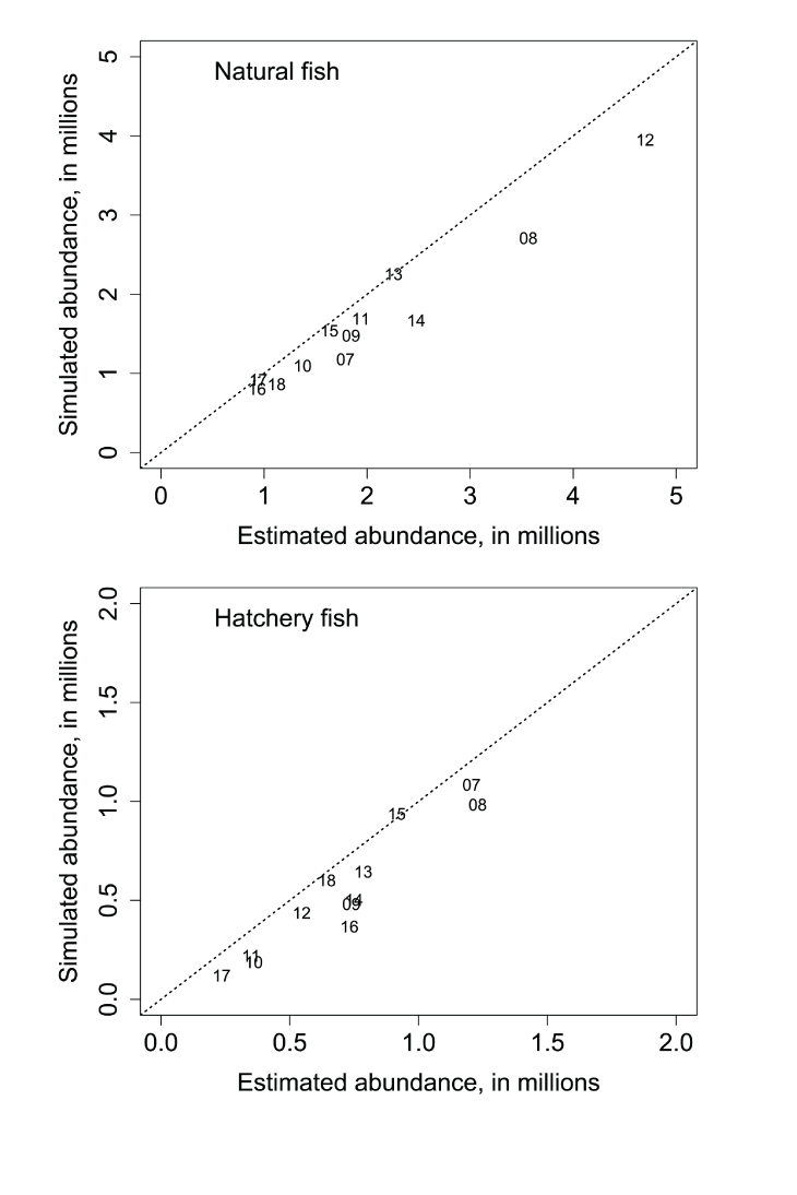
Estimated annual abundance of natural (top) and hatchery (bottom) juvenile Chinook salmon (*Oncorhynchus tshawytscha*) passing the Pear Tree fish trap, Trinity River, California, plotted against their corresponding Stream Salmonid Simulator simulated annual abundances. Data points represent the last two digits of the migration year.

Table 1.

Annual abundances of juvenile Chinook salmon (Oncorhynchus tshawytscha) using the Stream Salmonid Simulator for main stem (natural), tributary (natural), and hatchery source populations as well as annual abundance estimates of natural and hatchery juvenile Chinook salmon estimated to have passed the Pear Tree fish trap on the Trinity River, California.

^{[SD, standard variation]}

Table 1. Annual abundances of juvenile Chinook salmon (Oncorhynchus tshawytscha) using the Stream Salmonid Simulator for main stem (natural), tributary (natural), and hatchery source populations as well as annual abundance estimates of natural and hatchery juvenile Chinook salmon estimated to have passed the Pear Tree fish trap on the Trinity River, California.
Migration year	Simulated main stem abundance	Simulated tributary abundance	Simulated hatchery abundance	Total simulated abundance	Estimated natural abundance	Estimated hatchery abundance	Total estimated abundance
2007	2,096,319	45,926	1,556,949	3,699,194	1,790,174	1,205,522	2,995,696
2008	2,558,604	139,678	983,495	3,681,777	3,564,764	1,229,353	4,794,117
2009	1,421,482	43,696	482,433	1,947,611	1,844,032	738,909	2,582,941
2010	1,042,008	33,714	187,572	1,263,293	1,373,704	359,731	1,733,435
2011	1,603,658	72,505	220,441	1,896,604	1,937,978	348,683	2,286,661
2012	3,829,407	86,629	437,645	4,353,680	4,696,858	545,565	5,242,423
2013	2,102,454	100,249	647,200	2,849,904	2,255,116	785,070	3,040,186
2014	1,555,016	89,929	504,703	2,149,649	2,475,514	749,102	3,224,616
2015	1,460,799	65,958	937,852	2,464,609	1,633,035	914,625	2,547,660
2016	802,319	11,233	368,819	1,182,371	931,634	731,334	1,662,968
2017	901,366	11,655	120,918	1,033,938	943,491	235,051	1,178,542
2018	831,993	14,475	603,339	1,449,806	1,121,302	643,306	1,764,608
Mean	1,683,785	59,637	587,614	2,331,036	2,047,300	707,188	2,754,488
SD	872,957	40,121	407,180	1,102,134	1,112,520	312,730	1,232,117

Figure 2. The time series of estimated weekly abundances and the Stream Salmonid Simulator
simulated weekly abundances of juvenile hatchery and natural Chinook salmon passing
the Pear Tree fish trap each migration year in the Trinity River, California. — Figure 2.
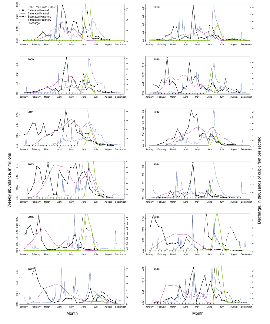
Time series of estimated weekly abundances and the Stream Salmonid Simulator simulated weekly abundances of juvenile hatchery and natural Chinook salmon (*Oncorhynchus tshawytscha*) passing the Pear Tree fish trap each migration year in the Trinity River, California. Also shown is the daily Trinity River discharge (blue line).

Figure 3. The estimated weekly abundance of natural and hatchery juvenile Chinook
salmon plotted against the Stream Salmonid Simulator simulated weekly abundance of
juvenile Chinook salmon passing the Pear Tree fish trap each year in the Trinity River,
California. — Figure 3.
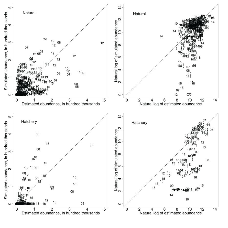
Estimated weekly abundance of natural (top) and hatchery (bottom) juvenile Chinook salmon (*Oncorhynchus tshawytscha*) plotted against the Stream Salmonid Simulator simulated weekly abundance of juvenile Chinook salmon passing the Pear Tree fish trap each year in the Trinity River, California. Data points represent the last two digits of each migration year.

Overall, the S3 model simulated the trend in fish sizes and life-stage transitions over the within year time series (fig. 4). However, we found lack of fit in mean weekly fork lengths in years that showed a marked lack of fit in weekly abundances. For example, in migration year 2017, S3 underestimated the mean weekly size of fish at the trap. Overall, S3 was able to capture the trend in fish growth within each year. Because we fit the S3 model to the time series of abundance and size, improvement in model fit to fish size may best be achieved by matching weekly abundances (figs. 3 and 4).

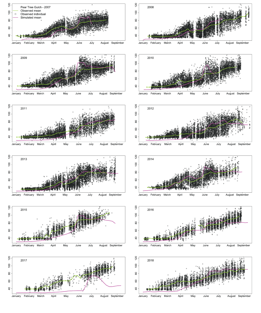
Figure 4. Time series of juvenile Chinook salmon fork lengths at the Pear Tree fish
trap during each migration year. — Figure 4.
Time series of juvenile Chinook salmon (*Oncorhynchus tshawytscha*) fork lengths at the Pear Tree fish trap during each migration year. The black dots are observed fork lengths of individual (hatchery and natural) fish and the green line is the observed mean weekly fork lengths. The mean weekly Stream Salmonid Simulator simulated fork lengths are shown as the magenta line.

Annual Survival, Movement, and Consumption Parameters

Minimizing the EMD with respect to the survival, movement, and consumption parameters to simulate the weekly abundances in each year yielded a best-fit set of S3 parameters for each year (table 1). Annual daily survival probabilities for hatchery fish ranged from S_H_y=0.675 to S_H_y=0.946, with the two lowest S_H_y values associated with wet and dry water year types and annual volumes of water discharged (fig. 5). Using regression, we found no significant trend in S_H_y with higher annual Trinity River water volumes (intercept=0.865, SD=0.055, P<0.0001; slope=-0.0048, SD=0.044, P=0.915; R²=0.001, df=10). Annual daily survival probabilities for natural fish were, on average higher than hatchery fish, and ranged from S_N_y=0.954 to S_N_y=0.984, with an increasing trend in S_N_y during wetter water years and higher annual volumes of water discharged (fig. 5). Consequently, annual survival rates for the simulated hatchery fish were generally lower and more variable than the survival rates simulated for natural fish. A regression of S_N_y on the annual natural Trinity River water volume (in millions of acre feet) discharged showed weak statistical support for an increase in annual fish survival with higher annual water volume (intercept=0.959, SD=0.006, P<0.0001; slope=0.0087, SD=0.0048, P=0.106; R²=0.24, df=10). When the corresponding annual number of spawning females was added to the regression, we found little statistical support for density-dependent effects on S_N_y (slope<0.0001, P=0.77, df=9). To put our average daily survival estimates in perspective, the highest S_N_y=0.984 in 2012 and 2017 results in 85.1 percent of the population surviving after 10 days, whereas the highest S_H_y=0.946 in 2008 results in 57.4 percent of the population surviving after 10d, and the lowest S_H_y=0.675 in 2010 results in 1.9 percent of the population surviving after 10 days. So small differences in daily survival probability can have considerable consequences when integrated over time, and hatchery fish were estimated to have a much lower survival probability compared to natural fish.

Figure 5. Estimates of daily survival probability parameters for hatchery and natural
juvenile Chinook salmon from emergence to the Pear Tree fish trap on the Trinity River,
California. Data points represent the last two digits of the migration year and vertical
dotted lines denote the water year boundary criteria. — Figure 5.
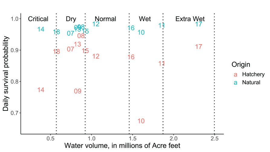
Estimates of daily survival probability parameters for hatchery and natural juvenile Chinook salmon (*Oncorhynchus tshawytscha*) from emergence (or release) to the Pear Tree fish trap on the Trinity River, California. Data points represent the last two digits of the migration year and vertical dotted lines denote the water year boundary criteria.

The intercepts of the Beverton-Holt model for natural, M_0N_y, and hatchery M_0H_y fish represent the probability of remaining in a habitat at low population densities. Over years and fish sources the lowest estimated value was M_0N_y=0.01 in 2017 and the highest value was M_0H_y=0.862 in 2015 (table 2; fig. 6). Higher values M_0N_y or M_0H_y indicate greater potential for density dependent movement over a range in population densities. A multiple regression of M_0N_y on annual discharge volume and the number of spawners showed strong statistical support for both effects. Water volume was the strongest effect (intercept=˗0.128, SD=0.006, P<0.0001; slope=0.2, SD=0.0048, P=0.013; R²=0.67, df=9; fig. 7). On average, M_0N_y were estimated lower (slope-0.190, SD=0.0828, P=0.032) than their corresponding M_0H_y, indicating that hatchery fish were more likely to remain in a habitat at low population densities compared to natural fish (fig. 7).

Table 2.

Estimates of daily survival probability for hatchery (S_H_y) and natural (S_N_y) juvenile Chinook salmon (Oncorhynchus tshawytscha) from emergence (or release) to the Pear Tree fish trap on the Trinity River, California.

^{[Estimates of daily probability of remaining in a habitat unit for hatchery (M_H_y) and natural (M_H_y) juvenile Chinook Salmon, the daily consumption rate (C_y), the water year type and total volume discharged during the juvenile migration year,
and the corresponding total number of spawners during the previous brood year. Ext,
extremely; SD, standard deviation; --, not applicable]}

Table 2. Estimates of daily survival probability for hatchery (SHy) and natural (SNy) juvenile Chinook salmon (Oncorhynchus tshawytscha) from emergence (or release) to the Pear Tree fish trap on the Trinity River, California.
Migration year	S_H_y	S_N_y	M_H_y	M_N_y	C_y	Water year type	Water volume (millions of acre feet)	Spawners
2007	0.904	0.954	0.089	0.108	0.783	Dry	0.745	3,359
2008	0.946	0.974	0.238	0.244	0.761	Dry	0.871	4,794
2009	0.770	0.972	0.769	0.237	0.772	Dry	0.831	2,662
2010	0.675	0.957	0.748	0.257	0.750	Wet	1.602	3,098
2011	0.858	0.979	0.413	0.401	0.600	Wet	1.855	2,987
2012	0.881	0.984	0.353	0.352	0.656	Normal	1.051	4,564
2013	0.919	0.967	0.436	0.676	0.585	Dry	0.827	11,494
2014	0.774	0.967	0.285	0.218	0.887	Critical	0.381	2,163
2015	0.898	0.960	0.862	0.010	0.357	Dry	0.922	3,841
2016	0.879	0.971	0.382	0.366	0.627	Wet	1.479	1,414
2017	0.911	0.983	0.630	0.440	0.278	Ext Wet	2.304	1,478
2018	0.896	0.959	0.398	0.010	0.629	Critical	0.571	1,535
Mean	0.859	0.969	0.467	0.277	0.640	--	1.120	3,616
SD	0.079	0.010	0.235	0.189	0.176	--	0.569	2,729

Figure 6. Beverton-Holt model relationships for the daily probability of moving from
a habitat over a range in fish densities. — Figure 6.
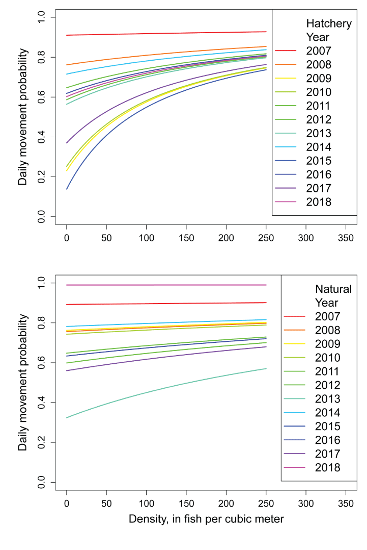
Beverton-Holt model relationships for the daily probability of moving from a habitat over a range in fish densities. Estimates are provided for hatchery (top) and natural (bottom) juvenile Chinook salmon (*Oncorhynchus tshawytscha*) in the restoration reach of the Trinity River, California.

Figure 7. Estimates of the intercept for the Beverton-Holt model representing the
daily probability of remaining in a habitat at near-zero abundance and fish densities.
Estimates are provided for hatchery and natural juvenile Chinook salmon from emergence
to the Pear Tree fish trap on the Trinity River, California. Data points represent
the last two digits of the migration year and vertical dotted lines denote the water
year boundary criteria. — Figure 7.
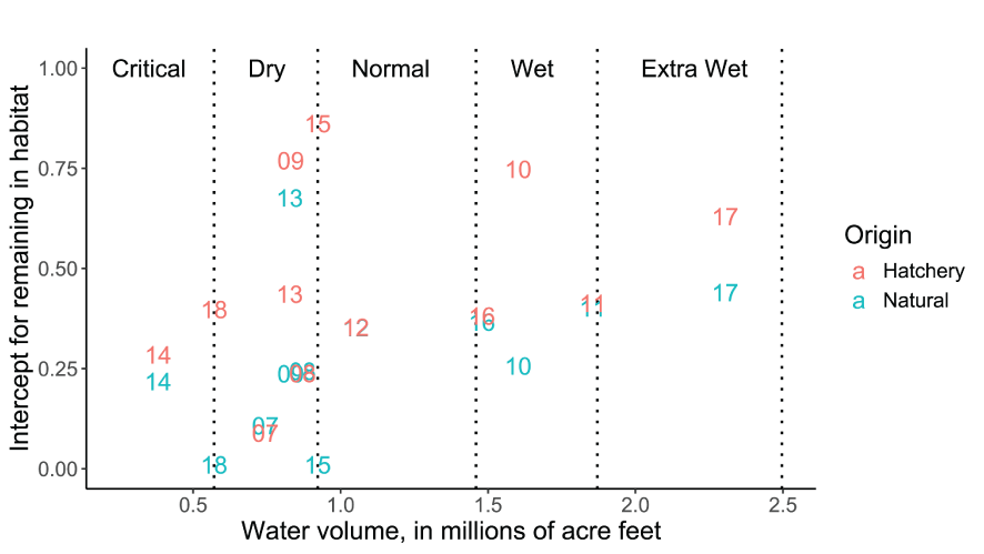
Estimates of the intercept for the Beverton-Holt model representing the daily probability of remaining in a habitat at near-zero abundance and fish densities. Estimates are provided for hatchery and natural juvenile Chinook salmon (*Oncorhynchus tshawytscha*) from emergence (or release) to the Pear Tree fish trap on the Trinity River, California. Data points represent the last two digits of the migration year and vertical dotted lines denote the water year boundary criteria.

On average, the overall proportion of maximum consumption across all study years was $\bar{C}$ =0.64 (SD=0.176) indicating that the assumed value of $\bar{C}$ =0.66 used in past S3 calibrations and simulations was accurate. However, estimated mean annual proportions of maximum consumption were highly variable over the years ranging from C_y=0.278 to C_y=0.887. A regression of C_y on the total annual water volume discharged indicated that during critical dry conditions (for example, 2014; SD=0.099, P<0.0001; slope=-0.179, SD=0.0798, P=0.049; R²=0.33, df=10) lower consumption relative to the fish’s expected maximum consumption might be expected (table 2; fig. 8). However, this relation was largely driven by the critically dry and extremely wet years of 2014 and 2017, respectively. Thus, in wetter years natural fish were estimated to generally survive at higher rates, move less (at low fish abundance), and consume less relative to expected maximum consumption.

Figure 8. Estimates of mean daily proportions or maximum consumption for juvenile
Chinook salmon from emergence to the Pear Tree fish trap on the Trinity River, California.
Data points represent the last two digits of the migration year and vertical dotted
lines denote the water year boundary criteria. — Figure 8.
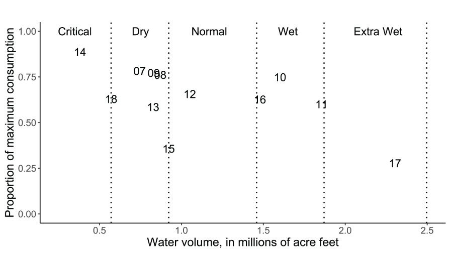
Estimates of mean daily proportions or maximum consumption for juvenile Chinook salmon (*Oncorhynchus tshawytscha*) from emergence (or release) to the Pear Tree fish trap on the Trinity River, California. Data points represent the last two digits of the migration year and vertical dotted lines denote the water year boundary criteria.

Annual S3 Model Output

Annual summaries of the S3 output demonstrate differences in survival, biomass, and size among the source populations and years from egg incubation to migration past the Pear Tree fish trap (tables 3–5). For example, annual egg survival rates ranged from 0.612 to 0.751. A log-to-log regression of egg survival on the number of spawners explained most of this variation (R²=0.668) with higher spawner abundance associated with lower egg survival (fig. 9; table 3), indicating redd superimposition as a primary cause for lower egg survival, and in part, density dependence in the production of juveniles at the Pear Tree fish trap. Survival of juvenile fish from emergence to the Pear Tree fish trap ranged from 0.114 to 0.398 for natural fish in the main stem and ranged from 0.103 to 0.524 for hatchery fish. On average, the annual survival of hatchery fish from release to the Pear Tree fish trap (0.215; SD=0.142) was slightly lower and more variable than the overall annual survival of natural fish (0.241; SD=0.080) from the main stem Trinity River. Because of their closer proximity to the Pear Tree fish trap site (9.3 kilometers), tributary fish entering the Trinity River from Canyon Creek had higher average annual survival (0.791; SD=0.067) to the Pear Tree fish trap site than fish from main stem and hatchery source populations.

Table 3.

Simulated annual survival of juvenile Chinook salmon (Oncorhynchus tshawytscha) from emergence to passage at the Pear Tree fish trap using the Stream Salmonid Simulator for main stem (natural), tributary (natural), and hatchery source populations in the Trinity River, California.

^{[Water year type and total volume during the juvenile migration year, and the corresponding
total number of spawners during the previous brood year. Ext, extremely; SD, standard
deviation; --, not applicable]}

Table 3. Simulated annual survival of juvenile Chinook salmon (Oncorhynchus tshawytscha) from emergence to passage at the Pear Tree fish trap using the Stream Salmonid Simulator for main stem (natural), tributary (natural), and hatchery source populations in the Trinity River, California.
Migration year	Egg survival rate	Main stem juvenile survival	Tributary juvenile survival	Hatchery juvenile survival	Water year type	Water volume (millions of acre feet)	Spawners
2007	0.679	0.293	0.833	0.524	Dry	0.745	3359
2008	0.650	0.262	0.828	0.387	Dry	0.871	4794
2009	0.722	0.236	0.821	0.159	Dry	0.831	2662
2010	0.727	0.148	0.721	0.070	Wet	1.602	3098
2011	0.712	0.241	0.812	0.082	Wet	1.855	2987
2012	0.673	0.398	0.864	0.163	Normal	1.051	4564
2013	0.612	0.095	0.611	0.227	Dry	0.827	11494
2014	0.736	0.312	0.805	0.156	Critical	0.381	2163
2015	0.751	0.161	0.796	0.383	Dry	0.922	3841
2016	0.744	0.243	0.778	0.123	Wet	1.479	1414
2017	0.734	0.265	0.829	0.103	Ext Wet	2.304	1478
2018	0.726	0.238	0.794	0.205	Critical	0.571	1535
Mean	0.705	0.241	0.791	0.215	--	1.120	3,616
SD	0.043	0.080	0.067	0.142	--	0.569	2,729

Table 4.

Mean annual mass (in grams) of juvenile Chinook salmon (Oncorhynchus tshawytscha) using the Stream Salmonid Simulator for spring and fall stocks from main stem (natural), tributary (natural), and hatchery source populations that passed the Pear Tree fish trap on the Trinity River, California.

^{[SD, standard deviation]}

Table 4. Mean annual mass (in grams) of juvenile Chinook salmon (Oncorhynchus tshawytscha) using the Stream Salmonid Simulator for spring and fall stocks from main stem (natural), tributary (natural), and hatchery source populations that passed the Pear Tree fish trap on the Trinity River, California.
Migration year	Spring hatchery	Fall hatchery	Tributary	Spring main stem	Fall main stem
2007	5.81	3.74	1.62	0.54	0.85
2008	6.17	4.42	1.74	1.28	1.84
2009	10.85	7.79	1.83	0.97	2.14
2010	9.60	5.48	1.70	0.58	1.10
2011	6.88	4.88	1.64	0.74	1.71
2012	7.59	4.62	1.70	1.00	2.11
2013	7.29	4.93	2.16	1.27	3.20
2014	8.88	6.48	2.03	0.93	2.54
2015	9.87	7.58	1.55	0.41	0.69
2016	5.96	5.12	1.82	0.79	1.59
2017	5.22	3.21	1.43	0.33	0.44
2018	7.49	5.96	1.70	0.50	1.30
Mean	7.63	5.35	1.74	0.78	1.63
SD	1.80	1.40	0.20	0.32	0.81

Table 5.

Mean annual biomass (metric tons) of juvenile Chinook salmon (Oncorhynchus tshawytscha) using the Stream Salmonid Simulator for spring and fall stocks from main stem (natural), tributary (natural), and hatchery source populations that passed the Pear Tree fish trap on the Trinity River, California.

^{[SD, standard deviation]}

Table 5. Mean annual biomass (metric tons) of juvenile Chinook salmon (Oncorhynchus tshawytscha) using the Stream Salmonid Simulator for spring and fall stocks from main stem (natural), tributary (natural), and hatchery source populations that passed the Pear Tree fish trap on the Trinity River, California.
Migration year	Spring hatchery	Fall hatchery	Tributary	Spring main stem	Fall main stem
2007	3.611	3.495	0.003	0.679	0.710
2008	2.260	2.727	0.017	1.568	2.464
2009	4.757	0.341	0.009	0.827	1.210
2010	1.797	0.002	0.002	0.410	0.362
2011	0.764	0.534	0.020	0.813	0.869
2012	2.070	0.761	0.010	2.509	2.780
2013	2.794	1.300	0.005	1.980	1.754
2014	3.547	0.681	0.021	1.162	0.792
2015	7.119	1.643	0.002	0.464	0.230
2016	1.000	1.029	0.002	0.569	0.137
2017	0.627	0.002	0.002	0.279	0.021
2018	2.156	1.878	0.001	0.317	0.249
Mean	2.71	1.20	0.09	0.96	0.96
SD	1.86	1.08	0.07	0.71	0.92

Figure 9. Simulated egg survival rate and main stem natural production of juvenile
Chinook salmon passing the Pear Tree fish trap on the Trinity River, California as
a function of the estimated number of female spawners that were used as input data
for the Stream Salmonid Simulator. — Figure 9.
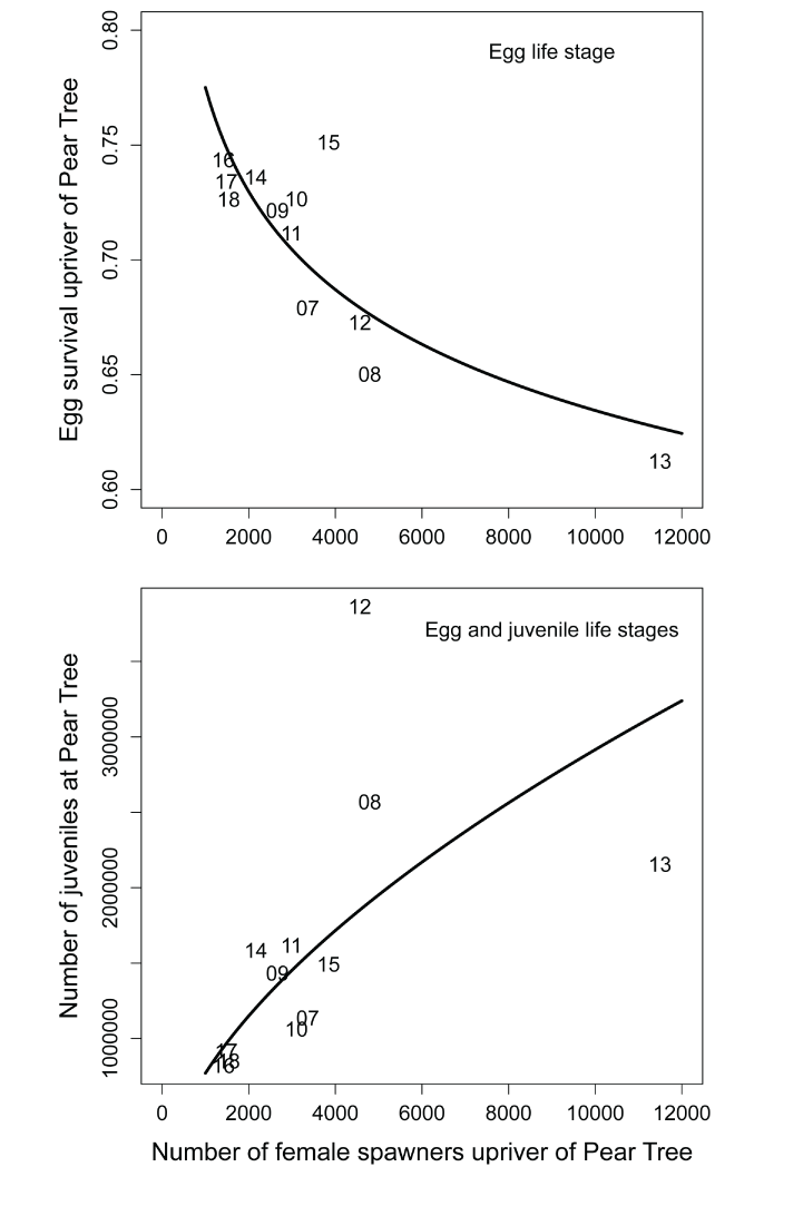
Simulated egg survival rate (top) and main stem natural production of juvenile Chinook salmon (*Oncorhynchus tshawytscha*) passing the Pear Tree fish trap (bottom) on the Trinity River, California as a function of the estimated number of female spawners that were used as input data for the Stream Salmonid Simulator. Data points are represented by the last two digits of each migration year and regression lines are the log-to-log relation.

Differences in mean annual fish size among the source populations reflected the initial fish size of the source population, their travel time to Pear Tree, and the estimated consumption rate C_y (table 4). Overall mean annual size of simulated fish was 7.6 g (SD=1.8) for hatchery spring run Chinook salmon and 5.3 g (SD=1.4) for hatchery fall run Chinook salmon. The overall mean annual size of simulated fish (spring and fall run) from the Canyon Creek tributary was 1.7 g (SD=0.20) at the Pear Tree fish trap. Simulated fish that emerged in the main stem Trinity River had an overall mean annual size of 0.78 g (SD=0.32) for spring and 1.63 g (SD=0.81) for fall run Chinook salmon.

Total annual biomass reflects the differences in annual abundance and mean annual fish size among the source populations (table 5). Overall mean biomass for simulated hatchery fish ranged 2.71 metric tons (SD=1.86) for spring run to 1.20 metric tons (SD=1.08) for fall run juvenile Chinook salmon. Overall mean biomass for natural fish of spring and fall run were similar (mean=0.96), but annual biomass between spring and fall stocks was highly variable ranging from 0.002 to 7.1 metric tons of juvenile fish. Hatchery fish represented 66 percent of the total biomass of fish that passed the Pear Tree fish trap.

Discussion

We constructed and parameterized the S3 fish production model to support the Trinity River restoration efforts and decision support system. The structure of the S3 model allows for the assessment of hypothesized management actions because the model is sensitive to (1) water temperature, (2) daily discharge management, and (3) the resulting changes in habitat quality and quantity. Each of these variables are key management parameters under consideration in the Trinity River and other river systems. Furthermore, the Trinity River S3 model is novel among detailed simulation models of fish populations because of (1) state-of-the-art sub-models forming key drivers in S3 (for example, hydrodynamics and fish habitat models), (2) high-quality abundance estimates available for evaluating model output, (3) calibration of the model to estimate key demographic parameters, and (4) the potential to compare alternative hypotheses and improve our understanding of the mechanisms driving salmon population dynamics.

This report is an extension to previous S3 modeling efforts (Perry and others 2018c) by estimating consumption as well as annual movement and survival parameters. We fit the model to individual years of weekly trap abundance estimates and used a different parameter optimization method that could accommodate multivariate data on abundance and fish size at the Pear Tree fish trap. This approach demonstrated the year-to-year variability in estimates of survival, movement, and consumption, and in part, year-specific conditions helped explain the interannual variability among S3 model parameters.

Calibration of the S3 model on an annual basis facilitates identification of potential causes for lack of model fit. Three factors likely contributed to a lack of fit. First, from 2015 to 2017 trapping efforts started later in the year and missed the early portion of the juvenile salmon outmigration. So, the total annual abundance estimate is likely negatively biased, and it affected model calibration and fit. Second, the trap abundance estimates themselves may be biased due to size selectivity in trap efficiency. Size selectivity is apparent in figure 4 where the average size early in the year is approximately 40 mm, indicating that the trap was not capturing smaller fish, and because we used fish size to calculate the EMD, size selectivity by the fish trap affected model calibration and potentially the fit to abundance. Third, the S3 model may not be incorporating some early life-stage dynamics such as spawn timing, tributary juveniles, or egg development in the main stem Trinity River. Thus, gain in the fit and predictive accuracy of S3 may be achieved by identifying the factors that affect fish trap abundance estimates and S3 simulations.

Caution should be used when making inferences across the annual S3 parameter estimates in relation to spawner abundances, water year types and volumes. The parameters obtained by fitting S3 simulations to trap abundances and fish sizes is an indirect approach to estimating survival, movement, and consumption parameters for juvenile salmon populations. We identified patterns over the annual parameter values, water year types, and annual Trinity River volumes. The most outlying parameter estimates for natural fish in the Trinity River were during the high discharge year of 2017. In this year we estimated high fish survival with S_N_y=0.983 in 2017, a high intercept on fish movement relative to other years with M_0N_y=0.440, and the lowest estimate across years for fish consumption. The poorest fit to the fish size and abundance data was in this year, suggesting incongruence between S3 and the abundance and size of fish estimated at the trap during the high discharge year of 2017. Nonetheless, regressions of S_N_y, M_0N_y, and C_y indicated trends in annual S3 parameter estimates in association with annual conditions such as the total water volume. The data suggest an increase in S_N_y and M_0N_y as the total annual water volume for the Trinity River increased, suggesting greater survival and higher site fidelity at low population densities with increased discharge. Values for C_y over the range of discharges should be interpreted cautiously because relationships were largely driven by just two data points at extreme high and low discharge volumes.

Proportions of maximum consumption were generally quite high (table 1), and on average, the fish caught by the juvenile trap were feeding at average consumption rates (mean=0.640, SD=0.176) that were very similar to what has been assumed in past S3 calibration and simulations (Perry and others, 2018a,b; Plumb and others, 2023). Past S3 calibration and applications assumed an average fixed value of ${\bar{C}}_{}$ =0.66, and the independent estimates of C_y reported here support the assumption of earlier S3 calibrations and evaluations. This finding suggests that the fish were eating at about two thirds of maximum consumption, which is approximately the digestive capacity reported by other studies that have estimated $\bar{C}$ for juvenile salmon (Armstrong and Schindler, 2011).

This report represents the third iteration of using the S3 model as a framework for research and management of the Trinity River, and with each iteration we learn more about the S3 model’s limitations and strengths. The S3 model offers the opportunity to integrate biological and physical characteristics over the entire temporal and spatial freshwater residency of juvenile salmonid populations. As such, the S3 model can provide valuable insights into the potentially variable effects that different management decisions may have on the restoration reach of the Trinity River. Combinations of system attributes (for example, physical habitat, hydrographs, and temperatures) subject to manipulation by managers can be translated into scenarios that form the inputs for S3 model runs. The S3 model has the potential to (1) provide more accurate predictions of absolute abundance by estimating life-stage-specific abundances at the traps, incorporating information from independent studies on egg or juvenile survival and migration rates, and (2) further model development and hypothesis testing to determine variables important to juvenile salmon during their outmigration. Currently (2024), S3 model output maybe useful when comparing relative differences of population demographics such as fish abundance, size, and run timing across pre-specified scenarios. These predictions may inform a broader management objective (as well as model development), and in turn, complete the adaptive management loop, leading to a refined management decision process for the benefit of the Trinity River.

References Cited

Aggarwal, C.C., Hinneburg, A., and Keim, D.A., 2001, On the surprising behavior of distance metrics in high dimensional space, in Van den Bussche, J., and Vianu, V., eds., Database theory—ICDT 2001: Berlin, Springer, v. 1973, p. 420–434.

Armstrong, J., and Schindler, D., 2011, Excess digestive capacity in predators reflects a life of feast and famine: Nature, v. 476, no. 7358, p. 84–87, accessed July 2013, at https://doi.org/10.1038/nature10240.

Bradley, D.N., 2016, Trinity River 40 Mile Hydraulic Model—Development and analysis. Report to the Trinity River Restoration Program (TRRP): Denver, Colorado, U.S. Bureau of Reclamation, Technical Service Center report no. SRH-2016-27, 46 p. https://www.trrp.net/library/document/?id=2297.

Buffington, J., Jordan, C., Merigliano, M., Peterson, J., and Stalnaker, C., 2014, Review of the Trinity River Restoration Program following Phase 1, with emphasis on the Program’s channel rehabilitation strategy: Arcata, California, Trinity River Restoration Program, prepared by the Trinity River Restoration Program’s Science Advisory Board, Anchor QEA. LLC, Stillwater Sciences, BioAnalysts, Inc., and Hinrichsen Environmental Services, 52 p.

Chamberlain, C.D., Quinn, S., and Matilton, W., 2012, Distribution and abundance of Chinook salmon redds in the mainstem Trinity River 2002 to 2011: Arcata, California, U.S. Fish and Wildlife Service, Arcata Fisheries Technical Report TR 2012-16, 46 p.

ESRI 2011. ArcGIS Desktop: Release 10. 6, Redlands, CA: Environmental Systems Research Institute.

Geist, D.R., Abernethy, S.C., Hand, K.D., Cullinan, V.I., Chandler, J.A., and Groves, P.A., 2006, Survival, development, and growth of fall Chinook salmon embryos, alevins, and fry exposed to variable thermal and dissolved oxygen regimes: Transactions of the American Fisheries Society, v. 135, no. 6, p. 1462–1477.

Gough, S.A., Som, N.A., Quinn, S., Matilton, W.C., Hill, A.M., and Brock, W., 2019, Mainstem Trinity River Chinook salmon spawning survey, 2017: Arcata, California, U.S. Fish and Wildlife Service, Report DS 2019-62, 50 p. [Also available at https://www.trrp.net/library/document?id=2558.]

Gough, S.A., Som, N.A., Laskodi, C., Matilton, B.C., Hill, A.M., and Fleitz, A., 2021, Mainstem Trinity River Chinook Salmon Spawning Survey, 2018: Arcata, California, U.S. Fish and Wildlife Service, Report DS 2021-65, 50 p. [Also available at https://www.trrp.net/library/document?id=2559.]

Jones, E.C., Perry, R.W., Risley, J.C., Som, N.A., and Hetrick, N.J., 2016, Construction, calibration, and validation of the RBM10 water temperature model for the Trinity River, northern California: U.S. Geological Survey Open-File Report 2016–1056, 46 p., accessed October 1, 2018, at https://doi.org/10.3133/ofr20161056.

Levina, E., and Bickel, P., 2001, The Earth mover’s distance is the mallows distance: some insights from statistics: Proceedings Eighth Institute of Electronics and Electronic Engineers, International Conference on Computer Vision 2001, p. 251–256, accessed January 2020, at https://doi.org/10.1109/ICCV.2001.937632.

Ling, H., and Okada, K., 2007, An efficient Earth mover’s distance algorithm for robust histogram comparison: IEEE Transactions on Pattern Analysis and Machine Intelligence, v. 29, no. 5, p. 840–853.

Lupu, N., Selios, L., and Warner, Z., 2017, A new measure of congruence—The earth mover’s distance: Political Analysis, v. 25, no. 1, p. 95–113, accessed January 2020, at https://doi.org/10.1017/pan.2017.2.

Manhard, C.V., Som, N.A., Perry, R.W., and Plumb, J.M., 2018, A laboratory calibrated model of coho salmon growth with utility for ecological analyses: Canadian Journal of Fisheries and Aquatic Sciences, v. 75, no. 5, p. 682–690, accessed October 1, 2018, at https://doi.org/10.1139/cjfas-2016-0506.

Perry, R.W., Risley, J.C., Brewer, S.J., Jones, E.C., and Rondorf, D.W., 2011, Simulating daily water temperatures of the Klamath River under dam removal and climate change scenarios: U.S. Geological Survey Open-File Report 2011–1243, 78 p.

Perry, R.W., Plumb, J.M., and Huntington, C.W., 2015, Using a laboratory-based growth model to estimate mass-and temperature-dependent growth parameters across populations of juvenile Chinook Salmon: Transactions of the American Fisheries Society, v. 144, no. 2, p. 331–336.

Perry, R.W., Plumb, J.M., Jones, E.C., Som, N.A., Hetrick, N.J., and Hardy, T.B., 2018a, Model structure of the Stream Salmonid Simulator (S3)—A dynamic model for simulating growth, movement, and survival of juvenile salmonids: U.S. Geological Survey Open-File Report 2018–1056, 32 p. [Also available at https://doi.org/10.3133/ofr20181056.]

Perry, R.W., Plumb, J.M., Jones, E.C., Som, N.A., Hetrick, N.J., and Hardy, T.B., 2018b, Application of the Stream Salmonid Simulator (S3) to Klamath River fall Chinook salmon: U.S. Geological Survey Open-File Report 2018–1056, 32 p.

Perry, R.W., Jones, E.C., Plumb, J.M., Som, N.A., Hetrick, N.J., Hardy, T.B., Polos, J.C., Martin, A.C., Alvarez, J.S., and De Juilio, K.P., 2018c, Application of the Stream Salmonid Simulator (S3) to the restoration reach of the Trinity River, California—Parameterization and calibration: U.S. Geological Survey Open-File Report 2018–1174, 64 p.

Pinnix, W.D., Boyle, S.P., Wallin, T., Daley, T., and Som, N.A., 2022, Long-term analyses of estimates of abundance of juvenile Chinook salmon on the Trinity River, 1989–2018: Arcata, California, U.S. Fish and Wildlife Service Arcata Fisheries Technical Series Report TS 2022-40, 90 p. [Also available at https://www.trrp.net/library/document?id=2571.]

Plumb, J.M., Perry, R.W., Som, N.A., Goodman, D.H., Martin, A.C., Alvarez, J.S., and Hetrick, N.J., 2023, Calibration of the Trinity River Stream Salmonid Simulator (S3) with extension to the Klamath River, California, 2006–17: U.S. Geological Survey Open-File Report 2023–1023 54 p.

Plumb, J.M., Perry, R.W., Som, N.A., Alexander, J., and Hetrick, N.J., 2019, Using the stream salmonid simulator (S3) to assess juvenile Chinook Salmon (Oncorhynchus tshawytscha) production under historical and proposed action flows in the Klamath River, California: U.S. Geological Survey Open-File Report 2019–1099, 43 p. [Also available at https://doi.org/10.3133/ofr20191099.]

Plumb, J.M., and Moffitt, C.M., 2015, Re-estimating temperature-dependent consumption parameters in bioenergetics models for juvenile Chinook Salmon: Transactions of the American Fisheries Society, v. 144, no. 2, p. 323–330.

Plumb, J.M., 2012, Evaluation of models and the factors affecting the migration and growth of naturally-produced subyearling fall Chinook salmon (Oncorhynchus tshawytscha) in the lower Snake River: Moscow, Idaho, University of Idaho, PhD dissertation, 153 p.

R Core Team, 2022, R—A language and environment for statistical computing version 4.2.2 (Innocent and Trusting): Vienna, Austria, R Foundation for Statistical Computing software release, accessed October 31, 2022, at https://www.R-project.org/.

Rupert, D.L., Chamberlain, C.D., Gough, S.A., Som, N.A., Davids, N.J., Matilton, B.C., Hill, A.M., and Wiseman, E.R., 2017a, Mainstem Trinity River Chinook salmon spawning distribution 2012–2014: Arcata, California, U.S. Fish and Wildlife Service, Arcata Fish and Wildlife Office, Arcata Fisheries Data Series Report Number DS 2017–52, 86 p. [Also available at https://www.trrp.net/library/document?id=2321.]

Rupert, D.L., Gough, S.A., Som, N.A., Davids, N.J., Matilton, B.C., Hill, A.M., and Pabich, J.L., 2017b, Mainstem Trinity River chinook salmon spawning survey, 2015 and 2016: Arcata, California, U.S. Fish and Wildlife Service, Arcata Fisheries Data Series Report Number DS 2017–56, 53 p. [Also available at https://www.trrp.net/library/document?id=2344.]

Stewart, D. J., and Ibarra, M., 1991, Predation and production of salmonine fishes in Lake Michigan, 1978–88: Canadian Journal of Fisheries and Aquatic Sciences v. 48, no. 5, p. 909–922.

Som, N.A., Perry, R.W., Jones, E.C., De Juilio, K., Petros, P., Pinnix, W.D., and Rupert, D.L., 2018a, N-mix for fish—Estimating riverine salmonid habitat selection via N-mixture models: Canadian Journal of Fisheries and Aquatic Sciences, v. 75, no. 7, p. 1048–1058, accessed January 2019, at https://www.nrcresearchpress.com/doi/10.1139/cjfas-2017-0027.

Som, N.A., Alvarez, J., and Martin, A., 2018b, Assessment of Chinook salmon smolt habitat use in the lower Trinity River: Arcata, California Hoopa Valley Tribal Fisheries Department, Yurok Tribal Fisheries Program, and U.S. Fish and Wildlife Service, Arcata Fish and Wildlife Office, Arcata Fisheries Data Series Report Number DS 2018-57, 11 p.

Trinity River Restoration Program and ESSA Technologies, Ltd., 2009, Integrated assessment plan, version 1.0—September 2009: Weaverville, California, Trinity River Restoration Program, 285 p.

U.S. Department of the Interior, 2000, Record of decision—Trinity River mainstem fishery restoration final environmental impact statement/environmental impact report, December 2000: U.S. Department of the Interior, accessed July 2013, at https://www.trrp.net/program-structure/background/rod/.

Urbanek, S. and Rubner, Y., 2022, Earth Mover’s Distance, An R function, version 3.1., R Foundation for Statistical Computing, accessed October 31, 2022, at https://www.R-project.org/.

Zabel, R.W., and Anderson, J.J., 1997, A model of the travel time of migrating juvenile salmon, with an application to Snake River Spring Chinook Salmon: North American Journal of Fisheries Management, v. 17, no. 1, p. 93–100.

Zabel, R.W., 2002, Using “travel time” data to characterize the behavior of migrating animals: American Naturalist, v. 159, no. 4, p. 372–387.

Conversion Factors

U.S. customary units to International System of Units


Multiply	By	To obtain
Flow rate
cubic foot per second (ft³/s)	0.02832	cubic meter per second (m³/s)

International System of Units to U.S. customary units


Multiply	By	To obtain
Length
centimeter (cm)	0.3937	inch (in.)
millimeter (mm)	0.03937	inch (in.)
meter (m)	1.094	yard (yd)
kilometer (km)	0.3107	mile (mi)
Volume
cubic meter (m³)	264.2	gallon (gal)
cubic decimeter (dm³)	0.03531	cubic foot (ft³)
acre-foot	1,233.48	cubic meters (m³)
Mass
gram (g)	0.03527	ounce, avoirdupois (oz)
metric ton	2,204.6	pounds (lbs)
Area
square meter (m2)	0.0002471	acre
hectare (ha)	2.471	acre
hectare (ha)	0.003861	square mile (mi2)

Temperature in degrees Celsius (°C) may be converted to degrees Fahrenheit (°F) as follows:

°F = (1.8 × °C) + 32.

Abbreviations

DSS: Decision Support System
EMD: Earth Mover’s Distance
FL: fork length
MHU: meso-habitat unit
S3: Stream Salmon Simulator
SD: standard deviation
TRRP: Trinity River Restoration Program
USGS: U.S. Geological Survey

For information about the research in this report, contact:

Director, Western Fisheries Research Center

U.S. Geological Survey

6505 NE 65th Street

Seattle, Washington 98115-5016

https://www.usgs.gov/centers/wfrc

Manuscript approved on November 9, 2023

Publishing support provided by the U.S. Geological Survey

Science Publishing Network, Tacoma Publishing Service Center

Disclaimers

Any use of trade, firm, or product names is for descriptive purposes only and does not imply endorsement by the U.S. Government.

Although this information product, for the most part, is in the public domain, it also may contain copyrighted materials as noted in the text. Permission to reproduce copyrighted items must be secured from the copyright owner.

Suggested Citation

Plumb, J.M., Perry, R.W., and De Juilio, K., 2025, Calibration of the Stream Salmonid Simulator (S3) model to estimate annual survival, movement, and food consumption by juvenile Chinook salmon (Oncorhynchus tshawytscha) in the restoration reach of the Trinity River, California, 2006–18: U.S. Geological Survey Open-File Report 2024–1070, 21 p., https://doi.org/10.3133/ofr20241070.

ISSN: 2331-1258 (online)

Study Area

Additional publication details
Publication type	Report
Publication Subtype	USGS Numbered Series
Title	Calibration of the Stream Salmonid Simulator (S3) model to estimate annual survival, movement, and food consumption by juvenile Chinook salmon (Oncorhynchus tshawytscha) in the restoration reach of the Trinity River, California, 2006–18
Series title	Open-File Report
Series number	2024-1070
DOI	10.3133/ofr20241070
Publication Date	May 15, 2025
Year Published	2025
Language	English
Publisher	U.S. Geological Survey
Publisher location	Reston, VA
Contributing office(s)	Western Fisheries Research Center
Description	vii, 22 p.
Country	United States
State	California
Online Only (Y/N)	Y