

Mapping Eelgrass (Zostera marina) Cover and Biomass at Izembek Lagoon, Alaska, Using In-Situ Field Data and Sentinel-2 Satellite Imagery
Links
- Document: Report (10.1 MB pdf) , HTML , XML
- Data Release: USGS data release - Eelgrass (Zostera marina) maps from 2016 and 2020, at Izembek Lagoon, Alaska
- Superseded Publications:
- Download citation as: RIS | Dublin Core
Acknowledgments
We authors thank the European Space Agency and the Copernicus Data Space Ecosystem for making Sentinel-2 data available to the scientific community (https://dataspace.copernicus.eu). We used imagery from the National Aeronautics and Space Administration (NASA) Worldview application (https://worldview.earthdata.nasa.gov), part of the NASA Earth Science Data and Information System.
Abstract
The U.S. Geological Survey and the U.S. Fish and Wildlife Service have developed a three-tiered strategy for monitoring eelgrass (Zostera marina) beds at Izembek Lagoon, Alaska, that targets different spatial and temporal scales. The broadest-scale monitoring (tier-1) uses satellite imagery about every 5 years to delineate the spatial extent of eelgrass beds throughout the lagoon. This report describes the most recent (mid-2020s) tier-1 eelgrass monitoring at Izembek Lagoon. The monitoring effort began by canvasing all satellite imagery collected during summer, under clear daytime skies and at low-tide, since the last tier-1 effort in 2006. Two eelgrass maps of Izembek Lagoon were generated by first creating maps of spectrally unique classes from two Sentinel-2 satellite images collected on July 1, 2016, and August 14, 2020, then attributing those spectral classes with information about eelgrass conditions based on field data. Specifically, maps depicting various eelgrass metrics, such as percentage of cover and modeled biomass, were generated using summaries of the ground data that spatially intersected each spectral class. Comparisons of the 2016 and 2020 Sentinel-2 maps showing eelgrass distributional extent, as well as a 2006 Landsat map, indicated that areas where eelgrass presence may have declined during 2006–20 were most prevalent in the central part of Izembek Lagoon. More recently, during 2016-20, areas of possible biomass decline were more prevalent in the southern part of the lagoon. Monitoring eelgrass conditions at Izembek Lagoon with satellite imagery and concurrent ground data allows conditions to be compared over time, but the influences of tide levels, growing season phenology, and spatiotemporal co-registration accuracy should be considered when designing and interpreting change detection analyses.
Introduction
Izembek Lagoon is a large shallow embayment (about 50 kilometers [km] long by 10 km wide) on the Bering Sea side of the Alaska Peninsula within the Izembek National Wildlife Refuge and Izembek State Game Refuge. Maximum tidal ranges in the embayment are modest (about 1 meter [m]), waters are generally clear, salinity ranges from about 26 parts per thousand to 32 parts per thousand (McRoy, 1966), and the maritime climate is cool (mean monthly air temperatures range from −2 to 11 degrees Celsius annually [Brower and others 1988]). Storms are common throughout the year, and ice cover forms intermittently from December to March (McRoy, 1966). The lagoon is dominated by broad tidal flats interspersed with networks of channels stemming from the lagoon’s three entrances at the northern, central, and southern ends. Eelgrass (Zostera marina) is the predominant submerged aquatic vegetation. More about the physical and biological environment at Izembek Lagoon can be found in Ward and others (1997).
Izembek Lagoon supports one of the largest eelgrass beds in the world (McRoy, 1966), lending to its designation as a wetland of international importance (Ramsar, 2023). Eelgrass provides a key source of nutrients for the lagoon’s food web, which includes numerous species of birds, fish, and marine mammals (Ward and others, 1997). Owing to (1) the importance of Izembek Lagoon ecologically, (2) the growing threats to eelgrass along the United States (U.S.) mainland Pacific Coast (Sherman and DeBruyckere, 2018), and (3) recent environmental changes in the Bering Sea (Wood and others, 2015; Overland and others, 2024), the U.S. Geological Survey and the U.S. Fish and Wildlife Service have developed a 3-tiered strategy for monitoring eelgrass beds at Izembek that targets different spatial and temporal scales (Neckles and others, 2012; Hogrefe and others, 2014; Ward and Amundson, 2019). The broadest-scale monitoring effort (tier-1) uses satellite imagery about every 5 years to delineate the spatial extent of eelgrass beds throughout the lagoon.
This report describes the most recent (mid-2020s) tier-1 eelgrass monitoring at Izembek Lagoon. Two suites of eelgrass maps were created using Sentinel-2 satellite imagery (Phiri and others, 2020) collected in 2016 and 2020. We applied unsupervised (mathematical only) spectral classification techniques to the imagery and then used field data (Ward, 2021) to quantitatively attribute the spectral classes with associated eelgrass characteristics (for example, cover and biomass). We present the image classification methods first, followed by the methods for characterizing the spectral classes based on field data, and conclude with examples of estimating changes in eelgrass cover and biomass.
Sentinel-2 imagery possesses three notable advantages over Landsat: (1) 10-m resolution as opposed to 30-m resolution; (2) a revisit frequency of 5 days as opposed to 8 days; and (3) spectral data with more consistently higher radiometric resolution (14-bit after scaling) compared to the 8, 12, and 14-bit resolution recorded by Landsat satellites 1–7, 8, and 9, respectively. The 5-day revisit frequency of Sentinel-2 is achieved by two satellites (Sentinel-2A and Sentinel-2B), with 10-day revisit cycles that are maintained in opposing orbits (Li and Roy, 2017). Sentinel-2’s polar orbit around the Earth is sun synchronous, with a late-morning local overpass time. Landsat has an 8-day repeat cycle also owing to two operational satellites (Landsat-8 and 9) in opposing 16-day orbits.
To accurately assess eelgrass conditions and changes in abundance and distribution across years, images would ideally need to be collected at a low tide, under cloud-free conditions, and during the peak eelgrass growing season (July and August). Because it is rare for all these conditions to simultaneously occur at Izembek Lagoon, Sentinel-2’s more frequent revisitation rate compared to Landsat affords a distinct advantage when trying to capture images under these required conditions. Furthermore, like Landsat but with as much as 9-times the spatial resolution, Sentinel-2’s image swath width (290 km) is sufficient to capture the entirety of Izembek Lagoon in a single pass, so eelgrass mapping is not compromised by having to mosaic imagery from different dates and tide levels. Also, like Landsat (Loveland and Irons 2016), Sentinel-2 collects high-quality radiometric data across a similar range of spectral bands (Drusch and others, 2012).
Methods
To monitor eelgrass in Izembek Lagoon, we combined Sentinel-2 satellite imagery with field data collected during the peak growing season. The approach, described in detail below, involved image acquisition, spectral analysis, and the attribution of spectral classes with quantitative eelgrass metrics such as percent cover and biomass as derived from in situ field data.
Image Acquisition
Sentinel-2 imagery is freely available from the European Space Agency’s Copernicus Data Space Ecosystem (https://dataspace.copernicus.eu/). The most efficient strategy for searching the Sentinel-2 archive for the purposes of mapping eelgrass beds in the north Pacific is to determine which dates from June to September (ideally in July or August when eelgrass abundance peaks) had low-tides (less than 0.0, mean lower low water) during late-morning local time. We used the National Oceanic and Atmospheric Administration Tides and Currents website to acquire tide information for the station at Grant Point, Izembek Lagoon, Alaska (station ID 9463058, https://tidesandcurrents.noaa.gov/noaatidepredictions.html?id=9463058). After we created a list of dates with late-morning low tides, we used a satellite imagery viewing portal like National Aeronautics and Space Administration (NASA) Worldview (https://worldview.earthdata.nasa.gov/) to ascertain the cloud conditions on each date. We found most dates had cloudy conditions, but a few dates with complete or partial visibility of Izembek Lagoon were advanced to the next step of checking the Sentinel-2 archive to determine if (1) a Sentinel-2 image was collected on the respective date, and if so (2) does the image quality appear acceptable to meet the eelgrass-mapping objectives.
For mapping eelgrass, we specifically downloaded the Sentinel-2 Level-1C product (https://browser.dataspace.copernicus.eu/) that provided top-of-atmosphere reflectances in cartographic geometry. The Sentinel-2 imagery is distributed as Universal Transverse Mercator (UTM)/World Geodetic System 1984 (WGS84)-projected tiles of approximately 110 by 110-km dimension on a 100-km grid, so there is ample overlap with adjacent tiles if necessary. Sentinel-2 products consist of 13 bandwidths of spectral wavelengths: four bands at 10-m resolution, six bands at 20 m resolution, and three bands at 60 m resolution (fig. 1).
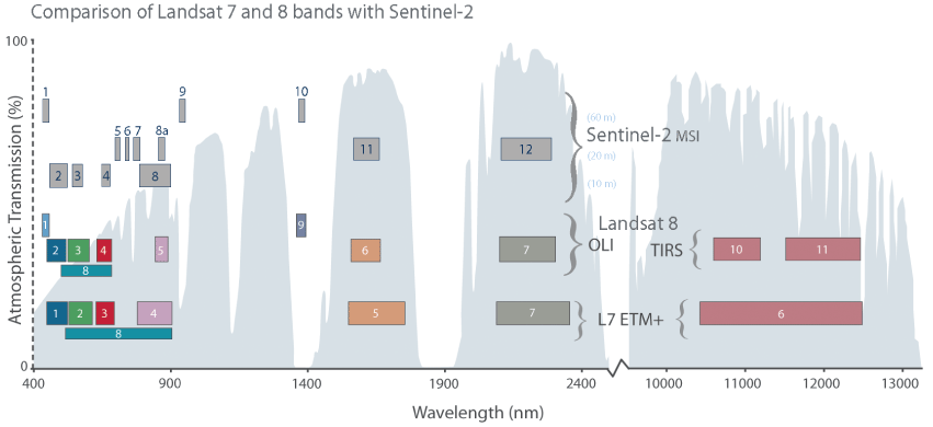
Graph showing comparison of Landsat 7 and Landsat 8 spectral bands with Sentinel-2 bands. %, percent; nm, nanometer. Source: https://landsat.gsfc.nasa.gov/wp-content/uploads/2015/06/Landsat.v.Sentinel-2.png (public domain).
Our searches of the Sentinel-2 archive for the eelgrass growing seasons of 2008 to 2023 found two dates when clear sky, low tide, and image acquisition all coincided; the data from these dates were suitable for spectral classification and eelgrass mapping throughout Izembek Lagoon (table 1).
Table 1.
All Sentinel-2 archived imagery suitable for mapping eelgrass at Izembek Lagoon, Alaska, during a 16-year period (2008–23).[The Level-1C archival image granule (tile) names are documented below the acquisition dates. Tide levels, in feet, relative to mean lower low water (MLLW) are shown at the time of image collection. The years of ground data (Ward, 2021) that contributed to map development and attribution are also shown. Image acquisition date given is year/month/day and hour/minute/second format. UTC, coordinated universal time;]
Image Pre-Processing
We downloaded the Sentinel Level-1C image tiles containing Izembek Lagoon for each of the two dates shown in table 1. The Level-1C product was delivered as terrain-corrected, top-of-atmosphere reflectances (the ratio between the incoming light and the light reflected after traveling through the atmosphere) in a georeferenced format (UTM Zone 3N), but otherwise, the Level-1C had the fewest alterations applied to the raw satellite image swath data compared to other Sentinel-2 image data formats. Each single tile from the two dates was cropped to the same 5,000-line by 6,000-sample image subset that fully encompassed Izembek Lagoon with 10-m pixel resolution and an upper left origin-pixel center-coordinate of ULX=6100005 and ULY=6155995. We resampled the 20-m bands to 10-m resolution using bilinear interpolation and stacked all bands into a 10-band composite image (table 2) for subsequent spectral analysis.
Table 2.
Structure and Sentinel-2 contents of a 10-band composite image used for spectral analysis.[Resolutions and center wavelengths of each band are shown. Band wavelengths are generalized into six categories: B, blue; G, green; R, red; NIR, near infrared; VNIR, very near infrared; and SWIR, shortwave infrared. Spectral bandwidths are illustrated in figure 1. m, meter; nm, nanometer]
We originally attempted to identify areas of change by clustering a combined 2-date 20-band image into 80 classes using the unsupervised algorithm ISODATA in the open-source software package MultiSpec© (version 9.2011, https://engineering.purdue.edu/~biehl/MultiSpec/). The class statistics were used with a Gaussian maximum likelihood classifier to assign each image pixel membership into one of the cluster classes. Evaluation of that classification, however, showed that the classes most often associated with change were primarily affected by changes in the physical environment such as alterations in mudflats, high-tide areas, and deep-water channels as opposed to changes in the biological environment. Consequently, we only used the combined 2-date classification to isolate the lagoon area by grouping all classes within the lagoon (except for obvious deep-water classes) and masking all remaining classes (that is, upland vegetation and deepwater). An elevation mask (elevation greater than 0 m) was additionally applied to exclude onshore water. The resulting mask included the intertidal areas of Izembek Lagoon (not areas of deep water), and some neighboring embayments (that is, Cold Bay and Kinzarof Lagoon) that were within the footprint of the Sentinel-2 image subsection. This mask was applied to both 10-band sub-sectioned images (that is, 2016 and 2020), and thereafter the two masked images were analyzed independently.
Image Spectral Analysis
Image analysis involved two parts. First, image pixels were split into cluster classes, and second, cluster classes were grouped into spectral classes. The splitting phase used ISODATA and the maximum likelihood classifier to derive and map 40 cluster classes from each 10-band masked image; hence, the cluster classes were specific to Izembek Lagoon proper. Forty clusters were prescribed—roughly twice the desired number of final classes.
The second phase grouped the cluster classes into a set of classes that were homogenous both spectrally and spatially. A series of iterations were performed to group the cluster classes into spectral classes. The overarching strategy was to maximize the number of spectral classes while reducing duplication of very similar classes. We applied five approaches to aid in the grouping process:
-
1. Calculation of a saturating transformed divergence metric, which is a measure of spectral separability between classes (Swain and King, 1973).
-
2. Calculation of an occurrence matrix that indicates which cluster classes are next to other classes spatially.
-
3. Use of a chaining algorithm that produces hierarchical cluster relations run on their separability (list item number 1), their occurrence (list item number 2), and on both combined (Aucoin and Stewart 1978).
-
4. Assessment of spectral biplots that graphed cluster means for two bands (that is, shortwave infrared [SWIR] × near infrared [NIR], Red versus NIR, etc.; for example, fig. 2).
-
5. Calculation of the number of ground data points in each cluster class to ensure the final spectral classes had a reasonable sample of field data for characterizing the associated eelgrass conditions.
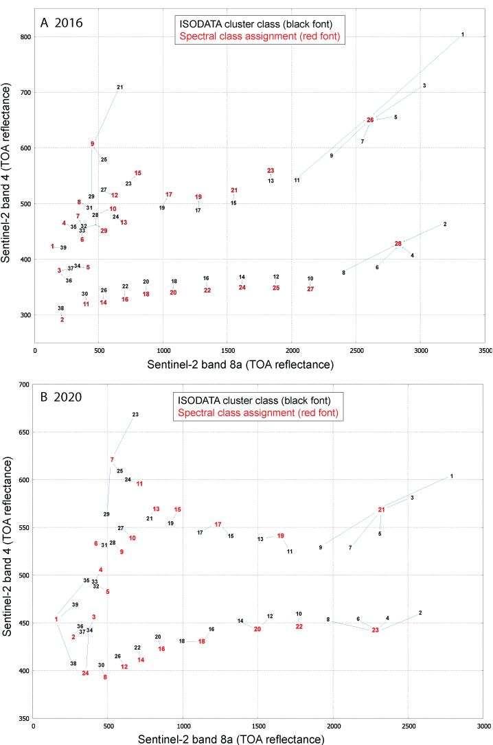
Spectral biplots showing cluster class means (denoted with black font) plotted on top of atmosphere (TOA) reflectance (unitless) of two spectral bands. Cluster class assignment in grouped (or split) spectral classes are denoted with red font (and positioned for legibility) for the (A) 2016 and (B) 2020 Sentinel-2 classifications of Izembek Lagoon, Alaska. Figure shows one of several strategies that guided the manual assignment of cluster classes into spectral classes, as summarized in table 3.
These approaches were collectively used to guide a visual and numerical interpretation of the cluster classes with the primary goal of grouping similar cluster classes into spectral classes. First, cluster classes clearly associated with pure water or mud flats (but not eelgrass classes) were identified and merged. This merging resulted in 36 and 35 cluster classes for the 2016 and 2020 images, respectively. Next, classes with a small or very small number of pixels were grouped into the spectrally and spatially closest (that is, “nearest”) class. Then, cluster classes that were spectrally and spatially very similar were grouped. Finally, classes with no or very few ground data were grouped with their most similar class. These steps served to produce spectrally and spatially homogeneous spectral classes by aggregating similar entities from the clustering step and ensuring that each class had field data. Figure 2 illustrates the assignment of cluster classes to spectral classes, mostly by grouping but with a few instances of splitting and masking. The biplots in figure 2 show an example of spectral relations between just two of Sentinel’s 10 spectral bands, meaning figure 2 shows an incomplete representation of the many spectral relations among clusters. Figure 2 is presented here to show how biplots can be a useful tool for guiding cluster groupings.
Following critical inspection of the spectral classes, two types of targeted adjustments to “problem classes” were applied to attain better spectral continuity. One adjustment type involved splitting a spectral class and the other involved masking pixels for supervised class reassignment. Specifically, in the 2020 image, one cluster appeared to contain at least two different classes based on its spectral and spatial characteristics. That cluster was then split into 10 classes using the 10-band spectral data and the ISODATA clustering algorithm. The 10 classes were assessed spectrally and spatially and grouped into 2 classes resulting in one class primarily in the southernmost part of the lagoon and seemed to be associated with deep water, and the other class more in the northern lagoon associated with shallower water. The 2020 clustering also required a supervised reassignment to the classification. A few isolated cloud shadows occurred on the mud flats in the northeastern lagoon, so a mask boundary was digitized by hand to encompass each area of cloud and cloud shadow, and then the cluster classes within the cloud mask (in this case, two classes) were changed to match the class of the surrounding mud flats. A similar supervised fix was applied to the 2016 map that involved remapping affected classes to a surrounding mudflat class. The last adjustment to both maps targeted areas on mud flats where large drifting accumulations of dislodged eelgrass and green seaweed often get deposited by tidal actions, and not surprisingly, get included in spectral classes associated with eelgrass. Using expert knowledge, field experience, and prior eelgrass maps, we hand digitized a custom mask of areas where large entanglements of drifting eelgrass and green seaweed often wash up onto mud flats, and then recoded eelgrass-associated spectral classes within that mask to a mud flat class. After all the groupings and custom adjustments described above were applied, there were 29 spectral classes for the 2016 Sentinel-2 image and 24 classes for the 2020 image. The sequence of steps and outcomes described above are summarized in table 3.
Table 3.
Sequence of steps applied to assign 40 cluster classes to spectrally and spatially similar spectral classes for each of the two Sentinel-2 image analyses (2016 and 2020) for Izembek Lagoon, Alaska.Field Data Preparation
Field data (Ward, 2021) that were collected onsite at spatially coincident sample plots were used to attribute each respective spectral class with information about the ground cover characteristics (that is, surface types like eelgrass, mud, water, etc.). Many years of field data have been collected at Izembek Lagoon (Ward, 2021) to monitor changes in eelgrass abundance and distribution (2007–11, 2015–19, 2022–23). Recognizing that changes are intrinsic to eelgrass communities (Ward and others, 2003; Bartenfelder and others, 2022; Munsch and others 2023), using ground data collected within 1 or 2 years of a satellite image collection date reduces the chances of the field data misrepresenting the actual ground conditions as recorded by the satellite image. For the 2016 Sentinel-2 image, we used field data collected in 2015 and 2016, and for the 2020 Sentinel-2 image, we used field data collected in 2018, 2019, and 2022 (table 1). We also added ground data from plots sampled in 2007 and 2008 where no eelgrass was observed, but only if those plots were not resampled in subsequent years because they had since remained in high intertidal areas beyond the growth range of eelgrass in the lagoon (Ward and others, 1997). Including the 2007 and 2008 ground data collected at persistent mudflats bolstered sample sizes used to characterize associated spectral classes.
Data from each field sampling plot were recorded in a four 0.25-square meter quadrat formats, arbitrarily positioned diagonally 5–10 m from the plot location in each of four compass-oriented quadrants (northwest, southwest, northeast, southeast; Ward, 2021). We diagonally positioned the UTM location of each sampled quadrat by adding and (or) subtracting 10 m to the plot’s UTM easting and northing, respective to the quadrant’s diagonal (northwest, southwest, northeast, southeast) compass direction. Including each of the four sampled quadrants at each plot, as well as the 2007–08 unvegetated plots, bolstered the number of samples used to characterize the spectral classes with information about the associated ground conditions.
Four variables recorded at each plot quadrat were specifically relevant for quantifying eelgrass conditions associated with each spectral class (table 4; percent cover, Braun-Blanquet cover category [Braun-Blanquet, 1972], presence, and abundance index). If a plot was sampled in more than 1 year, averages were calculated for each quadrant subplot.
Table 4.
Variables from the field data (Ward, 2021) that were used to quantify characteristics of each spectral class in terms of eelgrass fractional cover, presence, abundance, and biomass at Izembek Lagoon, Alaska.[m2, square meter; <, less than; =, equal; %, percent; mm, millimeter]
Spectral Class Attribution
The ground-plot quadrat data were spatially intersected with the spectral classes to calculate class-specific eelgrass cover statistics (mean, standard deviation, median, and interquartile range). Sometimes spectral classes were associated with notably different characterizations of ground cover. There are several explanations why a spectral class could be characterized by different ground data conditions, including (1) real changes in ground conditions between the dates of field sampling and satellite image collection; (2) accuracy of the field plot locations; (3) co-registration accuracies between the field plot locations and the georeferenced satellite image; (4) representativeness of the 0.25-square-meter quadrat relative to the 10 m×10 m Sentinel-2 grid cell; and (5) the choice of which Sentinel-2 grid cells to assign to each of the four sampled quadrants at each plot. For the last explanation, we assigned the sampled quadrants to the four grid cells on the diagonals of the grid cell that intersected the plot’s center location as opposed to the four cells in the cardinal directions.
Recognizing the high likelihood that some misrepresentative ground data gets included in calculations of class-specific eelgrass cover statistics, before those statistics were finalized, we first excluded the more egregious outliers of this ground data for each variable (table 4) within each spectral class. Outliers were defined as any data records with values outside (greater than or less than) the 1.5×interquartile range. After the outliers were excluded, we recalculated and graphed the class-specific statistics for each eelgrass variable as violin plots (app. 1, figs. 1.1–1.4) and tabulated the corresponding means, medians, and variances (app. 1, tables 1.1–1.8). The modeled eelgrass biomass estimates and 95-percent credible intervals (Patil, 2024) were calculated for each field plot location (not quad) so sample size intersecting each spectral class was four times smaller than the other field data metrics (app. 1, fig. 1.5). Consequently, we derived biomass maps from median values only (app. 1, tables 1.9, 1.10) because the mean values were sometimes unrealistically skewed.
Eelgrass Mapping
Our eelgrass-mapping strategy at Izembek Lagoon began with unsupervised derivation of statistical cluster classes that we subsequently grouped into spectral classes and then attributed with environmental data from field studies. In other words, the spectral classes established a gradient (or scale) of environmental conditions, and the ground data served to calibrate that scale. The underlying assumption of this strategy is that surface areas with similar cover characteristics will also possess similar spectral characteristics, which in turn will be grouped (clustered) into like spectral classes and thus provide useful information about the spatial distributions of surface-cover types throughout the study area.
Eelgrass maps were produced by attributing each spectral class with an eelgrass statistic of choice derived from field observations (after outliers had been excluded). Maps were generated for each of the five eelgrass variables in table 4. For example, a map of median eelgrass percentage of cover was produced by deriving the median for each spectral class from the ground plot data that spatially intersected the respective classes (fig. 3A, 3B), and similarly, a map of median eelgrass biomass was produced (fig. 3C, 3D).
All maps of spectral classes, eelgrass attributes, and derivative maps of eelgrass metrics in geoTIFF and CSV format are available in Douglas and others (2024).
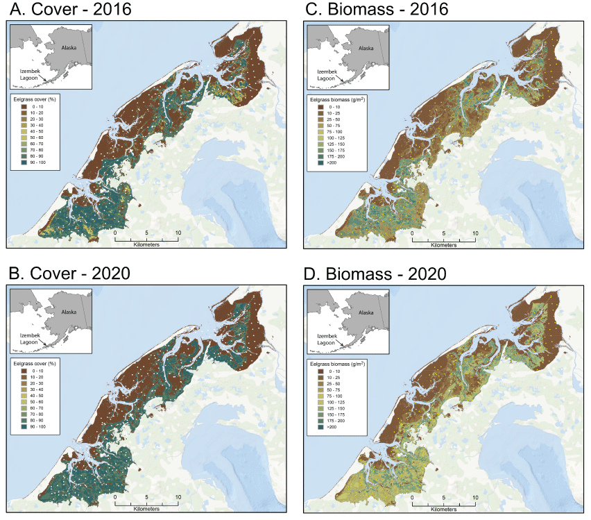
Maps showing (A, B) median eelgrass cover and (C, D) eelgrass biomass at Izembek Lagoon, Alaska, derived from Sentinel-2 satellite images collected during low tide on July 1, 2016 (A, C), and August 14, 2020 (B, D). Twenty-nine spectral classes were generated from the 2016 Sentinel-2 image, and 24 spectral classes were generated from the 2020 Sentinel-2 image, and then field data (Ward, 2021; Patil, 2024) collected throughout the lagoon were used to characterize each spectral class with respect to the field data collected there. In these maps, each spectral class has been color shaded based on the median eelgrass as directly observed (cover) or model estimated (biomass) at spatially coincident field plots (dots). %, percent; g/m2, grams per square meter. Digital maps and eelgrass data are available in Douglas and others (2024).
Earlier Landsat-Derived Eelgrass Maps
Two prior eelgrass maps of Izembek Lagoon were produced from Landsat satellite imagery (Ward and others, 1997; Hogrefe and others, 2014). Both Landsat maps used ISODATA methods initially, like what was done for the Sentinel imagery described above, but thereafter, the methods of eelgrass mapping differed and are described here for comparison.
The first eelgrass map of Izembek Lagoon (Ward and others, 1997) was produced from a July 28, 1978, Landsat-3 multispectral scanner satellite image consisting of 4 spectral bands with 50-m pixel resolution collected during a late morning (11:14 a.m. local Alaska time) tide at −0.3 ft. ISODATA was applied to partition the image data encompassing the lagoon into 33 cluster classes, and then each pixel in the image was assigned to a cluster class using a maximum likelihood estimation (MLE) classifier. Each cluster class was subsequently labelled as water, eelgrass, unvegetated, or upland based on personal knowledge of the area, a review of black and white aerial photographs taken in June 1976, and ground data collected in 1986. Two final steps involved changing pixels classified as eelgrass in upland areas to the upland class, and similarly, changing small areas of eelgrass (≤2 pixels) surrounded by unvegetated areas to unvegetated.
The second eelgrass map of Izembek Lagoon (Hogrefe and others, 2014) was produced from a combination of two Landsat images: one collected on August 2, 2002, by Landsat-7-ETM+ at a tide level of +0.03 feet and the other on July 20, 2006, by Landsat-5-TM at a −0.27 tide. Two images were used (instead of one) to overcome some isolated cloud contaminations that did not overlap spatially. Each image was classified independently by first masking dry land and clouds and then using ISODATA to derive 35 cluster classes. Clusters were assigned to one of eight substrate classes to create eight training regions: four for eelgrass and two each for bare ground and water (or left unassigned if uncertain). Clusters spatially coinciding with areas of assumed eelgrass based on false-color enhancements of Landsat bands 4, 5, and 1 were manually assigned to one of four eelgrass classes based on the relative strengths of band-4 (near infrared) and band-3 (red) radiances: (1) high NIR, (2) moderate NIR, (3) low NIR, and (4) minimal NIR. Similarly, classes representing bare ground or water were determined by visual interpretation and partitioned into two respective subclasses, also based on spectral radiance profiles: dry or wet bare ground and shallow/turbid or deep/clear water. Then, all assigned clusters were merged to create discrete training clusters for a MLE classification that assigned every pixel to one of the eight substrate classes. To overcome small amounts of cloud contamination, the two maps were mosaiced with the 2002 map covering the southern one-third of the lagoon and the 2006 map covering the northern two-thirds. A final manual step changed small, isolated patches of eelgrass on bare ground to a ninth map class, seaweed. We refer to this map hereinafter as the 2006 Landsat map.
The initial unsupervised derivation of roughly 35–40 cluster classes by use of ISODATA was common to the Landsat and Sentinel satellite mapping approaches used in this study. Thereafter, however, both the Landsat approaches used a greater degree of subjective supervision than did the Sentinel approach. For the 1978 Landsat-3 map, the initial suite of 33 cluster classes were each manually assigned to one of four map classes based on expert interpretations of aerial photographs, spatial context, and field data. For the 2006 Landsat-7 map, the initial 35 cluster classes were manually assigned to one of eight training classes based on spatial context as well as spectral relations among the red and infrared imagery bands. Clusters assigned to each of the eight training classes were then merged, and those eight merged clusters were used with MLE to produce a map specifically of those eight defined substrate classes.
The Sentinel method began by developing a set of cluster classes with ISODATA, and then some were split or merged based on spectral relations, spatial juxtapositions, and sample sizes. Few presumptions or supervised attributions about surface cover were imposed on cluster assignments. The set of clusters was used instead to produce a map of spectral classes, and then each spectral class was attributed with surface-cover information by quantifying ground data collected within each class’s spatial footprint. In other words, our Sentinel mapping method transformed a static map of derived cluster classes into a map of surface cover by attributing each class with a summary of ground data about a metric of interest (for example, fig. 3). Having an adequate representation of ground conditions to robustly characterize the spectral classes, this strategy provides objectivity and utility owing to the breadth of map themes that can be derived for a variety of mapping goals.
Results
Analyses of legacy and contemporary eelgrass maps derived from satellite imagery can expose changes in eelgrass distribution at Izembek Lagoon over time. Key assumptions, findings, and caveats of our change detection analyses are described below.
Eelgrass Change Detection
Eelgrass changes at Izembek Lagoon can be estimated and quantified by subtracting two eelgrass maps depicting conditions in different years. The two maps must represent the same eelgrass metric, so the areas where the two maps disagree should presumably show areas where eelgrass had increased or decreased. However, map-detected changes are susceptible to false positives caused by factors other than real on-the-ground changes. Two influential factors stem from differences in (1) the precise tide level at the time when the images were collected; and (2) the seasonal phenology of eelgrass growth on the date when images were collected. Areas of eelgrass growth that are partially submerged at low tide and (or) possess only sparse eelgrass cover will be more challenging to robustly detect in imagery that is collected at a time when the tide is only slightly negative. Similarly, analyzing imagery of eelgrass that is many weeks from the time of peak growth will tend to diminish eelgrass detectability. These two factors (tide level and phenology) should be considered when interpreting map-derived changes, especially changes involving areas associated with marginal (sparse) eelgrass cover or deeper water.
The 2006 Landsat map of eelgrass at Izembek Lagoon delineated four spectral classes associated with areas of eelgrass with varying levels of near-infrared reflectance (Hogrefe and others, 2014). For the purposes of detecting eelgrass changes between the 2006 Landsat map of eelgrass and either the 2016 or 2020 Sentinel-2 eelgrass maps, we considered all four Landsat eelgrass classes to be representative of eelgrass presence. For the two Sentinel-2 eelgrass maps, we considered all spectral classes with a median Braun-Blanquet cover value greater than 1.0 (app. 1, fig. 1.6) to be comparable to the four combined Landsat classes of eelgrass. With those definitions, eelgrass presence/absence maps were generated for each of the three mapping years (2006, 2016, and 2020). Each pair of these derivative two-class (present/absent) eelgrass maps was then differenced to spatially depict where eelgrass was gained, lost, or unchanged from the earlier map year to the later map year. For illustration, we show results for the three difference maps (fig. 4), as well as the net areal extent (in square kilometers [km2]) of those mapped changes in eelgrass presence (table 5). Roughly 40 km2 of area that supported eelgrass in 2006 was lost by 2020, whereas about 15 km2 of eelgrass was gained, resulting in a net loss of about 25 km2 (table 5). From 2006 to 2020, most areas where the presence of eelgrass was lost were in the central part of Izembek Lagoon (fig. 4).
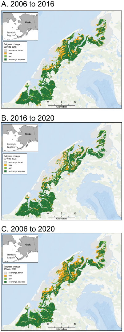
Map showing areas where the presence of eelgrass was gained, lost, or unchanged in Izembek Lagoon, Alaska, from (A) 2006 to 2016, (B) 2016 to 2020, and (C) 2006 to 2020.
Table 5.
Net spatial extent of eelgrass presence gained, lost, or unchanged in Izembek Lagoon, Alaska, from 2006 to 2016, 2016 to 2020, and 2006 to 2020.[Area calculations do not include the Lagoon’s deep-water channels. km2, square kilometer]
Spatial changes in estimated modeled biomass from the first Sentinel-2 imagery (July 1, 2016) to the second imagery e (August 14, 2020) are shown in figure 5 and were calculated by subtracting the two biomass maps from figure 3. Although eelgrass biomass changed substantially over the course of a growing season (Ward and others, 2022), the biomass model adjusted for day of year and tide level (Ward and Amundson, 2019), so the two maps were better standardized with respect to phenology and thus better suited for revealing between-year changes in community density or vigor as might be affected by storm events, water temperature fluctuations, or winter ice scouring.
We multiplied the biomass estimate for each spectral class in both Sentinel-2 maps (as mapped in fig. 3) by the respective class’s aerial extent, and then summed across all classes to derive an estimate of the total eelgrass biomass throughout Izembek Lagoon on each respective image date (table 6). The same methods used to attribute spectral classes by intersecting the plot estimates of biomass and assigning the spectral classes with median values after outliers were removed were similarly applied using each ground plot’s upper (97.5-percent) and lower (2.5-percent) bounds of the 95-percent biomass credible interval (table 6). The modest net increase in lagoon-wide biomass from 2016 to 2020 (table 6) was inconclusive considering the broad 95-percent credible intervals of the annual point estimates.
Table 6.
Estimated total eelgrass biomass in Izembek Lagoon, Alaska, on July 1, 2016, and August 14, 2020.[All table numbers in metric tons. Lower and upper 95-percent credible interval (CI) are the upper and lower bounds of 95-percent Bayesian credible intervals. , percent; CI, credible interval; +, plus]
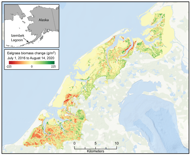
Map showing estimated change in eelgrass biomass at Izembek Lagoon, Alaska, from July 1, 2016, to August 14, 2020.
Conclusions
Findings of this study highlight the utility of using satellite remote sensing technologies, such as Sentinel-2, together with in situ ground observations for monitoring eelgrass over large geographic areas like Izembek Lagoon, Alaska. The approach produced updated, publicly accessible, high-resolution digital maps of eelgrass distribution, cover, and biomass of Izembek Lagoon. The mapping results indicated a net loss of eelgrass extent from 2006 to 2020 concentrated in the central lagoon, and biomass reductions from 2016 to 2020 that were concentrated in the southern lagoon but offset by biomass gains in the central and northern lagoon.
References Cited
Aucoin, P.J., and Stewart, J., 1978, Earth Observations Division version of the Laboratory for Applications of Remote Sensing system (EOD-LARSYS) user guide for the IBM 370/148 Volume 1-System overview: Earth Observations Division Space and Life Sciences Directorate JSC–13821, prepared by Lockheed Electronics Company, Inc., Systems and Services Division under contract, Houston, Tex., 227 p. [Also available at https://ntrs.nasa.gov/api/citations/19800018225/downloads/19800018225.pdf.]
Bartenfelder, A., Kenworthy, W.J., Puckett, B., Deaton, C., and Jarvis, J.C., 2022, The abundance and persistence of temperate and tropical seagrasses at their edge-of-range in the Western Atlantic Ocean: Frontiers in Marine Science, v. 9, p. 917237, accessed August 13, 2024, at https://doi.org/10.3389/fmars.2022.917237.
Douglas, D.C., Fleming, M.D., Patil, V., and Ward, D.H., 2024, Eelgrass (Zostera marina) maps from 2016 and 2020, at Izembek Lagoon, Alaska: U.S. Geological Survey data release, accessed August 13, 2024, at https://doi.org/10.5066/P1HLTAHD.
Drusch, M., Del Bello, U., Carlier, S., Colin, O., Fernandez, V., Gascon, F., Hoersch, B., Isola, C., Laberinti, P., Martimort, P., Meygret, A,Spoto, F., Sy, O., Marchese, F., and Bargellini, P., 2012, Sentinel-2—ESA’s optical high-resolution mission for GMES operational services: Remote Sensing of Environment, v. 120, p. 25–36, accessed August 13, 2024, at, https://doi.org/10.1016/j.rse.2011.11.026.
Hogrefe, K.R., Ward, D.H., Donnelly, T.F., and Dau, N., 2014, Establishing a baseline for regional scale monitoring of eelgrass (Zostera marina) habitat on the lower Alaska Peninsula: Remote Sensing, v. 6, no. 12, p. 12447–12477, accessed August 13, 2024, at https://doi.org/10.3390/rs61212447.
Li, J., and Roy, D.P., 2017, A global analysis of Sentinel-2A, Sentinel-2B and Landsat-8 data revisit intervals and implications for terrestrial monitoring: Remote Sensing, v. 9, no. 9, 902, accessed August 13, 2024, at https://doi.org/10.3390/rs9090902.
Loveland, T.R., and Irons, J.R., 2016, Landsat 8—The plans, the reality, and the legacy: Remote Sensing of Environment, v. 185, p. 1–6, accessed August 13, 2024, at https://doi.org/10.1016/j.rse.2016.07.033.
Munsch, S.H., Beaty, F.L., Beheshti, K.M., Chesney, W.B.,Endris, C.A., Gerwing, T.G., Hessing-Lewis, M., Kiffney, P.M., O’Leary, J.K., Reshitnyk, L., Sanderson, B.L., and Walter, R.K., 2023, Northeast Pacific eelgrass dynamics—Interannual expansion distances and meadow area variation over time: Marine Ecology Progress Series, v. 705, p. 61–75, accessed August 13, 2024, at https://doi.org/10.3354/meps14248.
Neckles, H.A., Kopp, B.S., Peterson, B.J., and Pooler, P.S., 2012, Integrating scales of seagrass monitoring to meet conservation needs: Estuaries and Coasts, v. 35, p. 23–46, accessed August 13, 2024, at https://doi.org/10.1007/s12237-011-9410-x.
Overland, J.E., Siddon, E., Sheffield, G., Ballinger, T.J., and Szuwalski, C., 2024, Transformative ecological and human impacts from diminished sea ice in the northern Bering Sea: Weather, Climate, and Society, v. 16, no. 2, p. 303–313, accessed August 13, 2024, at https://doi.org/10.1175/WCAS-D-23-0029.1.
Patil, V.P., 2024, Eelgrass biomass model (ver. 1.0.1, May 2024): U.S. Geological Survey software release, accessed August 13, 2024, at https://doi.org/10.5066/P13EG9KS.
Phiri, D., Simwanda, M., Salekin, S., Nyirenda, V.R., Murayama, Y., and Ranagalage, M., 2020, Sentinel-2 data for land cover/use mapping—A review: Remote Sensing, v. 12, no. 14, 2291, accessed August 13, 2024, at https://doi.org/10.3390/rs12142291.
Ramsar, 2023, The list of wetlands of international importance: The Secretariat of the Convention on Wetlands, accessed August 13, 2024, at https://www.ramsar.org/sites/default/files/documents/library/sitelist.pdf.
Sherman, K., and DeBruyckere, L.A., 2018, Eelgrass habitats on the U.S. West Coast—State of the knowledge of eelgrass ecosystem services and eelgrass extent: Prepared by the Pacific Marine and Estuarine Fish Habitat Partnership for The Nature Conservancy, 67 p., accessed August 13, 2024, at https://www.pacificfishhabitat.org/wp-content/uploads/2017/09/EelGrass_Report_Final_ForPrint_web.pdf.
Swain, P.H., and King, R.C., 1973, Two effective feature selection criteria for multispectral remote sensing: LARS Technical Reports, Paper 39, accessed August 13, 2024, at https://docs.lib.purdue.edu/larstech/39.
Ward, D.H., Markon, C.J., and Douglas, D.C., 1997, Distribution and stability of eelgrass beds at Izembek Lagoon, Alaska: Aquatic Botany, v. 58, p. 229–240, accessed August 13, 2024, at https://doi.org/10.1016/S0304-3770(97)00037-5.
Ward, D.H., Morton, A., Tibbitts, T.L., Douglas, D.C., and Carrera-Gonzalez, E., 2003, Long-term change in eelgrass distribution at Bahia San Quintin, Baja California, Mexico, using satellite imagery: Estuaries, v. 26, p. 1529–1539, accessed August 13, 2024, at https://doi.org/10.1007/BF02803661.
Ward, D.H., 2021, Point sampling data for eelgrass (Zostera marina) and seaweed distribution and abundance in bays adjacent to the Izembek National Wildlife Refuge, Alaska (ver. 4.0, June 2024): U.S. Geological Survey data release, accessed August 13, 2024, at https://doi.org/10.5066/P9ZUDIOH.
Ward, D.H., and Amundson, C.L., 2019, Monitoring annual trends in abundance of eelgrass (Zostera marina) at Izembek National Wildlife Refuge, Alaska, 2018: U.S. Geological Survey Open-File Report 2019-1042, 8 p., accessed August 13, 2024, at https://doi.org/10.3133/ofr20191042.
Ward, D.H., Hogrefe, K.R., Donnelly, T.F., Fairchild, L.L., Sowl, K.M., and Lindstrom, S.C., 2022, Abundance and distribution of eelgrass (Zostera marina) and seaweeds at Izembek National Wildlife Refuge, Alaska, 2007–10: U.S. Geological Survey Open-File Report 2020–1035, 30 p., accessed August 13, 2024, at https://doi.org/10.3133/ofr20201035.
Wood, K.R., Bond, N.A., Danielson, S.L., Overland, J.E., Salo,S.A., Stabeno, P.J., and Whitefield, J., 2015, A decade of environmental change in the Pacific Arctic region: Progress in Oceanography, v. 136, p. 12–31, accessed August 13, 2024, at https://doi.org/10.1016/j.pocean.2015.05.005.
Appendix 1. Ground Data Statistics for Each Spectral Class
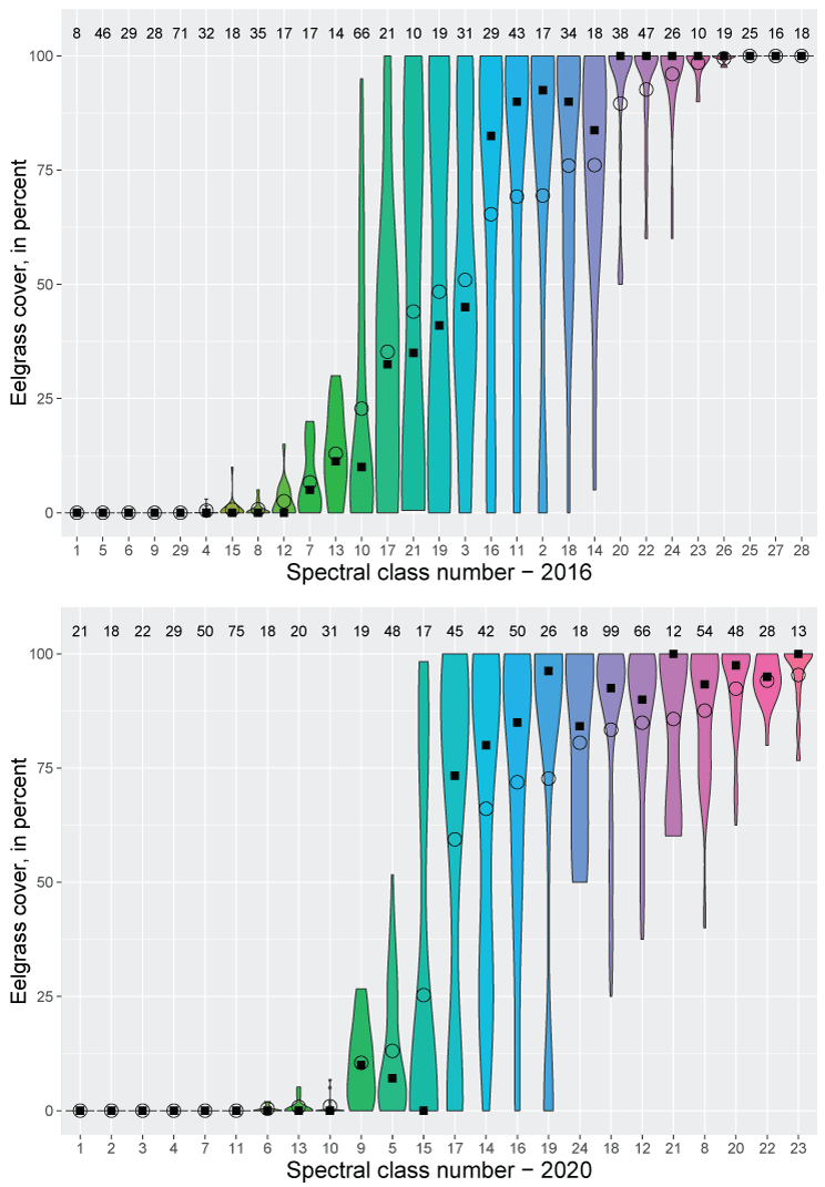
Violin plots showing percentage of eelgrass cover within each of the 29 spectral classes derived from the 2016 Sentinel-2 image (top) and the 24 spectral classes derived from the 2020 Sentinel-2 image (bottom). Class means are shown with an open circle, and medians are shown with a solid square. Spectral classes are sorted by ascending mean percentage of eelgrass cover. Violin shape depicts the frequency distribution of observations, scaled to constant width across classes. Ground-data sample sizes are shown across the top.
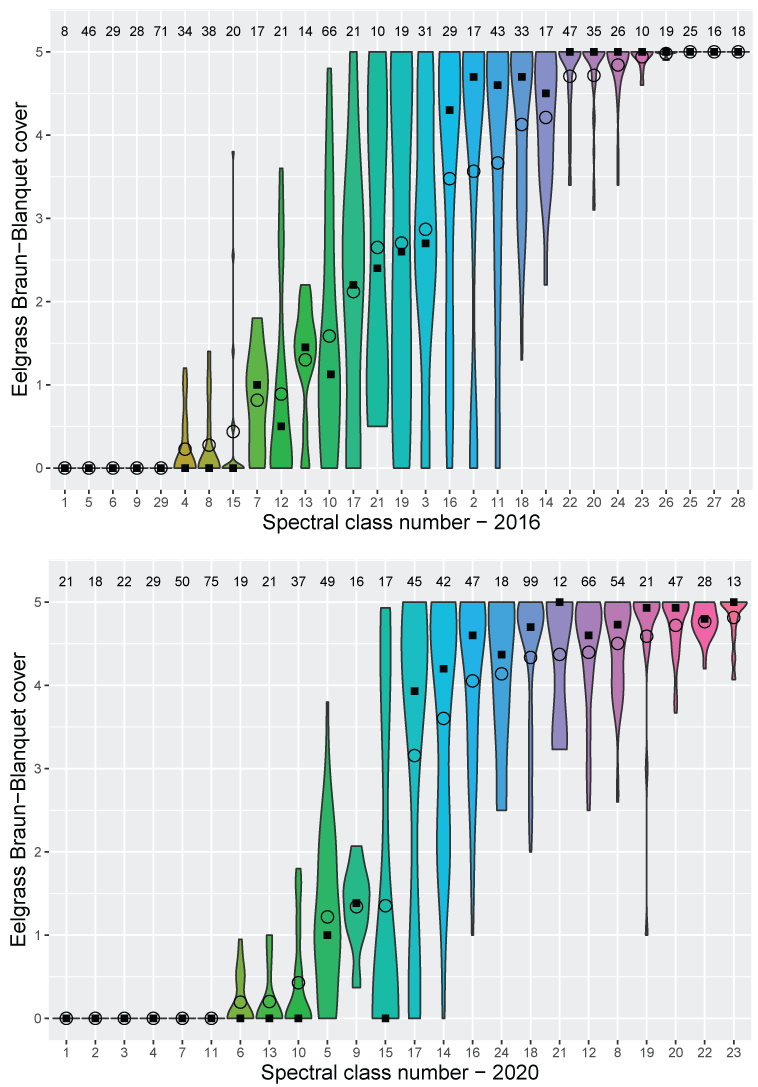
Violin plots showing eelgrass Braun-Blanquet cover within each of the 29 spectral classes from the 2016 Sentinel-2 image (top) and the 24 spectral classes derived from the 2020 Sentinel-2 image (bottom). Class means are shown with an open circle, and medians with a solid square. Spectral classes are sorted by ascending mean Braun-Blanquet eelgrass cover. Violin shape depicts the frequency distribution of observations, scaled to constant width across classes. Ground-data sample sizes are shown across the top.
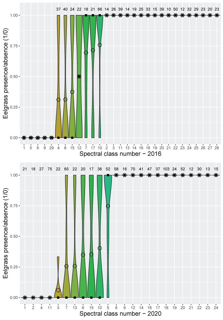
Violin plots showing eelgrass presence (1) or absence (0) within each of the 29 spectral classes derived from the 2016 Sentinel-2 image (top) and the 24 spectral classes derived from the 2020 Sentinel-2 image (bottom). Class means are shown with an open circle, and medians are shown with a solid square. Spectral classes are sorted by ascending mean. Sample sizes are shown across the top. Violin shape depicts the frequency distribution of observations, scaled to constant width across classes. Ground-data sample sizes are shown across the top.
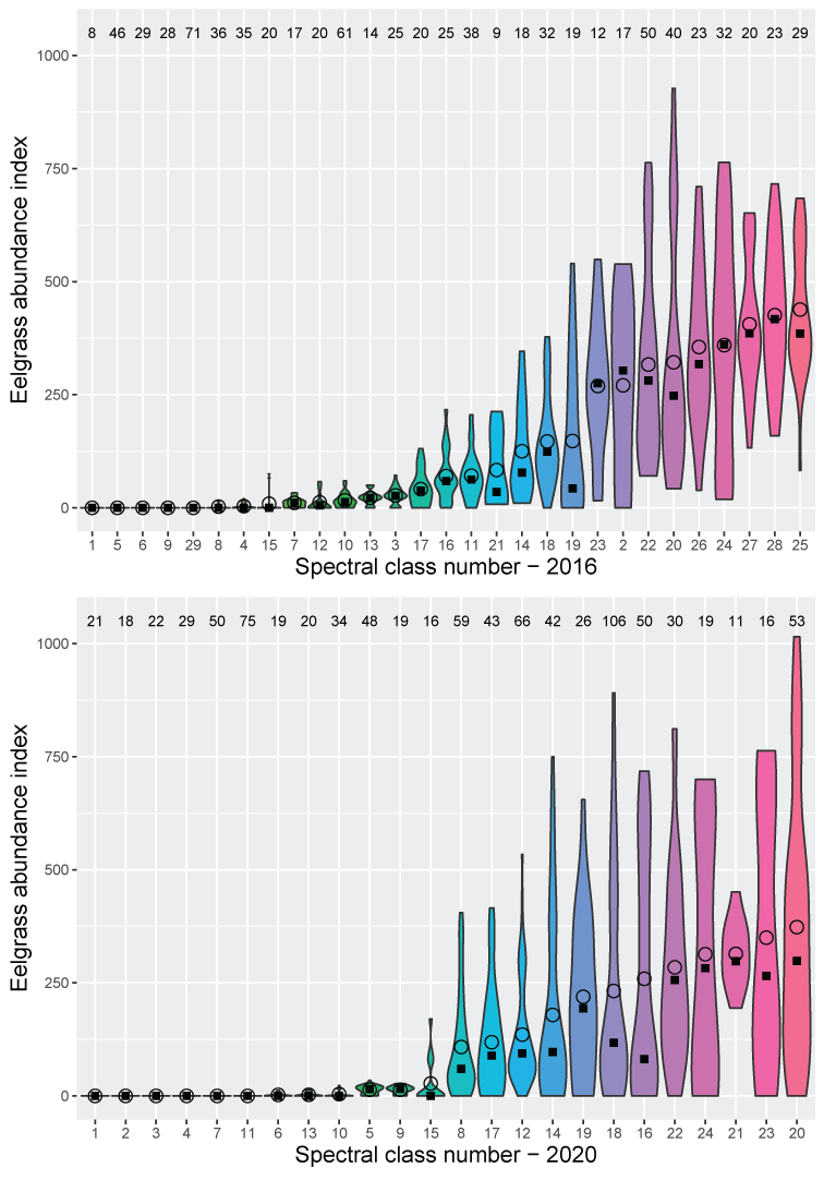
Violin plots showing eelgrass abundance index within each of the 29 spectral classes derived from the 2016 Sentinel-2 image (top) and the 24 spectral classes derived from the 2020 Sentinel-2 image (bottom). Class means are shown with an open circle, and medians are shown with a solid square. Spectral classes are sorted by ascending mean sample sizes are shown across the top. Violin shape depicts the frequency distribution of observations, scaled to a constant width across classes. Ground-data sample sizes are shown across the top.
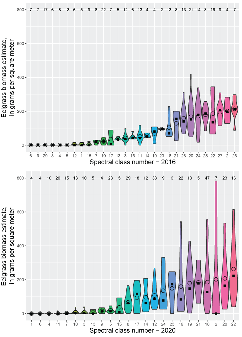
Violin plots showing eelgrass biomass estimates within each of the 29 spectral classes derived from the 2016 Sentinel-2 image (top) and the 24 spectral classes derived from the 2020 Sentinel-2 image (bottom). Class means are shown with an open circle, and medians are shown with a solid square. Spectral classes are sorted by ascending mean sample sizes and are shown across the top. Violin shape depicts the frequency distribution of observations, scaled to a constant width across classes. Ground-data sample sizes are shown across the top.
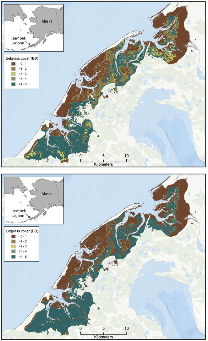
Maps showing median eelgrass Braun-Blanquet cover at Izembek Lagoon, Alaska, derived from a Sentinel-2 satellite image collected during low tide on July 1, 2016 (top), and on August 14, 2020 (bottom). Twenty-nine/24 spectral classes were generated from the 2016/2020 Sentinel-2 multispectral images within the lagoon. In these maps, each spectral class has been color-shaded based on the median Braun-Blanquette (BB) cover category that was recorded at field plots located within the respective classes. >, greater than.
Table 1.1.
Eelgrass percentage of cover statistics for each 2020 Sentinel-2 spectral class.[Spectral classes are sorted by mean percentage of cover. N, number; Std. dev., standard deviation; IQR, interquartile range]
Table 1.2.
Braun-Blanquet (BB) cover category statistics for eelgrass for each 2020 Sentinel-2 spectral class.[Spectral classes sorted by mean BB cover. N, number; Std. dev., standard deviation; IQR, interquartile range]
Table 1.3.
Eelgrass presence (binary) statistics for each 2020 Sentinel-2 spectral class.[Spectral classes sorted by mean presence. N, number; Std. dev., standard deviation; IQR, interquartile range]
Table 1.4.
Eelgrass abundance index statistics for each 2020 Sentinel-2 spectral class.[Spectral classes sorted by mean abundance indexes. N, number; Std. dev., standard deviation; IQR, interquartile range]
Table 1.5.
Eelgrass percentage of cover statistics for each 2016 Sentinel-2 spectral class.[Spectral classes sorted by mean percentage of cover. N, number; Std. dev., standard deviation; IQR, interquartile range]
Table 1.6.
Braun-Blanquet cover category statistics for eelgrass for each Sentinel-2 spectral class.[Spectral classes sorted by mean percentage of cover category. N, number; Std. dev., standard deviation; IQR, interquartile range]
Table 1.7.
Eelgrass presence (binary) statistics for each 2016 Sentinel-2 spectral class.[Spectral class sorted by mean presence. N, number; Std. dev., standard deviation; IQR, interquartile range]
Table 1.8.
Eelgrass abundance index statistics for each 2016 Sentinel-2 spectral class.[Spectral class sorted by mean abundance index. N, number; Std. dev., standard deviation; IQR, interquartile range]
Table 1.9.
Median eelgrass biomass estimates for each 2020 Sentinel-2 spectral class.[Spectral class sorted by biomass. N, number; g/m2, grams per square meter; %, percent; CI, credible interval]
Table 1.10.
Median eelgrass biomass estimates for each 2016 Sentinel-2 spectral class.[Spectral class sorted by biomass. N, number; g/m2, grams per square meter; %, percent; CI, credible interval]
Conversion Factors
Temperature in degrees Celsius (°C) may be converted to degrees Fahrenheit (°F) as follows:
°F = (1.8 × °C) + 32.
Temperature in degrees Fahrenheit (°F) may be converted to degrees Celsius (°C) as follows:
°C = (°F – 32) / 1.8.
For additional information, contact:
Director, U.S. Geological Survey Alaska Science Center
4210 University Drive
Anchorage, AK 99508
For additional information, visit: https://www.usgs.gov/centers/alaska-science-center
Disclaimers
Any use of trade, firm, or product names is for descriptive purposes only and does not imply endorsement by the U.S. Government.
Although this information product, for the most part, is in the public domain, it also may contain copyrighted materials as noted in the text. Permission to reproduce copyrighted items must be secured from the copyright owner.
Suggested Citation
Douglas, D.C., Fleming, M.D., Patil, V.P., and Ward, D.H., 2025, Mapping eelgrass (Zostera marina) cover and biomass at Izembek Lagoon, Alaska, using in-situ field data and Sentinel-2 satellite imagery: U.S. Geological Survey Open-File Report 2025–1007, 30 p., https://doi.org/10.3133/ofr20251007. [Supersedes preprint https://doi.org/10.1101/2024.08.07.607047.]
ISSN: 2331-1258 (online)
Study Area
| Publication type | Report |
|---|---|
| Publication Subtype | USGS Numbered Series |
| Title | Mapping eelgrass (Zostera marina) cover and biomass at Izembek Lagoon, Alaska, using in-situ field data and Sentinel-2 satellite imagery |
| Series title | Open-File Report |
| Series number | 2025-1007 |
| DOI | 10.3133/ofr20251007 |
| Publication Date | May 16, 2025 |
| Year Published | 2025 |
| Language | English |
| Publisher | U.S. Geological Survey |
| Publisher location | Reston, VA |
| Contributing office(s) | Alaska Science Center Ecosystems |
| Description | Report: vii, 30 p.; Data Release |
| Country | United States |
| State | Alaska |
| Other Geospatial | Izembek Lagoon |
| Online Only (Y/N) | Y |