

Suspended Sediment and Bedload Transport Along the Main and South Branches, Wild Rice River, Northwestern Minnesota, 1979 through 2023
Links
- Document: Report (4.2 MB pdf) , HTML , XML
- Dataset: USGS National Water Information System database - USGS water data for the Nation
- NGMDB Index Page: National Geologic Map Database Index Page (html)
- Download citation as: RIS | Dublin Core
Acknowledgments
This report presents a compilation of information, resources, and expertise supplied by many individuals. The authors would like to thank the Wild Rice Watershed District and Jerry Bents of Houston Engineering for their assistance with this study. Christopher Ellison and Scott Anderson of the U.S. Geological Survey are acknowledged for their technical reviews of the report.
Abstract
The geologic history and anthropogenic modifications of Minnesota’s Wild Rice River have caused major morphological adjustments, which induce erosion and excess fluvial sediment transport. The excess sediment deposits in the lower Wild Rice River, exacerbating flooding. To help mitigate these problems, the Wild Rice Watershed District has future plans to implement a river restoration on the lower Wild Rice River. The Wild Rice Watershed District collaborated with the U.S. Geological Survey to measure and analyze sediment transport along the Wild Rice River’s Main and South Branches to assess any potential changes in sediment transport among sites and time periods. Time differencing results indicated that all suspended-sediment constituents showed a significant difference between the two sampling periods at one South Branch site but not at the Main Branch site. Piecewise regression analysis better matched the suspended-sediment constituents transport process at most sites by differentiating no relation between suspended-sediment constituents at lower streamflows and a positive relation at higher streamflows at most Wild Rice River sites. Five of the sites showed elevated sediment transport with increasing streamflow. In contrast, the site farthest downstream showed a negative relation with increasing streamflow, indicating that that the lower Wild Rice River is supply limited and deposition is likely occurring upstream and (or) near the site. Overall, the uncertainty in results indicates the complexity of sediment transport in a river when using streamflow as the sole explanatory variable and suggests a need for multisite, multiyear, and multifaceted data.
Introduction
The Wild Rice River (fig. 1) in northwestern Minnesota has a history of and continues to undergo major morphological adjustments and experience flooding, which is exacerbated by excess sediment transport and deposition of fluvial sediment. These outcomes are influenced by the river’s geologic history, nearby land use, and anthropogenic modifications to the channel, such as drainage ditches and flood control structures. Understanding fluvial sediment transport processes is essential with respect to channel morphology, reservoir and channel storage, aquatic habitat, flooding, and river restorations. In Minnesota, sediment and siltation are two of the leading causes of impairments in rivers and streams (Minnesota Pollution Control Agency, 2024). The Wild Rice Watershed District (WRWD) has future plans of implementing a river restoration of the Wild Rice River by setting flood levees back, which is intended to widen the stream corridor, and reconstructing meanders in the channel by increasing the floodplain area, which could help mitigate excess flooding, erosion, deposition of sediment, and sediment related water quality concerns.
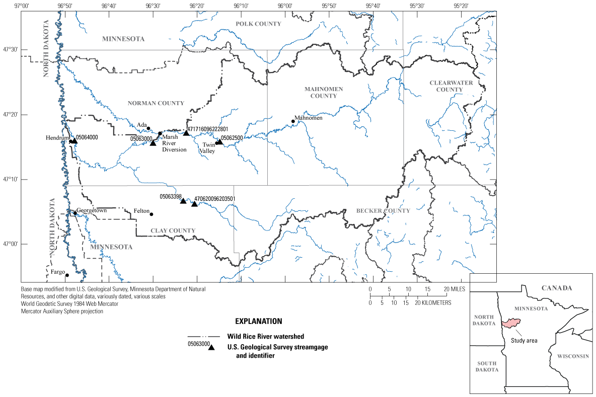
Study area map of Wild Rice River Basin, rivers and streams, sampling sites, and towns.
Fluvial sediment data that have been collected along the Main and South Branch Wild Rice Rivers and could be used to help inform future river restoration designs. Fluvial sediment data collected for this report include both suspended-sediment constituents and bedload. These data are needed to help understand the timing, frequency, and magnitude of total sediment transport, and its relation with streamflow.
Sediment rating curves (SRCs) are regression equations for suspended-sediment constituents (all three constituents are defined in the “Methods of Data Collection and Analysis” section) and bedload and can be used as a predictive tool to estimate sediment transport. Although numerous computer-based sediment transport models are available, they often do not match sampled data within acceptable limits (Lopes and others, 2001; Barry and others, 2008). It is common for streamflow and sampled sediment data to be uncorrelated, which can be caused by a myriad of sediment supply and transport processes and is generally referred to as hysteresis (Gellis, 2013). There were SRCs developed at select Wild Rice River sites as part of previous studies, and the SRCs were site-specific log-linear regression equations for the entire streamflow regime (Ellison and others, 2014, 2016). In addition, Ellison and others (2014) evaluated turbidity as a surrogate to estimate suspended-sediment concentration (SSC). Using turbidity was more accurate than just using streamflow as an explanatory variable, resulting in higher coefficients of determinations (R2).
Purpose and Scope
The purpose of this report is to describe the measurement and analysis of suspended-sediment constituents and bedload along the Wild Rice’s Main and South Branches and the assessment of potential changes in sediment transport among sites in different geologic, erosional, and depositional areas and with different sampling periods of record. Specifically, the report describes relations among suspended-sediment constituents, bedload, and streamflow in the Wild Rice from 1979 through 2023 with the first period of record being water year (WY) 2015 and prior and the second period or record being WYs 2021 through 2023. These results could help inform future river restoration designs.
Description of Study Area
The Wild Rice River is a tributary of the Red River of the North in northwestern Minnesota. The Wild Rice Basin drains 1,653 square miles and includes parts of Mahnomen, Norman, Becker, Clay, Clearwater, and Polk Counties (fig. 1). The Wild Rice River has two major branches, which are fed by a system of tributaries, wetlands, and lakes. The Wild Rice River starts at Upper Wild Rice Lake and travels westerly to its outlet with the Red River of the North approximately 30 miles (mi) north of Fargo, North Dakota (fig. 1). The cumulative length of the Wild Rice River is 193 mi (Hendrickson, 2007).
Geologic History
The Wild Rice River Basin is located where glacial Lake Agassiz once was present (not shown). Lake Agassiz began forming 11,700 years ago and drained 9,000 years ago (Bluemle, 2024). The Wild Rice River Basin includes two physiographic areas, which are the glacial Lake Agassiz plain to the west and a glacial moraine to the east (Winter and others, 1970). The lake plain is topographically flat with low sloping features (Winter and others, 1970). The Lake Agassiz plain has clay heavy soil (fig. 2) in the west and sandy soil in the east (Hobbs and Goebel, 1982). The lake plain’s eastern edge has narrow north-south beach ridges formed from Lake Agassiz (labeled “gls—Sandy sediment” in fig. 2). The sandy beach ridges can reach upwards of 20 feet (ft) in height (Winter and others, 1970). The Wild Rice River’s alluvium (fig. 2) consists of gravel, silt, and clay deposited in the channel and floodplain (Hobbs and Goebel, 1982).
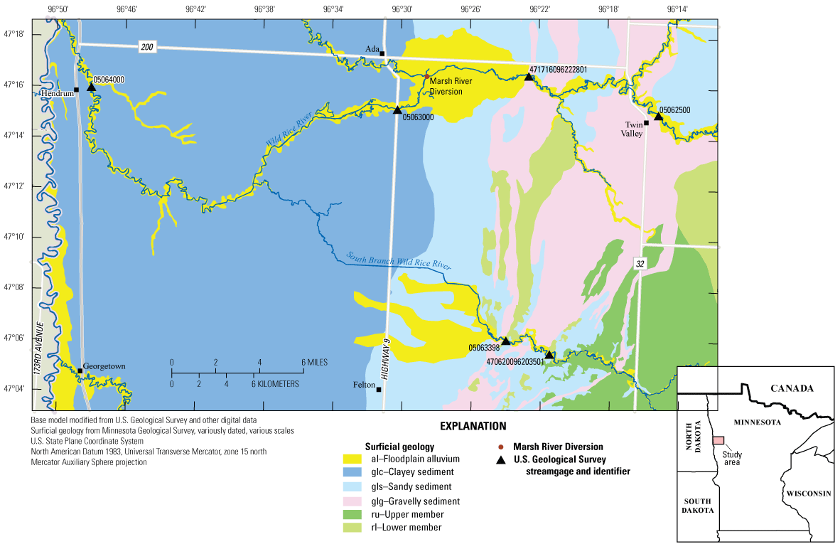
Map showing surficial geology and Marsh River Diversion near the Wild Rice River and South Branch Wild Rice River sampling sites.
Anthropogenic History
Land use within the basin has been heavily dominated by agricultural operations since the turn of the 20th century (Newkirk and others, 2017). Land use in the basin has changed more recently as row crops like corn and soybean varieties have replaced grasslands (Minnesota Groundwater Association, 2018). Additionally, a subsequent expansion of tile drainage throughout the state, in pursuit of higher row crop yields, has been aided by the preexisting surface drainage ditches in the basin (Minnesota Groundwater Association, 2018). Previous work by Schottler and others (2014) in Minnesota has shown that artificial drainage was the primary factor for an increase in streamflow, and climate and crop conversion explained less than one-half of the observed increase in streamflow.
Flooding
The Wild Rice River has a long history of major flooding, but minor flooding is also common. To help mitigate flooding, flood control measures and structures were built on the Wild Rice River in the 1950s from river mile 27 to 43 (Hendrickson, 2007). Flood control measures consisted of widening, deepening, and straightening the channel, and the WRWD constructed levees from the spoils of the straightened channels (Hendrickson, 2007). The Marsh River Diversion is a flood control structure on the Wild Rice River between sites Wild Rice River at County Road 2, Minnesota, (U.S. Geological Survey [USGS] station 471716096222801) and Wild Rice River near Ada, Minn. (USGS station 05063000; fig. 1).
The removal of natural meanders, to create a more uniform and straighter channel, resulted in an overall decrease of the river’s length (Hendrickson, 2007). These flood control measures and structures created a change in channel slope that altered system equilibrium by creating a knickpoint (Simon, 1989), which is defined as a sudden change in the river’s gradient and can be fixed or mobile. As the mobile knickpoint migrated upstream along the Wild Rice, it has created excess erosion and transport of sediment upstream and infilling of the channel downstream as the system attempts to return to equilibrium. Sediment deposition downstream of where the flood control structures are present has limited capacity for flood storage. Flood related damages are expensive. The most destructive flood year to date was 1997 with damages estimated at $100 to $150 million (Kjelland, 2001).
Hydrology and Sedimentology
The 30-year (1991 through 2020) mean annual precipitation ranges from 20 to 26 inches across the basin (Minnesota Department of Natural Resources State Climatology Office, 2021). The mean annual streamflow from water years 1945 through 2023 was 287 cubic feet per second (ft3/s) at the farthest downstream streamgage: Wild Rice River at Hendrum, Minn. (USGS station 05064000; U.S. Geological Survey, 2024). In 2006, the Minnesota Pollution Control Agency listed the lower reach of the Wild Rice River as impaired because of excess turbidity (Minnesota Pollution Control Agency, 2009). The impaired reach is located between the confluence with the South Branch of the Wild Rice River to the confluence with the Red River of the North, about 30 mi in total (Minnesota Pollution Control Agency, 2009). Various creeks and tributaries flowing into the Wild Rice River also have been designated as impaired since 2006. The latest designations were listed in 2018 (Minnesota Pollution Control Agency, 2024). The beach ridge is an easily erodible substrate, having unstable banks and a source that contributes substantial sediment to the Wild Rice River’s mainstem channel. As the Wild Rice River’s knickpoint migrates through this narrow but important source of sediment, it causes bank erosion and bed incision (Hendrickson, 2007). Brigham and others (2001) used radioisotopes to identify the Wild Rice River’s sediment sources. Their main findings were that upland soil erosion from cultivated fields contributes to most of the suspended-sediment concentration load (SSL) and that bank erosion is another contributor but not the dominant process for SSL. Brigham and others (2001) infer that even though bank erosion is not the dominant source of the SSL, it is an important contributor to the Wild Rice River’s bedload and the channel-forming processes.
Sampling Sites
Six USGS sampling sites were included in this study (table 1). The six sites were the Wild Rice River at Twin Valley, Minn. (USGS station 05062500; hereafter referred to as “Main Branch Upstream”), Wild Rice River at County Road 2, Minn. (USGS station 471716096222801; hereafter referred to as “Main Branch Middle”), Wild Rice River near Ada, Minn. (USGS station 05063000; hereafter referred to as “Main Branch Downstream”), South Branch Wild Rice River at 220th St., Minn. (USGS station 470620096203501; hereafter referred to as “South Branch Upstream”), South Branch Wild Rice River near Felton, Minn. (USGS station 05063398; hereafter referred to as “South Branch Downstream”), and Wild Rice River at Hendrum, Minn. (USGS station 05064000; hereafter referred to as “Outlet”). The six sites were sampled during different periods of record (table 1).
Table 1.
Site information for six sites in the Wild Rice River Basin.[Data are from U.S. Geological Survey (2024). Dates given in month/day/year format. USGS, U.S. Geological Survey; --, not available; MNDNR, Minnesota Department of Natural Resources]
A hypothesis prior to the study was that the sites on the same branch would have different sediment transport rates because the upstream sites (Main Branch Middle and South Branch Upstream) had higher gradients through the beach ridge, and the downstream sites (Main Branch Downstream and South Branch Downstream) had lower gradients closer to the lake plain. The USGS and WRWD picked these four sites to sample 8 to 10 times per year in WYs 2021–23 to determine if there were differences along and downstream of the beach ridge. Data had been collected for two of those sites (Main Branch Downstream and South Branch Downstream) as part of previous studies allowing comparison to the data collected in WYs 2021–23. The Main Branch Upstream, WYs 1993–2013, and Outlet, WYs 1979–2010, also had preexisting data to expand the study area extent.
Methods of Data Collection and Analysis
Samples were collected for a wide range of streamflows (fig. 3) during the ice-free season, which is generally from the end of March through November (open water season). The collected samples were analyzed for SSCs and percentage of fines, which were used to compute suspended-sands concentrations (hereafter referred to as “sands”) and suspended-fines concentrations (hereafter referred to as “fines”), total bedload mass, and bedload particle-size distributions. The laboratory analyses are described in the “Laboratory Methods” section.
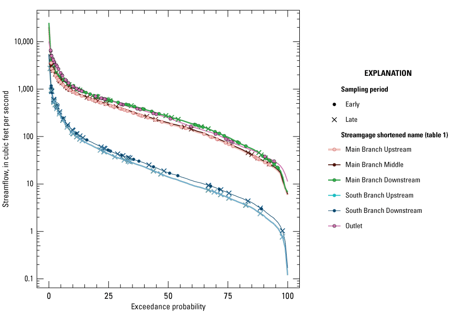
Graph showing flow duration curves for six Wild Rice River and South Branch Wild Rice River sampling sites and corresponding streamflows when suspended-sediment samples were collected.
Sampling Methods
Suspended-sediment samples were collected using isokinetic samplers and depth-integrating techniques at equal-width increments (EWIs; Edwards and Glysson, 1999; Davis and the Federal Interagency Sedimentation Project, 2005). For the collection of water samples, the river width was divided into 10 EWIs. An isokinetic, depth-integrated sample was collected at the centroid of each increment following procedures described in Edwards and Glysson (1999). Based on river depth and velocity, samples from each centroid were collected with a DH–48 sampler using a 1-pint glass bottle during wadable streamflows or a D–74 sampler with either a 1-pint or 1-quart glass bottle during nonwadable streamflows (Davis and the Federal Interagency Sedimentation Project, 2005). After the sampling event, the water samples collected from all the centroids of the river transect were combined into one composite sample for laboratory analyses.
Suspended-sediment sampling protocol changed between the first and second sampling periods of record. The protocol during the first period of record entailed touching the suspended-sediment sampler to the bottom of the channel when retrieving a sample. This sampling protocol might have led to possible contamination if the sampler inadvertently sampled a dune or the bottom of the channel, as was conveyed by the sampling staff (Chris Ellison, U.S. Geological Survey, written commun., 2023). During the second sampling period of record, sampling protocol was modified at all sites by testing the river’s depth prior to sampling and raising the sampler approximately 1 ft above the bottom of the channel to avoid contamination.
When bedload samples were collected, they were collected during the same sampling event as the SSC samples. Bedload sampling was attempted during every sampling event unless sampling equipment malfunctioned, or it was determined visually that bedload transport was not occurring. The visual determination of bedload transport occurring or not was at lower streamflows when the hydrologic technician was able to collect a wading sample and could see the river’s bottom. A BLH–84 pressure-differential bag sampler was used to collect bedload samples during wadeable streamflows, and a BL-84 was used during nonwadable streamflows (Davis and the Federal Interagency Sedimentation Project, 2005). The mesh pore sizes of the bags used to collect the bedload samples varied from 0.112 to 0.5 millimeter (mm), depending on site conditions. The single EWI method was used to collect bedload samples (Edwards and Glysson, 1999). Samples were collected by starting near one streambank and collecting one sample at each of the 20 evenly spaced increments across the stream cross-section to the opposite bank. The bedload sampler rested on the riverbed for 30 seconds at each increment. This process was repeated twice to obtain two separate samples. The minimum sample mass needed for laboratory analysis was 1.76 ounces and samples smaller than this amount were not sent to the laboratory for analyses. When samples were greater than the minimum sample mass, the samples from the bags were transferred into plastic containers and composited before laboratory analyses.
Laboratory Methods
Suspended-sediment samples were analyzed for SSC following method D3977–97 (Guy, 1969; American Society for Testing and Materials, 2000) and for the percentages of fines, by wet sieving (Guy, 1969), at the USGS Sediment Laboratory in Iowa City, Iowa. Fines are defined as particles with a diameter less than 0.0625 mm and consist of silt and clay. Particles that have a diameter greater than or equal to 0.0625 mm and as much as 2.0 mm are classified as sands. The sands were computed by taking the percentage of fines and multiplying it by the corresponding SSC value, dividing the product by 100 (eq. 1), and subtracting the fines from the SSC value (eq. 2):
whereFines
suspended-fines concentration, in milligrams per liter;
%Fines
percentage of fines in the SSC sample;
SSC
suspended-sediment concentration, in milligrams per liter; and
Sands
suspended-sands concentration, in milligrams per liter.
When “suspended-sediment constituents” is used in this report, it refers to SSCs which includes fines and sands.
Bedload samples were analyzed for total mass (grams) and particle-size classes using full phi sieves from 0.0625 to 16 mm and included 9 sizes (Guy, 1969). Bedload samples were analyzed at the USGS Sediment Laboratory in Iowa City, Iowa. Results from laboratory analyses can be accessed from the USGS National Water Information System (NWIS) database (U.S. Geological Survey, 2024). Bedload transport (BL) was computed using the following equation (Edwards and Glysson, 1999):
whereBL
is bedload transport, in tons per day;
K
is a conversion factor of 0.381 for the types of samplers used for data collection (BL–84 and BLH–84 have a 3-inch-wide opening);
W
is the total sampling width where the bedload samples were collected in the stream channel, in feet;
t
is total time the sampler was on the bed, in seconds; and
M
is total bedload mass of sample collected from all verticals sampled in the cross section, in grams.
Streamflow Data
Instantaneous (15-minute) streamflow data at the time of sediment sampling were obtained from co-located continuous streamgage records at the following sites: Main Branch Upstream, the South Branch Downstream, and the Outlet and are available from the NWIS database (U.S. Geological Survey, 2024). At sites without continuous streamflow records, concurrent streamflow measurements were made at most sampling events by the USGS at Main Branch Middle and South Branch Upstream and were made periodically by the Minnesota Department of Natural Resources (MNDNR) at Main Branch Downstream (Minnesota Department of Natural Resources, 2024). Regression analysis between the streamflow measurements and nearby streamgages were used to estimate streamflow during each sampling events without continuous streamflow records. The regressions were also used to estimate the continuous streamflow records at the sites without streamgages.
Estimating Streamflow at Ungaged Sites
Maintenance of Variance Extension Type 1 (MOVE.1) regression (Hirsch, 1982) analysis was used to relate concurrent streamflow measurements at the sampling locations without continuous streamflow records, Main Branch Middle, Main Branch Downstream, and South Branch Upstream, and a hydrologically similar index streamgage with a continuous record (fig. 4). The time of sampling was matched to the closest streamflow measurement at each location with a maximum time difference of 1 hour. The regression equation was then used to estimate streamflow during ungaged periods at the sampling location (table 2). Unlike ordinary least squares regression, which reduces the variance of estimated streamflows, the MOVE.1 regression equation has additional constraints to preserve the variance of the estimated streamflow, which produces less biased low- and high- streamflow estimates. MOVE.1 analyses were performed in R using the MOVE.1 function in the smwrStats package (Lorenz, 2022).
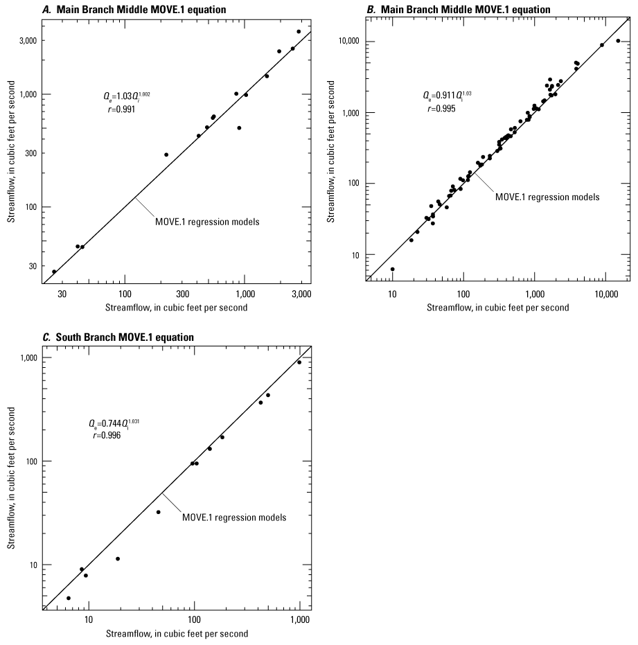
Line graphs showing the three Maintenance of Variance Extension Type 1 (MOVE.1) regressions with streamflow measurements at a ungaged location and streamflow at an index streamgage. A, Wild Rice River at County Road 2, Minnesota (U.S. Geological Survey [USGS] station 471716096222801) and Wild Rice River at Twin Valley, Minn. (USGS station 05062500). B, Wild Rice River near Ada, Minn. (USGS station 05063000) and USGS station 05062500. C, South Branch Wild Rice River at 220th St., Minn. (USGS station 470620096203501) and South Branch Wild Rice River near Felton, Minn. (USGS station 05063398).
Table 2.
Maintenance of Variance Extension Type 1 (MOVE.1) regression equations for three locations in the Wild Rice River Basin.[Data are from U.S. Geological Survey (2024). USGS, U.S. Geological Survey; Qe, streamflow estimate at ungaged site; Qi; streamflow value at index streamgage; r, Pearson correlation coefficient]
The Main Branch Upstream was used as an index streamgage for MOVE.1 streamflow estimates at the Main Branch Downstream and the Main Branch Middle. The South Branch Downstream was used as an index streamgage for streamflow estimates at the South Branch Upstream. Even though the Main Branch Downstream sampling site has a MNDNR streamgage, it does not have a complete and permanent record because the streamgage is operated as a temporary and provisional flood warning streamgage, and, prior to 2015, it was only operated during the open water season (Zachary Moore, MNDNR, written commun., 2023). All MOVE.1 relations between the index streamgages and streamflow measurements had Pearson correlation coefficients of greater than 0.99 (column “r” in table 2).
Rainfall Data
Rainfall data were available at four sites in the study area. Monthly rainfall data were downloaded from the National Oceanic and Atmospheric Administration Cooperative Observer Network from the following sites in Minnesota with station names Georgetown 1E, Ada, Halstad, and Mahnomen (National Oceanic and Atmospheric Administration, 2024). However, Halstad and Mahnomen had too much missing data and were not used. Ada and Georgetown (fig. 2) had fewer missing data and were plotted to compare rainfall between the two different periods of records when sediment sampling occurred at the South Branch Downstream. Straight line distances from rainfall sites are 19.4 miles between Georgetown and South Branch Downstream and 13.7 miles between Ada and South Branch Downstream.
Data Analysis
First, log-linear regressions were explored at each site to evaluate the relation between streamflow and SSC, sands, fines, and BL at each site. Log-linear regressions were in the form of equation 4, and log-linear regression equations can be transformed in the form of equation 5:
whereC
is the response variable and is either suspended-sediment concentration, in milligrams per liter; suspended-fines concentration, in milligrams per liter; suspended-sands concentration, in milligrams per liter; or bedload transport, in tons per day;
Q
is the explanatory variable streamflow, in cubic feet per second;
a and b
are fitted regression coefficients; and
BCF
is the bias-correction factor (Duan, 1983).
Residuals from regression in log-log space have a low bias when transformed back into arithmetic space. A bias correction factor (BCF), described by Duan (1983), was computed for each linear regression, applied to model predictions, and fitted values for computations in arithmetic space.
However, a nonconstant slope in the relation between log-transformed suspended-sediment constituents and streamflow was observed at all sampling sites after performing log-linear regression analysis. Piecewise regression was used to calculate the location of a breakpoint and fit a two-slope regression model for each sampling location and suspended-sediment constituents. A breakpoint is the value where there is a difference in slope coefficients (Muggeo, 2008). Piecewise regressions were fitted using the segmented package in R (Muggeo, 2008). Significance was tested by using each equation’s confidence interval. If the confidence interval contained zero, then the coefficient was not significantly different than zero.
Difference Testing
Sites with a first (WYs 2015 and before) and second (WYs 2021 through 2023) period of record (Main Branch Downstream and South Branch Downstream) used an indicator variable to test whether there was a significant difference in the SRCs during the two-sampling periods of record. The indicator variable was 0 for samples collected in the first period of record, and equal to 1 for samples during the second period of record. The indicator variable was added to equation 5 as an additional explanatory variable.
The Main Branch Middle and Main Branch Downstream sites are less than 8.5 river miles apart with a 1.3-percent difference between drainage areas. The South Branch Downstream and South Branch Upstream sites are less than 4 river miles apart with a 4.9-percent difference between drainage areas. To test if SRCs were different between each pair of sites, a site indicator variable was created that was equal to 1 for data from the downstream sites (Main Branch Downstream and South Branch Downstream) and 0 for data from the upstream sites (Main Branch Middle and South Branch Upstream) (Ramsey and Schafer, 1997). This site indicator variable was added as an explanatory variable to the regression equation (eq. 5). If the site indicator variable’s probability value (p-value) was greater than 0.05, the difference in the regression fits between the two sites on the same branch was not significant.
Daily and Annual Load Estimates
Daily SSLs and their upper and lower 95-percent prediction intervals were estimated using the following equation:
whereSSL
is the estimated suspended-sediment concentration load, in tons;
Q
is the daily mean streamflow, in cubic feet per second;
SSC
is the estimated daily mean suspended-sediment concentration from the piecewise regression models;
∆t
is the time step, in days; and
cf
is a coefficient (0.0027) that converts the units of streamflow and SSC into tons per day and assumes a specific gravity of 2.65 for sediment.
The SSLs and their upper and lower 95-percent prediction intervals were summed to compute annual loads for WYs 2021 through 2023 at the following four sites—Main Branch Middle, Main Branch Downstream, South Branch Upstream, and South Branch Downstream—to characterize differences and uncertainty in sediment transport among sites.
Streamflow, Suspended-Sediment Constituents, and Bedload Results
Summary statistics were calculated for streamflow, SSCs, sands, fines, and BL for the study area sites (table 3). Boxplots of streamflow, suspended-sediment constituents, and bedload are shown in figures 5, 6, and 7. Regarding BL specifically, the particle diameter representing the 50-percent cumulative percentile value (D50) was calculated at the sites where bedload samples collected: South Branch Upstream, South Branch Downstream, Main Branch Middle, and Main Branch Downstream (table 3). The bedload cumulative-frequency distribution of mean and range of particle sizes are shown in figure 8.
Table 3.
Summary statistics for six sites in the Wild Rice River Basin.[Data are from U.S. Geological Survey (2024). USGS, U.S. Geological Survey; StdDev, standard deviation; n, number of samples; --, not applicable; D50, 50-percent cumulative percentile value]
| Short name (table 1) |
USGS station number | Minimum | Maximum | Mean | Median | StdDev | n | D50 |
|---|---|---|---|---|---|---|---|---|
| Main Branch Upstream | 05062500 | 25 | 3,570 | 672 | 391 | 745 | 183 | -- |
| Main Branch Middle | 471716096222801 | 27 | 3,200 | 1,031 | 898 | 901 | 144 | -- |
| Main Branch Downstream | 05063000 | 22 | 4,061 | 898 | 682 | 873 | 358 | -- |
| South Branch Upstream | 470620096203501 | 1 | 2,784 | 297 | 67 | 610 | 102 | -- |
| South Branch Downstream | 05063398 | 1 | 2,770 | 271 | 60 | 483 | 169 | -- |
| Outlet | 05064000 | 30 | 6,550 | 1,454 | 637 | 1,668 | 93 | -- |
| Main Branch Upstream | 05062500 | 5 | 984 | 136 | 85 | 172 | 75 | -- |
| Main Branch Middle | 471716096222801 | 15 | 1,770 | 211 | 100 | 338 | 31 | -- |
| Main Branch Downstream | 05063000 | 6 | 1,140 | 218 | 121 | 256 | 90 | -- |
| South Branch Upstream | 470620096203501 | 2 | 259 | 33 | 13 | 54 | 32 | -- |
| South Branch Downstream | 05063398 | 2 | 2,070 | 112 | 19 | 304 | 56 | -- |
| Outlet | 05064000 | 28 | 792 | 166 | 117 | 144 | 45 | -- |
| Main Branch Upstream | 05062500 | 4 | 758 | 104 | 40 | 153 | 54 | -- |
| Main Branch Middle | 471716096222801 | 13 | 602 | 102 | 60 | 120 | 31 | -- |
| Main Branch Downstream | 05063000 | 5 | 980 | 144 | 65 | 192 | 86 | -- |
| South Branch Upstream | 470620096203501 | 2 | 186 | 26 | 8 | 43 | 32 | -- |
| South Branch Downstream | 05063398 | 2 | 408 | 43 | 13 | 80 | 51 | -- |
| Outlet | 05064000 | 26 | 427 | 122 | 98 | 91 | 24 | -- |
| Main Branch Upstream | 05062500 | 0.4 | 226 | 35 | 10 | 51 | 54 | -- |
| Main Branch Middle | 471716096222801 | 0.3 | 1,505 | 109 | 44 | 268 | 31 | -- |
| Main Branch Downstream | 05063000 | 0.5 | 387 | 77 | 44 | 91 | 86 | -- |
| South Branch Upstream | 470620096203501 | -- | 73 | 7 | 2 | 14 | 32 | -- |
| South Branch Downstream | 05063398 | -- | 307 | 27 | 4 | 64 | 51 | -- |
| Outlet | 05064000 | 1 | 47 | 8 | 6 | 9 | 24 | -- |
| Main Branch Middle | 471716096222801 | 1 | 287 | 79 | 30 | 85 | 51 | -- |
| Main Branch Downstream | 05063000 | 1 | 710 | 137 | 88 | 151 | 96 | -- |
| South Branch Upstream | 470620096203501 | 2 | 24 | 11 | 9 | 9 | 6 | -- |
| South Branch Downstream | 05063398 | 1 | 106 | 23 | 20 | 30 | 11 | -- |
| Main Branch Middle | 471716096222801 | -- | -- | -- | -- | -- | -- | 1.03 |
| Main Branch Downstream | 05063000 | -- | -- | -- | -- | -- | -- | 0.84 |
| South Branch Upstream | 470620096203501 | -- | -- | -- | -- | -- | -- | 0.85 |
| South Branch Downstream | 05063398 | -- | -- | -- | -- | -- | -- | 1.02 |
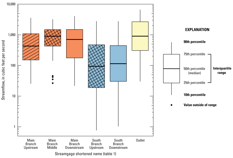
Boxplots showing streamflow for six sites in the Wild Rice River Basin.
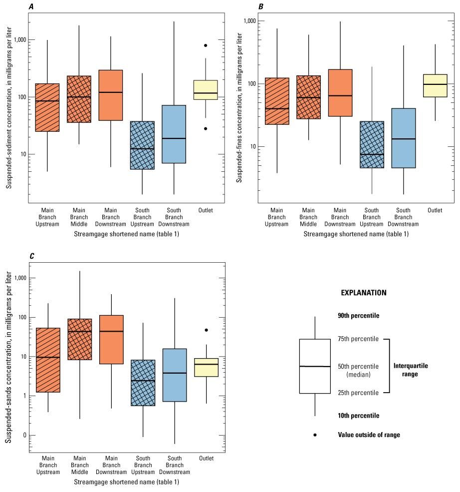
Boxplots showing suspended-sediment constituents for six sites in the Wild Rice River Basin. A, Suspended-sediment concentration. B, Suspended-fines concentration. C, Suspended-sands concentration.
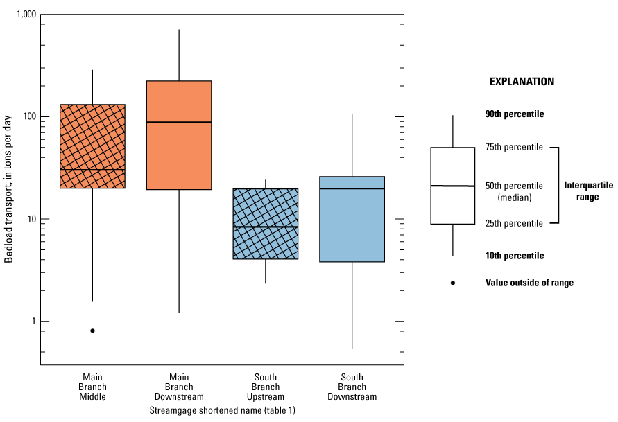
Boxplots showing bedload transport for four sites in the Wild Rice River Basin.
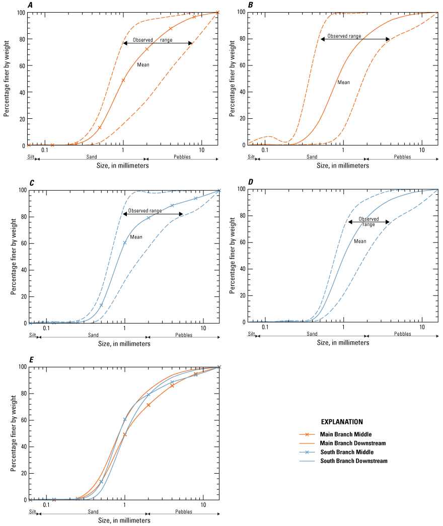
Line graphs showing cumulative-frequency distribution of mean and range of particle sizes in bedload samples for four sites in the Wild Rice River Basin. A, Wild Rice River at County Road 2, Minnesota (U.S. Geological Survey [USGS] station 471716096222801). B, Wild Rice River near Ada, Minn. (USGS station 05063000). C, South Branch Wild Rice River at 220th St., Minn. (USGS station 470620096203501). D, South Branch Wild Rice River near Felton, Minn. (USGS station 05063398).
Difference Testing
Samples collected from the Main Branch Downstream did not show a significant difference in the relations among suspended-sediment constituents and streamflow between the first and second period of record. However, a significant difference in the relations among streamflow and suspended-sediment constituents was observed at the South Branch Downstream between the first and second period of record. Piecewise regression models that were fitted using an indicator variable for the first and second period of record indicated a vertical offset for SSCs, sands, and fines. The site indicator variable used in the regression equations was not significant for SSCs, fines, and sands for both pairs of sites. The site indicator variable was significant in the Main Branch BL regression equation.
Regression Models and Loads
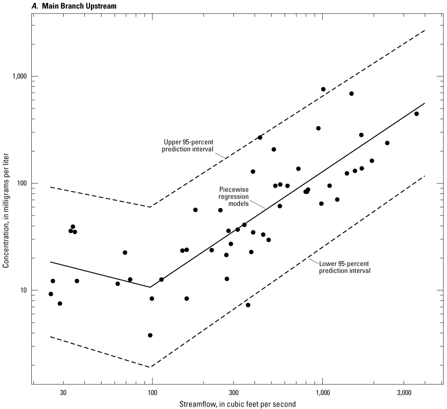
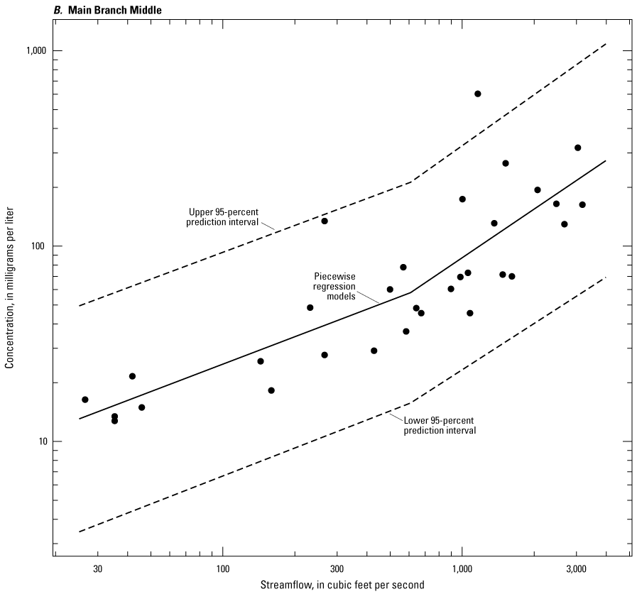
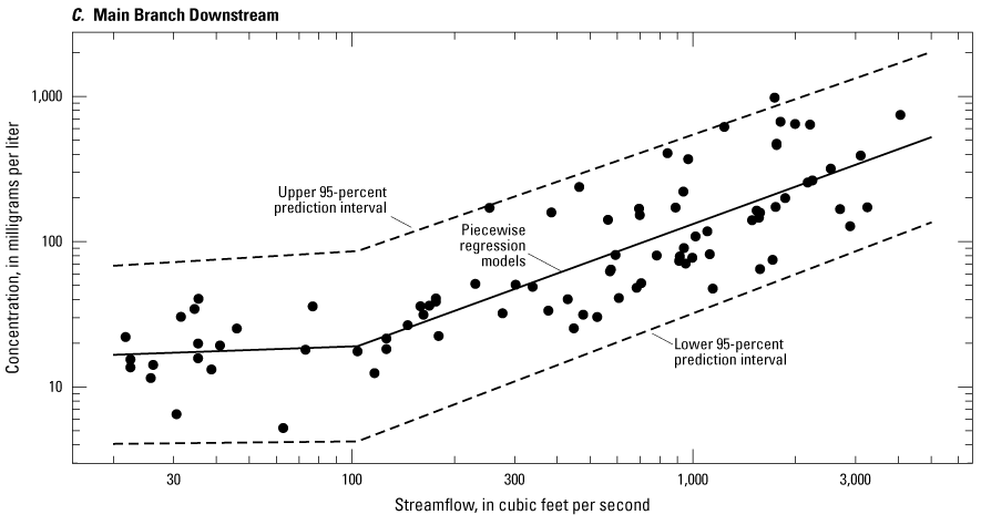
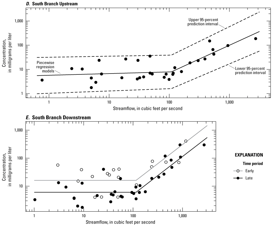
Piecewise regression equations were developed for each of the Wild Rice River sites for suspended-sediment constituents (figs. 9–11; table 4). The piecewise regression models were developed to estimate SSCs, sands, and fines for each of the six locations. The R2 for all suspended-sediment constituents improved from log-linear regressions to piecewise regressions at all six locations. Log-linear BL regression models (fig. 12) were developed for the Main Branch Middle, Main Branch Downstream, and South Branch Downstream, but there was not enough data to develop a model at the South Branch Upstream.
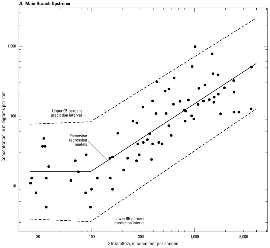
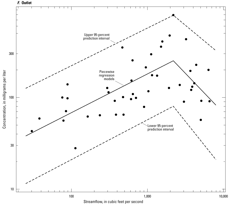
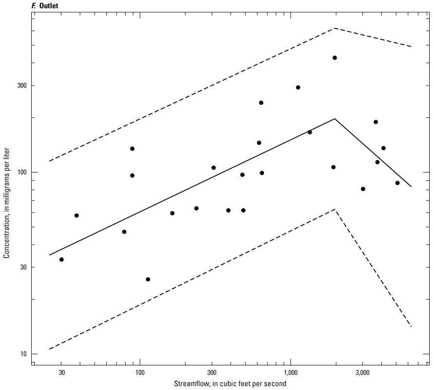
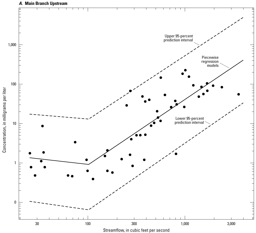
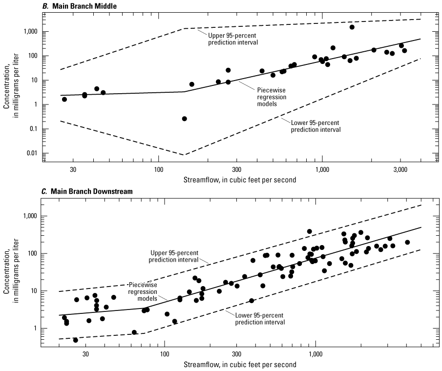
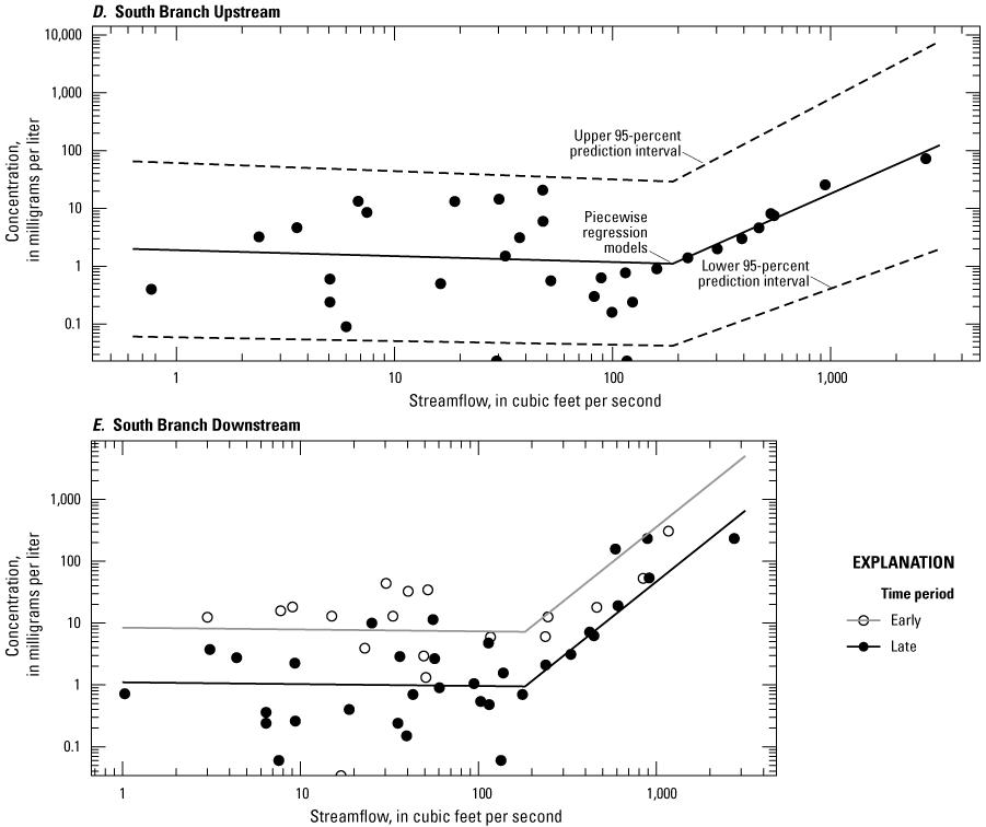
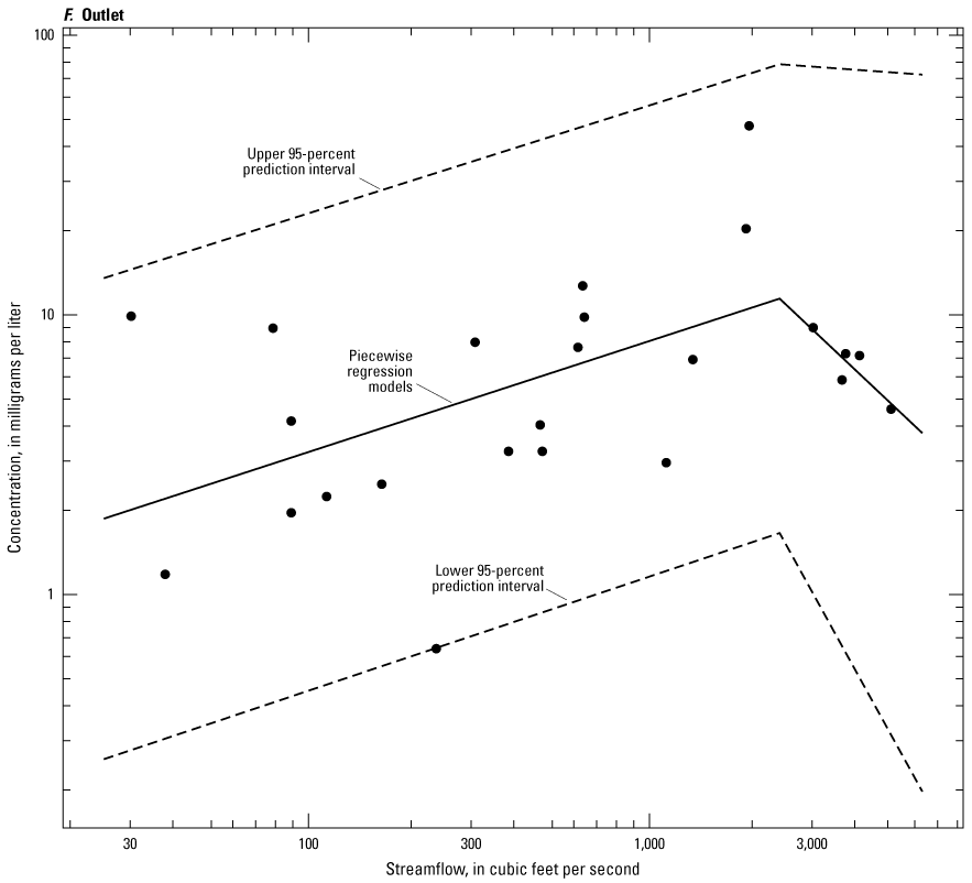
Scatterplots showing piecewise suspended-sediment concentration (SSC) regression models for six locations in the Wild Rice River Basin. A, Wild Rice River at Twin Valley, Minnesota (U.S. Geological Survey [USGS] station 05062500). B, Wild Rice River at County Road 2, Minn. (USGS station 471716096222801). C, Wild Rice River near Ada, Minn. (USGS station 05063000). D, South Branch Wild Rice River at 220th St., Minn. (USGS station 470620096203501). E, South Branch Wild Rice River near Felton, Minn. (USGS station 05063398). F, Wild Rice River at Hendrum, Minn. (USGS station 05064000).
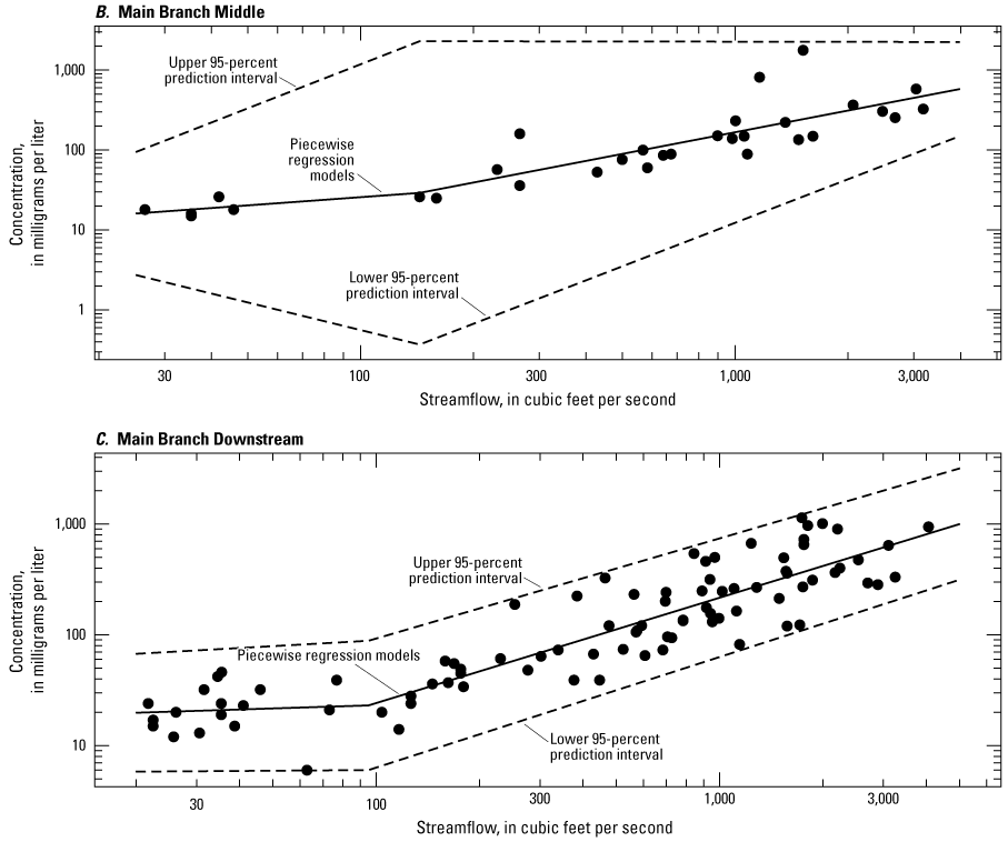
Scatterplots showing piecewise suspended-fines concentration (Fines) regression models for six locations in the Wild Rice River Basin. A, Wild Rice River at Twin Valley, Minnesota (U.S. Geological Survey [USGS] station 05062500). B, Wild Rice River at County Road 2, Minn. (USGS station 471716096222801). C, Wild Rice River near Ada, Minn. (USGS station 05063000). D, South Branch Wild Rice River at 220th St., Minn. (USGS station 470620096203501). E, South Branch Wild Rice River near Felton, Minn. (USGS station 05063398). F, Wild Rice River at Hendrum, Minn. (USGS station 05064000).
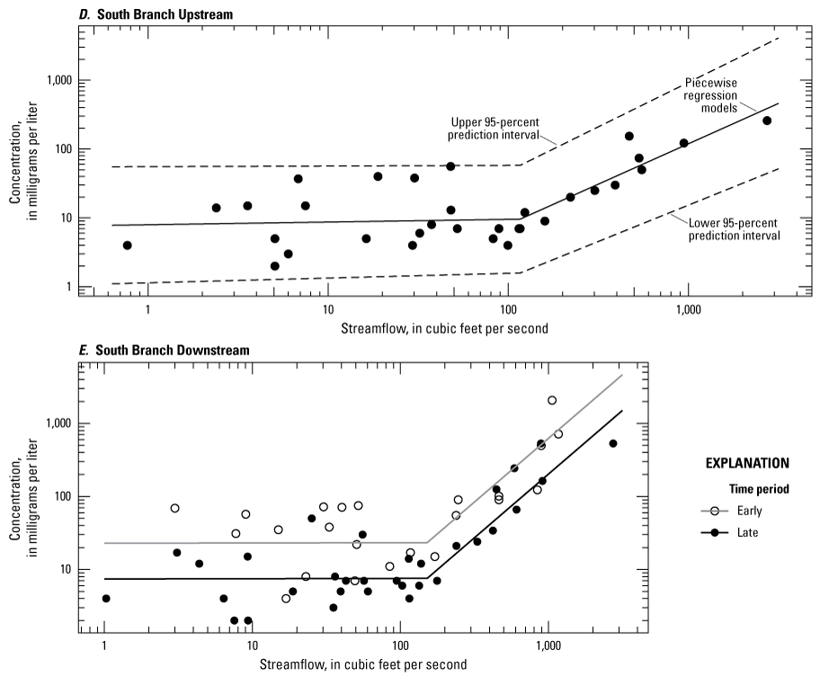
Scatterplots showing piecewise suspended-sands concentration (Sands) regression models for six locations in the Wild Rice River Basin. A, Wild Rice River at Twin Valley, Minnesota (U.S. Geological Survey [USGS] station 05062500). B, Wild Rice River at County Road 2, Minn. (USGS station 471716096222801). C, Wild Rice River near Ada, Minn. (USGS station 05063000). D, South Branch Wild Rice River at 220th St., Minn. (USGS station 470620096203501). E, South Branch Wild Rice River near Felton, Minn. (USGS station 05063398). F, Wild Rice River at Hendrum, Minn. (USGS station 05064000).
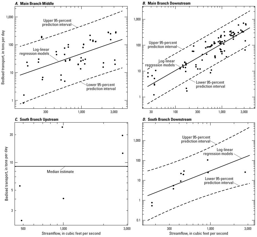
Scatterplots showing the bedload transport (BL) regression models for four locations in the Wild Rice River Basin. A, Log-linear BL for Wild Rice River at County Road 2, Minnesota (U.S. Geological Survey [USGS] station 471716096222801). B, Log-linear BL Wild Rice River near Ada, Minn. (USGS station 05063000). C, Median BL estimate for South Branch Wild Rice River at 220th St., Minn. (USGS station 470620096203501). D, Log-linear BL for South Branch Wild Rice River near Felton, Minn. (USGS station 05063398).
The suspended-sediment constituents’ regressions with their upper and lower 95-percent prediction intervals are shown in figures 9–11, and the regression equations are in table 4. There are two equations for each location. “Lower piecewise regression equation” refers to the equation at lower streamflows and “Upper piecewise regression equation” refers to the equation at higher streamflows.” The column titled “Breakpoint streamflow” is the breakpoint location (table 4). For suspended-sediment constituent regression equations developed at lower streamflows (less than or equal to the breakpoint), most had coefficients that were not significantly different than zero (table 4); however, all suspended-sediment constituents for the Outlet and fines in the Main Branch Middle were significantly different than zero at lower streamflows. For suspended-sediment constituent regression equations developed at higher streamflows, most had coefficients that were significantly different than zero between streamflow and the constituent except at the Outlet for all suspended-sediment constituents.
Table 4.
Regression equations for six locations in the Wild Rice River Basin.[Data are from U.S. Geological Survey (2024). See table 1 for full site information. R2, coefficient of determination; ft3/s, cubic feet per second; minimum streamflow, minimum streamflow when bedload sample was collected; SSC, suspended-sediment concentration; Q, streamflow; --, not applicable; fines, suspended-fines concentration; sands, suspended-sands concentration; BL, bedload transport]
| Short name (table 1) |
R2 | Breakpoint streamflow (ft3/s) |
Lower piecewise regression equation, used at less than or equal to breakpoint streamflow | Upper piecewise regression equation, used at greater than breakpoint streamflow | Minimum streamflow (ft3/s) |
Bedload equation, used at greater than or equal to minimum streamflow |
|---|---|---|---|---|---|---|
| Main Branch Upstream | 0.69 | 97 | SSC=16.2Q−0.002×1.32a | SSC=0.199Q0.959×1.32 | -- | -- |
| Main Branch Middle | 0.77 | 144 | SSC=5.36Q0.341×1.31a,b | SSC=0.333Q0.900×1.31b | -- | -- |
| Main Branch Downstream | 0.81 | 95 | SSC=14.8Q0.098×1.18a,b | SSC=0.304Q0.951×1.18b | -- | -- |
| South Branch Upstream | 0.59 | 116 | SSC=7.96Q0.039×1.46a,b | SSC=0.036Q1.17×1.46b | -- | -- |
| South Branch Downstream Early | 0.75 | 152 | SSC=22.8Q0.004×1.4a | SSC=0.004Q1.74×1.4 | -- | -- |
| South Branch Downstream Late | 0.75 | 152 | SSC=7.41Q0.004×1.4a,b | SSC=0.0012Q1.74×1.4b | -- | -- |
| Outlet | 0.43 | 2,190 | SSC=9.75Q0.423×1.17 | SSC=194,133Q−0.864×1.17a | -- | -- |
| Main Branch Upstream | 0.68 | 97 | Fines=67.5Q−0.403×1.33a | Fines=0.081Q1.07×1.33 | -- | -- |
| Main Branch Middle | 0.70 | 609 | Fines=2.90Q0.467×1.25 | Fines=0.286Q0.828×1.25 | -- | -- |
| Main Branch Downstream | 0.71 | 104 | Fines=13.0Q0.083×1.26a | Fines=0.361Q0.855×1.26 | -- | -- |
| South Branch Upstream | 0.66 | 109 | Fines=5.70Q0.069×1.35a | Fines=0.038Q1.14×1.35 | -- | -- |
| South Branch Downstream Early | 0.71 | 115 | Fines=16.1Q0.00×1.34a | Fines=0.025Q1.36×1.34 | -- | -- |
| South Branch Downstream Late | 0.71 | 115 | Fines=6.04Q0.00×.34a | Fines=0.0095Q1.36×1.34 | -- | -- |
| Outlet | 0.48 | 1960 | Fines=9.76Q0.396×1.16 | Fines=52,216Q−0.736×1.16a | -- | -- |
| Main Branch Upstream | 0.68 | 102 | Sands=3.34Q−0.280×1.95a | Sands=0.0004Q1.66×1.95 | -- | -- |
| Main Branch Middle | 0.81 | 143 | Sands=1.28Q0.191×1.52a | Sands=0.002Q1.50×1.52 | -- | -- |
| Main Branch Downstream | 0.85 | 73 | Sands=0.822Q0.334×1.24a | Sands=0.022Q1.18×1.24 | -- | -- |
| South Branch Upstream | 0.32 | 189 | Sands=1.90Q-0.103×2.61a | Sands=0.0002Q1.67×2.61 | -- | -- |
| South Branch Downstream Early | 0.65 | 183 | Sands=8.44Q−0.030×2.09a | Sands=0.00005Q2.30×2.09 | -- | -- |
| South Branch Downstream Late | 0.65 | 183 | Sands=1.10Q−0.030×2.09a | Sands=0.000006Q2.30×2.09 | -- | -- |
| Outlet | 0.26 | 2,408 | Sands=0.519Q0.397×1.41 | Sands=87,660Q−1.15×1.41a | -- | -- |
| Main Branch Middle | 0.31 | -- | -- | -- | 142 | BL=0.128Q0.857×1.81 |
| Main Branch Downstream | 0.75 | -- | -- | -- | 26 | BL=0.091Q1.03×1.25 |
| South Branch Upstream | -- | -- | -- | -- | 472 | BL=9 |
| South Branch Downstream | 0.57 | -- | -- | -- | 180 | BL=0.001Q1.56×1.69 |
For estimating the suspended-sediment constituent at streamflows less than or equal to the breakpoint, use the “Lower piecewise regression equation” in table 4. For estimating the constituent at streamflows greater than the breakpoint, use the “Upper piecewise regression equation” in table 4. Even though coefficients were not significant at certain sites and streamflows (table 4), their equations were retained to maintain consistency in predictions across the entire range of streamflow. Also, the piecewise equations, as fit, provide unbiased estimates across the whole streamflow regime.
For estimating BL at streamflows greater than or equal to the minimum streamflow when bedload samples were collected, use the “Bedload equation” in table 4. There were not enough samples to develop a log-linear regression equation at South Branch Upstream, so the BL estimate is the median value of the sampled data, “Bedload equation” in table 4. At streamflows less than or equal to the minimum streamflow when bedload samples were collected, there is no BL estimate because BL was not observed at these streamflows.
Annual SSL and upper and lower 95-percent prediction intervals were calculated in R from daily streamflows and SSC estimates from the “Lower piecewise regression equation” and “Upper piecewise regression equation” (table 4) at the Main Branch Middle, Main Branch Downstream, South Branch Upstream, and South Branch Downstream for WYs 2021 through 2023 (fig. 13; table 5). Mostly, SSLs were higher at the downstream sites on the same branch. Also, SSLs loads were higher on the Main Branch sites than the South Branch sites.
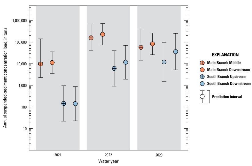
Annual suspended-sediment concentration loads and upper and lower 95-percent prediction intervals at four Wild Rice River Main and South Branch sites, water years 2021 through 2023.
Table 5.
Annual suspended-sediment concentration loads and upper and lower 95-percent prediction intervals at four Wild Rice River Main and South Branch sites, water years 2021 through 2023.[Data are from U.S. Geological Survey (2024). See table 1 for full site information]
| Short name (table 1) |
Lower 95-percent prediction interval | Suspended-sediment concentration load | Upper 95-percent prediction interval |
|---|---|---|---|
| Main Branch Middle | 2,308 | 9,595 | 141,138 |
| Main Branch Downstream | 3,559 | 11,195 | 35,387 |
| South Branch Upstream | 22 | 145 | 957 |
| South Branch Downstream | 23 | 141 | 878 |
| Main Branch Middle | 41,573 | 156,654 | 688,670 |
| Main Branch Downstream | 72,429 | 226,980 | 711,584 |
| South Branch Upstream | 916 | 6,002 | 39,640 |
| South Branch Downstream | 1,901 | 11,554 | 70,452 |
| Main Branch Middle | 14,449 | 56,734 | 396,946 |
| Main Branch Downstream | 26,063 | 82,341 | 260,469 |
| South Branch Upstream | 1,473 | 11,876 | 96,923 |
| South Branch Downstream | 5,172 | 36,071 | 252,406 |
Discussion
Generally, data distributions of suspended-sediment constituents and bedload are more similar on the same branch and values are less along the South Branch and Outlet sites than the Main Branch sites (figs. 6–7). However, the data demonstrate substantial variability in sediment transport that is affected by many factors such as different sediment sources; sediment supply; rate of erosion; phases of sediment transport; sediment deposition; antecedent conditions; and magnitude, intensity, and duration of storm events. Even though these data indicate constituents were higher or lower at certain sites, it is not expected that this is always the case. Because there were different sampling periods and some sites had more samples collected than others, this, in part, might explain the variability.
Bedload samples could not be collected at lower streamflows like suspended-sediment samples because bedload transport does not occur at lower streamflow velocities. In alluvial streams like the Wild Rice River, there is a functional relation among the hydraulic properties of streamflow and suspended sands and bedload; however, there is not a functional relation between suspended fines (wash load) and streamflow. Sand can either be transported in multiple phases as bedload and (or) suspended by turbulent flow. The transport rate of suspended fines is usually a function of the supply made available and does not need turbulent flow for transport. Suspended fines are normally delivered to the stream by overland flow, tile drains, bank sloughing, and (or) bank erosion. For this study, a log-linear relation between BL and streamflow was significant at the Middle Branch Downstream, Middle Branch Upstream, and South Branch Downstream, whereas piecewise regression was not significant for BL because the breakpoint did not represent an actual change in sediment transport. Fewer bedload samples were collected at the South Branch sites because these sites have less streamflow and are flashier than the Main Branch sites. The minimum streamflow when bedload samples were collected at the South Branch Upstream was 472 ft3/s and the South Branch Downstream was 180 ft3/s with exceedance probabilities of 2.5 and 7.7 percent, respectively (fig. 3). However, bedload can be highly variable. For example, bedload was attempted at a higher streamflow of 245 ft3/s at the South Branch Downstream but yielded no sample on April 23, 2023, because ice on top of the river melted 10 days prior, and the streambed may have still been frozen or partially frozen.
A significant difference was observed at the South Branch Downstream in the streamflow and SSC relation between the first and second period of record; however, Warrick (2015) cautions that apparent changes in the streamflow and SSC relation do not necessarily indicate a change in sediment transport but could be caused by several different factors. In this scenario, the difference in the relation for first and second period of record at the South Branch may be partially attributed to differences in the sampling events between these two periods. Histograms of the number of samples collected per month at the South Branch location during the first and second period of record are shown in figure 14. The histograms are substantially different between the two time periods. More months were sampled during the first sampling period of record, including March and November (fig. 14A). Most of the samples for the second period of record were collected during April, May, and June (fig. 14B). Antecedent conditions (more wet conditions in the second period of record) might explain the difference between these two periods rather than an actual change in sediment transport. The later sampling period occurred over a three-year period, and few samples were collected in 2021 because of dry conditions. Sampling in 2022 and 2023 required targeting wet conditions in the spring and early summer to get the required number of samples for this study. Another possible explanation for the differences might, in part, be attributed to a change in the suspended-sediment sampling methods between the first and second periods of record.
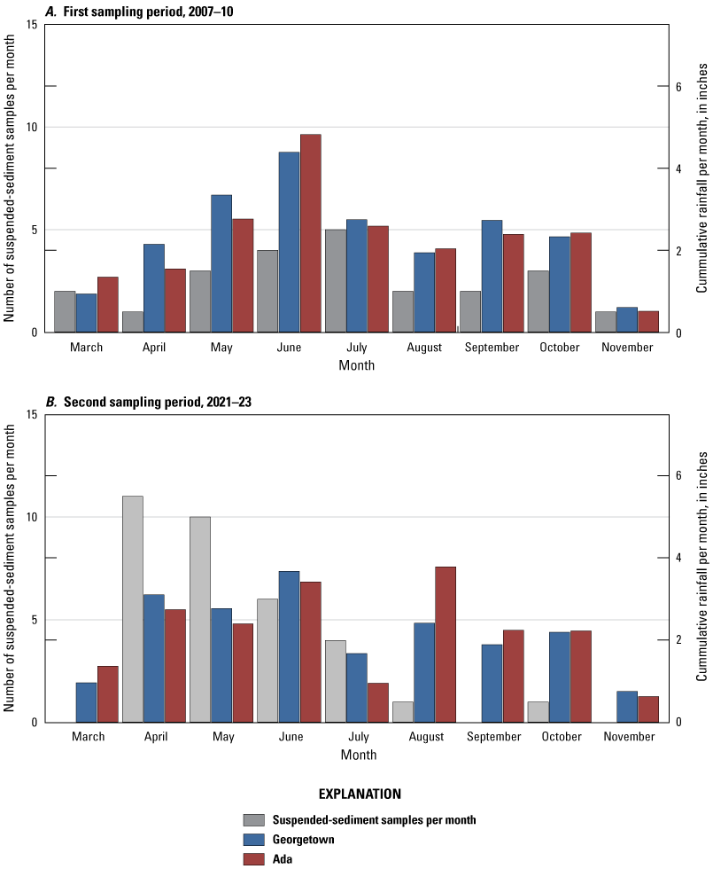
Histograms showing the number of samples per month at the South Branch Wild Rice River near Felton, Minnesota (U.S. Geological Survey [USGS] station 05063398) during two sampling periods, and cumulative monthly rainfall at Georgetown and Ada, Minn. A, The first period of record included samples collected water years 2007 through 2010. B, The second period of record included samples collected water years 2021 through 2023.
Overall, piecewise regression models fit the actual sediment transport process better for suspended-sediment constituents by differentiating between streamflow and the suspended-sediment constituent no relations and (or) relations at lower and higher streamflows. This differentiating of relations at lower and higher streamflows was an alternative approach from previous studies that just used one relation to explain SSC predictions from streamflow (Ellison and others, 2014, 2016). Most sites did not have a relation between streamflow and the suspended-sediment constituent at lower streamflows except the Outlet for all suspended-sediment constituents and for fines at the Main Branch Middle. All the streamflow and suspended-sediment constituent relations, except the Outlet, were significant at higher streamflows. The negative relations at the Outlet during higher streamflows provide evidence to support that the lower Wild Rice River is supply limited and deposition is likely occurring upstream and (or) near this site. This is substantiated by the presence of lower velocities during higher streamflows because the gradient is lowest in this area of the basin and likely affected by backwater conditions when the Red River of the North is flooding. The breakpoints identified in piecewise regression can be caused by different dominant processes such as sediment supply, transport processes, and deposition at different streamflow regimes.
A hypothesis prior to the study was that sites on the same branch would have different sediment transport rates because the upstream sites (Main Branch Middle and South Branch Upstream) had higher gradients through the beach ridge, compared to the downstream sites (Main Branch Downstream and South Branch Downstream), which had lower gradients closer to the lake plain. However, the suspended-sediment constituents were not statistically different between these sites on the same branch after performing difference testing; however, there is a great deal of uncertainty when using streamflow as an explanatory variable and even greater uncertainty when estimating streamflow if a continuous streamgage is not present. There were three sites in this study that used estimated streamflow, and future efforts could benefit from more continuous streamflow records along the Wild Rice Main and South Branches. Also, the Marsh River Diversion on the Main Branch (fig. 2) is another cause of uncertainty because at higher streamflows the Wild Rice is diverting into the diversion. In 1988, the U.S. Army Corps of Engineers (1988) estimated that the Wild Rice River began diverting into the Marsh River Diversion when the Wild Rice was greater than 4,000 ft3/s (U.S. Army Corps of Engineers, 1988). Since the knickpoint has lowered the baselevel of the Wild Rice River, the streamflow capacity of the channel has become greater than 4,000 ft3/s, and the streamflow value is now unknown when it starts to divert into the Marsh River (Jerry Bents, Houston Engineering, written commun., 2024). In most streams, sediment transport and streamflow are not independent of one another, so it can be challenging to differentiate upstream changes in sediment supply from variability in streamflow year-to-year (Warrick, 2015). Even though there was no detectable difference, given the large uncertainty, the scale of difference required to detect would need to be large, so the difference testing used is not particularly sensitive or a powerful test.
Given the large uncertainty when difference testing, SSLs and upper and lower 95-percent prediction intervals were calculated for the four sites sampled in WYs 2021 through 2023 to look at differences among these sites and quantify uncertainty. Overall, the piecewise regression equations used to calculate SSLs for the Main Branch Middle and Main Branch Downstream were similar to each other and the South Branch Upstream and South Branch Downstream were also similar to each other. SSLs were higher at the downstream sites on the same branch compared to their respective upstream site from year to year. Also, even though the piecewise regression slopes were greater at the South Branch sites than the Main Branch sites, the SSL were higher at the Main Branch sites because streamflow was higher at these sites. The prediction intervals at each site had a large range that provided an estimate for uncertainty, and there is considerable overlap between the sites’ prediction intervals on the same branch. For example, the upper 95-percent SSL prediction interval was higher at the Main Branch Middle than the Main Branch Downstream in WYs 2021 and 2023 and was higher at the South Branch Upstream than the South Branch Downstream in WY 2021, which suggests SSLs could be higher through the beach ridge during certain time periods, but, because of the large uncertainty, a final determination of differences between sites cannot be made, only inferred, from the data and results.
Variability among sites and periods of record might be due to the timing of sampling, modification of sampling procedures, the number of samples collected, and the uncertainty of using streamflow as the sole explanatory variable. Sediment transport is exacerbated by the presence of the knickpoint, which continues to induce erosion as the system tries to reach equilibrium. Continued monitoring could help inform the future restoration design and monitor the system after the future restoration has been completed. Turbidity as a surrogate for SSC was more promising than just using streamflow as a sole explanatory variable at select Wild Rice River sites in a previous study (Ellison and others, 2014). Oftentimes, in situ sensors, such as turbidity and acoustics, are more accurate at predicting suspended sediment than just using streamflow (Rasmussen and others, 2009; Landers and others, 2016; Topping and Wright, 2016); however, purchasing and maintaining sensors can be expensive. Since turbidity showed promise in a previous study that included Wild Rice sites (Ellison and others, 2014) and acoustics worked in another part of Minnesota (Groten and others, 2019), turbidity and acoustics could be explored if future monitoring efforts continue.
Summary and Conclusions
The Wild Rice River continues to experience major morphological adjustments because of its geologic history and anthropogenic modifications. Flood control measures constructed in the Wild Rice River during the middle of the 20th century created a mobile knickpoint that causes erosion and excess fluvial sediment transport, and the excess sediment eventually deposits in the lower Wild Rice River, which exacerbates flooding. To help mitigate these problems and help accelerate the river to reach equilibrium, the Wild Rice Watershed District (WRWD) has future plans of implementing a river restoration on the lower Wild Rice River by setting flood levees back, widening the river corridor, and reconstructing meanders in the channel. The WRWD, in collaboration with the U.S. Geological Survey, measured and analyzed sediment transport along the Wild Rice’s Main and South Branches to assess potential changes in sediment transport among sites and two periods of record, 2015 and prior and 2021 through 2023, which could help inform future river restoration designs.
Time differencing results indicated all suspended-sediment constituents had a significant difference between the two sampling periods at one South Branch site but not at the Main Branch site, which could be possibly explained from a change in sediment supply, transport processes, a difference in sampling procedures, or from a combination of factors. Regression analysis was used to provide estimates of suspended-sediment constituents and bedload when samples were unable to be collected. Piecewise regression analysis better matched the suspended-sediment constituents transport process at most sites by differentiating between relations at lower and higher streamflows. Five of the sites showed elevated sediment transport with increasing streamflow, whereas the site furthest downstream showed a negative relation with increasing streamflow, indicating that the lower Wild Rice River is supply-limited and depositions are likely occurring upstream and (or) near the site. Site differencing results indicated data collected from two Main Branch sites and two South Branch sites had no detectable difference but, given the large uncertainty in the results, the test used was not particularly sensitive or a powerful test. Therefore, suspended-sediment concentration loads (SSLs) and prediction intervals were computed and compared amongst the two Main Branch and two South Branch sites. The SSLs were higher at the downstream sites and at the Main Branch sites than at the South Branch sites. However, the upper 95-percent SSL prediction interval was higher during certain water years at the Main Branch Middle and the South Branch Upstream than at the Main Branch Downstream and South Branch, respectively, which suggests SSLs could be higher through the beach ridge. But, because of the large uncertainty, a final determination of differences between sites cannot be made, only inferred, from the data and results. Overall, the uncertainty observed in the results demonstrated the complexity of sediment transport in a river when using streamflow as the sole explanatory variable and suggests a need for multisite, multiyear, and multifaceted data such as using in situ continuous measures of turbidity and (or) acoustics, which might provide more accurate estimates of sediment transport.
References Cited
American Society for Testing and Materials, 2000, Standard test methods for determining sediment concentration in water samples: West Conshohocken, Pa., American Society for Testing and Materials International, D3977–97, v.11.02, 3 p., accessed August 2024 at https://cdn.standards.iteh.ai/samples/12289/323e853a53cb4bb78bab127545c97cf0/ASTM-D3977-97.pdf.
Brigham, M.E., McCullough, C.J., and Wilkinson, P.M., 2001, Analysis of suspended-sediment concentrations and radioisotope levels in the Wild Rice River Basin, northwestern Minnesota, 1973–98: U.S. Geological Survey Water Resources Investigations Report 2001–4192, 21 p., accessed August 2024 at https://doi.org/10.3133/wri014192.
Barry, J.J., Buffington, J.M., Goodwin, P., King, J.G., and Emmett, W.W., 2008, Performance of bed-load transport equations relative to geomorphic significance—Predicting effective discharge and its transport rate: Journal of Hydraulic Engineering (New York, N.Y.), v. 134, no. 5, p. 601–615, accessed August 2024 at https://doi.org/10.1061/(ASCE)0733-9429(2008)134:5(601).
Bluemle, J.P., 2024, Glacial Lake Agassiz: North Dakota Geological Survey web page accessed May 30, 2024, at https://www.dmr.nd.gov/ndgs/ndnotes/agassiz/.
Davis, B.E., and the Federal Interagency Sedimentation Project, 2005, A guide to the proper selection and use of federally approved sediment and water-quality samplers: U.S. Geological Survey Open-File Report 2005–1087, 20 p. [Also available at https://doi.org/10.3133/ofr20051087.]
Duan, N., 1983, Smearing estimate—A nonparametric retransformation method: Journal of the American Statistical Association, v. 78, no. 383, p. 605–610, accessed August 2024 at https://doi.org/10.1080/01621459.1983.10478017.
Edwards, T.K., and Glysson, G.D., 1999, Field methods for measurement of fluvial sediment: U.S. Geological Survey Techniques of Water-Resources Investigations, book 3, chap. C2, 89 p. [Also available at https://pubs.usgs.gov/twri/twri3-c2/.]
Ellison, C.A., Groten, J.T., Lorenz, D.L., and Koller, K.S., 2016, Application of dimensionless sediment rating curves to predict suspended-sediment concentrations, bedload, and annual sediment loads for rivers in Minnesota (ver. 1.1, January 2020): U.S. Geological Survey Scientific Investigations Report 2016–5146, 68 p., accessed August 2024 at https://doi.org/10.3133/sir20165146.
Ellison, C.A., Savage, B.E., and Johnson, G.D., 2014, Suspended-sediment concentrations, loads, total suspended solids, turbidity, and particle-size fractions for selected rivers in Minnesota, 2007 through 2011: U.S. Geological Survey Scientific Investigations Report 2013–5205, 43 p., accessed August 2024 at https://doi.org/10.3133/sir20135205.
Gellis, A.C., 2013, Factors influencing storm-generated suspended-sediment concentrations and loads in four basins of contrasting land use, humid-tropical Puerto Rico: Catena, v. 104, p. 39–57, accessed August 2024 at https://doi.org/10.1016/j.catena.2012.10.018.
Groten, J.T., Ziegeweid, J.R., Lund, J.W., Ellison, C.A., Costa, S.B., Coenen, E.N., and Kessler, E.W., 2019, Using acoustic Doppler velocity meters to estimate suspended sediment along the lower Minnesota and Mississippi Rivers: U.S. Geological Survey Scientific Investigations Report 2018–5165, 30 p., accessed August 2024 at https://doi.org/10.3133/sir20185165.
Guy, H.P., 1969, Laboratory theory and methods for sediment analysis: U.S. Geological Survey Techniques of Water Resources Investigations, book 5, chap. C1, 58 p. [Also available at https://pubs.usgs.gov/twri/twri5c1/.]
Hirsch, R.M., 1982, A comparison of four streamflow record extension techniques: Water Resources Research, v. 18, no. 4, p. 1081–1088, accessed August 2024 at https://doi.org/10.1029/WR018i004p01081.
Hobbs, H.C., and Goebel, J.E., 1982, S-01 Geologic map of Minnesota, quaternary geology: Minnesota Geological Survey, 1 sheet, scale 1:500,000, accessed July 25, 2024, at https://hdl.handle.net/11299/60085.
Kjelland, M.E., 2001, Quantification of historic flood damage in the Maple and Wild Rice watersheds of the Red River of the North Basin: accessed September 4, 2023, at https://www.academia.edu/53714917/Quantification_of_historic_flood_damage_in_the_Maple_and_Wild_Rice_watersheds_of_the_Red_River_of_the_North_Basin.
Landers, M.N., Straub, T.D., Wood, M.S., and Domanski, M.M., 2016, Sediment acoustic index method for computing continuous suspended-sediment concentrations: U.S. Geological Survey Techniques and Methods, book 3, chap. C5, 63 p. [Also available at https://doi.org/10.3133/tm3C5.]
Lopes, V.L., Osterkamp, W.R., and Bravo-Espinosa, M., 2001, Evaluation of selected bedload equation under transport- and supply-limited conditions, in Proc. Seventh Interagency Sedimentation Conference, Reno, Nevada, March 25–29, 2001, v. 1, p. I-192–I-198. [Also available at https://pubs.usgs.gov/misc/FISC_1947-2006/pdf/1st-7thFISCs-CD/7thFISC/7Fisc-V2/7preface.pdf.]
Lorenz, D.L., 2022, smwrStats-package—General tools for hydrologic data and trend analysis: rdrr.io software, accessed August 2024 at https://rdrr.io/github/USGS-R/smwrStats/man/smwrStats-package.html.
Minnesota Department of Natural Resources, 2024, Cooperative stream gaging (CSG): Minnesota Department of Natural Resources, accessed May 30, 2024, at https://www.dnr.state.mn.us/waters/csg/index.html.
Minnesota Department of Natural Resources State Climatology Office, 2021, Minnesota annual precipitation normal—1991–2020 and the change from 1981–2010: Minnesota Department of Natural Resources, accessed May 30, 2024, at https://www.dnr.state.mn.us/climate/summaries_and_publications/minnesota-annual-precipitation-normal-1991-2020.html.
Minnesota Groundwater Association, 2018, Drain tiles and groundwater resources—Understanding the relations: accessed July 18, 2024, at www.mgwa.org/documents/whitepapers/Drain_Tiles_and_Groundwater_Resources.pdf.
Minnesota Pollution Control Agency, 2009, Lower Wild Rice River turbidity final total maximum daily load report: accessed August 2024 at https://www.pca.state.mn.us/sites/default/files/wq-iw5-03e.pdf.
Minnesota Pollution Control Agency, 2024, Minnesota’s impaired waters list: Minnesota Pollution Control Agency web page, accessed October 16, 2024, at https://www.pca.state.mn.us/air-water-land-climate/minnesotas-impaired-waters-list.
Muggeo, V.M.R., 2008, segmented—An R package to fit regression models with broken-line relationships: R News, v. 8/1, p. 20–25, accessed August 2024 at https://cran.r-project.org/doc/Rnews/.
National Oceanic and Atmospheric Administration, 2024, Cooperative Observer Network (COOP): National Centers for Environmental Information, accessed September 4, 2024, at https://www.ncei.noaa.gov/products/land-based-station/cooperative-observer-network.
Newkirk, J.I., Sather, N., Martin, I., Sharp, M., Monson, B., Nelson, S., Parson, K., Streitz, A., Vaughan, S., Butzer, A., Bourdaghs, M., and Kvasager, D., 2017, Wild Rice River watershed monitoring and assessment report: Minnesota Pollution Control Agency, accessed August 2024 at https://www.pca.state.mn.us/sites/default/files/wq-ws3-09020108b.pdf.
Rasmussen, P.P., Gray, J.R., Glysson, G.D., and Ziegler, A.C., 2009, Guidelines and procedures for computing time-series suspended-sediment concentrations and loads from in-stream turbidity-sensor and streamflow data: U.S. Geological Survey Techniques and Methods book 3, chap. C4, 53 p. [Also available at https://doi.org/10.3133/tm3C4.]
Schottler, S.P., Ulrich, J., Belmont, P., Moore, R., Lauer, J.W., Engstrom, D.R., and Almendinger, J.E., 2014, Twentieth century agricultural drainage creates more erosive rivers: Hydrological Processes, v. 28, no. 4, p. 1951–1961, accessed August 2024 at https://doi.org/10.1002/hyp.9738.
Simon, A., 1989, A model of channel response in disturbed alluvial channels: Earth Surface Processes and Landforms, v. 14, no. 1, p. 11–26, accessed August 2024 at https://doi.org/10.1002/esp.3290140103.
Topping, D.J., and Wright, S.A., 2016, Long-term continuous acoustical suspended-sediment measurements in rivers—Theory, application, bias, and error: U.S. Geological Survey Professional Paper 1823, 98 p., accessed August 2024 at https://doi.org/10.3133/pp1823.
U.S. Geological Survey, 2024, USGS water data for the Nation: U.S. Geological Survey National Water Information System database, accessed February 5, 2024, at https://doi.org/10.5066/F7P55KJN.
Winter, T.C., Bidwell, L.E., Maclay, R.W., 1970, Water resources of the Wild Rice River watershed, northwestern Minnesota: U.S. Geological Survey Hydrologic Atlas Series 339, 1 p. [Also available at https://doi.org/10.3133/ha339.]
Warrick, J.A., 2015, Trend analyses with river sediment rating curves: Hydrological Processes, v. 29, no. 6, p. 936–949, accessed August 2024 at https://doi.org/10.1002/hyp.10198.
Conversion Factors
U.S. customary units to International System of Units
Supplemental Information
Concentrations of physical constituents in water are given in milligrams per liter (mg/L).
Water year (WY) is the 12-month period, October 1 through September 30, and is designated by the calendar year in which it ends.
Abbreviations
BCF
bias correction factor
BL
bedload transport
D50
particle diameter representing the 50-percent cumulative percentile value
MNDNR
Minnesota Department of Natural Resources
MOVE.1
Maintenance of Variance Extension Type 1
NWIS
National Water Information System
R2
coefficient of determination
SRC
sediment rating curve
SSC
suspended-sediment concentration
SSL
suspended-sediment concentration load
USGS
U.S. Geological Survey
WRWD
Wild Rice Watershed District
WY
water year
For more information about this publication, contact:
Director, USGS Upper Midwest Water Science Center
2280 Woodale Drive
Mounds View, MN 55112
763–783–3100
For additional information, visit: https://www.usgs.gov/centers/umid-water
Publishing support provided by the
Rolla and Baltimore Publishing Service Centers
Disclaimers
Any use of trade, firm, or product names is for descriptive purposes only and does not imply endorsement by the U.S. Government.
Although this information product, for the most part, is in the public domain, it also may contain copyrighted materials as noted in the text. Permission to reproduce copyrighted items must be secured from the copyright owner.
Suggested Citation
Groten, J.T., Levin, S.B., Storey, G.G., Coenen, E.N., Blount, J.D., Lund, J.W., and Brannon, D.J., 2025, Suspended sediment and bedload transport along the Main and South Branches, Wild Rice River, northwestern Minnesota, 1979 through 2023: U.S. Geological Survey Open-File Report 2025–1008, 38 p., https://doi.org/10.3133/ofr20251008.
ISSN: 2331-1258 (online)
Study Area
| Publication type | Report |
|---|---|
| Publication Subtype | USGS Numbered Series |
| Title | Suspended sediment and bedload transport along the Main and South Branches, Wild Rice River, northwestern Minnesota, 1979 through 2023 |
| Series title | Open-File Report |
| Series number | 2025-1008 |
| DOI | 10.3133/ofr20251008 |
| Publication Date | April 14, 2025 |
| Year Published | 2025 |
| Language | English |
| Publisher | U.S. Geological Survey |
| Publisher location | Reston, VA |
| Contributing office(s) | Upper Midwest Water Science Center |
| Description | Report: vii, 38 p.; Dataset |
| Country | United States |
| State | Minnesota |
| Other Geospatial | Wild Rice River |
| Online Only (Y/N) | Y |
| Additional Online Files (Y/N) | N |