

Validation of the Geometric Accuracy of Airborne Light Detection and Ranging Data for Eastern Iowa, 2019
Links
- Document: Report (3.15 pdf) , HTML , XML
- Data Release: USGS data release - 2019 Eastern Iowa topographic lidar validation – USGS field survey data
- NGMDB Index Page: National Geologic Map Database Index Page (html)
- Download citation as: RIS | Dublin Core
Abstract
A geometric accuracy assessment of lidar data collected in eastern Iowa in 2019 as part of the 3D Elevation Program (3DEP) was conducted. The assessment involved evaluating interswath accuracy, same surface precision, point density, absolute accuracy, and consistency with adjacent 3DEP datasets. The results demonstrate that the data meet or exceed the quality level 2 specifications outlined in the Lidar Base Specifications (LBS). Interswath and same surface precision values were within specified tolerances, with a root mean square difference of 0.03 meters for interswath vertical accuracy and 0.03 meters for same surface precision. Vertical accuracy in flat areas was excellent, with root mean square error values consistently below 0.10 meters. Horizontal accuracy assessments also showed good agreement between lidar and reference data. Point density generally exceeded the minimum requirement of 2 points per square meter, and the inter-project consistency assessment indicated good agreement between the Iowa lidar data and adjacent datasets.
Introduction
High-resolution topographic data are vital for a multitude of applications, ranging from flood plain mapping and land use planning to infrastructure management and environmental monitoring. Such data provide detailed and accurate depictions of the Earth's surface, which are essential for effective decision making and resource management. The 3D Elevation Program (3DEP; https://www.usgs.gov/3d-elevation-program), a collaborative initiative led by the U.S. Geological Survey (USGS), aims to acquire consistent, high-quality three-dimensional (3D) elevation data for the entire United States. This initiative supports the creation of the 3DEP National Elevation Datasets (https://www.usgs.gov/publications/national-elevation-dataset) and informs the 3D Hydrography Program (https://www.usgs.gov/3d-hydrography-program), which are critical for a wide array of scientific, engineering, and policy-related endeavors.
The focus of this report is on the accuracy assessment of light detection and ranging (lidar) data collected in Iowa (U.S. Geological Survey, 2022a, 2022b) as part of the 3DEP initiative. Lidar technology uses laser pulses to measure distances to the Earth, generating precise, 3D information about the shape of the Earth and its surface characteristics. The Iowa lidar data collection (hereafter “Iowa lidar data”) initiated in the spring of 2019, covered substantial portions of Iowa and involved the use of three different lidar sensors: RIEGL VQ-1560i, Riegl LMS-Q1560, and Leica ALS70-HP (table 1). These sensors, with varying specifications and capabilities, were used across the two designated project areas (fig. 1) being assessed in this report (termed “IA_Eastern_1 and IA_Eastern_2”).
Table 1.
System specifications of the sensors used for Iowa light detection and ranging data (Dewberry Engineers Inc., 2022a)[IA, Iowa; MHz, megahertz; kHz, kilohertz; mm, millimeter; @, at; %, percent; °, degree; ±, plus or minus; AGL, above ground level; m, meter; MP, megapixel; rgb, red, green, blue]
The primary objective of this report is to evaluate the geometric accuracy of the Iowa lidar data, which includes several key quality parameters that contribute to this accuracy: interswath accuracy, same-surface precision, point density, absolute accuracy (3D and vertical), and consistency with adjacent 3DEP datasets. The evaluation of these parameters is crucial for ensuring that the data meet the stringent quality standards set forth by the 3DEP and are reliable for their intended application.
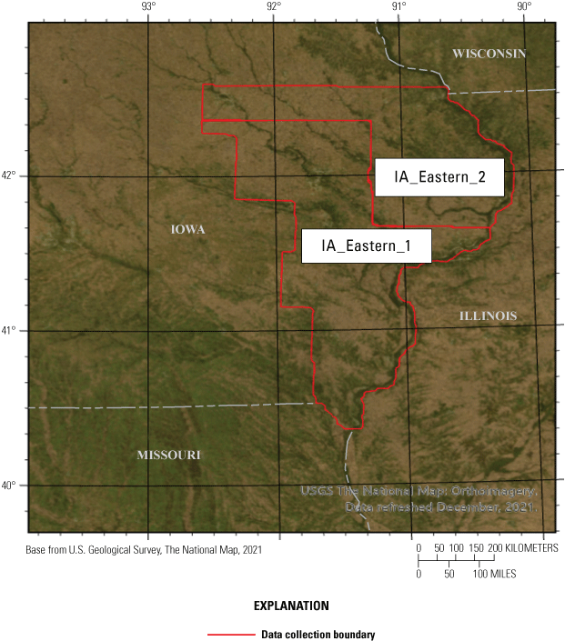
Map showing 3D Elevation Program data collection areas in Iowa referenced in this study.
The sensor specifications used for data collection are listed in table 1. Two interesting characteristics of the sensors are their dual-channel nature and wide area mapping ability because of higher field of view. Although such systems are expected to cover large areas in a shorter amount of time, the increased complexity of the system can require a more elaborate system calibration process (Ravi and Habib, 2020) such as additional cross-channel calibration. There can also be increased point density variation due to wider field of view; therefore, we evaluated the data collected by the sensor to understand its ability to meet the data requirements of 3DEP.
Methods
The methods used for assessing the geometric quality of lidar data vary in terms of the scale (area wise) and the requirements for ground reference data collection. The quality of data for interswath, same-surface precision and point density, and interproject consistency can be measured over the entire spatial extents of the data and do not require ground reference data. Ground reference data using field survey methods are required to determine the absolute accuracy (three dimensional and vertical) of the data. The field survey and the data analysis methods used to characterize and quantify the quality of the lidar data are described in this section.
Ground Reference Data Collection
To test the geometric accuracy of lidar data, a 9-day, one-field survey campaign was planned and designed (Irwin and others, 2024). Field data were collected by the USGS between October 25 and 31, 2020. The locations surveyed in Iowa are shown in figure 2. Real-time kinematic (RTK) Global Navigational Satellite System (GNSS), total station, and ground-based lidar were acquired to compare to the 3DEP data collected. USGS collected these data using survey-grade GNSS and total station instruments along with a terrestrial laser scanner (TLS). For this study, three Trimble R10-2 GNSS antennas (one base and two rovers), a Trimble SX10 robotic total station, and a RIEGL VZ-400i TLS were used. With proper RTK surveying practices, the Trimble R10-2 GNSS antennas can achieve ± 8 millimeters (mm) + 1 ppm horizontal accuracy, and ±15 mm + 1 ppm vertical accuracy relative to the base station. The Trimble SX10 used in this work was a 1-inch instrument with a distance measurement accuracy of ±2 mm + 1.5 ppm. The RIEGL VZ-400i has an accuracy of 5 mm and a precision of 3 mm. In the RTK method, a fixed base station with a known location (base station) transmits corrections to a moving GNSS receiver (rover). The rover uses these corrections to greatly enhance its positional accuracy, achieving centimeter-level precision (Van Sickle, 2008). The base station data were postprocessed through the National Geodetic Survey Online Positioning User Service (OPUS) at least 16 days after collection, when precise ephemeris of the GNSS satellites were available (Soler and others, 2011). OPUS static processing typically provides solutions that are within 1–2 centimeters (cm) horizontally and 2–4 cm vertically within the National Spatial Reference System. The postprocessed base station data were used to update coordinates for the rover points. Those rover points included control points that were established for the total station to occupy and backsight. The ground-based lidar is operated by strategically positioning the lidar scanner to ensure full coverage of the target area. These scans from multiple locations are necessary for complete coverage of most targets due to obstructions. The lidar systematically emits laser pulses and records the return time and intensity of the reflected light, capturing millions of data points. Reflective targets are placed in the region of data collection, and their positions are surveyed using the total station. These targets are used to georeference the lidar data scans and improve the accuracy of merging multiple scans (Bethel and others, 2025). The GNSS and total station data include points collected on ground elevations, infrastructure features, and TLS georeferencing targets. The TLS data include scans of buildings, parking lots, and groups of trees. All survey data were published (Irwin and others, 2024).
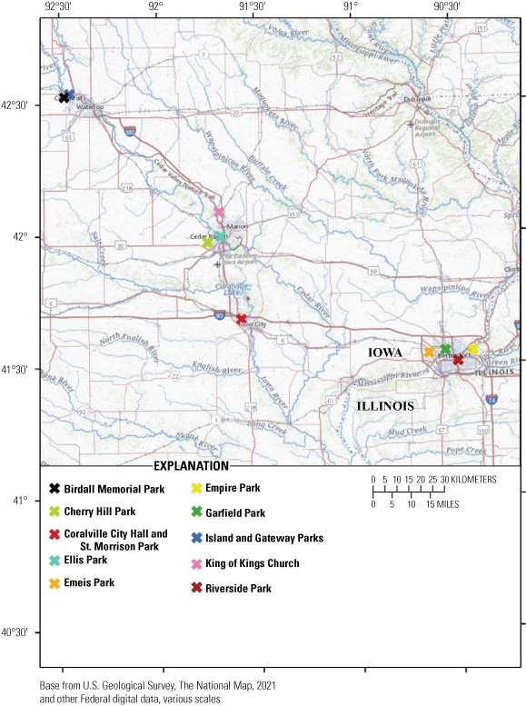
Map showing the location of areas of field data collection in Iowa.
Ground Reference Data Processing
GNSS and total station data were collected using Trimble R10-2 GNSS antennas and a Trimble SX10 robotic total station. The data are processed to be in the Universal Transverse Mercator Zone 15 North projection and are referenced to the North American Datum 1983 National Adjustment of 2011 (epoch 2010) and the North American Vertical Datum 1988 GEOID12B for orthometric heights. Raw GNSS base station data were downloaded from of the base antenna in the manufacturer’s proprietary format. The base files were converted to the Receiver Independent Exchange (RINEX) format using the Convert to RINEX version 3.1.4.0 tool (Trimble Inc.). RINEX files were submitted to OPUS for correction in the National Spatial Reference System. Postprocessed base coordinates, returned from OPUS, were used to update all GNSS RTK points in Trimble Business Center 5.60 (TBC). Updated control point coordinates from the rover were then updated for the total station, thus updating the coordinates of all total station points in TBC. Point shapefiles were exported from TBC.
TLS data were collected with a RIEGL VZ-400i laser scanner. Scan data were downloaded from the scanner and processed using RIEGL’s RiScan Pro 2.14.1 software (http://www.riegl.com/products/software-packages/riscan-pro/). Raw scan data were imported using the download and convert tool. The coordinate reference systems were set via the GeoSysManager. Coarse scan registration was accomplished using the Automatic Registration 2 tool. Fine registration and georeferencing were then determined using the Multi Station Adjustment 2 tool. The point clouds were then colored from images taken by the integrated camera. The scan data were filtered to remove data with a pulse shape deviation of greater than 15. Points with a reflectance of less than −20 decibels were also filtered. Isolated points were removed when less than 5 points were within a 0.300-meter (m) search radius. Finally, all scanner positions were exported as merged files.
Interswath Accuracy Assessment
Interswath accuracy (Stensaas and others, 2018) describes the degree of agreement between overlapping strips of lidar data and measures the horizontal and vertical errors that may exist between conjugate features in the overlapping regions of the data. The errors are estimated by first identifying two overlapping swaths and calculating the distance between a point in one swath and the corresponding best-fit plane in a neighboring patch of points extracted from the overlapping swath. These measurements are aggregated to estimate the relative horizontal and vertical errors between swaths. The interswath accuracy is described in terms of the following metrics:
Same-Surface Precision Assessment
Same-surface precision of the data describes the consistency of the lidar measurements and is measured by extracting points inside a planar surface. Artificial surfaces, such as a flat roof plane or other built-up area, are preferred. Once the lidar points are extracted, a plane is fit to the points and the root mean square error (RMSE) of the planar fit is calculated. Figure 3 shows a synthetic computer-generated data with same-surface precision exaggerated for clarity. Figure 4 shows a real example of a polygon placed over an impervious planar surface.
Graph showing the precision of light detection and ranging point data present inside a polygon over a hard surface. The data are unitless and simulated to show how the precision of lidar data on hard surfaces can be visualized and estimated.
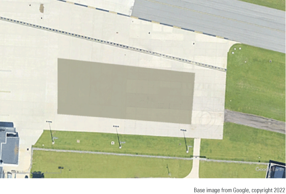
Image showing an example of polygonal area chosen over a hard impervious surface for same-surface precision assessment.
Vertical Accuracy Assessment
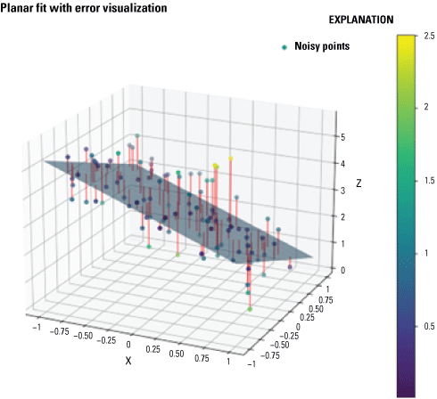
The vertical accuracy of lidar data is measured using checkpoints collected using GNSS or total station survey on flat hard surfaces. 3DEP lidar points within 3 m of the checkpoints are extracted, and a two-dimensional surface is fit to the extracted points. Although a planar fit is normally used, a second order surface more accurately represents local topology (Dey and Wang, 2022); therefore, we decided to use a two-dimensional surface fit z=ax2+bx2+cxy+dx+ey+f. The parameters (a, b, c, d, e, and f) are obtained by extracting the (x, y, z) coordinates of lidar points in the spatial proximity of the checkpoint and fitting the second order equation to the points. The reason for a second order surface fit instead of first order planar fit is that many of these vertical checkpoints have been gathered on road or parking lot surfaces, which can have a mild curvature. The two-dimensional surface fit is used to account for this curvature. If the curvature of the underlying surface is very small, the coefficients of the higher order terms will be estimated as zero or to a very small quantity, which in turn yields the equation of a plane. Figure 5 demonstrates this phenomenon using synthetic computer-generated data and the error shown is exaggerated for clarity.
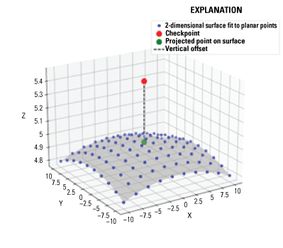
Graph showing vertical accuracy assessment of light detection and ranging data using checkpoints. The data shown are simulated, unitless, and presented to visualize how vertical accuracy is estimated.
At each checkpoint, the error was estimated as follows:
whereÎ
is the error at the check point,
Ζcheckpoint
is the elevation at the check point,
Ζlidar
is the elevation of the lidar data derived using equation 2,
Xcheckpoint
is the x-coordinate of the check point,
Ycheckpoint
is the y coordinate of the check point, and
a, b, c, d, e and f
are the polynomial parameters of the surface.
The vertical error estimates at each checkpoint are combined and reported as RMSE.
Horizontal Accuracy Assessment
The horizontal component of accuracy for 3DEP lidar data is not explicitly verified in most 3DEP projects collected under Geospatial Products and Services Contracts. The Lidar Base Specification (LBS) (USGS, 2024) does not explicitly provide quality thresholds or methods for verification of horizontal accuracy of the data; therefore, the methods presented in this section are forward-looking research efforts to develop operational methods for verifying 3D accuracy (horizontal and vertical) in future versions of the LBS.
In this report, we present three methods to verify the horizontal component of the airborne lidar data accuracy. The first two methods involve using TLS scanned roof planes of houses and other structures and comparing the point cloud data with the 3DEP lidar data. Two methods were used to quantify the comparisons. In the first method, conjugate roof plane points (in TLS and 3DEP lidar data) are manually selected, and the coordinates of the roof are compared (fig. 6). The ellipsoids in figure 6 represent the location uncertainty (due to noise and other factors) for the coordinates determined by TLS and 3DEP lidar data. The TLS derived point (blue ellipsoid) is more precise than the 3DEP derived point (red ellipsoid) due to the higher precision of the TLS data and can be used as control points. This process is described in Kim and others (2020). In the second method, an iterative closest plane algorithm (Chen and Medioni, 1992) is used to determine the offset between TLS point cloud of the roof and the 3DEP point cloud.
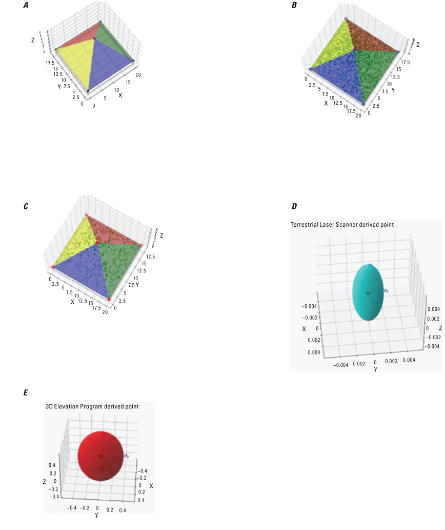
Graphs showing various simulations and unitless data. A, Simulated representation of terrestrial laser scanner (TLS) and aerial light detection and ranging (lidar) data over a roof plane. B, The TLS data are much denser and more precise (less noisy) than the aerial lidar data. C, The coordinates of vertex at the top of the roof plane are determined from the TLS data and 3D Elevation Program (3DEP; https://www.usgs.gov/3d-elevation-program) data mathematically using planar intersection and compared. D, The corresponding uncertainty (due to noise and other factors) for the coordinates of the point are shown. E, The TLS derived point are more precise than 3DEP derived point and can be used as control points.
The third method (fig. 7) for observing horizontal errors in the data used checkpoints collected on visible parking lot or road markings on freshly paved surfaces. In figure 7, the coordinates of blue and the pink dots (surveyed check points) are compared to the manually extracted coordinates of the intersection of the painted lines and the location of the end parking lanes (not shown). This method is used in the industry (Bethel and others, 2006) and is analogous to the data quality assessment methods used for aerial and satellite imagery. Because the LBS do not require horizontal accuracy reported with the 3DEP data delivery, these measurements are usually made by the data vendors for their internal processes and not externally reported.
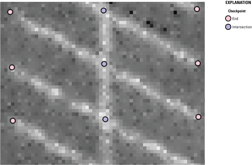
Light detection and ranging intensity image showing parking lot lines and field-surveyed checkpoints in our field data notes (Irwin and others, 2024).
Point Density Assessment
Point density refers to the concentration or frequency of point data within a defined area. In the context of spatial analysis, it represents the number of points per unit area. According to the American Society for Photogrammetry and Remote Sensing’s (ASPRS) recommendations on point density (Bethel and others, 2025), the recommended methodology is a three-step process:
-
· Voronoi polygons (Aurenhammer and Klein, 2000) are generated around each lidar point. These polygons represent the area of influence for that point. Figure 8 represents Voronoi polygons, and point density is estimated as the inverse of the area of each polygon. The number shown within each polygon represents the density (in points per square units) within the polygon.
-
· The density of lidar points is determined by taking the inverse of the area of each Voronoi polygon.
-
· The 5th percentile of the density of points as calculated above is reported.
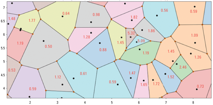
Computer-generated image showing Voronoi polygons and point density for a set of randomly generated points. The data are unitless and the purpose of the visualization is to provide a mental model of the density estimation process.
Interproject Light Detection and Ranging Data Consistency Assessment
The 3DEP is envisaged to support national and panregional scientific and engineering goals; however, many of the lidar acquisition projects (including the current one under study) have scientific goals that are regional or subregional in scope. Their contractual requirements on geometrical data quality are also limited to their spatial extent (Dewberry Inc., 2022b). Lidar data for scientific projects such as river systems analysis, carbon sink assessments, interstate road networks, and watersheds require data assessments that are similar in scope. Many features such as streams, roads, and forests will span multiple and diverse collections or projects, using a varied set of sensors, data processing algorithms, and software. Data may be acquired by different vendors using different sensors at different times; therefore, features must be represented in a consistent manner by the lidar data to ensure accuracy and reproducibility in scientific studies, and the consistency between adjacent datasets must be quantified and documented in the metadata.
The interproject consistency is evaluated by first determining all the relevant projects that the current project under study overlaps. Then, the evaluation follows the same process as the interswath assessment; however, instead of two swaths of the same project being compared, the two overlapping datasets are assessed. Figure 9 demonstrates this process using synthetic points. The two boundaries are determined using alpha shapes and the analysis is performed using the “Intersection Points” in the overlapping region of the alpha shapes.
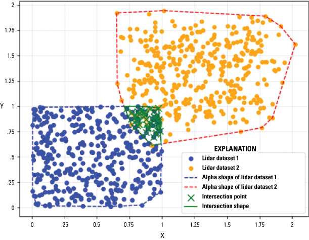
Graph showing randomly generated point datasets of light detection and ranging data from two projects that overlap. The data are unitless and images provide a mental model of how overlapping regions may contain data that can be used to assess their consistency.
Because these are large datasets (for example, the IA_Eastern_1 dataset has 154,630,110,433 points and IA_Eastern_2 has 90,121,793,878 points), this analysis is not trivial. Large computing resources and data handling tactics are needed. Accordingly, this workflow uses lidar data stored in the Entwine Point Tile (EPT; Butler and others, 2021) format on the Amazon Web Services cloud computing platform. The breakdown of the steps involved are as follows:
-
1. Datasets are organized and indexed. The process starts with raw lidar data stored in the EPT format, which is a way to organize and index large point cloud datasets efficiently. The data are in Web Mercator projection (Battersby and others 2014). This makes it easy to compare point cloud data that would otherwise be in different coordinate systems. Care must be taken to ensure that the vertical datum (‘z’ coordinates) is the same.
-
2. Decimated lidar data are read. The Point Data Abstraction Library (PDAL; Butler and others, 2021) is used to read the lidar data from the EPT file. The lidar data are read in a decimated manner, meaning the data are reduced in resolution to a manageable size. The EPT data format has spatial indexing that allows the user to select points at or near a user specified resolution (point spacing). In this example, the point spacing specified was initially 1000 m to read the lidar data for the entire project.
-
3. Boundaries are detected. Once the decimated data are read, the alpha shape (Edelsbrunner and others, 1983) algorithm is used to detect the boundaries of the point cloud. This creates internal and external boundaries, representing the outline of the scanned area and any holes or gaps within it.
-
4. Spatial intersection is determined. Once the external boundaries are identified, the spatial intersection of the two boundaries (an example is shown in fig. 9) is determined. This spatial intersection represents the overlap region of two projects being compared.
-
5. Data are streamed and analyzed. The area of the spatial intersection is usually small compared to the area of projects; therefore, the complete data within the overlap can be streamed and analyzed.
-
6. Steps to analysis are followed. Once the two datasets covering just the overlap region are available, the analysis follows the same steps as the interswath analysis.
Results
The results of the data quality analysis across the parameters described in the previous section are provided in this section. The LBS defines many quality levels for obtaining lidar data (USGS, 2024). The airborne lidar data were collected to satisfy the requirements defined by quality level (QL) 2. A detailed description of the quality levels can be obtained from the LBS, and the relevant information for QL2 is listed in table 2. Although the analysis does not strictly follow the LBS, it is valuable to understand the contracted data quality requirements.
Table 2.
Light detection and ranging (lidar) data requirements from the Lidar Base Specifications for geometric accuracy of quality level 2 lidar data relevant for this report (U.S. Geological Survey, 2024).[QL2, quality level 2; lidar, light detection and ranging; LBS, Lidar Base Specifications; m2, square meter; ≤, less than or equal to; m, meter; <, less than; RMSE, root mean square error; CE 95, circular error at 95th percentile]
The interswath accuracy (as described in Stensaas and others, 2018) was measured for the Iowa lidar dataset by selecting 50 tiles each in a random manner from the project data archive (U.S. Geological Survey, 2022a) for the two Iowa lidar datasets (IA_Eastern_1 and IA_Eastern_2). The accuracy results (tables 3, 4, and 5) indicate that the data are within the specifications. The LBS does not specify horizontal accuracy requirements; however, the methods used here automatically estimate interswath horizontal accuracy also, and the estimates are listed in table 3.
Table 3.
Summary of interswath measurements across 100 tiles in the two datasets of Iowa light detection and ranging data.[AOI, area of interest; RMSD, root mean square difference; m, meter; IA, Iowa]
The same-surface precision of the data was calculated by manually delineating 28 polygons over hard impervious surfaces (using visually inspection) across the two datasets. The data were downloaded from Amazon Web Services (https://registry.opendata.aws/usgs-lidar/) in in the EPT format and evaluated on U.S. Geological Survey provided Amazon Web Services platform. The use of cloud computing platforms and the EPT based format made it easier to evaluate the precision across the project area, because only data that were needed for the analysis were downloaded and used.
Table 4.
Summary of same-surface precision measurements across 28 polygons in the two datasets of Iowa light detection and ranging (lidar) data.[AOI, area of interest; RMSD, root mean square difference; m, meter, IA, Iowa)]
The 3D accuracy (horizontal and vertical accuracy) assessment results are presented in tables 5 and 6. The results based on roof plane intersection and iterative closes plane measurements of buildings scanned using TLS are presented in table 5. The fully automated iterative closest plane method could not be used on two datasets (Island and Gateway Parks 2 and Garfield Park) because of overhanging trees in the 3DEP data. Although there are ways to eliminate lidar points from trees (Sampath and Shan, 2009), those were not used here for simplicity. The summary results using the two methods are very similar and indicate that the two methods lead to consistent results.
Table 5.
Summary of three-dimensional accuracy measurements in the two datasets of Iowa light detection and ranging (lidar) data.[m, meter; NA, not applicable; RMSE, root mean square error]
The horizontal accuracy analysis results based on parking lot markings are presented in table 6. Measurements were made on parking lot marking intersections and end points (fig. 5) at four locations (Garfield Park, Emeis Park, Ellis Park, and Birdall Memorial Park); however, only two locations could be used because the parking lot markings were not visible in the 3DEP lidar intensity data. At Birdall Memorial Park, only the intersections and not the end points were used because the end points were not visible in the intensity raster data. Reference data over Coralville City Hall and St. Morrison Park parking lot were also collected but could not be used because the linear features in the lidar intensity were not clear.
Table 6.
Summary of horizontal accuracy measurements in the two datasets of Iowa light detection and ranging data.[3DEP, 3D Elevation Program; RMSE, root mean square error; m, meter; IA, Iowa].
The vertical accuracy measurements for the two Iowa lidar datasets are reported in table 7. Most of the results are over hard surfaces under clear and open skies. Field data were collected under thick vegetation at the Empire Park location (reported in table 7 as “Empire Park, vegetated”, and a sample of the measurements are shown in fig. 10).
Table 7.
Summary of vertical accuracy measurements in the two datasets of Iowa light detection and ranging (lidar) data.[3DEP, 3D Elevation Program; m, meter; RMSE, root mean square error; IA, Iowa].
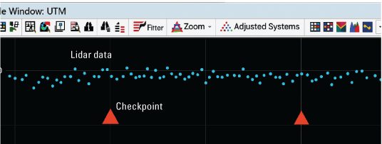
A screen shot (using LP360 2020.2.33.3) showing the profile of light detection and ranging (lidar) data (blue dots) and checkpoints (red triangles) under canopy (vegetated area) (U.S. Geological Survey, 2022b).
The density of the data (results reported in table 8) was measured by randomly selecting 10 tiles of lidar data in the two datasets. The density is reported as the mode value of the measurements. The density estimates were made using Voronoi method (Bethel and others, 2025) at every point in the tiles, and summary statistics were collected.
Table 8.
Summary of point density measurements in the two datasets of Iowa light detection and ranging (lidar) data.[3DEP, 3D Elevation Program; ppsm, points per square meter; IA, Iowa]
Data consistency analysis results performed against adjacent overlapping projects are listed in table 9. The criteria chosen for comparisons were recency in terms of the Iowa lidar data. The recency criteria are important to avoid changes to terrain. The overlap area for these comparisons tends to be very small (fig. 11) in comparison to the area of the projects; therefore, obtaining sufficient valid points (ground classified points in open areas) to perform the analysis is often challenging.
Table 9.
Interproject consistency analysis for the two datasets of Iowa light detection and ranging (lidar) data.[m, meter; RMSD, root mean square deviation; IL, Illinois; vs; versus; IA, Iowa; WI, Wisconsin; USGS, U.S. Geological Survey]
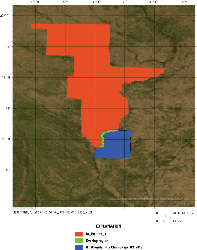
Map showing the overlap of two 3D Elevation Program projects (U.S. Geological Survey, 2022a, 2022c). The interproject consistency measurement region is usually very small, compared to the overall project area.
Discussion
The Iowa lidar data meets or exceeds the expectations for QL2 data in most of the parameters. The complexities of the multichannel and wide-angle nature of the sensor system appear to have been accounted for in the calibration and data quality assurance processes; however, Iowa is a flat region, and the wide-angle sensor systems have not been evaluated in other more topographically challenging conditions.
Interswath and same-surface precision are well within the specified tolerances. Certain tiles exceeded the horizontal accuracy by 0.50 m, but this did not cause error in vertical accuracy because of the relative flatness of Iowa. It should also be noted that although the interswath horizontal accuracy is not required by the LBS, it is an important measure of the quality of calibration because calibration errors manifest more in the horizontal dimensions.
Vertical accuracy on flat areas is excellent, with RMSE values consistently below the 0.10 m threshold for nonvegetated areas. Horizontal accuracy assessments were not explicitly required by the LBS but demonstrate good agreement between lidar and reference data. Point density generally exceeds the minimum requirement of 2 points per square meter. The interproject consistency assessment indicates good agreement between the Iowa lidar data and adjacent datasets and demonstrates that the data quality of the U.S. Geological Survey National Geospatial Program’s 3DEP is sufficient for use in large-scale geospatial projects.
The analysis methods presented here often exceed the data verification requirements outlined in the LBS. Whereas the LBS provides a valuable framework for data quality assessment, the analysis demonstrates that additional metrics and methods can offer a more comprehensive understanding of lidar data quality. For example, the inclusion of horizontal accuracy assessment, although not mandatory in the LBS, provides valuable insights into the data's overall geometric integrity, assuring the users that data quality is uniformly consistent.
Furthermore, the use of cloud computing platforms and efficient data formats like EPT enabled the analysis of massive lidar datasets covering extensive areas. This analysis highlights the potential of modern technologies to streamline and enhance the quality assessment process for large-scale geospatial projects.
The differences between the analysis methods and the LBS specifications also underscore the need for continuous refinement and evolution of data quality standards. As technology advances and new applications for lidar data emerge, it is crucial to adapt and expand the assessment criteria to ensure the data supports the intended applications.
Conclusions
The comprehensive accuracy assessment of the Iowa light detection and ranging (lidar) data demonstrates that 3D Elevation Program data quality is sufficiently reliable for use in large-scale geospatial projects and analyses. The data meets or exceeds the specifications for quality level 2 data outlined in the Lidar Base Specifications, with excellent interswath and same-surface precision (<0.10 m), high vertical and horizontal accuracy, sufficient point density, and good consistency with adjacent datasets. The Iowa lidar data can be used for several applications, such as flood plain mapping, land use planning, infrastructure management, and scientific research.
This assessment also highlights how going beyond the minimum data quality requirements specified in the Lidar Base Specifications can help gain a deeper understanding of lidar data quality. The use of Additional metrics and methods like those used in this study can be used by data producers and users to gain additional insights into the geometric integrity of large-scale datasets.
We did not assess data quality under canopy in this study, but future lidar data collection projects could incorporate assessments of data quality under canopy to further improve the quality of lidar data. Point density and classification accuracy are major parameters used for data validation. The methodologies presented in this report could be used to inform the continuous refinement and evolution of lidar data quality standards to keep pace with technological advancements and the evolving needs of lidar data users.
References Cited
Bethel, M., Abdullah, Q., Damkjer, K., Nimetz, J., Sampath, A., Newcomb, D., Chambers, B., Butler, H., Damkjer, K., Mcgaughey, R., Miller, B., Janiec-Grygo, M., Penton, J., Karlin, A., Eick, N., Greblowska, D., 2025, ASPRS guidelines on quantifying horizontal sampling density of aerial lidar point cloud data (1st ed., ver. 1.0): American Society for Photogrammetry and Remote Sensing, 27 p., accessed April 24, 2025, at https://publicdocuments.asprs.org/LidarDensity-Ed1-V1.
Dewberry Engineers Inc., 2022a, IA_Eastern_2019-WUID, 300007: U.S. Geological Survey contractor report, 34 p., accessed May 20, 2024, at https://prd-tnm.s3.amazonaws.com/StagedProducts/Elevation/metadata/IA_EasternIA_2019_B19/IA_Eastern_2_2019/reports/IA_Eastern_WUID300007_Report.pdf.
Dewberry Engineers Inc., 2022b, 3D Nation elevation requirements and benefits study—Final report: Silver Springs, Md., National Oceanic and Atmospheric Administration, prepared by Dewberry Engineers Inc., Fairfax, Va., 171 p., accessed May 20, 2025, at https://iocm.noaa.gov/reports/3dnationstudy/3D_Nation_Study_Final_Report.pdf.
Edelsbrunner, H., Kirkpatrick, D.G., and Seidel, R., 1983, On the shape of a set of points in the plane: IEEE Transactions on Information Theory, v. 29, no. 4, p. 551–559, r12, accessed December 12, 2024, at https://doi.org/10.1109/TIT.1983.1056714.
Irwin, J.R., Danielson, J.J., Robbins, T.J., Kropuenske, T.J., Sampath, A., Kim, M., and Park, S., 2024, 2019 Eastern Iowa topographic lidar validation—USGS field survey data: U.S. Geological Survey data release, accessed December 12, 2024, at https://doi.org/10.5066/P9DI0G64.
Kim, M., Park, S., Irwin, J., McCormick, C., Danielson, J., Stensaas, G., Sampath, A., Bauer, M., and Burgess, M., 2020, Positional Accuracy Assessment of Lidar Point Cloud from NAIP/3DEP Pilot Project: Remote Sensing (Basel), v. 12, no. 12, p. [Also available at https://doi.org/10.3390/rs12121974.]
Ravi, R., and Habib, A., 2020, Fully automated profile-based calibration strategy for airborne and terrestrial mobile LiDAR systems with spinning multi-beam laser units: Remote Sensing (Basel), v. 12, no. 3, p. 401, accessed December 12, 2024, at https://doi.org/10.3390/rs12030401.
U.S. Geological Survey, 2022a, Index of/ vdelivery/ datasets/ staged/ elevation/ LPC/ projects/ IA_easternIA_2019_B19/IA_eastern_1_2019/: U.S. Geological Survey website, accessed May 22, 2024, at https://rockyweb.usgs.gov/vdelivery/Datasets/Staged/Elevation/LPC/Projects/IA_EasternIA_2019_B19/IA_Eastern_1_2019/.
U.S. Geological Survey, 2022b, USGS lidar point cloud IA_easternIA_2019_B19 15TXG110550: U.S. Geological Survey dataset, accessed May 22, 2024, at https://www.sciencebase.gov/catalog/item/6359c4cdd34ebe442503f0ab.
U.S. Geological Survey, 2022c, USGS lidar point cloud IL_8county_pluschampaign_B2_2019: U.S. Geological Survey dataset, accessed May 22, 2024, at https://stac.geoplatform.gov/external/s3-us-west-2.amazonaws.com/usgs-lidar-stac/ept/IL_8County_PlusChampaign_B2_2019.json?.language=en.
U.S. Geological Survey, 2024, Lidar base specification online (rev. A): U.S. Geological Survey, accessed May 15, 2025, at https://www.usgs.gov/ngp-standards-and-specifications/lidar-base-specification-online.
Conversion Factors
Datums
Vertical coordinate information is referenced to the North American Vertical Datum of 1988 (NAVD 88).
Horizontal coordinate information is referenced to the North American Datum of 1983 (NAD 83).
Abbreviations
3D
three-dimensional
3DEP
3D Elevation Program
EPT
Entwine Point Tile
GNSS
Global Navigation Satellite System
LBS
Lidar Base Specifications
Lidar
light detection and ranging
OPUS
Online Positioning User Service
PDAL
Point Data Abstraction Library
ppm
points per million
ppsm
points per square meter
QL
quality level
RINEX
Receiver Independent Exchange
RMSE
root mean square error
RMSD
root mean square deviation
RTK
real-time kinematic
TBC
Trimble Business Center
TLS
terrestrial laser scanner
For more information about this publication, contact:
Director, USGS Earth Resources Observation and Science Center
47914 252nd Street
Sioux Falls, SD 57198
605–594–6151
For additional information, visit: https://www.usgs.gov/centers/eros
Publishing support provided by the
Rolla and Lafayette Publishing Service Centers
Disclaimers
Any use of trade, firm, or product names is for descriptive purposes only and does not imply endorsement by the U.S. Government.
Although this information product, for the most part, is in the public domain, it also may contain copyrighted materials as noted in the text. Permission to reproduce copyrighted items must be secured from the copyright owner.
Suggested Citation
Sampath, A., Irwin, J., and Kropuenske, T., 2025, Validation of the geometric accuracy of airborne light detection and ranging data for eastern Iowa, 2019: U.S. Geological Survey Open-File Report 2025–1017, 16 p., https://doi.org/10.3133/ofr20251017.
ISSN: 2331-1258 (online)
Study Area
| Publication type | Report |
|---|---|
| Publication Subtype | USGS Numbered Series |
| Title | Validation of the geometric accuracy of airborne light detection and ranging data for eastern Iowa, 2019 |
| Series title | Open-File Report |
| Series number | 2025-1017 |
| DOI | 10.3133/ofr20251017 |
| Publication Date | June 02, 2025 |
| Year Published | 2025 |
| Language | English |
| Publisher | U.S. Geological Survey |
| Publisher location | Reston, VA |
| Contributing office(s) | Earth Resources Observation and Science (EROS) Center |
| Description | Report: v, 16 p.; Data Release |
| Country | United States |
| State | Iowa |
| Online Only (Y/N) | Y |
| Additional Online Files (Y/N) | N |