

Gillnet Sampling Methods for Monitoring Status and Trends of Clear Lake Hitch in Clear Lake, Lake County, California
Links
- Document: Report (2.5 MB pdf) , HTML , XML
- Data Release: USGS data release - Abundance and distribution of fishes in Clear Lake, Lake County, California
- Download citation as: RIS | Dublin Core
Acknowledgments
Funding was provided by the U.S. Fish and Wildlife Service via Inter-Agency Agreements 4500100031, 4500109755, 4500113034, and 4500146328. The support of Elisha Hull and Amber Aguilera of the U.S. Fish and Wildlife Service made this work possible. Additional funding was provided by the U.S. Geological Survey (USGS), Southwest Region and California Water Science Center. Clear Lake Hitch sampling was authorized by scientific collection permits and associated memorandums of understanding issued by the California Department of Fish and Wildlife. Dave Ayers, Ethan Clark, Anna Conlen, Ethan Enos, Marry Jade Farruggia, Bret Fessenden, Emerson Gusto, Jessie Kathan, Anthony Martinez, Oliver Patton, Dennis Valentine, Mitch Zheng, and numerous other individuals assisted on the project. Robinson Rancheria’s Fisheries Program was able to contribute and partner with USGS thanks to the U.S. Fish and Wildlife’s Tribal Wildlife Grant Program and the Yocha Dehe Giving Fund. The following Tribes also provided substantial support to the project: Habematolel Pomo of Upper Lake, Big Valley Rancheria, and Elem Indian Colony.
Abstract
The Clear Lake Hitch (Lavinia exilicauda chi) is a minnow endemic to Clear Lake, Lake County, California. This species is listed as a threatened species under the California Endangered Species Act and has been petitioned for listing under the United States Endangered Species Act. In 2017, the U.S. Geological Survey, in cooperation with the U.S. Fish and Wildlife Service, initiated a Clear Lake Hitch monitoring program to generate information annually on relative abundance and size structure. The monitoring program was organized around a conceptual life cycle diagram, focused on life stages approximately ≥1 year of age, and incorporated a probabilistic study design involving approximately 10 days of short-duration (approximately 40 minutes) gillnet sampling undertaken during daytime. This report documents monitoring program activities from 2017 to 2023 and presents the results of an evaluation of the monitoring program. The evaluation was done after the 2023 sampling event, following 6 years of implementation, which is the approximate generation cycle of Clear Lake Hitch. The results of the evaluation indicated the following: (1) gillnets used in the monitoring program were effective at capturing Clear Lake Hitch aged 1 year or more; (2) the study design was effective at generating the information needed to characterize Clear Lake Hitch relative abundance and size structure, and meaningful operational efficiencies can be obtained by implementing simple changes; and (3) future sampling can be scaled to approximately 4–7 days of effort and maintain at least 80-percent confidence in detecting at least a 25-percent change in abundance, assuming past work productivity is maintained and future data are typical of previous data.
Introduction
The Clear Lake Hitch (Lavinia exilicauda chi) is a minnow endemic to Clear Lake, Lake County, California, that is listed as threatened under the California Endangered Species Act; it also has been petitioned for listing under the United States Endangered Species Act (fig. 1). Management interest in Clear Lake Hitch originates, in part, from historical accounts that suggest it was formerly highly abundant and an important resource for Native American Tribes (Moyle, 2002; California Department of Fish and Wildlife [CDFW], 2014). A variety of factors are thought to have synergistically contributed to a substantial contemporary decline in Clear Lake Hitch abundance. These factors include the loss and degradation of stream habitat used for spawning and rearing caused by changes in land and water use in the watershed and the loss and degradation of lacustrine habitat caused by shoreline development, reclamation of wetlands, and broad-scale changes to biological and physio-chemical components of Clear Lake (Moyle, 2002; California Department of Fish and Wildlife, 2014).

Adult Clear Lake Hitch collected from Clear Lake, Lake County, California.
Effective conservation and management of Clear Lake Hitch requires basic information on the population’s status and trends. In an attempt to address this need, in 2017, the U.S. Geological Survey, in cooperation with the U.S. Fish and Wildlife Service, initiated a Clear Lake Hitch monitoring program. Active Tribal participation implementing the monitoring program began in 2022. The monitoring program has consisted of sampling the Clear Lake Hitch population within Clear Lake with gillnets to generate information annually on population abundance and size structure. This report describes monitoring program activities from 2017 to 2023 and presents the results of an evaluation of monitoring program activities after 6 years of implementation, which is the approximate generation cycle of Clear Lake Hitch. The evaluation sought to (1) assess the effectiveness of the monitoring program in generating the desired information on population abundance and size structure and (2) estimate the amount of sampling effort needed annually in the future to successfully detect real trends in Clear Lake Hitch abundance.
Study Area
Clear Lake is in central California, approximately 100 kilometers (km) north of San Francisco Bay (fig. 2). It is at 400 meters (m) elevation within the central California foothills and coastal mountains ecoregion of California, which is characterized by low mountain foothills with chaparral and oak woodlands (Griffith and others, 2016). With a surface area of 17,700 hectares (ha) and a volume of 1.4 billion cubic meters (m3), Clear Lake is the largest natural freshwater lake within California and the 33rd largest in the conterminous United States (Bue, 1963). The contemporary climate is Mediterranean with hot, dry summers and cool, moist winters. Clear Lake is fed by numerous intermittent streams that deliver freshwater seasonally in winter and spring from a 110,000 ha watershed. Clear Lake has one outlet, Cache Creek, which drains out of the southern-most point of Clear Lake and runs approximately 100 km before connecting to the Sacramento–San Joaquin Delta.

Clear Lake, Lake County, California, showing the 1,529 sites where gillnets were deployed during Clear Lake Hitch sampling from 2017 to 2023. The Clear Lake outline was obtained from the State of California’s California Lakes dataset (California Department of Fish and Wildlife, 2024). The depth layer was interpolated from 1,529 discrete depth measurements associated with each gillnet deployment, summarized from Palm and others (2023). Inset map shows the location of Clear Lake within California.
Clear Lake Hitch Life Cycle
Clear Lake Hitch has a complex potamodromous life cycle in which it occupies a diversity of habitats across the landscape (fig. 3; Murphy, 1948; Moyle, 2002). Reproduction occurs during spring when adult Clear Lake Hitches migrate from Clear Lake into tributary streams to spawn. The tributary streams are ephemeral and typically only flow during winter and spring in response to heavy seasonal rain. Therefore, all aspects of reproduction, including adult migration, spawning, embryo incubation, larval development, and emigration, must occur during a relatively short temporal window when streamflow and water temperature are suitable (Feyrer, 2019). Numerous streams in the watershed are used for spawning, but it is not known if individuals return to their natal habitats to spawn (Feyrer and others, 2019a). Offspring appear to spend about 40 days on average in natal streams before moving to Clear Lake (Feyrer and others, 2019a). Individuals will live the remainder of their lives in Clear Lake, aside from presumably annual spawning migrations into streams upon reaching sexual maturity at approximately 2 years of age and a size of about 175 millimeters (mm; Geary and Moyle, 1980; Moyle, 2002); Clear Lake Hitch is thought to be iteroparous based upon the absence of dead adults on spawning grounds. Some spawning has been observed along the shoreline of Clear Lake (Kimsey, 1960), but the relative contribution of stream versus lake production of juvenile fish to the population is unknown. Clear Lake Hitches occupy a diversity of habitats within Clear Lake, with juveniles associated with nearshore littoral zones and adults mostly associated with offshore pelagic zones (Murphy, 1948; Moyle, 2002; Young and others, 2022). Clear Lake Hitches reach approximately 6 years of age and attain a maximum size of at least 385 mm standard length (SL; Geary and Moyle, 1980; Palm and others, 2023).

Generalized conceptual life cycle diagram of Clear Lake Hitch and life stages sampled by the gillnet survey in Clear Lake, Lake County, California. The boxes highlight life stages of Clear Lake Hitch aged 2 years or more (age–2+ years) that are sexually mature. The curly bracket highlights life stages for Clear Lake Hitch aged 1 year or more (age–1+ years) sampled by the gillnet survey.
Methods
Clear Lake Hitch Monitoring, 2017–23
The fundamental objective of the Clear Lake Hitch monitoring program was to generate data annually on population abundance and size structure. The monitoring program was organized around a conceptual life cycle diagram of the Clear Lake Hitch and focused on fish approximately aged 1 year or more (fig. 3). The focus on age-1 and older life stages originated from a need to collect as much data as possible on the population with limited resources. It was determined that the best use of available resources was to implement a gillnet survey to be undertaken annually within Clear Lake because it could generate data for all but the age-0 life stage (fig. 3). Although this choice provided a strong return on investment, it also resulted in a notable absence of data on Clear Lake Hitch in the first year of life (age-0 life stage), which could limit inferences concerning factors driving juvenile recruitment.
The Clear Lake Hitch population was sampled with gillnets annually from 2017 to 2023 (fig. 4); however, no work was done in 2020 because of the coronavirus disease (COVID-19) pandemic (fig. 5). Sampling involved once-per-year events in early summer (late June into early July). Early summer was selected for two key reasons. First, it is a non-breeding season when Clear Lake Hitch distribution is constrained within Clear Lake because streamflow in the watershed is low and unsuitable to support spawning (as indexed in fig. 6 by Kelsey Creek), so the entire population is available for sampling. Second, water temperatures are relatively cool compared to later in the summer in July and August, minimizing fish stress and mortality (fig. 6). Sampling effort involved approximately 10 days of work each year. This level of effort originated from an initial goal of estimating population size via a mark-recapture approach. In the study’s first year, 2017, one week of effort (5 days) was dedicated to capturing and tagging fish, and a second week of effort was dedicated to recapturing tagged fish. An inability to recapture tagged fish contributed to an immediate shift in focus to sampling for the purposes of generating interannual indices of abundance. Although abundance indices do not provide data on actual population size, they are usually proportional to population size and are a common and effective metric for monitoring and managing fish populations (Maunder and Punt, 2004; Říha and others, 2023).

A, Gillnet sampling in Clear Lake, Lake County, California, and B, processing of Clear Lake Hitch sampled from Clear Lake.

Key events during the Clear Lake Hitch gillnet survey in Clear Lake, Lake County, California.

A, Seasonal water surface temperature (°C) of Clear Lake, Lake County, California, 2019–22. Data were obtained from the University of California, Davis (UCD, 2024; Lake Monitoring site = UA-06; Longitude: −122.8170, Latitude: 39.0610). The box represents the median and interquartile range (IQR), and the whiskers extend to 1.5 times the IQR. B, Flow in cubic meters per second (m3/s−1) in Kelsey Creek, a major tributary to Clear Lake, during the study period. Data were obtained from U.S. Geological Survey, site 11449500 (U.S. Geological Survey, 2024). Vertical gray bars indicate periods when fish sampling was done.
Sampling was undertaken via short-duration (approximately 40-minute) sets of experimental, multi-mesh monofilament gillnets during daytime. Short duration gillnet deployments were done to minimize stress and mortality of entangled fishes. Gillnets were selected as the most appropriate sampling tool because of considerations regarding Clear Lake Hitch behavior and the physical habitat of Clear Lake. First, Clear Lake Hitch are relatively large, fast-swimming fish that are thought to occupy the full extent of available lacustrine habitat vertically (surface to bottom) and laterally (shallow to deep) when water quality conditions are suitable (Myrick and Cech, 2000; Moyle, 2002; Feyrer and others, 2019b). Second, Clear Lake has a diversity of littoral and demersal physical habitat types consisting of combinations of rock formations of varying size, sand, mud, and emergent and submerged vegetation. Thus, gillnets were considered to be the only sampling tool that could provide a consistent, standardized approach for sampling in all possible lacustrine habitats for age-1+ Clear Lake Hitch. Other sampling tools, such as beach seines, various towed nets, or boat electrofishing, could potentially be effective in only a subset of the total available habitat for specific life stages.
The gillnets used in the study were similar to the American Fisheries Society’s proposed standardized gillnet (Bonar and others, 2009; Hubert and others, 2012), with modifications based on our previous experience sampling Central Valley Hitch (Lavinia exilicauda) and other native minnows in the nearby Sacramento–San Joaquin Delta (Nobriga and others, 2005; Feyrer and others, 2015; Wulff and others, 2022). The gillnets measured 45.7 m in length, with five equal-length panels of 38 mm, 51 mm, 64 mm, 76 mm, and 89 mm stretch mesh. Gillnets deployed on or near the lake bottom were 1.8 m in height, whereas gillnets deployed suspended below the surface were 3.6 m in height.
The core study design involved probabilistic sampling stratified to distribute effort (number of gillnet deployments) proportionally to the surface area of the three geographic arms of Clear Lake: upper, middle, and lower (fig. 2). Random sampling sites were generated and were located in the field. In most instances, two (minimum = one, maximum = eight) gillnets were deployed at each random site, one at the surface and one at the bottom. Orientation of gillnets to shore was not standardized and varied based upon prevailing habitat and weather conditions. Individual gillnet deployments associated with a single random site were set at least approximately 300 m apart from each other in an attempt to ensure that each deployment represented a single independent sample.
Two notable adjustments to the core study design were implemented in 2021 and continued through 2023 (fig. 5). First, in response to a habitat modeling exercise (Feyrer and others, 2019b), deployment of bottom gillnets was terminated at sites that were deemed hypoxic (in other words, the bottom dissolved oxygen concentration was <2.0 milligrams per liter [mg/L]). In place of the bottom gillnet deployments, gillnets were deployed suspended above the bottom hypoxic zone at a depth corresponding to approximately where dissolved oxygen concentration was ≥2.0 mg/L. Second, an adaptive cluster sampling (ACS) component was added in attempt to increase the number of Clear Lake Hitch observations (Thompson, 1990; Turk and Borkowski, 2005). Justification for the ACS component was twofold. First, counts of Clear Lake Hitch in samples were extremely zero inflated (fig. 7), and additional observations could potentially improve the ability for modeling factors such as distribution and habitat associations. Second, overall population abundance of Clear Lake Hitch had declined substantially, and additional fish captures were sought in an attempt to maintain the ability to accurately characterize the size structure of the population. Operational rules for the ACS design involved conducting up to two additional rounds of gillnet deployments at a site within 500 m of the location of the Clear Lake Hitch capture. Specifically, if at least one Clear Lake Hitch was encountered in a deployment, then a subsequent deployment was done, up to a total of three possible sets of deployments.

Counts of adult Clear Lake Hitch aged 2 years or more (age-2+; ≥175 millimeters [mm] standard length [SL]) and juvenile Clear Lake Hitch aged 1 year or more (age-1+; <175 mm SL) in gillnet deployments in Clear Lake, Lake County, California. Data summarized from Palm and others (2023).
Weight in grams (g) and SL in mm were measured and recorded for each individual Clear Lake Hitch captured. Additionally, each individual Clear Lake Hitch captured from 2017 to 2022 was implanted with a passive integrated transponder (PIT) tag. PIT tagging was implemented with the goal of using data from recaptured tagged fish to calculate mark-recapture population estimates (originally in 2017, as described above) and to build information on fish growth and movements. However, no tagged fish (N=547) were ever recaptured, and tagging was terminated in 2023. Delayed mortality is one plausible explanation for the absence of recaptured tagged fish. However, delayed mortality is an unlikely explanation for two reasons. First, identical sampling and tagging methods generated recaptures of Central Valley Hitch in another study done in the Sacramento–San Joaquin Delta (Steinke and others, 2019). Second, identical sampling and tagging methods were able to document long distance and long duration migrations of Sacramento Pikeminnow (Ptychocheilus grandis), a different species but a native minnow of generally similar size and morphology to Clear Lake Hitch (Valentine and others, 2020). Individual Clear Lake Hitch were classified as either juveniles (sexually immature SL <175 mm) or adults (sexually mature aged 2 years or more; SL ≥175 mm) based on information from Geary and Moyle (1980). After processing, all Clear Lake Hitch were released alive at the site of capture, except for a small subset of individuals that were randomly retained each year for a variety of life history studies (Feyrer and others, 2019a; Young and others, 2022). Species identifications and lengths were also recorded for all other fishes encountered (Palm and others, 2023).
Ancillary data recorded for each individual gillnet deployment included the following: date, start time, end time, water depth (three separate measurements, one at the horizontal midpoint and one at each end of a deployed gillnet), gillnet depth (depth at the vertical midpoint of the net), geographic coordinates, gillnet mesh size in which an individual fish was captured, weather variables, and water quality variables. Weather variables included categorical representations of wind speed, wind direction, and precipitation. The following water quality variables were measured with handheld YSI EXO2 sondes (Yellow Springs Instruments, Yellow Springs, Ohio): temperature in degrees Celsius (°C), dissolved oxygen concentration (mg/L), specific conductance in microsiemens per centimeter (µS/cm at 25 °C), turbidity in Formazin Nephelometric Units (FNU), chlorophyll a (a green pigment that absorbs light energy and is a key component of photosynthesis) concentration in micrograms per liter (µg/L), and pH. Two different sets of water quality measurements were recorded: (1) discrete measurements associated with the exact position of each individual gillnet and (2) a single continuous vertical profile associated with each random site. Further data description can be found in the metadata for the published dataset (Palm and others, 2023).
Data collection and management protocols were guided by the U.S. Geological Survey’s Fundamental Science Practices, which clarify how science is done and how the resulting data products are developed, reviewed, approved, and released. For this project, specific data workflow steps included electronic field data entry via laptop computers, automated and manual field data checks, daily database backup, post-survey quality assurance and quality control protocols, agency data review and approval, and data publication. Interested readers who wish to learn more about U.S. Geological Survey Fundamental Science Practices and data management are encouraged to visit USGS (2025a) and USGS (2025b), respectively.
Clear Lake Hitch Monitoring Evaluation
Reynolds and others (2016) characterize critical monitoring program evaluation as a “learn and revise” phase of the typical monitoring program life cycle. It is an essential step to ensure program objectives are being met and to make certain that the data and information being generated meet the needs of resources managers and stakeholders. This evaluation of the Clear Lake Hitch monitoring program was initiated after the program had been implemented for approximately one full Clear Lake Hitch generation (6 years) and centered around three fundamental issues posed here as basic study questions:
-
(1) Has the sampling gear been effective at capturing Clear Lake Hitch?
-
(2) Has the study design been effective at generating the information needed to characterize Clear Lake Hitch population abundance and size structure?
-
(3) What level of sampling effort is needed moving forward?
These three basic study questions involved several specific technical elements. Question 1 focused on quantifying the retention selectivity of the gillnets to determine if the gillnets generated an accurate representation of age-1+ Clear Lake Hitch. Question 2 focused on assessing the core study design and various nuances for calculating a standardized index of abundance and assessing length-frequency distribution. Question 3 focused on a power analysis to guide the level of effort that should be undertaken in future years.
Gillnet Retention Selectivity
Size-selectivity retention curves were developed for each gillnet mesh size similar to Wulff and others (2022). The curves were fit via normal with common spread models implemented following the methods described in the “gillnetfunctions” code for the R statistical programming language (Millar and Holst, 1997). The models were constructed using SL classes set in 10-mm increments and under the context that each mesh size had equal sampling effort. Results were evaluated by assessing deviance values and visually inspecting the selectivity curves and residuals. In addition to the deviance values, patterns in the residuals also provide an indication of how well a model fits data. Negative residuals indicate fewer fish caught than the model expected, whereas positive residuals indicate more fish were caught than expected (Millar and Holst, 1997). In this analysis, small and randomly distributed residuals would indicate good fit, whereas large or systematically patterned residuals could potentially indicate poor fit.
Standardized Abundance Index
The objective of this element was to standardize an approach for calculating annual indices of abundance for juvenile and adult Clear Lake Hitch. Standardization allows abundance indices to be more reliably compared among years, thereby providing meaningful data to evaluate status and trends over time (Bonar and Hubert, 2002; Radinger and others, 2019). This exercise involved assessing a variety of sampling nuances and an evaluation of three candidate standardized abundance indices. The sampling nuances that were evaluated included an assessment of the aforementioned changes that were implemented from 2021 to 2023 (gillnet placement in response to dissolved oxygen concentration and ACS), surface versus mid-depth suspended gillnet deployment on fish counts, and time of day on fish counts.
The effect of dissolved oxygen concentration on counts of juvenile and adult Clear Lake Hitch in gillnet deployments was tested to determine if terminating gillnet deployments in hypoxic (dissolved oxygen concentration <2.0 mg/L) water quality conditions starting in 2021 was warranted and if it should be continued. Dissolved oxygen concentration was previously shown to have a significant effect on fish counts during 2017–18 (Feyrer and others, 2019b) but is re-examined here with an additional year (2019) of data and a different modeling scheme. The effect of dissolved oxygen concentration on counts of juvenile and adult Clear Lake Hitch in gillnet deployments was tested via a generalized linear mixed model (GLMM). The analysis was limited to data collected during 2017–19 because that was the period when sampling was done irrespective of dissolved oxygen conditions. The response variable in the GLMM was the count of either juvenile or adult Clear Lake Hitch in a gillnet deployment. The effect of dissolved oxygen concentration on counts was assessed in the GLMM as a categorical variable with two levels, hypoxic (dissolved oxygen concentration <2.0 mg/L) and normoxic (dissolved oxygen concentration ≥2.0 mg/L). The GLMM included gillnet deployment time (log[minutes]) as an offset to account for sampling effort and included year and region as random effects to account for spatio-temporal dependencies. An object-level random effect (OLRE) was also included to account for zero inflation (Harrison, 2014). The GLMM was fit with a Poisson distribution using the package “lme4” in the R statistical computing environment (Bates and others, 2015; R Core Team, 2020).
The comparison of surface versus mid-depth suspended gillnet deployments was done to determine if the two deployment schemes generated redundant information. Addressing this issue could potentially contribute to improved field operational efficiency because deploying mid-depth suspended gillnets requires substantially more effort than surface gillnets. If the two deployment schemes generated redundant information, logistical efficiencies could be obtained in future years by terminating suspended deployments. The effect of surface versus mid-depth suspended gillnet deployments on counts of juvenile and adult Clear Lake Hitch was tested via a GLMM. The analysis involved data collected during 2021–23, the period when both surface and mid-depth suspended gillnet deployments were completed. The response variable in the GLMM was the count of either juvenile or adult Clear Lake Hitch. The effect of deployment scheme on counts was assessed in the GLMM as a categorical variable with two levels: mid-depth suspended and surface. The GLMM included gillnet deployment time (log[minutes]) as an offset to account for sampling effort. Unlike the previous GLMM constructed to test the effect of dissolved oxygen concentration, this GLMM did not include year, region, or object as random effects because of sparse data (for example, three total instances of positive counts for juvenile Clear Lake Hitch and 28 instances of positive counts for adult Clear Lake Hitch). Instead, site was included as a random effect to account for instances when surface and suspended deployments were paired at a single site. The GLMM was fit with a Poisson distribution using the package “lme4” in the R statistical computing environment (Bates and others, 2015).
The effect of time of day on counts of juvenile and adult Clear Lake Hitch in gillnet deployments was examined because future sampling effort could potentially be undertaken at specific times of day when it would be most effective and improve operational efficiencies in the field. Sampling was done from the early morning crepuscular period through midafternoon because of logistical and safety considerations. There are two key reasons why fish counts could possibly have varied across this time period. First, activity patterns of many fish species vary diurnally and any such behavior by Clear Lake Hitch could have affected their vulnerability to a passive sampling method, such as the gillnets. Second, diurnal variability in light intensity could potentially contribute to systematic patterns of visual avoidance of the gillnets. The effect of time of day on counts of juvenile and adult Clear Lake Hitch was tested via a GLMM using all sampling data. The response variable in the GLMM was the count of either juvenile or adult Clear Lake Hitch in a gillnet deployment. The effect of time of day was included in the GLMM as a fixed effect as hour of day and coded as an integer so that the model calculated a slope across hours. For example, all samples collected during the 05:00 hour were coded 5, all samples collected during the 06:00 hour were coded 6, and so on. The GLMM included gillnet deployment time (log[minutes]) as an offset to account for sampling effort and included year and region as random effects to account for spatio-temporal dependencies. An OLRE was also included to account for zero inflation (Harrison, 2014). The GLMM was fit with a Poisson distribution using the package “lme4” in the R statistical computing environment (Bates and others, 2015).
Three separate candidate standardized abundance indices were developed: (1) nominal, (2) normoxic, and (3) normoxic without ACS. The nominal index was calculated from all sample data. The normoxic index was calculated from all sample data but excluded samples with hypoxia (dissolved oxygen concentration <2.0 mg/L). The normoxic without ACS index was calculated from the latter sample data but excluded the additional effort undertaken with ACS. Annual abundance indices were calculated as the mean number of either juvenile or adult Clear Lake Hitch captured per 60 minutes of standardized gillnet deployment time. Ninety-five percent confidence intervals were calculated to estimate an associated margin of error. A confidence interval conveys the probability that a parameter of interest falls between a pair of values around the mean. The appropriate interpretation of a 95-percent confidence interval here, in the context of an abundance index calculated as a mean value, is that if any given annual survey was replicated 100 times, the upper and lower 95-percent confidence intervals represent the range of values that the abundance index would be expected to fall between in 95 of the 100 replicated surveys.
Length-Frequency Distribution
Length-frequency distribution was the metric used to assess Clear Lake population size structure. Annual data on length-frequency distribution provided a snapshot of the relative proportions of specific size (and by extension, age) groups of individuals that comprise the population. This type of data provides important information about the dynamics of the Clear Lake Hitch population, such as patterns of year-class strength, growth, and mortality (Neumann and Allen, 2007). Annual length-frequency distributions were constructed and compared for the same three scenarios considered for the candidate standardized abundance indices: (1) nominal, (2) normoxic, and (3) normoxic without ACS.
Power Analysis to Guide Future Effort
Power analysis is an important tool to plan ecological studies because, among many things, it can guide the collection of sufficient data to facilitate reliable inferences about population trends over time (Maxwell and Jennings, 2005; Wagner and others, 2013). Statistical power represents the probability to correctly detect a real effect when one exists and depends on sample size, effect size, and the decision criterion (Gerrodette, 1987; Wagner and others, 2013). Consider that a linear model constructed to test if Clear Lake Hitch abundance has increased or decreased over time has a null hypothesis (H0) of no change in abundance over time and an alternative hypothesis (H1) of a change (positive or negative) in abundance over time. Failing to reject the null hypothesis when it is false (falsely concluding there is no change in Clear Lake Hitch abundance over time) would be what is commonly referred to as a Type II error (β). Statistical power is a value that represents the probability of successfully rejecting the null hypothesis when it is false (1-β). Thus, in the context of this analysis, power represents the probability of successfully detecting a real trend in Clear Lake Hitch abundance over time. A power value of 0.80 (80-percent probability of detecting a real trend) is a conventional value typically deemed good for fish monitoring programs (Wagner and others, 2013).
The objective of the power analysis was to determine the number of gillnet deployments needed to be completed per year to detect 5-, 10-, 15-, 20-, or 25-percent changes in abundance over two time period scenarios: (1) 6 years, representing approximately one Clear Lake Hitch generation cycle, and (2) 3 years, representing a conservative time period for a Clear Lake Hitch cohort to become sexually mature. A conceptual model of the approach illustrated with the 6-year scenario is shown on figure 8. Given no work was completed in 2020, the 6-year scenario necessarily involved two 3-year periods (2017–19 and 2021–23) separated by the gap in 2020. Each of the two 3-year periods was assessed separately because they provided an opportunity to evaluate different levels of abundance. For the purposes of this analysis, change in abundance refers to the slope of a linear model fitted to the count data. Seven sampling effort scenarios were modeled, which correspond to a range of approximately 1 to 7 days of field work per year: N=25 (1 day), N=50 (2 days), N=75 (3 days), N=100 (4 days), N=125 (5 days), N=150 (6 days), and N=175 (7 days; fig. 9).

Approach taken for the power analysis completed to guide future sampling efforts. The objective of the power analysis shown in this conceptual model was to determine the number of gillnet deployments needed per year to detect 5-, 10-, 15-, 20-, or 25-percent changes in relative abundance over 6 years, a period representing approximately one Clear Lake Hitch generation. The starting point in this hypothetical example is year 2024, with a mean catch per unit effort (CPUE) of 2. The thin dashed lines show the corresponding slopes for 5-, 10-, 15-, 20-, and 25-percent changes in abundance. The thick solid line has a zero slope and represents a scenario of no change in abundance.
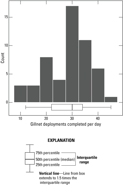
Representation of counts of gillnet deployments completed in a single day over the study period in Clear Lake, Lake County, California. The box represents the median and interquartile range (IQR), and the whiskers extend to 1.5 times the IQR.
Power values were estimated using the “simr” package in the R statistical computing environment (Green and MacLeod, 2016). The approach of simr involves Monte Carlo simulations based off of a GLMM fitted to count data (Green and MacLeod, 2016). The first step was constructing a GLMM to test the effect of year on counts of juvenile and adult Clear Lake Hitch in gillnet deployments. The effect of year was included in the GLMM as a fixed effect that was coded as an integer so that the model calculated a slope across years. The GLMM included gillnet deployment time (log[minutes]) as an offset to account for sampling effort and included region as a random effect to account for spatial dependencies. An OLRE was also included to account for zero inflation (Harrison, 2014). The GLMM was fit with a Poisson distribution. Mixed models are fit within simr via lme4. The R package “DHARMa” was used to generate information to evaluate the fit of the models (Hartig, 2018). DHARMa employs a simulation-based approach for residual diagnostics of mixed models.
Power values are calculated in simr by repeating the following three steps: (1) simulate new values for the response variable using the model provided; (2) refit the model to the simulated response; and (3) apply a statistical test to the simulated fit. In this setup, the tested effect is known to exist, so every positive test is a true positive, and every negative test is a Type II error. The power of the test can be calculated from the number of successes and failures at step three (Green and MacLeod, 2016). One thousand simulations were completed.
Data Sources
All fish and ancillary sampling data are available in a USGS data release (Palm and others, 2023). Water quality vertical profile data have been published separately in a USGS data release (Wulff and others, 2019). The Clear Lake outline was obtained from the State of California’s California Lakes dataset (California Department of Fish and Wildlife, 2024). Water temperature data shown in fig. 6 were obtained from the University of California, Davis (UCD, 2024; Lake Monitoring site = UA-06; Longitude: −122.8170, Latitude: 39.0610). Flow data on figure 6 were obtained from the U.S. Geological Survey, site 11449500 (U.S. Geological Survey, 2024).
Results and Discussion
A total of 1,529 gillnet deployments amounting to 60,697 minutes of sampling effort was completed during the study period (table 1). Individual gillnet deployments were broadly distributed across all three geographic arms of Clear Lake (fig. 2). Repeat samples associated with the ACS completed during 2021–23 accounted for 85 of the 782 (11 percent) gillnet deployments done during that period (table 2). Overall mean duration of individual gillnet deployments was 40 minutes (minimum = 9; maximum = 119; standard deviation = 10).
Table 1.
Summary of discrete measurements of key variables during Clear Lake Hitch sampling in Clear Lake, Lake County, California, 2017–23. Data summarized from Palm and others (2023).[°C, degrees Celsius; FNU, Formazin Nephelometric Units; mg/L, milligrams per Liter; µS/cm, microsiemens per centimeter; <, less than; µg/L, micrograms per liter]
Table 2.
Summary details of the adaptive cluster sampling (ACS) of Clear Lake Hitch in Clear Lake, Lake County, California, done during 2021–23. Data summarized from Palm and others (2023).[A second round of ACS was not done in 2022 because no Clear Lake Hitch were captured in the first round. N is the count of gillnet deployments. Abbreviation: No., number]
Gillnet deployments sampled across a range of water quality conditions (table 1). During gillnet deployments, mean water temperature ranged from 22 to 25 °C, and mean dissolved oxygen concentration ranged from 6 to 10 mg/L. The overall percentage of gillnet deployments with hypoxia (dissolved oxygen concentration <2.0 mg/L) was 14 percent during 2017–19 and 1 percent during 2021–23 (table 1). During gillnet deployments, mean specific conductance ranged from 266 to 405 µS/cm, mean turbidity ranged from 1 to 12 FNU, mean chlorophyll a concentration ranged from 2 to 9 µg/L, and mean pH ranged from 8 to 9.
The sampling effort captured a total of 986 individual Clear Lake Hitch, comprised of 390 juveniles and 596 adults (table 1). The repeat ACS samples completed during 2021–23 accounted for 102 of the 179 (57 percent) juvenile Clear Lake Hitch and 73 of the 165 (44 percent) adult Clear Lake Hitch captured during that period (table 2). The total number of juvenile Clear Lake Hitch captured per year ranged from 0 to 191, and the total number of adult Clear Lake Hitch captured per year ranged from 4 to 273 (table 1). As previously mentioned, counts of Clear Lake Hitch in individual gillnet deployments were highly zero inflated (fig. 7); juvenile Clear Lake Hitch were absent from 93 percent of gillnet deployments, and adult Clear Lake Hitch were absent from 89 percent of gillnet deployments (fig. 7). The maximum number of juvenile Clear Lake Hitch captured in a single gillnet deployment was 36, and the maximum number of adult Clear Lake Hitch captured in a single gillnet deployment was 77 (fig. 7). The smallest Clear Lake Hitch encountered was 119 mm and the largest was 385 mm.
Clear Lake Hitch Monitoring Evaluation
The model constructed to examine gillnet retention selectivity appears to have provided a good fit to the data, as indicated by deviance values and residual patterns. Null deviance, which indicates how the model fit the data with only the intercept, was 4,620. Model deviance, which indicates how the model fit the data with the SL size increments included as explanatory covariates, was 200. The very small model deviance compared to the very large null deviance indicates that the model provided a good fit to the data. Residuals were generally small with no underlying pattern, further suggesting that the model provided a good fit to the data (fig. 10). Inspection of the calculated retention curves indicated that each individual mesh size was effective for a specific size range of Clear Lake Hitch. However, collectively, the five mesh sizes effectively captured Clear Lake Hitch from approximately 120 mm SL to 375 SL (fig. 11), which generally matches the expected size ranges of age-1+ Clear Lake Hitch (Geary and Moyle, 1980; Moyle, 2002).
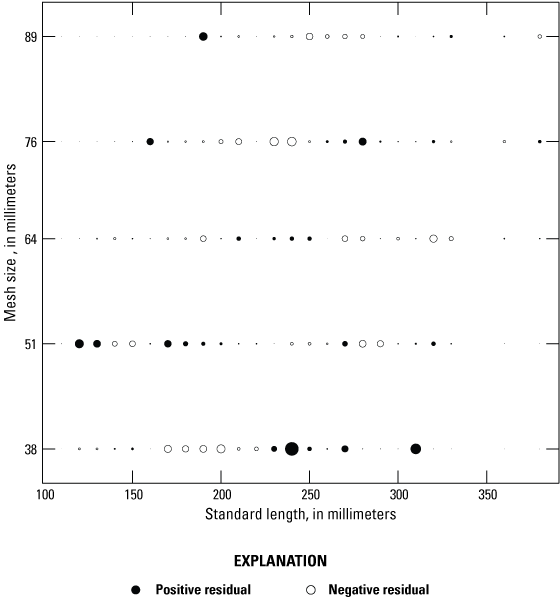
Deviance residual plot for the fitted retention curves for Clear Lake Hitch standard length sampled from Clear Lake, Lake County, California, across the five different sizes of mesh on the gillnets. The size of the filled black circles represents the magnitude of positive residuals, and the size of the filled white circles represents the magnitude of negative residuals. Data summarized from Palm and others (2023).

Fitted relative retention curves for Clear Lake Hitch standard length (SL) across the five different sizes of mesh used on the gillnets. Data summarized from Palm and others (2023).
Standardized Abundance Index
Both juvenile and adult Clear Lake Hitch were more frequently observed and more abundant in normoxic (dissolved oxygen concentration ≥2.0 mg/L) compared to hypoxic (dissolved oxygen concentration <2.0 mg/L) gillnet deployments during 2017–19 (fig. 12). Juvenile Clear Lake Hitch occurred in a total of 70 samples, only two (3 percent) of which were classified as hypoxic. Adult Clear Lake Hitch occurred in a total of 98 samples, only six (6 percent) of which were classified as hypoxic. The results of the GLMM indicated that counts of juvenile and adult Clear Lake Hitch were significantly higher in normoxic compared to hypoxic conditions (table 3; fig. 12). These results indicate that terminating gillnet deployments in hypoxic conditions starting in 2021 was warranted and should not be resumed. Based on the frequency of deployments performed in hypoxic habitat in 2017, implementing this change will meaningfully improve field operational efficiencies, up to approximately 20 percent or more.
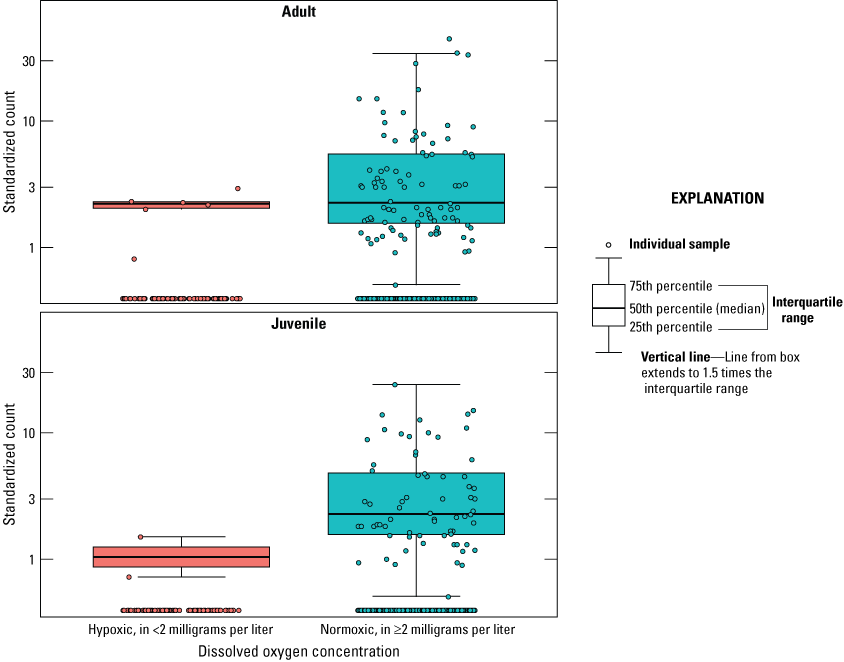
Representation of counts (log10 scale) of Clear Lake Hitch by life stage (juvenile or adult) captured in normoxic (blue; dissolved oxygen concentration ≥2.0 mg/L) and hypoxic (red; dissolved oxygen concentration <2.0 mg/L) habitat in Clear Lake, Lake County, California, during 2017–19. Boxplots were generated using only the non-zero counts. Counts were standardized to 60 minutes of deployment time. Horizontal jitter was added to the individual data points to reduce superimposition and improve visual interpretation. The box represents the median and interquartile range (IQR), and the whiskers extend to 1.5 times the IQR. Points represent individual samples. Data summarized from Palm and others (2023).
Table 3.
Results of the generalized linear mixed model that tested the effect of dissolved oxygen concentration on counts of juvenile and adult Clear Lake Hitch in gillnet deployments in Clear Lake, Lake County, California. Data summarized from Palm and others (2023).[OLRE, object-level random effect; SD, standard deviation; SE, standard error; <, less than]
There was no statistically significant effect of gillnet deployment scheme, surface versus mid-depth suspended, on counts of Clear Lake Hitch (table 4; fig. 13). Results of the model fit to the juvenile Clear Lake Hitch counts should be interpreted with caution because of sparse data (only three non-zero counts). These results indicate that the two deployment schemes generated redundant information and, therefore, terminating mid-depth suspended deployments would generate logistical efficiencies in the field.
Table 4.
Results of the generalized linear mixed model that tested the effect of gillnet deployment scheme (surface versus mid-depth suspended) on counts of juvenile and adult Clear Lake Hitch in Clear Lake, Lake County, California. Data summarized from Palm and others (2023).[SD, standard deviation; SE, standard error; <, less than]
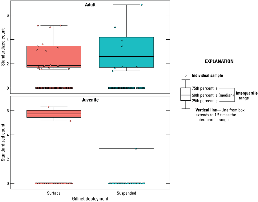
Representation of counts of Clear Lake Hitch by life stage (juvenile or adult) captured in surface versus mid-depth (suspended) gillnet deployments in Clear Lake, Lake County, California, during 2021–23. Boxplots were generated using only the non-zero counts. Counts were standardized to 60 minutes of deployment time. Horizontal jitter was added to the individual data points to reduce superimposition and improve visual interpretation. The box represents the median and interquartile range (IQR), and the whiskers extend to 1.5 times the IQR. Points represent individual samples. Data summarized from Palm and others (2023).
There was a statistically significant, albeit small, negative effect of hour of day on counts of juvenile and adult Clear Lake Hitch (table 5; fig. 14). The estimated coefficient values for hour of day were −0.1 and −0.2 for adult and juvenile Clear Lake Hitch, respectively (table 5). These coefficient values indicated that it took 10 hours into a day for adults and 6 hours into a day for juveniles for the cumulative effect to be greater than a fraction of an individual fish. These results indicate that there is no need to adjust future sampling effort by time of day because it would not generate meaningful operational efficiencies in the field.
Table 5.
Results of the generalized linear mixed model that tested the effect of hour of day on counts of juvenile and adult Clear Lake Hitch in gillnet deployments in Clear Lake, Lake County, California. Data summarized from Palm and others (2023).[OLRE, object-level random effect; SD, standard deviation; SE, standard error; <, less than]

Counts of Clear Lake Hitch by life stage (juvenile or adult) captured by hour of day in gillnet deployments in Clear Lake, Lake County, California. Boxplots were generated using only the non-zero counts (white circles are positive counts, and red circles are zero counts). Counts were standardized to 60 minutes of deployment time. Horizontal jitter was added to the individual data points to reduce superimposition and improve visual interpretation. The box represents the median and interquartile range (IQR), and the whiskers extend to 1.5 times the IQR. Points represent individual samples. Data summarized from Palm and others (2023).
The three candidate standardized abundance indices—nominal, normoxic, and normoxic without ACS—showed different absolute values but the same basic pattern among years (fig. 15). From 2017 to 2019, the nominal abundance index was smaller than the normoxic and normoxic without ACS indices, indicating that sampling hypoxic habitat biased abundance indices low because of how it inflated the count of gillnet deployments without Clear Lake Hitch present. The normoxic and normoxic without ACS indices were identical during 2017–19 because ACS was not implemented until 2021. From 2021 to 2023, the normoxic without ACS index was smaller than the nominal and normoxic indices. This outcome indicated that ACS biased abundance indices high because of how it inflated the number of gillnet deployments with Clear Lake Hitch present. The nominal and normoxic indices were virtually identical during 2021–23 because there was almost no sampling completed in hypoxic conditions during this time period. These results indicate that calculating unbiased standardized abundance indices should exclude hypoxic and ACS gillnet deployments.

Candidate abundance indices calculated as mean catch per unit effort (±95-percent confidence intervals) of Clear Lake Hitch life stages (juvenile or adult) in Clear Lake, Lake County, California. The three indices are as follows: nominal = all available sample data; normoxic = excludes sample data with dissolved oxygen concentration <2.0 mg/L; and without adaptive clustering sampling = normoxic sample data without adaptive cluster sampling. Data summarized from Palm and others (2023).
Length-Frequency Distribution
Length-frequency distributions across the three candidate scenarios—nominal, normoxic, and normoxic without ACS—showed very similar patterns (fig. 16). This result indicates that the dominant patterns in length-frequency distribution were largely insensitive to the variation in the number of individual Clear Lake Hitch captured across the scenarios. These results show that the approach for generating standardized length-frequency distributions should match that of the abundance indices by excluding hypoxic and ACS gillnet deployments.

Length-frequency distributions of Clear Lake Hitch standard length by year, sampled from Clear Lake, Lake County, California, for the same sampling scenarios considered as candidate abundance indices. The three scenarios are as follows: nominal = all available sample data; normoxic = excludes sample data with dissolved oxygen concentration <2.0 milligrams per liter (mg/L); and without adaptive cluster sampling = normoxic sample data without adaptive cluster sampling. Red reference lines denote 175 millimeters (mm), delineating juvenile (<175 mm) from adult (≥175 mm) Clear Lake Hitch. Data summarized from Palm and others (2023).
Power Analysis to Guide Future Efforts
The GLMMs constructed to be the foundations of the power analysis had reasonably good fits to the data, as inferred from diagnostic residual tests performed in DHARMa (model output and DHARMa test results are not shown but are available upon request). Based on these results, the models were deemed suitable for performing the power analysis.
Results of the power analysis indicated that power had a generally positive association with sample size and effect size (change in abundance; fig. 17). Results of the 6-year scenario were similar enough between adult and juvenile Clear Lake Hitch that the results could be generalized for both life stages (fig. 17). Power to detect a 5-percent change in abundance was below 80 percent for all scenarios considered. Power to detect a 10-percent change in abundance was above 80 percent for sampling effort scenarios ≥ N=100 gillnet deployments per year. Power to detect a 15- or 20-percent change in abundance was above 80 percent for sampling effort scenarios ≥ N=50 gillnet deployments per year. Power to detect a 25-percent change in abundance was above 80 percent for all sampling effort scenarios.
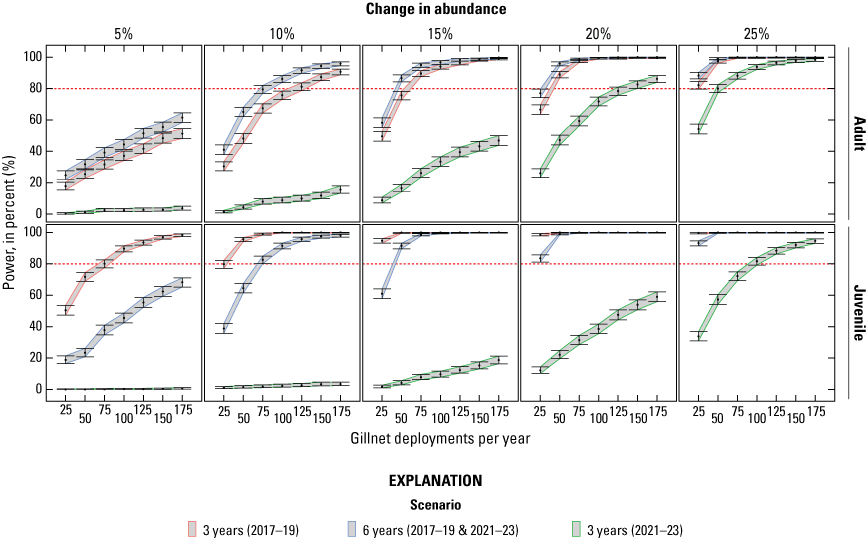
Power (mean ±95-percent confidence intervals) to detect 5-, 10-, 15-, 20-, or 25-percent changes in abundance of Clear Lake Hitch life stages (juvenile or adult) sampled from Clear Lake, Lake County, California, for three scenarios calculated over a range of gillnet deployment sample sizes per year. Horizontal red reference lines denote 80-percent power. Data summarized from Palm and others (2023).
Results differed between the two 3-year scenarios (fig. 17). The scenario involving 2017–19 showed results generally like the 6-year scenario. However, the scenario involving 2021–23 showed consistently lower power than the two other scenarios. This result was obtained because variability in abundance among years was lower for the 2021–23 scenario compared to the 2017–19 and the 6-year scenario (fig. 15). This finding may partially reflect how power to detect changes may be more stochastic as populations decrease in size, and individuals become increasingly difficult to detect. Eighty percent power was exceeded (confidence intervals not overlapping 80-percent power) in the 2021–23 scenario only at a 25-percent change in abundance and sampling effort scenarios ≥ N=100 gillnet deployments per year.
Conclusions
In 2017, the U.S. Geological Survey, in cooperation with the U.S. Fish and Wildlife Service, initiated a monitoring program to generate information annually on relative abundance and size structure of Clear Lake Hitch (Lavinia exilicauda chi), a minnow endemic to Clear Lake, Lake County, California, that is listed as a threatened species under the California Endangered Species Act and has been petitioned for listing under the United States Endangered Species Act. The monitoring program was organized around a conceptual life cycle diagram of the Clear Lake Hitch, focused on life stages approximately ≥1 year of age, and included a probabilistic sampling design that involved approximately 10 days of gillnet sampling in early summer.
The evaluation in this report of monitoring program activities from 2017 to 2023 indicated sampling Clear Lake Hitch to assess population status and trends is challenging but can be accomplished with appropriate effort and resources. The results of the analysis indicated the following: (1) gillnets used in the study were effective at capturing Clear Lake Hitch aged 1 year or more; (2) the study design was effective at generating information needed to characterize Clear Lake Hitch relative abundance and size structure, and meaningful operational efficiencies can be obtained through terminating gillnet deployments in hypoxic habitat, terminating mid-depth suspended gillnet deployments, and terminating ACS; and (3) future sampling can be scaled to approximately 4–7 days of effort and maintain at least 80-percent confidence in detecting at minimum a 25-percent change in abundance, assuming past work productivity is maintained, and future data are typical of previous data.
The following actions have high potential for facilitating effective status and trends monitoring of Clear Lake Hitch:
-
• Future sampling and, by association, generation of standardized abundance indices and length-frequency information, need not involve hypoxic, suspended mid-depth, and ACS gillnet deployments.
-
• Effort should be made to estimate total population size at some frequency, perhaps once every 6 years. Estimating population size will require novel thinking and substantial resources but should be a high priority in order to provide context and scale for interpreting the standardized abundance indices.
-
• Effort should be made to develop standardized methods for assessing status and trends of Clear Lake Hitch younger than 1 year of age. Examples include quantifying abundance of adult spawners in streams and quantifying abundance of juvenile life stages in streams and the lake. Information on these life stages is lacking but is essential to understand the key factors driving population dynamics and long-term viability of Clear Lake Hitch.
-
• Future program evaluations should occur at a frequency of at least every 6 years. Evaluations may need to be completed at shorter intervals if the population appears to be in grave condition, shows variability atypical of the data included in this assessment, or if information needs change.
References Cited
Bates, D., Mächler, M., Bolker, B.M., and Walker, S.C., 2015, Fitting linear mixed-effects models using lme4: Journal of Statistical Software, v. 67, no. 1, p. 1–48, accessed December 13, 2024, at https://doi.org/10.18637/jss.v067.i01.
Bonar, S.A., and Hubert, W.A., 2002, Standard sampling of inland fish—Benefits, challenges, and a call for action: Fisheries, v. 27, no. 3, p. 10–16, accessed December 13, 2024, at https://doi.org/10.1577/1548-8446(2002)027%3C0010:SSOIF%3E2.0.CO;2.
Bue, C.D., 1963, Principal lakes of the United States: U.S. Geological Survey Circular 476, 22 p., accessed December 13, 2024, at https://doi.org/10.3133/cir476.
California Department of Fish and Wildlife [CDFW], 2014, Report to the Fish and Game Commission, A status review of Clear Lake Hitch (Lavinia exilicauda chi): California Department of Fish and Wildlife report, [variously paged; 378 p.], accessed December 13, 2024, at https://nrm.dfg.ca.gov/FileHandler.ashx?DocumentID=86747.
California Department of Fish and Wildlife [CDFW], 2024, California Lakes: California Department of Fish and Wildlife database, accessed December 13, 2024, at https://data.cnra.ca.gov/dataset/california-lakes.
Feyrer, F., 2019, Observations of the spawning ecology of the imperiled Clear Lake Hitch: California Fish and Game, v. 105, no. 4, p. 225–232, accessed December 13, 2024, at https://nrm.dfg.ca.gov/FileHandler.ashx?DocumentID=174808&inline.
Feyrer, F., Hobbs, J., Acuna, S., Mahardja, B., Grimaldo, L., Baerwald, M., Johnson, R.C., and Teh, S., 2015, Metapopulation structure of a semi-anadromous fish in a dynamic environment: Canadian Journal of Fisheries and Aquatic Sciences, v. 72, no. 5, p. 709–721. [Available at https://doi.org/10.1139/cjfas-2014-0433.]
Feyrer, F., Whitman, G., Young, M., and Johnson, R.C., 2019a, Strontium isotopes reveal ephemeral streams used for spawning and rearing by an imperiled potamodromous cyprinid, Clear Lake Hitch Lavinia exilicauda chi: Marine and Freshwater Research, v. 70, no. 12, p. 1689–1697. [Available at https://doi.org/10.1071/MF18264.]
Feyrer, F., Young, M., Patton, O., and Ayers, D., 2019b, Dissolved oxygen controls summer habitat of Clear Lake Hitch (Lavinia exilicauda chi), an imperiled potamodromous cyprinid: Ecology of Freshwater Fish, v. 29, no. 2, p. 188–196. [Available at https://doi.org/10.1111/eff.12505.]
Geary, R.E., and Moyle, P.B., 1980, Aspects of the ecology of the hitch, Lavinia exilicauda (Cyprinidae), a persistent native cyprinid in Clear Lake, California: The Southwestern Naturalist, v. 25, no. 3, p. 385–390, accessed December 13, 2024, at https://doi.org/10.2307/3670695.
Gerrodette, T., 1987, A power analysis for detecting trends: Ecology, v. 68, no. 5, p. 1364–1372, accessed December 13, 2024, at https://doi.org/10.2307/1939220.
Green, P., and MacLeod, C.J., 2016, SIMR—An R package for power analysis of generalized linear mixed models by simulation: Methods in Ecology and Evolution, v. 7, no. 4, p. 493–498, accessed December 13, 2024, at https://doi.org/10.1111/2041-210X.12504.
Griffith, G.E., Omernik, J.M., Smith, D.W., Cook, T.D., Tallyn, E., Moseley, K., and Johnson, C.B., 2016, Ecoregions of California (poster): U.S. Geological Survey Open-File Report 2016–1021, with map, scale 1:1,100,000, accessed December 13, 2024, at https://doi.org/10.3133/ofr20161021.
Harrison, X.A., 2014, Using observation-level random effects to model overdispersion in count data in ecology and evolution: PeerJ, v. 2, 19 p. [Available at https://doi.org/10.7717/peerj.616.]
Hartig, F., 2018, DHARMa—Residual diagnostics for hierarchical (multi-level/mixed) regression models: R package, version 0.4.6, accessed December 13, 2024, at https://cran.r-project.org/web/packages/DHARMa/index.html.
Hubert, W.A., Pope, K.L., and Dettmers, J.M., 2012, Passive capture techniques, in Zale, A.V., Parrish, D.L., and Sutton, T.M., eds., Fisheries techniques (3d ed.): Bethesda, Md., American Fisheries Society, p. 223–265. [Available at https://digitalcommons.unl.edu/ncfwrustaff/111.]
Maunder, M.N., and Punt, A.E., 2004, Standardizing catch and effort data—A review of recent approaches: Fisheries Research, v. 70, nos. 2–3, p. 141–159, accessed December 13, 2024, at https://doi.org/10.1016/j.fishres.2004.08.002.
Maxwell, D., and Jennings, S., 2005, Power of monitoring programmes to detect decline and recovery of rare and vulnerable fish: Journal of Applied Ecology, v. 42, no. 1, p. 25–37. [Available at https://doi.org/10.1111/j.1365-2664.2005.01000.x.]
Millar, R.B., and Holst, R., 1997, Estimation of gillnet and hook selectivity using log-linear models: ICES Journal of Marine Science, v. 54, no. 3, p. 471–477. [Available at https://doi.org/10.1006/jmsc.1996.0196.]
Myrick, C.A., and Cech, J.J., 2000, Swimming performances of four California stream fishes—Temperature effects: Environmental Biology of Fishes, v. 58, p. 289–295, accessed December 13, 2024, at https://doi.org/10.1023/A:1007649931414.
Neumann, R.M., and Allen, M.S., 2007, Size structure, chap. 9 of Guy, C.S., and Brown, M.L., eds., Analysis and interpretation of freshwater fisheries data: American Fisheries Society, Bethesda, Md., p. 375–421. [Available at https://fisheries.org/docs/books/55049C/9.pdf.]
Nobriga, M.L., Feyrer, F., Baxter, R.D., and Chotkowski, M., 2005, Fish community ecology in an altered river delta—Spatial patterns in species composition, life history strategies, and biomass: Estuaries, v. 28, no. 5, p. 776–785, accessed December 13, 2024, at https://doi.org/10.1007/BF02732915.
Palm, D.P., Clause, J.K., Steinke, D.A., Young, M.J., Feyrer, F.V., and Santana, L., 2023, Abundance and distribution of fishes in Clear Lake, Lake County, California (ver. 2.0, December 2024): U.S. Geological Survey data release, accessed December 13, 2024, at https://doi.org/10.5066/P9KXAMKP.
R Core Team, 2020, R—The R project for statistical computing: Vienna, Austria, R Foundation for Statistical Computing, accessed February 2020, at https://www.r-project.org.
Radinger, J., Britton, J.R., Carlson, S.M., Magurran, A.E., Alcaraz‐Hernández, J.D., Almodóvar, A., Benejam, L., Fernández‐Delgado, C., Nicola, G.G., Oliva‐Paterna, F.J., Torralva, M., and García-Berthou, E., 2019, Effective monitoring of freshwater fish: Fish and Fisheries, v. 20, no. 4, p. 729–747, accessed December 13, 2024, at https://doi.org/10.1111/faf.12373.
Reynolds, J.H., Knutson, M.G., Newman, K.B., Silverman, E.D., and Thompson, W.L., 2016, A road map for designing and implementing a biological monitoring program: Environmental Monitoring and Assessment, v. 188, no. 7, article 399, 25 p. [Available at https://doi.org/10.1007/s10661-016-5397-x.]
Říha, M., Prchalová, M., Brabec, M., Draštík, V., Muška, M., Tušer, M., Bartoň, D., Blabolil, P., Čech, M., Frouzová, J., Holubová, M., Jůza, T., Moraes, K.R., Rabaneda-Bueno, R., Sajdlová, Z., Souza, A.T., Šmejkal, M., Vašek, M., Vejřík, L., Vejříková, I., Peterka, J., and Kubečka, J., 2023, Calibration of fish biomass estimates from gillnets—Step towards broader application of gillnet data: Ecological Indicators, v. 153, 14 p. [Available at https://doi.org/10.1016/j.ecolind.2023.110425.]
Steinke, D.A., Young, M.J., and Feyrer, F.V., 2019, Abundance and distribution of fishes in the Northern Sacramento–San Joaquin Delta, California, 2017–2018 (ver. 1.1, December 2019): U.S. Geological Survey data release, accessed December 13, 2024, at https://doi.org/10.5066/P9FUQXJL.
Thompson, S.K., 1990, Adaptive cluster sampling: Journal of the American Statistical Association, v. 85, no. 412, p. 1050–1059. [Available at https://doi.org/10.1080/01621459.1990.10474975.]
Turk, P., and Borkowski, J.J., 2005, A review of adaptive cluster sampling—1990–2003: Environmental and Ecological Statistics, v. 12, no. 1, p. 55–94, accessed December 13, 2024, at https://doi.org/10.1007/s10651-005-6818-0.
University of California, Davis [UCD], 2024, Clear Lake data: University of California, Davis, Tahoe Environmental Research Center database accessed December 13, 2024, at https://tercdev.github.io/Clear_Lake_Website_Data_Visualization/data-archive.
U.S. Geological Survey, 2024, USGS water data for the Nation: U.S. Geological Survey National Water Information System database, accessed August 29, 2024, at https://doi.org/10.5066/F7P55KJN.
U.S. Geological Survey, 2025a, USGS Fundamental Science Practices (FSP) Home, U.S. Geological Survey web page, accessed March 10, 2025, at https://www.usgs.gov/office-of-science-quality-and-integrity/fundamental-science-practices.
U.S. Geological Survey, 2025b, USGS Data Management, U.S. Geological Survey web page, accessed March 10, 2025, at https://www.usgs.gov/data-management.
Valentine, D.A., Young, M.J., and Feyrer, F., 2020, Sacramento Pikeminnow migration record: Journal of Fish and Wildlife Management, v. 11, no. 2, p. 588–592. [Available at https://doi.org/10.3996/JFWM-20-038.]
Wagner, T., Irwin, B.J., Bence, J.R., and Hayes, D.B., 2013, Detecting temporal trends in freshwater fisheries surveys—Statistical power and the important linkages between management questions and monitoring objectives: Fisheries, v. 38, no. 7, p. 309–319, accessed December 13, 2024, at https://doi.org/10.1080/03632415.2013.799466.
Wulff, M.L., Feyrer, F.V., and Young, M.J., 2022, Gill-net selectivity for fifteen fish species of the upper San Francisco Estuary: San Francisco Estuary and Watershed Science, v. 20, no. 2., 10 p. [Available at https://doi.org/10.15447/sfews.2022v20iss2art4.]
Wulff, M.L., Steinke, D.A., Young, M.J., Clause, J.K., and Feyrer, F.V., 2019, Water quality vertical profiles in Clear Lake, Lake County, California, 2017–2019 (ver. 4.0, May 31, 2024): U.S. Geological Survey data release, accessed December 13, 2024, at https://doi.org/10.5066/P9L40JG3.
Young, M.J., Larwood, V., Clause, J.K., Bell-Tilcock, M., Whitman, G., Johnson, R., and Feyrer, F., 2022, Eye lenses reveal ontogenetic trophic and habitat shifts in an imperiled fish, Clear Lake Hitch (Lavinia exilicauda chi): Canadian Journal of Fisheries and Aquatic Sciences, v. 79, no. 1, p. 21–30, accessed December 13, 2024, at https://doi.org/10.1139/cjfas-2020-0318.
Datum
Horizontal coordinate information is referenced to the North American Vertical Datum of 1983 (NAVD 83).
Supplemental Information
Specific conductance is in microsiemens per centimeter at 25 degrees Celsius (µS/cm at 25 °C).
Concentrations of chemical constituents in water are in either milligrams per liter (mg/L) or micrograms per liter (µg/L).
For more information concerning the research in this report, contact the
Director, California Water Science Center
U.S. Geological Survey
6000 J Street, Placer Hall
Sacramento, California 95819
https://www.usgs.gov/centers/ca-water/
Publishing support provided by the U.S. Geological Survey
Science Publishing Network, Sacramento Publishing Service Center
Disclaimers
Any use of trade, firm, or product names is for descriptive purposes only and does not imply endorsement by the U.S. Government.
Although this information product, for the most part, is in the public domain, it also may contain copyrighted materials as noted in the text. Permission to reproduce copyrighted items must be secured from the copyright owner.
Suggested Citation
Feyrer, F., Young, M.J., Huntsman, B., Violette, V., Clause, J.K., Buxton, J., Palm, D., Wulff, M., Gronemyer, J., and Santana, L., 2025, Gillnet sampling methods for monitoring status and trends of Clear Lake Hitch in Clear Lake, Lake County, California: U.S. Geological Survey Open-File Report 2025–1018, 26 p., https://doi.org/10.3133/ofr20251018.
ISSN: 2331-1258 (online)
Study Area
| Publication type | Report |
|---|---|
| Publication Subtype | USGS Numbered Series |
| Title | Gillnet sampling methods for monitoring status and trends of Clear Lake Hitch in Clear Lake, Lake County, California |
| Series title | Open-File Report |
| Series number | 2025-1018 |
| DOI | 10.3133/ofr20251018 |
| Publication Date | May 02, 2025 |
| Year Published | 2025 |
| Language | English |
| Publisher | U.S. Geological Survey |
| Publisher location | Reston, VA |
| Contributing office(s) | California Water Science Center |
| Description | Report: viii, 26 p.; Data Release |
| Country | United States |
| State | California |
| County | Lake County |
| Other Geospatial | Clear Lake |
| Online Only (Y/N) | Y |