

Groundwater Budget for the Surficial Aquifer Surrounding Lake Nokomis, Minneapolis, Minnesota
Links
- Document: Report (1.3 MB pdf) , HTML , XML
- Dataset: USGS National Water Information System database - USGS water data for the Nation
- NGMDB Index Page: National Geologic Map Database Index Page (html)
- Download citation as: RIS | Dublin Core
Acknowledgments
Funding for this study was provided by the Minnesota Environment and Natural Resources Trust Fund as recommended by the Legislative-Citizen Commission on Minnesota Resources and the U.S. Geological Survey’s Cooperative Matching Funds program. The author would like to thank the partners of this study that provided technical assistance, including staff from the University of Minnesota, Minnesota Geological Survey, and the Minnesota Department of Natural Resources.
Andrew Berg, Hayden Lockmiller, Jared Trost, and Kim Perkins (U.S. Geological Survey) provided data collection and processing assistance for this report.
Abstract
During prolonged periods of above-average precipitation, rising groundwater levels have the potential to cause damage to and interfere with underground infrastructure and building foundations. To understand the relations between precipitation and groundwater in the vicinity of Lake Nokomis, the U.S. Geological Survey, in collaboration with the University of Minnesota, quantified five components of the groundwater budget: groundwater recharge, change in surficial aquifer storage, surficial aquifer groundwater discharge to Lake Nokomis, groundwater evapotranspiration, and groundwater discharge to underlying bedrock aquifers. Field data, geologic records, and empirical calculation methods were used to quantify groundwater budget components for April 2023 through April 2024. Lake water budget data indicate that Lake Nokomis is a flowthrough system during periods with no outflow through the weir, with groundwater inputs equal to outputs. Roughly 40 percent of precipitation that fell in the study area was added to the surficial aquifer as recharge. Uncertainty in the vertical hydraulic conductivity resulted in wide-ranging estimates (spanning three orders of magnitude) of water discharging from the surficial aquifer to the underlying bedrock aquifer. Drought conditions persisted for the duration of this study and were not representative of the conditions that motivated this study. This study is a start towards understanding relations between precipitation, Lake Nokomis levels, and groundwater levels that could affect local underground infrastructure.
Introduction
Between 2013 and 2019, the metropolitan area surrounding Minneapolis, Minnesota, experienced the equivalent of 8 years of rain in a 7-year span (Schaufler and others, 2022). During this time, area residents became concerned about the effects of this increased rainfall on city and residential infrastructure. Information about groundwater responses to precipitation in the vicinity of Lake Nokomis could be useful for community resiliency planning for future wet periods. Schaufler and others (2022) were tasked by local decision makers with providing a historical account of the area and its development and quantifying the meteorological events that may be contributing to the infrastructure problems in the area surrounding Lake Nokomis. Schaufler and others (2022) also identified areas where data and understanding of the area were lacking, mainly of the local geology and hydrogeological system. The U.S. Geological Survey (USGS) measured and calculated components of the surficial aquifer’s water balance as part of a larger study led by the University of Minnesota (Legislative-Citizen Commission of Minnesota Resources, 2021) to provide hydrogeological data and analysis to the area surrounding Lake Nokomis.
Lake Nokomis is an urban lake in the southeast corner of Minneapolis, Minn. (fig. 1). The lake is just south of Minnehaha Creek and is connected via a dam and weir. Prior to European settlement, the lake and surrounding area was a shallow lake, wetland, and peat bog complex. The lake was excavated in the early 20th century. The excavated material was used to fill in the surrounding area to make it more suitable for development (Schaufler and others, 2022). The groundwater budget analysis in this report differs from the timeframe discussed in Schaufler and others (2022) in that the area experienced drought conditions for the length of the study (National Oceanic and Atmospheric Administration, 2024). Analysis in this report responds to a component of the recommendations within Schaufler and others (2022) to quantify the geological and hydrogeological setting of the Lake Nokomis area.
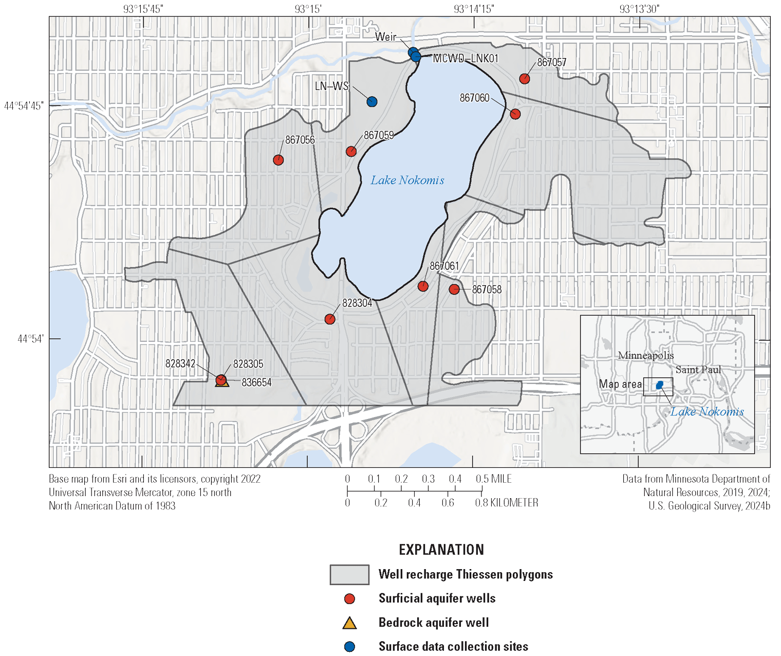
Map of the area surrounding Lake Nokomis, Minneapolis, Minnesota.
Purpose and Scope
This report describes data collection and analysis for the area surrounding Lake Nokomis in Minneapolis, Minn., by the USGS, in cooperation with the University of Minnesota. The data collected for this report are available in the National Water Information System database (U.S. Geological Survey, 2024b). This report describes measurement and estimation of five water budget components, including groundwater recharge, change in surficial aquifer storage, surficial aquifer groundwater discharge to Lake Nokomis, groundwater evapotranspiration, and groundwater discharge to underlying bedrock aquifers. Data were collected and water budget estimates were made for March 2023 to April 2024.
Methods
To quantify the groundwater budget, several types of data were collected. Nine monitoring wells (eight surficial aquifer wells and one bedrock aquifer well), three preexisting and six installed for this study, were used to measure water elevation data surrounding the lake (fig. 1). Four wells were in the lowland areas and six wells were in upland areas near the lake. Two wells, 828304 and 828305, were installed in November 2017. 836654 was installed in March of 2019. The remaining wells were installed in February 2023. Data collection at wells 828304, 828305, and 836654 was ongoing when the study period began (table 1). 828342 and 836654 were used to define glacial deposits and calculate the downward gradient between the surficial and bedrock aquifers. Well characteristics and aquifer information are provided in table 2. A weather station, LN–WS, which collected precipitation, solar radiation, and temperature, was also installed in the open field along the west side of the lake. A pressure transducer (MCWD–LNK01) was installed in the lake by the Minnehaha Creek Watershed District (MCWD) to measure the lake stage elevation (Beck, 2023) (fig. 1).
Table 1.
Site identifiers, summary of continuous data collected, and descriptions of how those data were used to calculate water budget components for Lake Nokomis and groundwater in 2023.[ID, identifier; NA, not applicable; dates shown in month/day/year format]
Refer to equations 1 and 2.
Table 2.
Study well identifiers, land surface elevation, open intervals, average water level, and aquifer classification.[USGS, U.S. Geological Survey; ID, identifier; MUN, Minnesota unique well number; ft, foot; NAVD 88, North American Vertical Datum 1988; BLS, below land surface; NA, not applicable dates shown in month/day/year format]
The full groundwater system budget was calculated for the period when all data were available. Lake stage elevation was collected from April 27 to October 24, 2023 (hereafter referred to as the “lake period”). Components from equations 2 and 3 were calculated for April 17, 2023, to March 5, 2024 (hereafter referred to as the “study period”). This report describes numbered days (elapsed time) for certain time periods. These numbered days refer to a count of days from December 31, 2022, so January 1, 2023, is day 1. The weather station LN–WS was installed April 17, 2023, and was the limiting dataset to calculate recharge. Daily mean elevation values for groundwater and lake levels were used to make all calculations to smooth out noise in the data (U.S. Geological Survey, 2024b).
Well 867057 had a substantial data gap from June 15 to October 3, 2023 (fig. 2). To fill this data gap, a linear regression analysis was done between daily mean elevation values for wells 867057 and 867056. The hydrograph at well 867056 was most like the hydrograph at well 867057 before and after the data gap compared to all other wells in the study. The regression analysis included daily mean water elevations from wells 867056 and 867057 from March 5 to June 15, 2023, and October 4, 2023, to March 5, 2024, to fill the data gap for well 867057 for June 15 to October 4, 2024. The regression equation is listed below (eq. 1). The coefficient of determination of the equation is 0.92881798. The elevation values predicted by the regression equation were all within 0.03 of a foot of discrete water level measurements made in well 867057 during the period of lost data.
whereY
is the daily average water elevation in well 867057, and
X
is the daily average water elevation in well 867056.
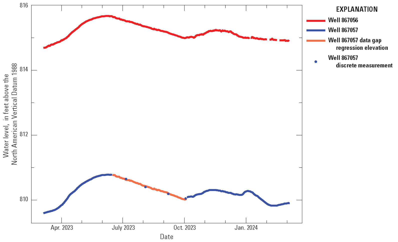
Hydrographs for wells 867056 and 867057 with data gap filled with regression data for missing data period from June 15 to October 3, 2023.
Conceptual Model
This study focuses on the area surrounding Lake Nokomis. The area where the five groundwater budget components were measured and calculated using equations 2 and 3 are the well Thiessen polygons shown in figure 1. Lateral fluxes in and out of the study area were assumed to be equal; therefore, no lateral flux term is present in equation 3. Equation 2 is a water budget equation for the lake itself. One of the variables, QGWLake, was used in equation 3 for the groundwater system.
whereQGWLake
is discharge from the groundwater system to the lake,
E
is evaporation out of the lake,
QOutlet
is discharge out of the lake via the weir,
∆SLake
is the change in storage in the lake,
P
is precipitation into the lake,
RO
is runoff into the lake,
Err
is the error in the calculation (this is the difference between the left and right sides of the equation),
R
is surficial aquifer recharge,
ETGW
is evapotranspiration from the groundwater system,
∆SGW
is change in storage of the surficial groundwater system, and
GWAquifer flux
is the flux of groundwater between the surficial aquifer and the underlying bedrock aquifer.
Lake Budget
All components of the lake budget were calculated during the lake period when lake stage elevation was measured (table 3). Lake elevations never rose enough for the weir at the lake’s outlet to be opened. Thus, “QOutlet” is equal to zero in table 3. Lake elevation responses to 24-hour precipitation of at least 0.5 inch were compared to evaluate whether runoff was contributing a substantial amount of water to the lake. If runoff was a major contribution to the lake, lake level increases would be consistently larger than precipitation depths. Nine precipitation events were analyzed. The mean difference between precipitation depth and lake level rise was 0.07 inch, and zero was within one standard deviation of the mean difference. Based on this analysis, runoff was determined to be a very minor contribution to the lake, and so a zero value was used when calculating equation 2.
Table 3.
Stage and volumetric Lake Nokomis budget calculation for April 27 to October 24, 2023.[QGWLake, groundwater discharge to the lake; Hamon, evapotranspiration equation from Hamon (1961); ft, feet; Jensen-Haise, Jensen-Haise equation from McGuinness and Bordne (1972); PET, potential evapotranspiration; NA, not applicable; QOutlet, outlet discharge; ft3, cubic feet; ∆SLake, change in storage of the lake; ft2, square feet; ft3, cubic feet; Mft3, million cubic feet]
A measurement of the surficial area of Lake Nokomis was needed to calculate the volumetric change of water in the lake. Two light detection and ranging (lidar) surveys have been conducted in the area that include the Lake Nokomis area. One was completed in November 2011 and the second was completed in May 2022 (U.S. Geological Survey, 2024a). Using digital elevation models (DEMs) created from the lidar data, the elevation of the lake was determined for the day the data were collected by analyzing the elevation values for the area of the lake within each DEM. In ArcGIS Pro, the Contour tool was used to create contour lines for the DEMs that would include the lake elevation determined from the DEMs. These contour lines were isolated, then turned into a polygon feature class so that the area of the lake at that elevation could be measured in square meters (Esri, 2024). These measurements were then converted to square feet. The elevation of the lake for the 2022 survey was 815.12 feet above the North American Vertical Datum of 1988 (NAVD 88) with an area of 9,039,637 square feet (ft2). The elevation for the 2011 survey was 813.98 ft NAVD 88 with an area of 8,864,058 ft2. The average of the two DEM-measured areas was 8,951,847 ft2 and was used to make volumetric calculations. The maximum lake elevation measured during data collection was 814.38 ft NAVD 88. The minimum lake elevation measured was 812.84 ft NAVD 88 (Beck, 2023). Higher-resolution lake bathymetry data could potentially improve the accuracy of the calculated lake area.
Change in Lake Storage of Lake Nokomis
The change in lake storage from April 27 to October 24, 2023, was calculated by subtracting the daily average lake stage elevation on October 24, 2023, from the daily average lake stage elevation on April 27, 2023 (table 3)
Evaporation
To find suitable potential evapotranspiration equations (PET) equations, literature from similar studies in Minnesota were considered. A recent USGS study in the Minneapolis metropolitan area evaluated multiple evapotranspiration equations and compared them to a class A pan evaporation measurement (Jones and others, 2016). Based on Jones and others (2016), and other data collected during this study, two different evaporation equations were selected to calculate evaporation from Lake Nokomis because the required data were available and, based on Jones and others (2016), they represent the high and low ends of the range of possible evaporation from the lake. The low end of lake evaporation was calculated using the Hamon equation (Hamon, 1961). The high end of lake evaporation was calculated using the Jensen-Haise equation (as in McGuinness and Bordne, 1972). Evaporation values obtained by way of these two equations were similar in magnitude to the values obtained in Jones and others (2016). The variables needed for the Hamon (1961) method, day length (D) and average temperature (Ta), are shown in equation 4. The Jensen-Haise method (as in McGuinness and Bordne, 1972) is shown in equation 6 and requires incident shortwave radiation (Rs) and average temperature (Ta).
wherePET
potential evapotranspiration, in centimeters per day;
D
is the hours of daylight in a day;
SVD
is saturated vapor density, in grams per cubic meter;
Ta1
is mean air temperature, in degrees Celsius;
Ta2
is mean air temperature, in degrees Fahrenheit; and
Rs
is incident shortwave radiation, in calories per square centimeter per day.
Data for calculation of evaporation with the Hamon equation were collected at the weather station LN–WS. Air temperature was measured at LN–WS directly in 15-minute increments. To obtain hours of daylight, solar radiation data were used. The period for each day where the solar radiation value is not 0 was counted as hours of daylight. This parameter was also measured every 15 minutes, so a non-zero measurement counts as 0.25 hour of daylight. The number of quarter hours of sunlight was summed to get the total hours of sunlight per day.
The same LN–WS data were also used to calculate evaporation with the Jensen-Haise equation (eq. 6). Temperature was converted from degrees Celsius to degrees Fahrenheit, and solar radiation was converted from millijoules per square meter to calories per square meter per day.
Precipitation
Precipitation was measured at the weather station LN–WS in 15-minute intervals as depth in inches. The total amount of precipitation added to the lake was determined by summing the total amount of rain that was measured from April 27 to October 24, 2023, converting that amount to feet, then multiplying that amount of rain by the average area of the lake (8,951,847 ft2).
Groundwater Budget
Eight monitoring wells were used for this study were used to represent a recharge contributing area surrounding Lake Nokomis (fig. 1 and table 1). The outer boundary of the recharge contributing area was assumed to be the same as the outer boundary of the surface watershed boundary. These areas were created using Thiessen polygons. The Thiessen polygons were created using the Create Thiessen Polygons tool in ArcGIS Pro. The Thiessen polygons extend just south of wells 828305 and 836654, but the watershed of the lake extends much farther to the south (Schaufler and others, 2022). This study is only concerned with the area surrounding the lake; therefore, an arbitrary southern border was chosen. The Lake Nokomis watershed was delineated by the MCWD (Minnehaha Creek Watershed District, 2022). This polygon shapefile was used in ArcGIS Pro to clip the Thiessen polygons so that their borders did not exceed that of the watershed area. The Minnesota Department of Natural Resources provided a shapefile of the outline of Lake Nokomis (Minnesota Department of Natural Resources, 2019). The Erase tool in ArcGIS Pro was used to remove the outline of the lake from the polygons (Esri, 2024). With the contributing representative recharge area of each well established, the water table fluctuation method was used to analyze each well hydrograph to determine the amount of recharge (Healy, 2010).
Groundwater recharge was calculated for each continuous well hydrograph using a master recession curve (MRC) and episodic master recession (EMR) technique described in Nimmo and Perkins (2018). Supporting R scripts and instructions for the application of this method to data are available through the U.S. Geological Survey (2025). The user-defined parameters for MRC analysis for each well are shown in table 4. Descriptions of the parameters are available in table 2 of Nimmo and Perkins (2018). The user-defined parameters for EMR analysis for each well are shown in table 5. Descriptions of the parameters are available in table 4 of Nimmo and Perkins (2018). These parameters were input into each R script to calculate the amount of recharge. These parameters were determined by analyzing the well hydrographs along with a time-series plot of the cumulative precipitation data collected at the weather station LN–WS. The basic concept for this analysis is determining the minimum amount of rainfall that causes a response in the hydrograph and the amount of time it takes for that response to happen. The input files used for the Nimmo and Perkins (2018) R scripts consist of comma separated value files that contain three columns of data. The first column is an elapsed time value, for this study, of the number of days since December 31, 2022; the second column is the water elevation, in feet NAVD 88; and the third column is a cumulative sum of the precipitation in inches measured at the weather station LN–WS. The daily mean elevation was used for analysis for all hydrograph analyses. The EMR program outputs a comma separated value file that itemizes the hydrograph into episode and non episode events as rows. For episode events, the important information for this study were the start and end dates, amount of recharge, and a recharge precipitation ratio (RPR). The EMR output quantified events that did not match with the timeframe during which lake stage elevation data were collected. To obtain total recharge amounts for this period for each well, the RPR was used. Lake stage elevation data collection ended on day 297. All well hydrographs had a recharge event that started before and ended after this date. The amount of precipitation was summed from the event start date to day 297 and then multiplied by the RPR of that event to determine how much recharge happened from the beginning date of the last event until day 297. Total recharge volumes for each well are listed in table 6.
Table 4.
Master recession curve (Nimmo and Perkins, 2018) inputs used to calculate recharge for each well surrounding Lake Nokomis.[resplimits, recharge response limits; throughorigin, force fit through origin; mindrytime, minimum duration of interval between significant precipitation and recession start; maxdelprecip, maximum amount of precipitation considered negligible; tslength, duration of slope elements for linearization; maxtick, maximum total uptick within a linearized slope element; binsize, bin size for lumping of change in recharge over change in time for fitting (0 for no binning); maxslope, maxmum allowable change in recharge over change in time for fitting; xlimresp, x-axis limits for response graphs; ylimresp, y-axis limits of response graphs; ylimprecip, y-axis limits for precip. graphs; xlimsl, x-axis limits for slope graphs; ylimsl, y-axis limits for slope graphs; annotated_specs, put specifications on master recession curve plot]
Table 5.
Episodic master recession (Nimmo and Perkins, 2018) inputs used to calculate recharge for each well surrounding Lake Nokomis.[mrc_coef_1, master recession curve coefficient 1; mrc_coef_2, master recession curve coefficient 2; capacity, specific yield; lag_time, lag time between start of input and response in hydrograph; fluc_tol, maximum rate of change of response with time allowable as system noise rather than response to incoming water flux; minprecip, minimum amount of precipitation with precipitation window to allow inclusion as an episode; epst_par, episode start parameter; epend_par, episode end parameter; nsmooth, used for smoothing of the computed hydrograph slope, the number of data points to left and right of each point that will be averaged to give the change in recharge over change in time curve to be used in episode analysis; NA, not applicable]
Table 6.
Groundwater budget calculations by equation 3 variables for the lake period and study period timeframes.[Mft3, million cubic feet; GWAquiferFlux, groundwater exchange between surficial and bedrock aquifer; MM3, Metropolitan Council (2014); Kv, vertical hydraulic conductivity; Tipping, Tipping and others (2010); Hamon, evapotranspiration equation from Hamon (1961); Jensen-Haise, Jensen-Haise equation from McGuinness and Bordne (1972); ∆SGW, change in storage of the surficial aquifer; --, component wasn't calculated for individual wells]
Groundwater Discharge to the Lake
The groundwater discharge of the groundwater budget was determined in equation 2 as described in the “Conceptual Model” section. The highest evaporation rates via the Jensen-Haise equation (as in McGuinness and Bordne, 1972) suggest the lake would gain water from the groundwater system, while the lowest evaporation rates via the Hamon equation (Hamon, 1961), indicate loss of water to the system.
Evapotranspiration from Groundwater
The water table at each of the wells was below 4 feet of land surface for the duration of the study. No wells showed diurnal fluctuations in their water levels, indicating evapotranspiration directly from groundwater was either negligible or absent altogether. Therefore, evapotranspiration of the groundwater budget was assumed to be zero.
Change in Surficial Aquifer Storage
Change in surficial aquifer storage was determined from groundwater level measurements, estimates of specific yield of aquifer materials, and the area of each well’s Thiessen polygon. Water table elevation differences were determined for the study period using monthly discrete water level data. The water table elevation from the April 3, 2024, discrete measurement was subtracted from the water table elevation from the May 5, 2023, discrete measurement for each well. The lake period change in storage was calculated using the daily mean elevation for the start and end date of the lake period for each well. Specific yield values were obtained from the Metropolitan Council’s Hydrogeologic Property Grids dataset (Metropolitan Council, 2014). This dataset consists of multiple 500-square-meter rasters that contain various hydrogeologic property values (Metropolitan Council, 2014). The Sy_Quat1.img cell value where each well is located was used as the specific yield value. The area of each Thiessen polygon was determined in ArcGIS Pro (Esri, 2024).
Groundwater Flux to the Bedrock Aquifer
A specific discharge calculation using gradient and vertical hydraulic conductivity was used to determine the amount of water exchanged from the surficial aquifer and the bedrock aquifer.
whereq
is specific discharge, in feet per day;
Kv
is the vertical hydraulic conductivity, in feet per day; and
dh/hl
is the hydraulic gradient.
This value was multiplied by the area of all Thiessen polygons to obtain the volume of water moving from the surficial aquifer to the bedrock aquifer. To determine the gradient between these two aquifers, wells 828305 and 836654 were used. Well 828305 has a total depth of 20.5 feet below land surface, and well 836654 has a total depth of 250 feet below land surface. Using the well log reports for each well, the distance between the midpoint of each well screened/open interval was calculated as 215.5 feet. Daily mean water elevations from each well were used to determine the daily gradient between the wells for the length of the study period (Minnesota Department of Natural Resources, 2024).
Two values for vertical hydraulic conductivity (Kv) were used to cover a range of possibilities across the study area. One value was from the Hydrogeologic Property Grids dataset (Metropolitan Council, 2014). The raster Kv_Quant1.img raster value, in meters per day, for the grid containing wells 828305 and 836654 was used. This value was converted to 0.002870735 of a foot per day for calculations (Metropolitan Council, 2014). Volumetric calculations that were made with this value are labeled “Bedrock GWAquiferFlux MM3 Kv” in table 6. The second value was the geometric mean value of constant head lab measurements for sandy silt deposits listed in appendix A, table 2 of Tipping and others (2010). This value, 0.0888 of a foot per day, was chosen based on the most detailed well and boring report from the surficial aquifer nearest wells 828305, 836654, and 828342. The log for well 828342 describes fine grained sand and silt or sandy silt for 101 feet of its total 111-foot bore log (Minnesota Department of Natural Resources, 2024). Volumetric calculations that were made with this value are labeled “Bedrock GWAquiferFlux Tipping Kv” in table 6. The daily gradient values were multiplied by the Kv values to get a daily flux to the bedrock aquifer in feet per day. The lake period flux was calculated by adding the daily flux values from April 27 to October 24, 2023. The total study period and lake period flux volume was calculated by multiplying the sum of daily flux values during each period by the area of each well’s Thiessen polygon. All well total volumes were summed to get the total flux volume to the bedrock aquifer.
Lake and Groundwater Budgets
In this section, water budgets for Lake Nokomis and groundwater are discussed.
Lake Budget
Throughout the range of evaporation estimates, the lake elevation change that can be explained in equation 2 by groundwater exchange ranges from −0.18 foot to 0.18 foot (table 3), suggesting that Lake Nokomis is not a strong source or sink for groundwater during periods when there is no flow from the lake to Minnehaha Creek through the weir. The results indicate that Lake Nokomis is a flowthrough system with approximately equal groundwater inputs and outputs. Groundwater level data support this as levels decreased from southwest to northeast (U.S. Geological Survey, 2024b). The groundwater discharge to the lake is the smallest component of the groundwater budget measured during this study. The area has experienced drought conditions the previous 2 years before the study (Schaufler and others, 2022). Drought conditions were also present in 2023 during the study period (National Oceanic and Atmospheric Administration, 2024). Precipitation conditions described in Schaufler and others (2022) were not observed during this study period. The average annual rainfall in the area for the period 2010 to 2019 was 34.31 inches (Schaufler and others, 2022). The 1-year record at LN–WS measured 26.5 inches of rain. Recharge amounts could be much larger under conditions observed from 2013 to 2019. Runoff may become a significant contribution to Lake Nokomis under those conditions as well. In addition, methods that better estimate evaporation from the lake or seepage measurements could improve the estimation of the groundwater budget component of the lake.
Groundwater Budget
The groundwater contributions to Lake Nokomis during the study period were small compared to recharge to groundwater. The amount of water from equation 2 (about 1.6 million cubic feet [Mft3], table 3) that moves through the lake is about 5 percent of the total amount of surficial aquifer recharge calculated for the study area (21.01 Mft3, table 6). The amount of water lost or gained to the lake calculated in equation 2 (plus or minus 1.6 Mft3, table 3) is roughly 20 percent of the water volume lost from the storage of the lake (change in storage of the surficial aquifer (ΔSLake) × average lake area, table 3).
The groundwater budget calculations are highly sensitive to the Kv values used for computing the groundwater exchange between the surficial and bedrock aquifers. When the Kv value of 0.002870735 of a foot per day from the Metro Model 3 (Metropolitan Council, 2014) is used to calculate GWAquiferFlux for equation 3, positive values for the error result. In contrast, when the Kv value of 0.0888 of a foot per day from Tipping and others (2010) is used, extremely large negative error values result. This value is about 4.5 times larger than the calculated surficial aquifer recharge amount (table 7). An analysis was conducted to determine the Kv value that would result in a zero error term in equation 3 for the Hamon and Jensen-Haise method of evaporation. The Kv value that results in a zero error term in equation 3 is 0.01355083 of a foot per day for the Hamon (Hamon, 1961) calculated evaporation and 0.01099737 of a foot per day for the Jensen-Haise (as in McGuinness and Bordne, 1972) calculated evaporation. Both values are within the range of published values used for this analysis.
Table 7.
Groundwater budget calculations of input minus outputs for each evaporation method and vertical hydraulic conductivity values with error amounts reported for April 27 to October 24, 2023.[Mft3, millions cubic feet; QGWLake, groundwater discharge to the lake; ETGW, evapotranspiration from groundwater; ∆SGW, change in storage of the surficial aquifer; GWAquiferFlux, groundwater exchange between surficial and bedrock aquifer; MM3, Metropolitan Council (2014); Kv, vertical hydraulic conductivity; Tipping, Tipping and others (2010)]
A surplus of water remaining in the groundwater system is more likely after analysis of equation 3. The loss of groundwater storage and decreasing water table and lake elevations during the lake period indicates that this water did not remain in the groundwater system surrounding Lake Nokomis. The likely fate of the surplus water is horizontal flow out of the study area. Horizontal hydraulic conductivity values are four orders of magnitude higher than Kv values in the Metro Model 3 (Metropolitan Council, 2014). Adding a horizontal flux variable, and requisite data collection to quantify that flux, to equation 3 would reduce the amount of water in the error term.
Limitations
The goal of this study was to be able to quantify the groundwater system surrounding Lake Nokomis for precipitation amounts much larger than the ones encountered during the study. The analysis in this report could have benefitted from a longer period of data collection. Precipitation during the study period was 7.81 inches lower than the annual average during 2010 to 2019 (Schaufler and others, 2022). Water table elevations only varied by around 1 foot during the study period. Historical data from wells 828304 and 828305 indicate this variation is typical for these wells even in years with more precipitation; however, water levels observed in these wells during the study period were the lowest on record (Minnesota Department of Natural Resources, 2024). The EMR method (Nimmo and Perkins, 2018) of calculating recharge determined that about 40 percent of the precipitation that fell during the study period was added to the surficial aquifer as recharge. Increased precipitation would likely lead to larger amounts of recharge and runoff within the study area. The RPRs for larger storm events from this study could be used to estimate the amount of water added to the surficial aquifer under conditions more typical to 2013–19. Additional data collection during periods with high precipitation like 2013–19 could enable stronger conclusions about effects of high groundwater recharge on other groundwater budget components in equation 3.
Assumptions about the lateral flux of groundwater in the surficial aquifer, Kv, and the groundwatershed boundary all contributed uncertainty to the estimates in this study. An assumption of this study was that lateral fluxes into and out of the study area netted to zero. Additional groundwater data in the surficial aquifer outside the study area could be useful to evaluate this assumption.
Another source of uncertainty documented in this study was Kv. Published values of Kv (Tipping and others, 2010; Metropolitan Council, 2014) resulted in orders of magnitude differences in the calculated flux from the surficial aquifer to the bedrock aquifer. A better characterization of Kv in the vicinity of the study area could improve these flux estimates.
The surface watershed boundary was assumed to be the groundwater contributing area of this study. This assumption could also be evaluated with additional surficial aquifer data collection.
A calibrated groundwater flow model of the area surrounding Lake Nokomis could be useful in improving our understanding of how precipitation, the groundwater flow system, and Lake Nokomis interact, which could help simulated hypothesis testing of increased precipitation. Additional field data could allow for a better delineation of the groundwater contributing area to the lake.
Summary
During prolonged periods of above-average precipitation, rising groundwater levels have the potential to cause damage to and interfere with underground infrastructure and building foundations. The U.S. Geological Survey, in cooperation with the University of Minnesota, designed a study to understand the dynamics between precipitation and groundwater in the area surrounding the lake. Data were collected from nine monitoring wells, a weather station, and Lake Nokomis to compile five water budget components of this groundwater system. These components are groundwater recharge, change in surficial aquifer storage, surficial aquifer groundwater discharge to Lake Nokomis, groundwater evapotranspiration, and groundwater discharge to underlying bedrock aquifers. Field data, geologic records, and empirical calculation methods were used to quantify groundwater budget components for the period April 2023 through April 2024. Continuous well hydrographs were analyzed to calculate recharge to the surficial aquifer. Groundwater evapotranspiration was assumed to be zero due to a lack of indication of this occurring directly from groundwater. Specific discharge from the surficial aquifer to the underlying bedrock aquifer was calculated using published hydraulic conductivity estimates and the hydraulic gradient between the surficial aquifer and the underlying bedrock aquifer. Surficial groundwater discharge to Lake Nokomis was calculated as the remainder of inputs and outputs that were measured in the lake. Lake budget calculations showed that Lake Nokomis is not a strong source or sink to groundwater when there is no flow out of the lake through the weir. This suggests that Lake Nokomis is a flowthrough system with approximately equal groundwater inputs and outputs. Around 40 percent of precipitation entered the surficial aquifer as recharge during the study period. Much of the uncertainty in this analysis is because the fluxes across the study area boundaries are unknown. The data collected from this study could be suitable to use in a groundwater flow model to begin to quantify the fluxes through the study area. A longer data period resulting in differing amounts of precipitation could also be beneficial to use the techniques applied in this study to draw more certain conclusions.
References Cited
Beck, B., 2023, Lake Nokomis Stage Gage Data: accessed December 1, 2023 at https://gis.minnehahacreek.org/KiWIS/KiWIS?datasource=0&service=kisters&type=queryServices&request=getTimeseriesValues&datasource=0&format=json&ts_id= 4982010&from=2023-01-01&to=2023-12-31.
Esri, 2024, ArcGIS Pro (version 3.1.3): Environmental Systems Research Institute, Redlands, California. Software accessed August 24, 2023, at https://www.esri.com.
Healy, R., 2010, Estimating groundwater recharge: Cambridge, United Kingdom, Cambridge University Press, 245 p. [Also available at https://doi.org/10.1017/CBO9780511780745.]
Jones, P., Trost, J., Diekoff, A., Rosenberry, D., White, E., Erickson, M., Morel, D., and Heck, J., 2016, Statistical analysis of lake levels and field study of groundwater and surface-water exchanges in the northeast Twin Cities Metropolitan Area, Minnesota, 2002 through 2015: U.S. Geological Survey Scientific Investigations Report 2016–5139–A, accessed February 2023 at https://doi.org/10.3133/sir20165139A.
Legislative-Citizen Commission of Minnesota Resources, 2021, Environment and Natural Resources Trust Fund—M.L. 2020 approved work plan: Legislative-Citizen Commission of Minnesota Resources, chap. 6, article 5, sec. 2, subd. 04e, 14 p., accessed February 11, 2025, at https://www.lccmr.mn.gov/projects/2020/approved_work_plans/2020-055_approved_workplan_and_map.pdf.
McGuinness, J.L., and Bordne, E.F., 1972, A comparison of lysimeter-derived potential evapotranspiration with computed values: U.S. Department of Agriculture 1452, 71 p., accessed April 5, 2024, at https://search.nal.usda.gov/discovery/delivery/01NAL_INST:MAIN/12285338250007426.
Metropolitan Council, 2014, Metro Model 3—Twin Cities Area Groundwater Flow Model hydrogeologic property grids: accessed May 2024 at https://metrocouncil.org/Wastewater-Water/Planning/Water-Supply-Planning/Planners/Metro-Model-3.aspx.
Minnehaha Creek Watershed District, 2022, MCWD Subwatersheds: accessed August 2022 at https://minnehaha-creek-watershed-district-open-data-mcwd.hub.arcgis.com/datasets/2887b0e796df4278a9fd28b37ff242b0_0/explore?location=44.926485%2C-93. 488852%2C10.74.
Minnesota Department of Natural Resources, 2019, DNR Hydrography Dataset: Minnesota Department of Natural Resources dataset, accessed April 2024 at https://gisdata.mn.gov/dataset/water-dnr-hydrography.
Minnesota Department of Natural Resources, 2024, Cooperative groundwater monitoring: Minnesota Department of Natural Resources, accessed April 4, 2024, at https://www.dnr.state.mn.us/waters/cgm/index.html.
National Oceanic and Atmospheric Administration, 2024, National Integrated Drought Information System—Minnesota drought overview: National Oceanic and Atmospheric Administration website, accessed May 28, 2024, at https://www.drought.gov/states/minnesota#drought-overview.
Nimmo, J.R., and Perkins, K.S., 2018, Episodic master recession evaluation of groundwater and streamflow hydrographs for water-resource estimation: Vadose Zone Journal, v. 17, no. 1, p. 1–25, accessed January 2024 at https://doi.org/10.2136/vzj2018.03.0050.
Schaufler, T., Shoemaker, T., Meehan, C., and Zhang, L., 2022, Lake Nokomis area groundwater & surface water evaluation: City of Minneapolis, 111 p., accessed November 2022 at https://www2.minneapolismn.gov/media/content-assets/www2-documents/departments/Lake-Nokomis-Area-Groundwater-and-Surface-Water-Evaluation_April-2022-( 2).pdf.
Tipping, R., Runkel, A., and Gonzalez, C., 2010, Geologic investigation for portions of the Twin Cities Metropolitan Area: I. Quaternary/Bedrock Hydraulic Conductivity, II. Groundwater Chemistry: Minnesota Geological Survey, 62 p., accessed at https://researchmgt.monash.edu/ws/portalfiles/portal/246888520/246888240_oa.pdf.
U.S. Geological Survey, 2024a, 3DEP—Lidar explorer: U.S. Geological Survey website, accessed April 3, 2024, at https://apps.nationalmap.gov/lidar-explorer/#/.
U.S. Geological Survey, 2024b, USGS water data for the Nation: U.S. Geological Survey National Water Information System database, accessed March 5, 2024, at https://doi.org/10.5066/F7P55KJN.
U.S. Geological Survey, 2025, Unsaturated flow process web page: Episodic Master Recession techniques to evaluate hydrographs for aquifer recharge and streamflow, accessed March 14, 2025, at https://wwwrcamnl.wr.usgs.gov/uzf/EMR.2019.update/EMR.method.html.
Conversion Factors
Datums
Vertical coordinate information is referenced to the North American Vertical Datum of 1988 (NAVD 88).
For more information about this publication, contact:
Director, USGS Upper Midwest Water Science Center
2280 Woodale Drive
Mounds View, MN 55112
763–783–3100
For additional information, visit: https://www.usgs.gov/centers/umid-water
Publishing support provided by the
Rolla Publishing Service Center
Disclaimers
Any use of trade, firm, or product names is for descriptive purposes only and does not imply endorsement by the U.S. Government.
Although this information product, for the most part, is in the public domain, it also may contain copyrighted materials as noted in the text. Permission to reproduce copyrighted items must be secured from the copyright owner.
Suggested Citation
Livdahl, C.T., 2025, Groundwater budget for the surficial aquifer surrounding Lake Nokomis, Minneapolis, Minnesota: U.S. Geological Survey Open-File Report 2025–1021, 15 p., https://doi.org/10.3133/ofr20251021.
ISSN: 2331-1258 (online)
Study Area
| Publication type | Report |
|---|---|
| Publication Subtype | USGS Numbered Series |
| Title | Groundwater budget for the surficial aquifer surrounding Lake Nokomis, Minneapolis, Minnesota |
| Series title | Open-File Report |
| Series number | 2025-1021 |
| DOI | 10.3133/ofr20251021 |
| Publication Date | April 21, 2025 |
| Year Published | 2025 |
| Language | English |
| Publisher | U.S. Geological Survey |
| Publisher location | Reston, VA |
| Contributing office(s) | Upper Midwest Water Science Center |
| Description | Report: vi, 15 p.; Dataset |
| Country | United States |
| State | Minnesota |
| Other Geospatial | Lake Nokomis |
| Online Only (Y/N) | Y |
| Additional Online Files (Y/N) | N |