

Gravity and Magnetic Surveys of the Skaergaard Intrusion, East Greenland
Links
- Document: Report (6.7 MB pdf) , HTML , XML
- Data Release: USGS data release - Aeromagnetic and gravity surveys of the Skaergaard intrusion in East Greenland, 1971
- Download citation as: RIS | Dublin Core
Acknowledgments
This work was made possible by support from the USGS project “Geophysical studies on the architecture of large igneous systems hosting magmatic ore deposits” with project chiefs Carol Finn and Michael Zientek. Heather Parks and several physical science assistants in the Spokane Office of the Geology, Minerals, Energy, and Geophysics Science Center provided expertise to help compile the material for the data release and recovered aeromagnetic and gravity data to enable compilation of the surveys on modern geographic systems.
Abstract
Aeromagnetic and gravity surveys of the Skaergaard intrusion in East Greenland were carried out in July–August 1971 as part of a grant to the University of Oregon Center for Volcanology to refine the models of crystallization and differentiation of the intrusion, specifically to test whether the intrusion is underlain by dense rocks of a reservoir 20 kilometers (km) thick (referred to as a “hidden zone”). The Skaergaard intrusion is a source of platinum group elements that are critical mineral resources for many technologies, and because no new data have been collected these legacy datasets remain pertinent. The total-intensity aeromagnetic survey was flown in early July 1971 with a proton precession magnetometer at a constant barometric altitude of 1.5 km (5,000 feet) with a nominal line spacing of 1 km. Two gravimeters were used to acquire 168 stations of which 86 were at known altitudes (mainly sea level) and 82 had altitudes measured by altimetry in late July–August 1971. Finally, a north-south ground vertical-intensity magnetic traverse was completed across the intrusion together with collection of oriented hand specimens. The hand specimens were measured for remanent magnetization and density, along with density measurements of more specimens collected by expedition geologists for other purposes.
The intrusion is composed of layered gabbro with extensive crystal fractionation that is dense and strongly reversely polarized such that it has a magnetic vector direction opposite that of the Earth’s magnetic field. After terrain correction and standard Bouguer gravity reduction, the gravity anomaly dataset was corrected for all rock above sea level using the density measurements of the various zones of the intrusion and the topographic and geologic maps (variable density Bouguer gravity reduction).
A large regional gradient in the gravity anomaly data was removed using orthogonal polynomial fitting to the gridded data. The zonal volumes of rock below sea level were calculated from the dipping polygonal layer gravity model of the intrusion below sea level and combined with elliptic cross–section cylinders for the various zones above sea level to approximate the original zonal volumes of the intrusion. The residual gravity anomaly of 18–20 milligals (mGal) was only about half of the expected anomaly if a large hidden zone proposed from petrologic considerations were present, and both two-dimensional and three-dimensional models imply that the exposed series of intrusion zones explain the gravity anomaly by their down-dip extension below sea level together with a small hidden-zone volume. A three-dimensional model of the exposed rocks and their down-dip extension below sea level also can account for the aeromagnetic anomaly with little or no requirement for hidden-zone rock. The middle and upper zone units of the intrusion contain the most magnetite and account for most of the aeromagnetic anomaly.
Introduction
The Skaergaard intrusion in East Greenland is the classic example of a layered gabbro intrusion with extensive crystal fractionation. The intrusion was first discovered, studied, and described by L.R Wager and his associates (Wager and Deer, 1939) and ultimately analyzed in detail in a book (Wager and Brown, 1967) that forms the major geologic reference for the work described here. They proposed that the intrusion formed from fractionation of a large reservoir of magma as much as 20 kilometers (km) thick (referred to as the “hidden zone”) beneath the intrusion. The intrusion is a source of gold and platinum group elements that are critical mineral resources for many technologies, and because no new data have been collected these legacy datasets remain pertinent. Newer fractionation models raised questions about the hidden zone model. This led to a proposal to the National Science Foundation in 1970 by A.R. McBirney of the University of Oregon (UO) Center for Volcanology to revisit the Skaergaard to resample and complete detailed mapping. Further understanding of the crystallization and differentiation sequence of the intrusion was a primary objective of the research effort. The proposal included a gravity and aeromagnetic survey with H.R Blank, Jr. (UO) as principal investigator to test the hypothesis of the 20 km thickness of the hidden zone proposed by Wager and Brown (1967). The proposal was funded, and the expedition was carried out in July and August of 1971 in partnership with a British group mapping in an area north of the Skaergaard. The expedition was supported by a Norwegian seal-hunting boat named the Signalhorne, that provided transport to and about the Skaergaard area from Bergen, Norway, and returned the expedition personnel to Hartlepool, United Kingdom. Expedition personnel included A.R. McBirney (UO), G.G. Goles (UO), M.A. Kays, (UO), H.P. Taylor, Jr. (CalTech), H.R. Blank, Jr. (UO), R.W. Forester (CalTech), L.F. Henage (UO), and M.E. Gettings (UO). Preliminary results of the geophysical surveys were published as an abstract in American Geophysical Union presentations in 1972 (Blank and Gettings, 1972) and 1973 (Blank and Gettings, 1973); this report documents data collection, processing, and analysis that undergirds those presentations.
Geology
The generalized geology, modified from Wager and Deer (1947), shown in figure 1 consists of a high-grade Archean gneissic metamorphic terrane (unit G n) partially overlain by Cretaceous sediments (unit S) and Tertiary basaltic flows, tuffs, sills, and dikes (unit B a s). The Skaergaard intruded this terrane during the Eocene together with some later sills and dikes. The entire section has been tilted in a broad flexure to the southeast from about 10° in the northern part of the intrusion to 30° in the Tertiary volcanic rocks south of the intrusion (Wager and Brown, 1967). Restoration of tilting indicates that the original zonal layering of the intrusion is essentially bowl shaped (Gettings, 1976). The intrusion is mapped into upper, middle, and lower zones identified by crystal composition (fig. 2; Gettings, 1976).
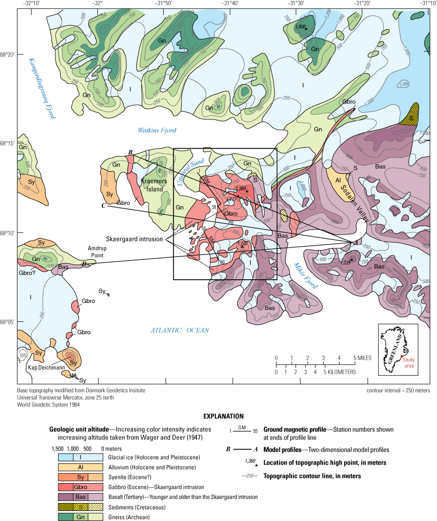
Generalized geologic map of the Skaergaard area, East Greenland, modified from Wager and Deer (1947). Ground magnetic profiles (GM) are also shown with identifying station numbers from the data release (Gettings and Parks, 2025) at the beginning, offset, and ends. Black box indicates the area shown in figure 2.
In addition to the layered rocks grouped into the lower, middle, and upper zones that make up the bulk of the intrusion, a marginal border group including the chilled margin that is up to several hundred meters thick and an upper border group are mapped (fig. 2). On the east side a younger, thick gabbro dike, named the Macrodyke (M, fig. 2), intrudes a short distance into the east side of the Skaergaard intrusion but is believed to continue beneath part or all of the Skaergaard (McBirney, 1996). A picrite body older than the Skaergaard intrusion is mapped to the north of the intrusion (P on fig. 2), as well as several older and younger gabbro dikes and sills in the surrounding terrane are not a part of the Skaergaard intrusion (McBirney, 1996). Subsequent to its solidification, a number of thin basaltic dikes intruded the Skaergaard gabbro and the surrounding host rocks. These dikes are related to the flexuring of the area (Wager and Brown, 1967). Figure 3 shows a cross section (profile A–A′) from north to south across the intrusion. The dolerite Basistoppen sheet intrudes the southern part of the Skaergaard intrusion beneath the upper border group (fig. 3) (Wager and Brown, 1967).
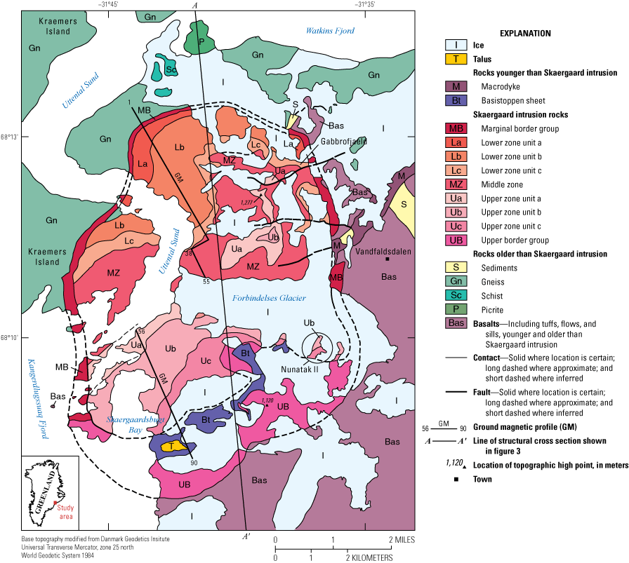
Geologic sketch map of the Skaergaard intrusion, East Greenland, modified from Gettings (1976) and McBirney (1996). Extent of figure 2 shown as inset box in figure 1.
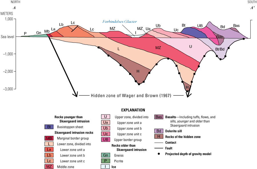
Schematic cross section of the profile A–A′ of figure 2 showing geologic contacts above sea level (modified from McBirney [1996]). The final gravity model from this report of the dike-like portion of the intrusion below sea level is shown added to the profile. The entire section has been tilted in a broad flexure to the southeast from about 10° in the northern part of the intrusion to 30° in the Tertiary volcanic rocks south of the intrusion (Wager and Brown, 1967).
The data collection and processing followed by the results of the modeling of the gravity and aeromagnetic data are described below. Both two-dimensional (2D) and three-dimensional (3D) modeling of the gravity anomaly map and 3D modeling of the aeromagnetic data were carried out using models that incorporated the dipping layering of the intrusion. These models required derivation and coding of computer programs for cylinders and polygonal layers that are dipping relative to horizontal. All computations except for the presentation of the gravity and aeromagnetic anomaly maps as shaded relief images were carried out with an IBM 360/50 at the University of Oregon Computing Center during the period 1971–1973. Computer input at that time was by decks of punched cards, and output was punched cards and printed paper. Only some of the computer printouts were extant at the time of the writing of this report. These datasets have not been superseded by publicly available modern data and are available in the accompanying data release by Gettings and Parks (2025).
Data Surveys
Gravity Survey
The Skaergaard gravity survey field work was completed in the period from July 24 to August 16, 1971, by H.R. Blank and M.E. Gettings using LaCoste-Romberg G-series gravimeter G-141 and Worden Master gravimeter W533. A total of 168 stations were established, of which 82 had altitudes determined by altimetry and 86 had known altitudes, mainly at approximate sea level determined by visual observation on the shoreline. Horizontal locations were recorded by labeled pinpricks on the 9″×9″ stereo aerial photographs. One day of helicopter use enabled us to obtain stations on several of the high, rugged basalt peaks east and south of the intrusion and Gabbrofjaeld (peak 1360, fig. 1). Approximately 14 traverses by foot, several including fly camps for two or three days were carried out, and at least 9 boat traverses were done. Several boat traverses were carried out with a motorized lifeboat and a rowboat. The expedition ship, the Signalhorne, was used for transport to and from various foot traverses and across Kangerdlugssuaq Fjord to Amdrup Point and Kap Deichmann. Watkins Fjord was obstructed by ice during the expedition and no stations could be established on the north shore. The captain of the Signalhorne plotted depth soundings on a map throughout the expedition to provide data on water depths along the coastlines, Kangerdlugssuaq and Mikis Fjords, and in Uttental Sund. Gravity station locations were compiled on a 1:50,000-scale base map (described herein) by scaling from features that could be located on both the aerial photographs and the base map. The only topographic map available at the time was the 1:250,000-scale map sheet Gronland 68.0.3 Kangerdlugssuaq of the Danmark Geodaetisk Institut (1969). This map was made from trimetrogon aerial photography taken by the United States Army Map Service (AMS) in the period immediately after World War II, coupled with ground control from surveys in 1933–34 and place names from 1955 expeditions. The base map was made from a photographic enlargement of the map sheet to 1:50,000-scale for an area 43 km east-west by 38 km north-south centered on the Skaergaard intrusion. The AMS trimetrogon aerial photographs, consisting of a right and left side-looking oblique photograph and a vertical photograph with stereo overlap, were obtained and used in the field for station locations. The resulting station distribution is 1 gravity station per 4 square kilometers (km2).
The gravity survey data were processed during 1971–1972 by M.E. Gettings and H.R. Blank, with some help from students in the digitization of 1:250,000-scale topographic maps for terrain corrections. It should be noted that the observed gravity values are on an arbitrary datum based on the reading of LaCoste-Romberg gravimeter G-141 on a base station upon return to the United States with no drift control. Drift of both gravimeters was computed using assumed linear drift between closures on the Skaergaard base station or temporary bases such as when working in the Mikis Fjord–Sodalen Valley area. Altitudes were determined by altimetry except those stations at or near sea level that were determined by Brunton compass leveling. Considerable effort was put into processing the altimeter data to obtain the best possible estimates of altitude. Given large barometric pressure variations due to changing weather conditions, most altimeter stations employed two or three altimeters so that a better estimate could be obtained. The correction scheme outlined in appendix 1 was used. Additionally, the barometric pressure records at three-hour intervals from the Danish weather station on the island of Nordre Aputateq, about 45 km south-southwest of the Skaergaard area, were obtained, which enabled reasonably good barometric corrections. After all corrections, the distribution of maximum difference between altimeters at the stations is shown in figure 4. The quantiles for these differences were (in feet [ft]) 0 percent, 0; 25 percent, 9; 50 percent, 18; 75 percent, 27; and 100 percent, 79, suggesting that about half of the altimetric altitudes are accurate to about ±10 ft.
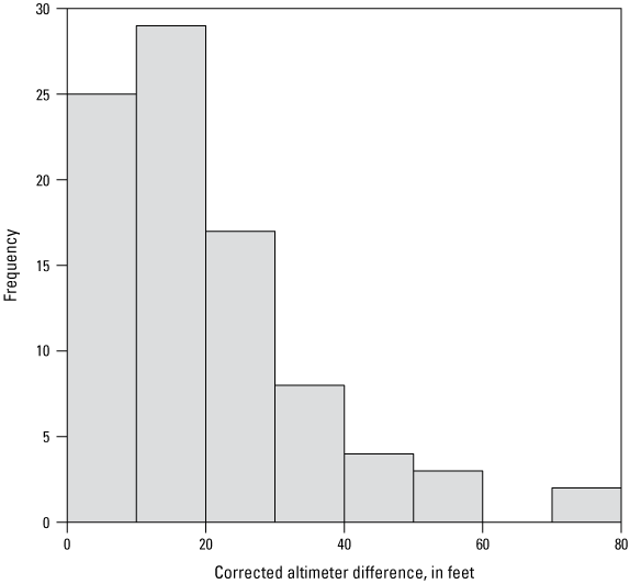
Histogram showing the maximum difference in feet in corrected altitude from the pairs or triplets of altimeters at gravity stations not at sea level or other known altitude, Skaergaard intrusion area, East Greenland.
Terrain corrections were carried out in four parts. The available 1:250,000-scale topographic maps were digitized using a grid of 1′ latitude by 2′ longitude for the survey area and at 3′ by 6′ intervals out to 167 km beyond the survey area with the estimated centroid altitude. Because bathymetric data were not available, the digitization was done at the ice altitude and sea surface. The Hayford-Bowie scheme of zone radii was used (Swick, 1942; Hayford and Bowie, 1912). The outer zone corrections from 2.29 km to 21.0 km were done using the 1′×2′ digitization, and corrections from 21.0 km to 166.7 km using the 3′×6′ digitization were computed using the program by Plouff (1977). The corrections for all stations from 68 m to 2.29 km were computed by transparent template over the 50,000-scale topographic map by H.R. Blank. The innermost corrections from the station to a radius of 68 meters (m) were computed by M.E. Gettings from the field notes using a combination of Hayford-Bowie quadrants and displaced half-slopes. Finally, the 1′×2′ prisms were given average density values based on the geologic map (Wager and Brown, 1967) and the measured densities of hand specimens described below, and corrections to the usual constant density terrain corrections were computed. Figure 5 shows the frequency distribution for the final terrain corrections. The quantiles for the terrain corrections were (in milligals [mGal]) 0 percent, -1.3; 25 percent, 3.2; 50 percent, 5.7; 75 percent, 8.9; and 100 percent, 37.5. The lack of topographic maps at scales larger than 1:250,000 meant that the inner zone terrain corrections, especially the Hayford-Bowie A–F zone (0–2.29 km about the station), have a large possible error. Given this, the error envelope for the terrain corrections is probably about ±20 percent. Thus, the error for half of the stations is about ±1.2 mGal or less, with larger uncertainties for stations with larger corrections.
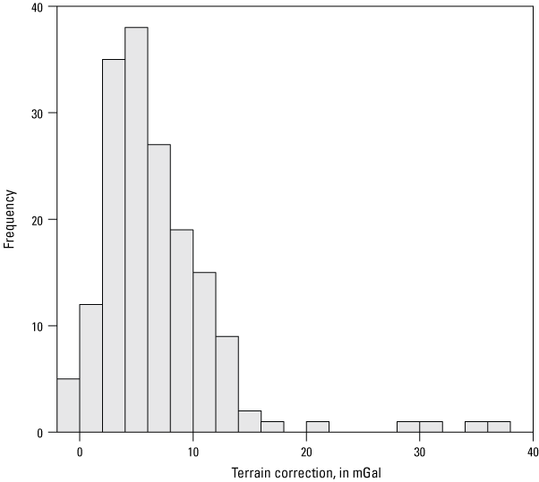
Histogram showing the frequencies of the total terrain correction in milligals (mGal) for the variable Bouguer gravity reduction, Skaergaard area, East Greenland.
As previously noted, the terrain corrections were carried out with data digitized to the ice altitude and sea surface because there was no bathymetric or ice thickness data. To evaluate the uncertainty introduced by this, several computational experiments were carried out. A cross section consisting of a portion of an ellipse terminated by a horizontal plane (see appendix 2) was chosen as a model of glacial valleys (fig. 6) and was used to estimate glacier thicknesses and fjord depths. Figure 7 compares the elliptic fit with soundings taken by the expedition ship on a traverse across Kangerdlugssuaq Fjord. For glacier profile estimates, the seaward part of young glacial Sodalen Valley (location in fig. 1) is bedrock, and a topographic profile across it from the base map was used to define the parameters.
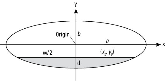
Diagram showing geometry for fitting a part of an ellipse of width (w) to approximate the geometry of the subsea or sub-ice area beneath a fjord or ice-filled valley of depth (d). The parameters a and b are the ellipse semi-major and semi-minor axes, respectively, truncated by a horizontal plane top.
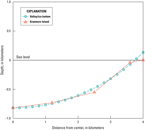
Plot comparing predicted depth to valley ice bottom based on an ellipse with 7.5-kilometer (km) width, 820 meters (m) depth at its center, and slope of 0.5 at the edge. Soundings were taken by ship crossing the Kangerdlugssuaq Fjord from Amdrup Point to Kraemers Island. Plot is from Kangerdlugssuaq Fjord center to Kraemers Island, East Greenland. For formulae used in calculations, refer to appendix 2.
Corbató (1964) derived the expression for the gravity effect of a 2D model using a cross section with a vertical axis parabola for the base truncated by a horizontal line for the top, and Corbató (1965) applied it to a glacier in Washington State where drill hole depths were available. M.E. Gettings compared this model to the similar model of a cross section with a portion of an ellipse and concluded the ellipse was a better representation as it gives a better fit to the increasing curvature at the model edges, even though the ellipse model case requires numerical integration. Using the width-to-depth ratios and slope at the edge from the Sodalen Valley profile (0.125 and 0.465), the ellipse semi-major and semi-minor axes were computed from the formulae in appendix 2, and then the gravity effect was computed from the formulae in appendix 3 for a range of glacier widths from 0.25 to 5.00 km. The results are summarized in figure 8 for a gravity station on bedrock at the edge of the glacier and for a station 100 m away from the edge on bedrock. Almost all the glaciers with stations near their edge in the survey were less than a kilometer in width, so the error in not correcting for the ice is between −0.2 and −2 mGal. The fjords have a greater effect as they are generally much wider; however, the big fjords are 5 or more km distant from the intrusion except on the southwest and had an approximately constant effect that did not greatly affect the residual anomaly due to the intrusion. On the southwest, the water is fairly shallow (reaching 200 m depth 1–2 km offshore), and in Uttental Sund along the west margin of the intrusion, maximum depths are 50 m or less except for a narrow 100 m depth in the southern part opposite Forbindelses Glacier (Forbindelsesgletscher), so the error in the gravity anomaly is not large and is almost systematic because of its location along the west side of the intrusion. The effect of correcting for the water areas would be to increase the residual anomaly somewhat because the maximum residual anomaly (discussed in the “Gravity Survey Analysis” section) falls in part along southern Uttental Sund and Skaergaardsbugt (the peninsula south of Uttental Sund, fig. 2). The maximum effect from the water is estimated to be 1.5 mGal.
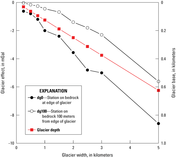
Graph showing the gravity effects in milligals (mGal) of a glacier model of elliptic base and horizontal top using parameters derived from Sodalen Valley (fig. 1) bedrock profile taken near the south end of the valley, Skaergaard intrusion area, East Greenland.
Standard Bouguer gravity anomaly reduction formulae were used to compute the Bouguer gravity anomaly at reduction densities of 2.67 and 2.77 grams per cubic centimeter (g/cm3). Although the median density for the measured hand specimens of gneiss is 2.675 g/cm3 (refer to table 1) a higher density of 2.77 g/cm3 was used because the gneiss contains numerous mafic dikes and gabbro bodies to the north and west of the Skaergaard intrusion. East and south of the intrusion it is bordered by gneiss overlain by basalt that has a median density of 2.95 g/cm3. The resulting anomaly map was still strongly influenced by the dense basalts and gabbros to the east and south, and because an interpretation objective was to use the software of Cordell and Henderson (1968) from sea level downward, it was decided to model all terrain above sea level in the gravity reduction. This is known as a variable density Bouguer gravity reduction (Vajk, 1956; Grant and Elsaharty, 1962; Gimlett, 1964).
Table 1.
Frequency distribution quartiles of measured whole-rock wet bulk densities for rocks of the Skaergaard intrusion and host rocks, East Greenland.[Consult McBirney (1996) for a discussion of trough bands (UTB) that occur in the upper zone. The Tinden sill is a granophyre that intrudes the upper border group (McBirney, 1996). Density values are grams per cubic centimeter (g/cm3). Abbreviations: %, percentile; No., number of samples; MB, marginal border group; UB, upper border group; L a, L b, and L c, lower zone units a, b, and c; M Z, middle zone; U a, U b, U c, upper zone units a, b, and c; GRV, granophyre; T S, Tinden sill; G n, gneiss; S y, syenite; B t, Basistoppen sheet; S, sediments; B a s, basalt; DIKB, basalt dikes]
The variable density reduction was accomplished in several steps. A program allowing different densities for each prism was coded similar to that of Plouff (1977) for the inner zone corrections (out to 15 km about the station) using the vertical line element prism formula outside of 2.29 km from the station but with density specified for each prism and a circular cylinder with specified density inside the 2.29 km radius. Using the geologic map (Wager and Brown, 1967) to determine rock unit, density data were measured from the 238 hand specimens and the 38 published in Wager and Deer (1939), and the 200-m topographic contours, the equal mass elevation and density contrast from 2.77 g/cm3 was estimated for each of the 1′ latitude by 2′ longitude prisms (fig. 9) within 15 km of stations. The hand terrain corrections (0–2.29 km about the station) were multiplied by the ratio of the density estimated at the station divided by 2.77 g/cm3. Repeating the hand terrain corrections on a variable density map was investigated for two stations in rugged basalt topography, and the difference from the ratio correction was in the hundredths mGal, so it was decided not to recalculate the hand corrections with the variable density template. The resulting gravity anomaly values thus have been corrected for the geology above sea level and reflect density variation from sources below sea level. The final corrected station gravity anomaly values were used to generate a grid using 1/r2 interpolation factor for surrounding stations where r is the distance from the grid intersection to the gravity station. The grid had a 1 km × 1 km cell size with an arbitrarily chosen origin 12.20 km south and 7.05 km west of peak 1277 (fig. 1). Figure 10 shows the final variable density Bouguer gravity anomaly map as a shaded relief image. This image used a new grid made using minimum curvature gridding techniques (Briggs, 1974) and was made using Oasis Montaj software (Geosoft, 2015). The variable density gravity anomaly map of the Skaergaard and its local surrounding area was originally published in Gettings (1976).
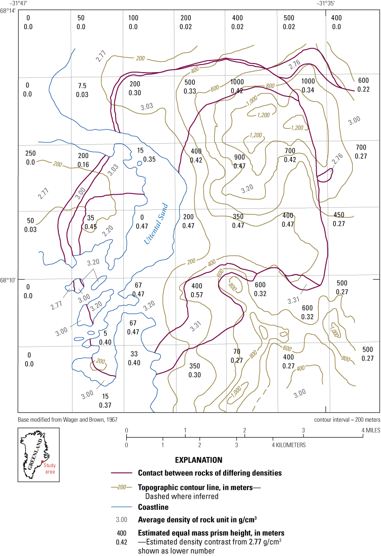
Gravity anomaly map showing the 1×2-minute prisms used to correct for the variable rock density above sea level, Skaergaard intrusion, East Greenland. Average density of the rock units given in grams per cubic centimeter (g/cm3).
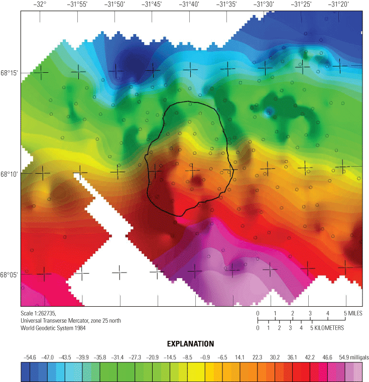
Variable density Bouguer gravity anomaly map overlain atop shaded relief base, Skaergaard intrusion, East Greenland. The gravitational effect of all terrain above sea level has been removed based on model density of figure 9. Station locations have been adjusted to the WGS84 datum. Refer to the accompanying data release (Gettings and Parks, 2025) for details. The observed gravity values are on an arbitrary datum based on the reading of LaCoste-Romberg gravimeter G-141 on a base station upon return to the United States with no drift control. Circle symbols are gravity station locations, and the approximate outline of the Skaergaard intrusion is shown in black.
Aeromagnetic Survey
The aeromagnetic survey was conducted on July 5–7, 1971, using a Varian proton precession magnetometer with sensor towed by a Beechcraft Twin Bonanza aircraft when the weather cleared for a 2.5-day period. Flights were conducted from Isafjordur, Iceland, the northwesternmost airstrip available with logistic support that was 450 km from the study area. The flight on July 5, 1971, was flown at 15,000 ft altitude to take vertical photographs using a Hasselblad camera that was used to plot and locate the tracking photographs from the magnetometer flights the following 2 days (changes in the glacier shapes and snow cover from the stereo photography meant that the low level photographs from the magnetometer flight could not be reliably located on the stereo photographs without first locating the higher altitude photographs on the stereo photographs). The magnetometer flights were flown at a barometric altitude of 5,000 ft on July 6 and 7, 1971. Nominal flight line spacing was 1 km and navigation was visual. Four north-south tie lines were flown, one near the east and one near the west edge of the survey area, and two were flown in the center about 2 km apart, both crossing the intrusion. The main survey was flown in twenty east-west flight lines, with two approximately 10-km north-south lines over the northern two thirds of the intrusion north to the Watkins Fjord shoreline. Tracking photographs were taken with 35mm cameras vertically through a port in the aircraft belly and magnetometer data were recorded on a strip chart recorder with time and navigation fiducial marks.
Diurnal variation was estimated using the records of the Leirvogur Magnetic Observatory in Iceland (lat 64.183° N., long 21.70° W.), the nearest station, 620 km to the southeast. Vertical tracking photographs from the aircraft were plotted on the Hasselblad photographs and then using the Hasselblad photographs the points were located and plotted on the 9″×9″ stereo photographs. Using the stereo photographs, the points were then compiled on a base map at 1:50,000 scale. Magnetometer readings from the magnetometer strip chart were measured and plotted at approximately 300- to -700-m intervals on the base map with an arbitrary datum of 53,000 nanoteslas (nT). Several corrections were applied to the magnetometer readings. One was the “recorder drift” amounting to ±0–15 nT. This was determined by periodically comparing annotations on the strip chart of the digital magnetometer display versus the value on the strip chart plot scale. Secondly, the intersections of tie lines with flight lines were used to scale and adjust the diurnal variation values determined from the observatory record. The recorder drift and final diurnal values (amounting to 40–65 nT on the 6 July 6, 1971, flight, and 9–16 nT on the July 7, 1971, flight) were subtracted to yield final magnetic anomaly values and annotated on the base map; the resulting map sheet was hand contoured. The map sheet with the annotated points is still available and has been digitized, rectified, and used to generate the aeromagnetic anomaly grid, so the bias from hand contouring has been avoided. A shaded relief map of the aeromagnetic anomaly is shown in figure 11.
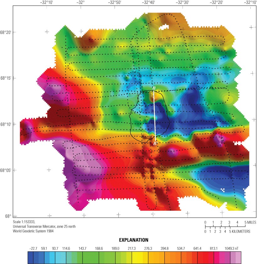
Aeromagnetic map of the Skaergaard area, East Greenland, showing flight lines (black dots). The approximate outline of the Skaergaard intrusion is shown as a black line, and the analyzed profile B–B′ is shown as a white line. Refer to the data release by Gettings and Parks (2025) for details. nT, nanotesla.
Ground Magnetic Profile
A ground magnetic profile of the vertical field component was carried out by H.R. Blank and M.E. Gettings during August 14–16, 1971. The instrument used was a Scintrex model MF-1-100 fluxgate magnetometer, serial number 809371. The unit and battery pack weighed 3.6 kilograms (kg) and was suspended on a harness in front of the operator. It was necessary for the operator to remove all metal from his person as belt buckles, pens, and so forth, would cause errors in the readings. Readings were taken from the galvanometer on the instrument and recorded to the nearest 5 nT. The ground magnetic profile began in the gneiss of the Uttental Plateau, crossed the marginal border group, all the zones of the layered series, and finished on the Basistoppen sheet (fig. 2), extending approximately 9,020 m in two segments. The location of the profile shown on figures 1 and 2 is approximate because precise station locations have been lost as they were pinpricked on the aerial photos that are no longer available. The interval between readings was approximately 100 m, determined by pacing. A large magnetic offset occurred at 0500 Norway Standard Time, shown by the record (fig. 12) from the Leirvogur Geomagnetic Observatory, Iceland. Because of the highly magnetic rocks of the Skaergaard intrusion, the offset was as much as +2,300 nT, then recovering with time. The drift curve of figure 12 was constructed using the reoccupations of base and some field stations together with the shape of the Leirvogur Observatory record, and the observed data were corrected using this drift curve.
The final corrected profile is shown in plots for the north and for the south segments, (figs. 13 and 14, respectively). In the southern segment, the re-occupations during the large offset can be seen between the 1,000 and 1,500 m distances and show that the drift was satisfactorily compensated for the purposes of this study.
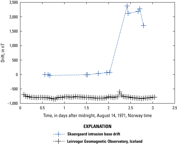
Graph of Skaergaard intrusion base drift used to correct ground magnetic profile data, East Greenland. nT, nanotesla.
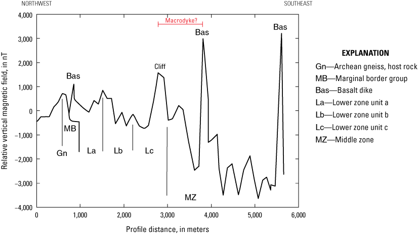
Graph showing northern segment of the final corrected ground magnetic profile across the Skaergaard intrusion, East Greenland. “Cliff” denotes observations along the base of a cliff with substantial magnetic rock above the magnetometer as well as below. The superposition of the Macrodyke may also be present in the northern segment of the ground magnetic profile (bracketed and labeled “Macrodyke?”). Refer to figure 2 for description of units and location of profile. nT, nanotesla.
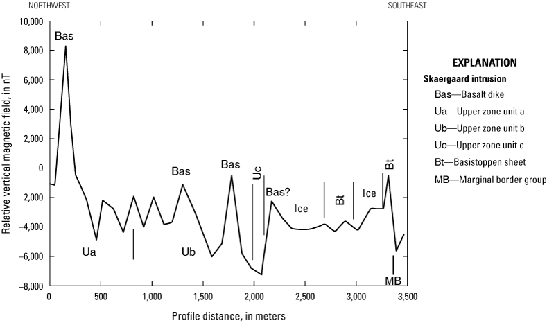
Graph showing southern segment of the final corrected ground magnetic profile across the Skaergaard intrusion, East Greenland. Triangular plot at approximately 1,300 meters (m) shows values at reoccupied stations corrected for large offset in the magnetic field on August 16, 1971, relative to August 15, 1971 (fig. 12). Refer to figure 2 for description of units and location of segment. nT, nanotesla.
Physical Property Data
Specimen Bulk Density
Bulk density determinations were carried out using the weight-in-air and weight-in-water method. Specimens were soaked in water at least overnight to fill any pores connected to the surface of the specimen. Repeat measurements with the apparatus used yielded a precision of ±0.005 g/cm3 or better for all specimens measured. The sample was weighed three times, together with measurement of the water temperature to obtain the necessary data for determining bulk and grain density,where
wair
weight of the specimen in dry air,
wwater
weight of the specimen saturated and immersed in water, and
wairwet
weight of the specimen saturated but surface dry in air.
Then the dry bulk density ρbd is given by
whereρwater
is the density of water at its temperature during the measurement (Jones and Harris, 1992).
The saturated (wet) bulk density ρbw is given by
The specimens measured were all non-porous so there was no significant difference in wet and dry bulk density. In the case of volcanic lavas, virtually all vesicles were filled with various zeolites and calcite so that the porosity was near zero. In addition to the 238 measured specimens, specific gravity measurements for 38 specimens reported in Wager and Deer (1939) were included in the dataset in the accompanying data release (Gettings and Parks, 2025). Table 1 gives the distribution of densities for the various lithologies and the units of the Skaergaard intrusion. Figure 15 shows a boxplot of the median densities for units of the Skaergaard and the host rocks. The median density for the gneiss is 2.675 g/cm3 and that of the basaltic lavas is 2.950 g/cm3. Since the northwest half of the intrusion host rock is gneiss (and presumably at depth beneath the basalts to the south) and the southeast half has basaltic lavas as host rock, a Bouguer gravity reduction density of 2.77 g/cm3 was chosen for reduction of the gravity survey data described.
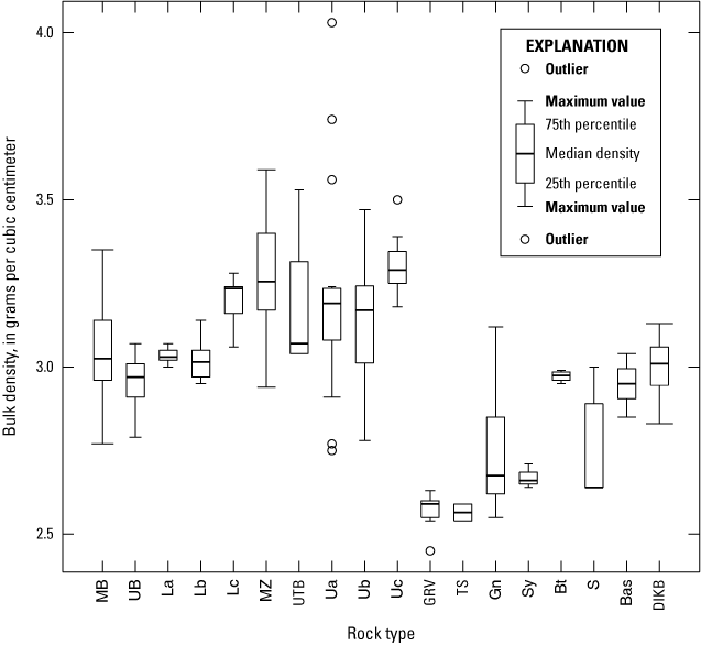
Boxplot of measured densities grouped by geologic unit from table 1 for the study region, Skaergaard intrusion and host rocks, East Greenland. Heavy line is median density, box is 25 and 75 percent quartiles, and maximum and minimum values shown as whiskers or points. If all points are within 1.5 times the interquartile range (75-percent quartile minus 25-percent quartile) from the median the whisker is the maximum or minimum. If some points are farther from the median, the whisker shows 1.5 times the interquartile range off the median, with points farther shown as circular symbols. MB, marginal border group; UB, upper border group; L a, L b, and L c, lower zone units a; b, and c; M Z, middle zone; UTB, upper zone trough bands; U a, U b, and U c, upper zone units a; b, and c; GRV, granophyre; T S, Tinden sill (a granophyre sill intruded in UB); G n, gneiss; S y, syenite; B t, Basistoppen sheet; S, sediments; B a s, basalt; DIKB, basalt dike.
Specimen Magnetization
Eighteen oriented specimens were collected of which fourteen were from the intrusion and four were from basalt dikes, the Basistoppen sheet, and a granophyre dike (table 2). These specimens were core-drilled and measured in a spinner magnetometer (Doell and Cox, 1965) located with the Geophysics Group at Oregon State University. No demagnetization was carried out because the demagnetizing instrument was broken. The magnetic susceptibility of the cores was measured with a susceptibility bridge, also available at Oregon State University. The resulting data were reduced to produce remanent magnetization directions and intensities using the algorithm given in Doell and Cox (1965). Table 2 reports the magnetization properties for these specimens and figures 16 and 17 show the reversed and normal remanent directions on stereographic plots. The normally polarized specimens have a Q (Koenigsberger ratio of remanent magnetic intensity to Earth field induced magnetic intensity, Grant and West, 1965) of 0.09 (granophyre) to 3.91 (basalt dike). With the exception of one specimen (HRB–7A, from the chilled margin in a disrupted zone at the northern intrusion contact), the intrusion specimens are all reversely polarized with an average inclination of −47.7°, declination of 187.2°, and average intensity of magnetization of .003 electromagnetic system of units per cubic centimeter, median 0.00316±0.00582. Median Q is 1.64±0.58 (interquartile range). This corresponds to an average susceptibility of 0.0034 centimeter-gram-second electromagnetic system of units (cgs) with the remanent 1.64 times this in the reversed direction. Subsequent to the work reported here, Schwarz and others (1979) reported their results of samples collected in 1976 using diamond drill sampling and including demagnetization analysis. Their results are an average inclination of −59°, declination of 170°, and they are likely more accurate than those reported here because of uncertainty introduced using oriented hand specimens rather than drilled cores.
Table 2.
Measured natural remanent magnetization and magnetic susceptibility of oriented specimens, Skaergaard intrusion, East Greenland.[All intrusion specimens are reversely polarized, except HRB–7A. Remnant magnetization directions and intensities were produced using the algorithm given in Doell and Cox (1965). Abbreviations: ID, sample identification number; I, inclination degrees positive downward from horizontal; D, declination degrees clockwise from north; Jrem, centimeter-gram-second electromagnetic system of units intensity (cgs), units of 10-3 electromagnetic system of units per cubic centimeters; K, cgs magnetic susceptibility, units of 10-6); Q, Koenigsberger ratio; CMGabbro, chilled margin gabbro; cm, centimeter; L a, lower zone unit a; m, meter; L b, lower zone unit b; L c, lower zone unit c; M Z, middle zone; Mt, magnetite; U b, upper zone unit b; U c, upper zone unit c; opx, orthopyroxene; aug, augite; RevAvg, average magnetization direction and intensity of all reversely magnetized samples; NA, not applicable; Is., island; NrmAvg, normal average]
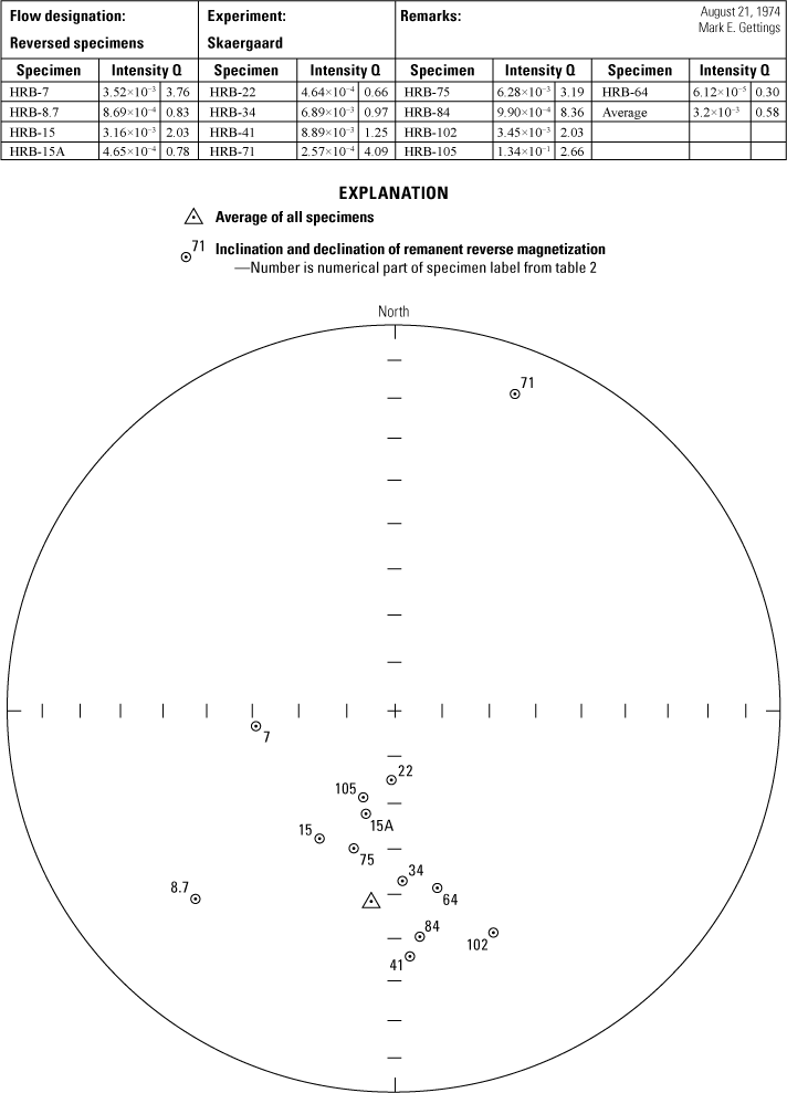
Stereographic plot of measured natural remanent magnetization directions for specimens that have reversed directions, Skaergaard intrusion, East Greenland. Approximate locations of the specimens are given in the data release (Gettings and Parks, 2025) for the ground profile.
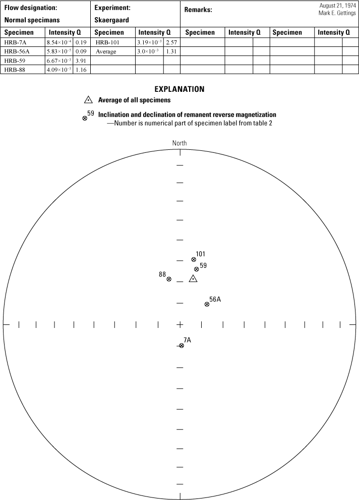
Stereographic plot of measured natural remanent magnetization directions for specimens that have normal directions, Skaergaard intrusion area, East Greenland. Approximate locations of the specimens are given in the data release (Gettings and Parks, 2025) for the ground profile.
Quantitative Interpretation
Gravity Survey Analysis
Based on geologic mapping and analysis of the differentiation trends (cryptic variation, Wager and Deer, 1939) of the rocks from the exposed zones and the chilled margin of the marginal border group, Wager and Deer (1939) predicted that the intrusion must include what they call a “hidden zone” amounting to 60 percent of the volume of the original intrusion. After further analysis, Wager and Brown (1967) estimated the hidden zone to be 70 percent of their original estimated volume of 500 cubic kilometers (km3) for the entire intrusion, giving a volume estimate for the hidden zone of 350 km3. The cross section given in Wager and Brown (1967) shows the hidden zone as a cylinder of about 7.5 km diameter at the base of the lower zone and narrowing to 5 km diameter at the bottom. Using an average diameter of 6.25 km and volume of 350 km3 this gives a height of 11.4 km for the cylinder. The continental margin flexure, which averages 22° down to the southeast across the intrusion, should make the hidden zone more nearly a vertical cylinder, judging from the cross section given in Wager and Brown (1967). Assuming the contact between the hidden zone and the lower zone to be approximately planar, the contact is at sea level at the northern end of the intrusion and at about 4 km depth at the southern end. The expected gravity anomaly on the axis of such a cylinder, computed from the formulae of Dobrin (1960) with a density contrast of 0.3 g/cm3 would be 30.6 mGal at 0 km depth (northern end of the intrusion), 17.0 mGal at 2 km depth (middle of the intrusion), and 9.6 mGal at 4 km depth (southern end of the intrusion). Calculating a horizontal profile for such a cylinder (Nabighian, 1962) gives an expected width of the anomaly at half amplitude (half width) of approximately 7 km. This estimate does not include the gravity effect of the exposed zones that are below sea level (fig. 3; also fig. 9 in Wager and Brown, 1967). Estimating this effect with half a cylinder of 4 km radius, density contrast of 0.42 g/cm3 (average of lower, middle, and upper zones) and 2-km thickness gives 13.4 mGal at the center of the intrusion; together with the 17.0 mGal from the hidden zone at the middle of the intrusion, the anticipated gravity effect from the Wager model of the intrusion below sea level is about 30 mGal.
A regional gravity anomaly trend surface was computed using orthogonal polynomials (Oldham and Sutherland, 1955) with a least-squares fitting program on the 1 km gravity anomaly grid to account for the large, approximately north-south gradient across the variable density Bouguer anomaly field (fig. 10). The program, originally written by Ron Wahl of the U.S. Geological Survey (USGS), is available as program “surfit” in Phillips (1997). Fits of first, second, third, fifth, seventh, and eighteenth order were examined. The coastal flexure gradient was judged best fit by the fifth order fit (fig. 18) and yielded a residual gravity anomaly map (fig. 19). This residual anomaly map was used for all interpretive modeling. The eighteenth order fit was examined to see if it made a suitable smoothed map but even at this high order too much of the shape and amplitude of the map anomalies were lost.
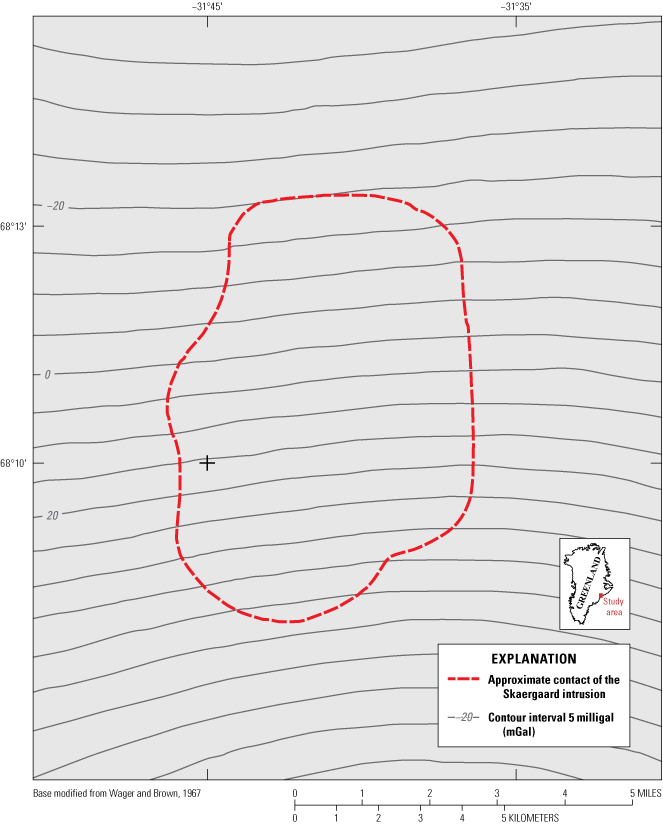
Fifth order orthogonal polynomial least squares fit (grid) to the variable density Bouguer gravity anomaly grid, Skaergaard area, East Greenland. Contour interval 5 milligals. The plus symbol near the western edge of the intrusion contact is lat 68°10′ N. and long 31°45′ W.
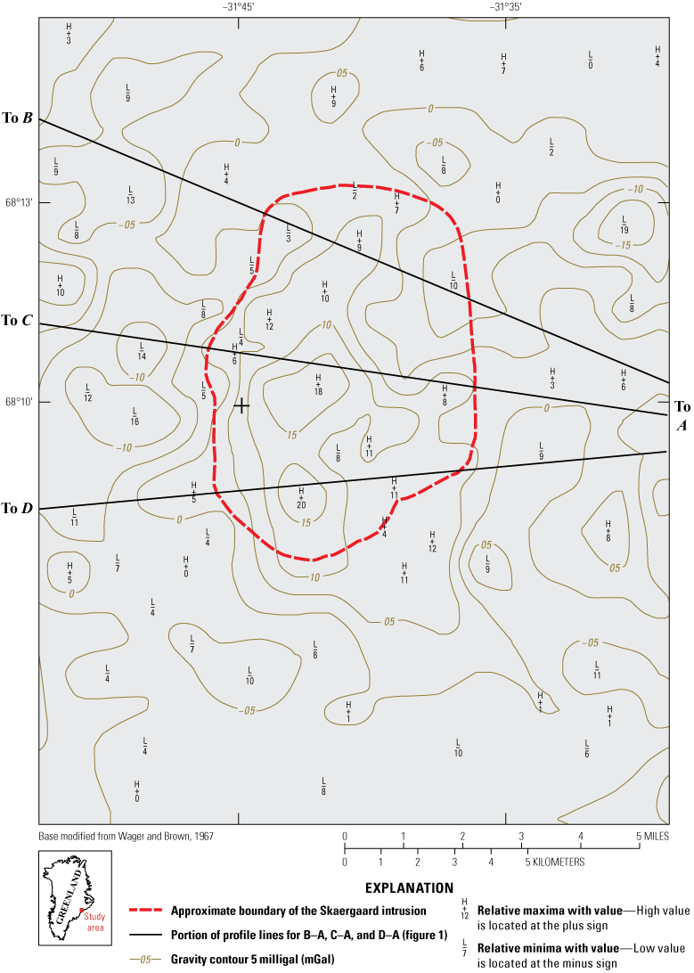
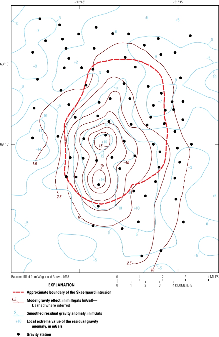
Residual gravity anomaly after subtraction of the fifth order polynomial fit grid from the variable density Bouguer gravity anomaly grid, Skaergaard area, East Greenland. Relative maxima (H) and minima (L) in the grid from the contouring program are shown with their value. Bathymetric depths were not included in the terrain corrections. The plus symbol near the western edge of the intrusion contact is lat 68°10′ N. and long 31°45′ W.
The residual gravity anomaly map (fig. 19) shows a north-trending, dike-like positive anomaly in the western part of the intrusion outcrop. The anomaly maximum varies from 7 mGal near the northern end to 20 mGal near the southern end of the intrusion, consistent with southward tilt and increasing volume of the intrusion below sea level. The half-width of the anomaly varies from 1.5 km in the north to approximately 3.5 km in the south-central portion to 2.5 km in the south. The maximum in the south occurs beneath the Basistoppen gabbro sheet (McBirney and others, 1989) which may contribute several mGal to the anomaly here and along the extent of the sheet in a northeasterly trend. To the east of the intrusion contact, a broad positive anomaly of approximately 5 mGal is probably due to a combination of the picrites in the Vandfaldsdalen area lava and gabbro including the Macrodyke (M in fig. 2) that cuts through the northern end of Vandfaldsdalen (McBirney and others, 1989). East of the intrusion’s northeast contact, the concentric low of −19 mGal and its extension to the southwest is likely due to the Haengfjeldet formation tuffs (McBirney and others, 1989) that were not accounted for by the variable density Bouguer reduction. The negative anomalies of −4 to −10 mGal to the southwest of the intrusion contact are due to seawater as bathymetric depths were not included in the terrain corrections. The anomaly lows and highs to the west and northwest of the intrusion contact are attributed to lithologic variations in the Precambrian metamorphic complex that contains both amphibolitic (dense) and quartzo-feldspathic (less dense) zones, as well as post-Skaergaard-age basaltic dikes and gabbro bodies (McBirney and others, 1989). Finally, the broad gravity anomaly high of 8 to 12 mGal to the south-southeast of the intrusion contact is due to picrite and dolerite sheets in the basaltic volcanic section (McBirney and others, 1989; Wager and Brown, 1967). The gravity anomaly due to the hidden zone of the intrusion and the below–sea level rocks of the lower, middle, and upper zones is thus assumed to be the dike-like anomaly with a 2–3.5 km half-width and maximum amplitude of 18 to 20 mGal. The possible errors in anomaly values from the various sources is probably about ±2 mGal, so the estimated anomaly maximum amplitude is likely 16 to 22 mGal.
Two-Dimensional Models
Gravity values along profiles A–B, A–C, and A–D (figs. 1 and 19), were chosen to cross the relative maxima in the middle and southern part of the intrusion, and to cross a representative part of the northern part of the intrusion. The values were digitized from contour intersections and maxima and minima from the residual gravity anomaly map (fig. 19) and then digitized at a 500 m interval. They were first modeled using an iterative profile modeling program implementing the method of Bott (1960). A density contrast of 0.27 g/cm3 was used for the inversions, assuming a bulk density of 3.0 g/cm3 for the hidden zone and assuming that it is equivalent to the marginal border group (Wager and Brown, 1967). The resulting causative bodies were 3–4 km width at sea level, narrowing to about 1 km at 3–4.1 km maximum model depth. Because of the southward dip of the intrusion, some of the sub-sea-level rocks are part of an exposed series of rocks that in general are denser. Increasing the density contrast results in models that are shallower in their depth extent.
To further evaluate the anomaly, the width of a dike extending from the surface to 4 km depth was estimated from the gravity anomaly at various horizontal distances along the profiles (Dobrin, 1960). Width estimates from the gravity anomaly at 0.5, 1.0, and 1.5 km from the maximum for the three profiles gave dike width estimates varying from 0.6 to 0.85 km. Using the north-south cross section (profile A–A’, fig. 2) of the intrusion (fig. 3), the intersections of the three profiles were located on the cross section and the depths of the zone boundaries were measured. Densities used were 2.73 g/cm3 for the gneiss country rock, 3.03 g/cm3 for the lower zone, and 3.20 g/cm3 for the middle and upper zones. Two densities of 3.0 and 3.2 g/cm3 were assumed for the hidden zone to bracket the range observed for the exposed zones. The models for each profile consisted of a stack of rectangular 2D prisms (computed using formulae from Talwani and others, 1959) with density contrasts from the listed densities and thicknesses from the cross section for the exposed zones. The models’ hidden zones were then made to have total thicknesses of 1, 2, 3, 4, or 5 km by adding a prism at the bottom representing the hidden zone. These models were calculated for prism widths of 1 and 2 km. Table 3 gives the resulting hidden zone thicknesses for the models that fit the observed profiles within ±2 mGal, the estimated error envelope.
Table 3.
Stacked two-dimensional rectangular prism models for the three profiles (A–B, A–C, and A–D) in figure 19 of the Skaergaard intrusion, East Greenland.[Larger location map of profile lines is shown in figure 1. The models for each profile consisted of a stack of horizontal rectangular two-dimensional prisms, computed using formulae from Talwani and others (1959). Table values are vertical thicknesses in kilometers (km) of the component prisms. Density is density contrast in grams per cubic centimeter (g/cm3) HZ values are the vertical thickness that produce models fitting the profile within the estimated error envelope of ±2 milligals. Abbreviations: UZ, upper zone; MZ, middle zone; LZ, lower zone; HZ1, hidden zone 1-km width prisms; HZ2, hidden zone 2-km width prisms]
The half-width of the 1 km width profiles was about 2 km, and for the 2 km width models it was about 3 km, suggesting, as in the Bott (1960) models, that the sub-sea level body is 2–3 km wide at the top and narrows to a km or less at depth. The largest hidden zone thickness possible is 4 km (table 3), using 1 km prisms and assuming profile A–C has a maximum value of 20 mGal (18 mGal observed plus 2 mGal error) and using the probable minimum density contrast for the hidden zone. These models support the conclusion that the sub-sea level part of the intrusion is probably less than 5 km in maximum depth.
Three-Dimensional Models
The excess mass (Grant and West, 1965) of the intrusion beneath sea level was calculated using a smoothed version of the residual gravity map over a 20×20 km area centered on the intrusion. The smoothed map removed the highs and lows outside the intrusion to reduce error. The integration was carried out using Simpson’s Rule (Abramowitz and Stegun, 1964) and the correction for finite integration area (Grant and West, 1965) was applied. Depending on whether one uses a horizontal cylinder or a sphere approximation to estimate the depth to center of mass, the estimated mass of the intrusion beneath sea level is 13.17×10¹⁵ to 13.58×10¹⁵ g. Because the intrusion is elongate in the north-south direction, choosing an intermediate value closer to the horizontal cylinder gives 13.3×10¹⁵ g as the best estimate.
Several 3D models were computed to further define the sub-sea level shape of the intrusion. First, the program of Cordell and Henderson (1968) was used to model the smoothed residual gravity anomaly grid iteratively with prisms beneath each grid point extending from sea level down to a depth such that the model fits the gravity grid. Two such models were computed, one with a prism density contrast of 0.3 g/cm3, a clear minimum considering the sub-sea level middle and upper zone rocks, and 0.4 g/cm3, a better estimate of the sub-sea level intrusion average density contrast. The 0.3 g/cm3 model is published in McBirney (1996) as a contour map figure. This model has two maximum depths of 3.7 km beneath the central maximum and 3.8 km beneath the southern maximum. The 0.4 g/cm3 model is probably more realistic, at least in the southern half, and has maximum depths of 2.7 and 3.0 km (fig. 20) and is the best estimate of the sub-sea level part of the intrusion using this method.
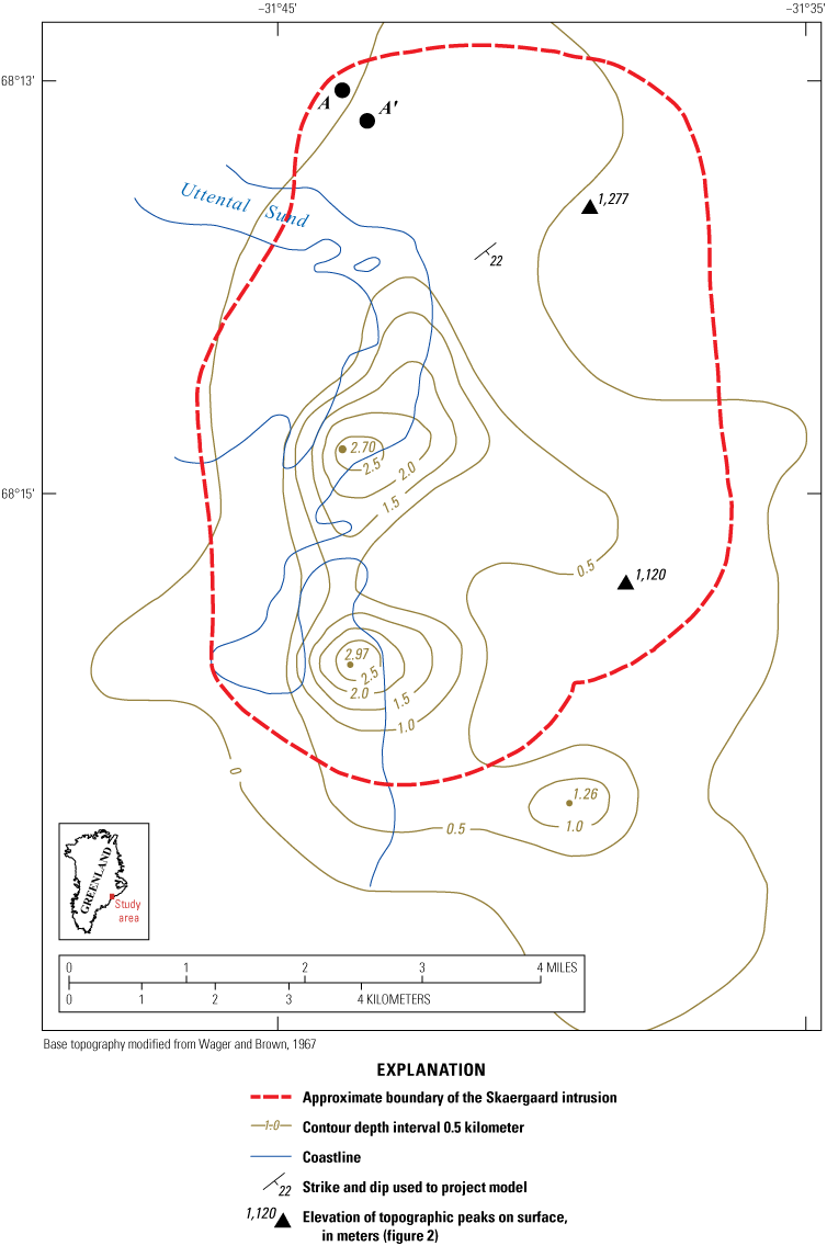
Contour map of the depth below sea level of the Skaergaard intrusion, East Greenland, using the iterative technique of Cordell and Henderson (1968) with the smoothed residual gravity anomaly after removal of a fifth-order polynomial fit from the observed gravity anomaly and a constant density contrast of 0.4 grams per cubic centimeter. Depths are in kilometers. Also shown is the average strike (55° clockwise from north) and 22° southeast dip used to project this model to contours on a dipping plane. Point A is the location of the lowest stratigraphic outcrop of the lower zone rocks, and A′ is its projected location. Points 1277 and 1120 are topographic peaks on the surface (figs. 1 and 2) used to establish a latitude-longitude grid on the geologic map of Wager and Brown (1967). Uttental Sund shoreline in blue; approximate contact of the Skaergaard intrusion in dashed red.
To make a more realistic model than one with a constant density contrast, the polygonal layer model of Talwani and Ewing (1960) was considered. This model is designed for horizontal layers that would require complicated estimates of the density contrast that would be applied to the Skaergaard intrusion, given its southward tilt. Instead, a more appropriate model is one with dipping polygonal layers of constant density contrast that simulates the average dip and strike of the intrusion zones. To do this, the horizontal components of the gravitational attraction of a polygonal layer were derived by the author using the computer code of Talwani and Ewing (1960) modified to calculate the vector components. Then the gravity effect (vertical component of attraction) of a dipping layer could be obtained by a simple coordinate transformation applied to the gravitational attraction vector for the dipping layer. Examination of geologic map relations (Wager and Brown, 1967) indicates the zones have an average strike of N.55° E. and average dip of 22° SE. The calculated grid of the Cordell and Henderson (1968) model depths (fig. 20) was projected to this plane, and the contours of equal depth in the dipping coordinate system were used to define the polygons for the zones. Density contrasts for the zones were: overlying basalts, upper border group, and Basistoppen sheet, 0.27 g/cm3; upper zone, 0.50 g/cm3; middle zone, 0.47 g/cm3; and lower zone and hidden zone, 0.27 g/cm3. In all, 31 layers were used in the model. The coordinates of the 82 gravity stations in the intrusion and immediate surroundings were also projected so that the model was calculated at the actual altitudes and locations of the stations as opposed to the Cordell and Henderson model that is calculated on a sea-level plane. This is important because most of the stations in the central and eastern part of the intrusion are at high altitudes whereas the stations of the western part of the intrusion are at or near sea level. Figure 21 shows the projected, dipping contour map of the model in figure 20. Figure 22 is a contour map of the final dipping polygonal-layer model gravity effect, including the smoothed residual gravity anomaly from figure 19 for comparison. This model fits the residual gravity anomaly within ±2 mGal in the area within a 1 km buffer about the intrusion contact except in the southeast where dolerite sills in the basalts were not modelled. The mean misfit at the stations is −1.4 mGal and the root-mean-square misfit is 3.67 mGal, due to the negative anomalies in the gneiss to the west and the sediments/tuffs to the northeast. Within a 1 km buffer around the intrusion contact, the mean misfit is −0.65 mGal with a root-mean-square misfit of 3.0 mgGal. The density contrasts could be changed slightly for one or more layers to improve the fit. However, since the fit was well within the ±2 mGal estimated error envelope, no further models were computed.
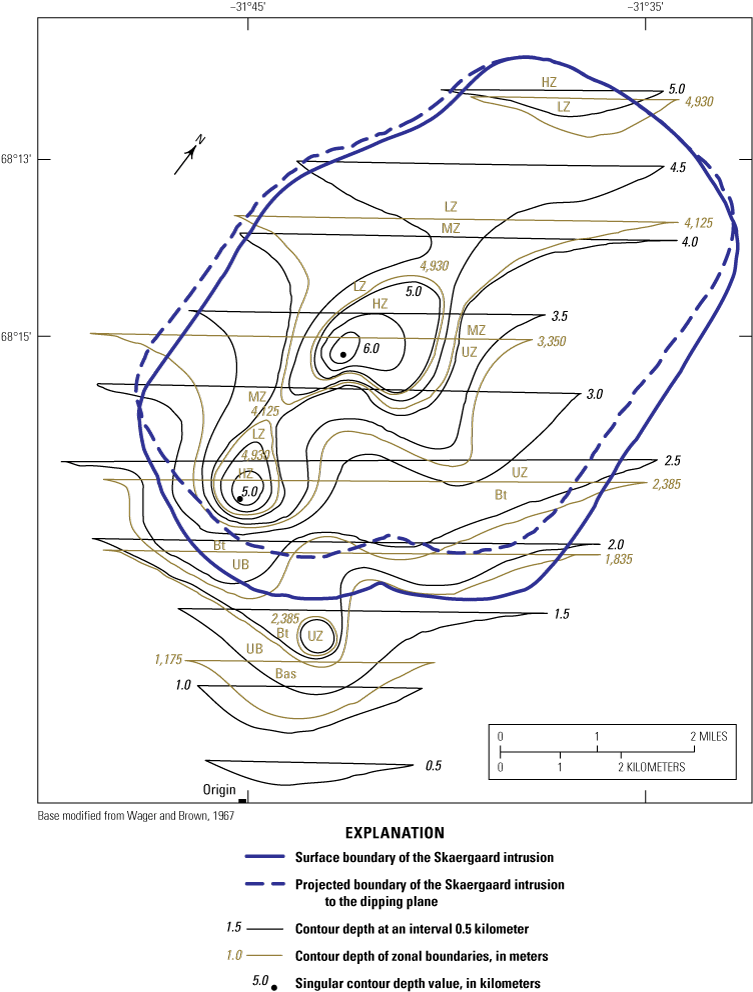
Contour map of the model in figure 20 of equal depths from the arbitrary origin (point labeled “origin”) perpendicular to a plane of strike 55° clockwise from north and 22° southeast dip, used to generate the layers of the dipping polygonal layered gravity model (fig. 22), Skaergaard intrusion, Greenland, East. The horizontal parts of the contours are at sea level. Zonal boundaries are abbreviated: hidden zone (HZ), lower (LZ), middle (MZ), upper (UZ), upper border group (UB), Basistoppen sheet (Bt), and basalt dolerite sill (Bas).
Model gravity effect of the polygonal layered model shown in figure 21. The polygonal layers dip at 22° to southeast with strike 55° clockwise from north. Layers have density contrasts representative of the Skaergaard intrusion zones extending below sea level.
Because further understanding of the crystallization and differentiation sequence of the intrusion was a primary objective of the research effort, the final calculations were to estimate crudely the relative volumes of the various zones. Subsequent erosion of the intrusion and surrounding host rocks preclude determination of the original extents of the zones, so a tilted-right elliptical cylinder truncated by the horizontal plane of sea level was used as a model for the above–sea level part of the intrusion (fig. 23). This seemed a reasonable model since it is unknown whether the original zones were larger or smaller than a cylindrical model. A best-fitting ellipse was calculated fitting the projection of the intrusion margin dipping at 22° southeast with strike N. 55° E., resulting in a cross-sectional area of 54 km2. Appendix 4 details the calculation of the volume of the wedge-shaped portion of the elliptic cylinder. Below sea level, the polygonal layered model discussed above together with the average densities was used to calculate the zonal volumes and excess masses relative to the gneiss density of 2.73 g/cm3. Layer volumes were calculated using the formula for polygonal area (Harris and Stöcker, 1998) for each lamina and then numerically integrated across the thickness of the zone. Figure 23 shows the results of these computations; it is notable that the estimated volume of the hidden zone is only about 1 percent of the intrusion volume.
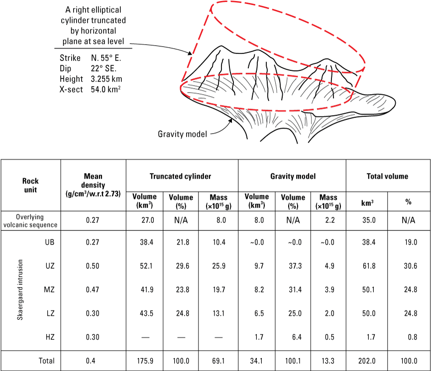
Diagram of best-fitting ellipse for the projection (A) of the intrusion margin with a strike of N. 55° E. and dipping 22° SE., and tabulated final estimated volumes and corresponding excess masses (B) of the Skaergaard intrusion relative to the gneiss country rock. Volumes are based on a truncated, tilted-right cylinder of elliptic cross section for the portion above sea level (maximum height 3.255 kilometers [km]) and dike-like structure based on the gravity model (fig. 20) below sea level. X-sect, cross-sectional area; km2, square kilometers; g/cm3, grams per cubic centimeter; w.r.t, with respect to; km3, cubic kilometers; %, percent; g, gram; N/A, not applicable; UB, upper border group; ~, approximately; UZ, upper zone; MZ, middle zone; LZ, lower zone; HZ, hidden zone;—, no data.
Three-Dimensional Modeling of Aeromagnetic Data
Interpretation of the aeromagnetic map was focused on the Skaergaard intrusion, although study of the map (fig. 11) shows significant structural boundaries trending approximately east-west across the map area. In part, these boundaries are related to rock units of reverse and normal magnetization, especially the intrusion and the older basalts to the east being reversely polarized against the normally polarized, younger basaltic section to the south, but there are also significant east-west magnetic boundaries to the north in the Watkins Fjord and gneiss terrane (figs. 1 and 2). Across Kangerdlugssuaq Fjord to the west (fig. 1), the Kangerdlugssuaq complex and Kap Edvard Holm intrusive complex 10-15 km southwest of the Skaergaard intrusion (Wager and Brown, 1967) have positive anomalies and so appear to be normally polarized. Within the Skaergaard intrusion the normally polarized Macrodyke (unit M in fig. 2) appears to persist as a positive anomaly that reduces the total amplitude negative anomaly from the Skaergaard intrusion approximately east-west across the intrusion in the subsurface into Kraemers Island (fig. 11). Several faults mapped within and around the intrusion (McBirney and others, 1989) may be correlated with some horizontal gradients on the aeromagnetic map.
The quantitative interpretation was carried out in early 1972, before the 3D Talwani-style polygonal layer software was available. Instead, the author had completed generalizing the right circular cylinder model of Reilly (1969) for an arbitrarily oriented cylinder, rather than one with a vertical axis, and this was used to model a profile across the intrusion. The profile B–B′ was chosen along a north-south line over the highest topography (fig. 11) to obtain the best signal-to-noise ratio at the constant flight height of 1,500 m (5,000 ft). The profile data were taken at 500 m intervals from the aeromagnetic anomaly map and carefully checked against the flight line strip charts to obtain the best estimate of diurnal variation and guard against contouring errors. A linear increasing southward drift of 118 nT was removed from the profile. The resulting magnetic variations (circular symbols in figure 24) were modeled using dipping cylindrical slabs. Radii and centers of circular cylinders approximating the topography and intrusion zones were determined using the topographic map and geologic map of Wager and Brown (1967) and are shown in plan view in figure 25. To approximate the dip of the intrusion zones, the axes of all the cylinders dip at 22° to the southeast, so the circles shown in the plan view are actually somewhat elliptical. In all, 17 cylinders were included in the model, however the layers below the base of the lower zone (base of cylinder 12, fig. 25) only contributed a smooth, long-wavelength offset to the model and do not contribute to the profile model shape at lengths of 10 km and less. Figure 26 shows a cross section of the cylinders model along the profile. Cylinder 16 extended the hidden zone to 5 km depth and cylinder 17 extended the hidden zone of Wager and Brown (1967) down to 20 km depths they proposed. Cylinders 16 and 17 do not contribute significantly to the model which is dominated by the magnetite-rich middle and upper zones. The large contributions of the middle and upper zones make it difficult to define any anomaly due to the hidden zone.
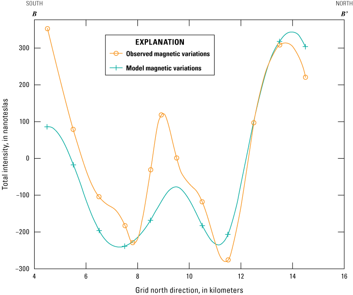
Graph of observed magnetic intensity and least squares fit of modeled intensity that is based on a dipping-cylinders model of the aeromagnetic data along the south-north profile B–B′ shown on figure 11, Skaergaard intrusion, East Greenland.
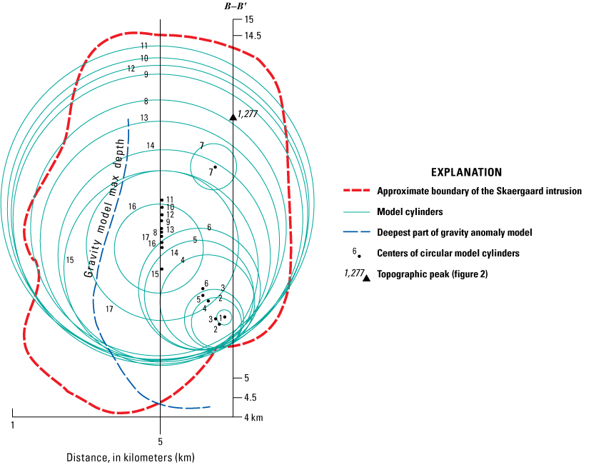
Map view of circular cylinder models of the aeromagnetic profile B–B′ with varying magnetic parameters appropriate for the zones of the Skaergaard intrusion, East Greenland. Note that the circles are only schematic as the cylinders dip 22° to the southeast with a strike 55° clockwise from north. Point 1277 is a topographic peak (fig. 1) the profile B–B′ crossed.
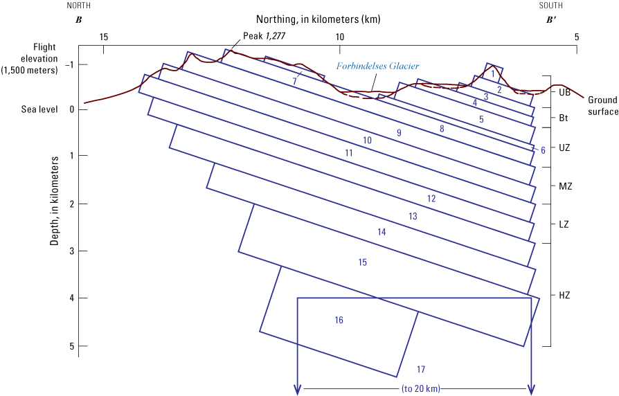
Cross section of the dipping circular cylinder model section of figure 25 along the aeromagnetic profile B–B′ with varying magnetic parameters appropriate for the zones of the Skaergaard intrusion, East Greenland. UB, upper border group; Bt, Basistoppen sheet; UZ, upper zone; MZ, middle zone; LZ, lower zone; HZ, hidden zone.
The geomagnetic induction field at the Skaergaard intrusion at the time of survey (July–August 1971) had a declination of 325°, an inclination of 79° downward, and an intensity of 53,500 nT (International Association of Geomagnetism and Aeronomy [IAGA], 2020). The relative magnetite contents of the zones were estimated using the Cross, Iddings, Pirsson, Washington (CIPW) norms (a standard petrologic method to calculate the mineral composition from the bulk chemical analysis, Barth, 1962) from the average zone compositions given in Wager and Brown (1967). These magnetization estimates were combined with the induction vector and the remanent direction from the measurements given above to arrive at an effective magnetization vector of declination 145° and inclination 65° upward. The resulting effective susceptibilities (cgs units) were: upper border group, 0.008; Basistoppen sheet, 0.006; upper zone, 0.010; middle zone, 0.009; lower zone, 0.005; and hidden zone, 0.002. The hidden zone value was calculated from the CIPW norm of the proposed hidden zone composition given in Wager and Brown (1967). Note that these estimates are relative and can be scaled up or down as a group to fit the observed magnetic profile. The upper and middle zones contribute the main part of the model anomaly with lesser contributions from the other zones, as clearly shown on the northern and southern ground magnetic profiles (figs. 13 and 14). The least squares fit of the cylinder model to the observed profile is shown in figure 24 with the plus symbols. Note that the model does not include any contribution from the normally polarized dolerite sill on the south margin of the intrusion (grid north direction 4.5) which would increase the model response between 4.5 and 7.5 grid north direction, and the sharp relative positive peak in the middle profile is inferred to be the superposition of the Macrodyke in the shallow subsurface beneath the profile. The superposition of the Macrodyke may also be present in the northern segment of the ground magnetic profile (fig. 13) between profile distances 2,800 and 4,000 m because magnetite appears as a cumulus phase in large quantities in lower zone C and the middle zone (Wager and Brown, 1967) and would be expected to yield a more negative anomaly. It was concluded that the exposed rocks of the intrusion and their subsurface extent account for essentially the entire aeromagnetic anomaly and further modeling was not attempted.
Conclusion
The gravity survey of the Skaergaard intrusion after correction for density and extent of the rocks above sea level resulted in a relatively narrow north-trending residual gravity anomaly of dike-like shape with a width at half amplitude of 1.5 to 3.5 kilometers and a maximum amplitude of 18–20 milligals (mGal). The geometry of the anomaly suggests this is caused by a dike-like dense body. Uncertainty analysis suggests that the gravity anomaly values are probably correct to within ±2 mGal. Models of the residual gravity anomaly using dipping bodies and density contrasts based on measured specimens yield subsurface depths of 3 km or less for the part of the intrusion beneath sea level, and a funnel-like dike shape. The resulting residual was only about half of the expected anomaly if a large hidden zone proposed from petrologic considerations were present, and both two-dimensional (2D) and three-dimensional (3D) models imply that the exposed series of intrusion zones explain the gravity anomaly by their down-dip extension below sea level together with a small hidden-zone volume. Down-dip extensions of the exposed zones of the intrusion make up the majority of the intrusion below sea level.
The aeromagnetic survey constrained by rock properties revealed that the intrusion is reversely polarized, as well as the lower part of the Tertiary volcanic sequence. The younger overlying basalts and Basistoppen sheet are normally polarized as is the Macrodyke that intrudes the Skaergaard on its east side and is coincident with some local east-west faulting of the intrusion. The Macrodyke appears to extend beneath the Skaergaard intrusion to the west in the shallow subsurface to Kraemers Island. The Kap Edvard Holm and Kangerdlugssuaq intrusive complexes are apparently both normally polarized. Within the intrusion, the aeromagnetic anomaly is mostly accounted for by the middle and upper zones that are more magnetite-rich than the lower zone and upper border group as demonstrated by the results of the ground magnetic profile.
A 3D model of the exposed rocks and their down-dip extension below sea level also can account for the aeromagnetic anomaly with little or no requirement for hidden-zone rock. The down-dip extensions of the known zones below sea level based on gravity modeling account for almost all the volume, suggesting that the hidden zone is at most a few percent of the intrusion. Volume estimates of the above–sea level intrusion using elliptic cylinders, with appropriate densities and thicknesses to model the zones, suggest that the hidden zone of Wager and Brown (1967) may have been less than 1 percent of the original intrusion volume. The middle and upper zone units of the intrusion contain the most magnetite and account for most of the aeromagnetic anomaly.
References Cited
Abramowitz, M., and Stegun, I.A., eds., 1964, Handbook of mathematical functions with formulas, graphs, and mathematical tables: U.S. Department of Commerce National Bureau of Standards, Applied Mathematics Series 55, 1,046 p., https://babel.hathitrust.org/cgi/pt?id=uiug.30112061400955&seq=5. [Reprinted, 1965, New York, Dover Publications.]
Blank, H.R., Jr., and Gettings, M.E., 1972, Geophysical studies of the Skaergaard intrusion, East Greenland–Initial results [abs.], in Fifty-third Annual Meeting, Washington, D.C., April 17–21, 1972: Eos (Washington, D.C.), v. 53, no. 4, p. 533, at https://doi.org/10.1029/EO053i004p00340.
Blank, H.R., Jr., and Gettings, M.E., 1973, Subsurface form and extent of the Skaergaard intrusion, East Greenland [abs.], in Fifty-Fourth Annual Meeting, 1973: Eos (Washington, D.C.), v. 54, no. 5, p. 507, at https://doi.org/10.1029/EO054i005p00222.
Bott, M.H.P., 1960, The use of rapid digital computing methods for direct gravity interpretation of sedimentary basins: Geophysical Journal International, v. 3, no. 1, p. 63–67, accessed November 9, 2020, at https://doi.org/10.1111/j.1365-246X.1960.tb00065.x.
Briggs, I.C., 1974, Machine contouring using minimum curvature: Geophysics, v. 39, no. 1, p. 39–48, accessed November 9, 2020, at https://doi.org/10.1190/1.1440410.
Corbató, C.E., 1964, Theoretical gravity anomalies of glaciers having parabolic cross-sections: Journal of Glaciology, v. 5, no. 38, p. 255–257, accessed November 9, 2020, at https://doi.org/10.3189/S0022143000028860.
Corbató, C.E., 1965, Thickness and basal configuration of lower Blue Glacier, Washington, determined by gravimetry: Journal of Glaciology, v. 5, no. 41, p. 637–650, accessed November 9, 2020, at https://doi.org/10.3189/S0022143000018657.
Cordell, L., and Henderson, R., 1968, Iterative three-dimensional solution of gravity anomaly data using a digital computer: Geophysics, v. 33, no. 4, p. 596–601, accessed November 9, 2020, at https://doi.org/10.1190/1.1439955.
Doell, R.R., and Cox, A., 1965, Measurement of the remanent magnetization of igneous rocks: U.S. Geological Survey Bulletin, v. 1203–A, accessed November 9, 2020, at https://doi.org/10.3133/b1203A.
Gettings, M.E., 1976, Some thermal models of the Skaergaard intrusion: Eugene, Oregon, University of Oregon, Ph.D. dissertation, 171 p. [Available from https://www.proquest.com/intermediateredirectforezproxy.]
Gettings, M.E., and Parks, H.L., 2025, Aeromagnetic and gravity surveys of the Skaergaard intrusion in East Greenland, 1971: U.S. Geological Survey data release, https://doi.org/10.5066/P91OVG7G.
Geosoft, 2015, Oasis Montaj geoscience software: Christchurch, New Zealand, Seequent Ltd., acquired by Bentley Systems. [Also available at https://www.seequent.com/products-solutions/geosoft-oasis-montaj/.]
Gimlett, J., 1964, A computer method for calculating complete Bouguer corrections with varying surface density, in Computers in the Mineral Industries, Part. 1 of Proceedings of the 3rd Annual Conference, Stanford University, School of Earth Sciences and University of Arizona, College of mines, June 24–29, 1963: Stanford University Publications. Geological Sciences, v. 9, no. 1, p. 429–443.
Grant, F.S., and Elsaharty, A.F., 1962, Bouguer gravity corrections using a variable density: Geophysics, v. 27, no. 5, p. 616–626, accessed November 09, 2020, at https://doi.org/10.1190/1.1439071.
Hayford, J.F., and Bowie, W., 1912, The effect of topography and isostatic compensation upon the intensity of gravity: Department of Commerce and Labor, U.S. Coast and Geodetic Survey Special Publication no. 10, 132 p., 5 pl. [Also available at https://library.oarcloud.noaa.gov/docs.lib/htdocs/rescue/cgs_specpubs/QB275U35no101912.pdf.]
International Association of Geomagnetism and Aeronomy [IAGA], 2020, International geomagnetic reference field–older versions: U.S. National Oceanic and Atmospheric Administration, accessed November 9, 2020, at https://www.ngdc.noaa.gov/IAGA/vmod/igrf_old_models.html.
Jones, F.E., and Harris, G.L., 1992, ITS-90 density of water formulation for volumetric standards calibration: Journal of Research of the National Institute of Standards and Technology, v. 97, no. 3, p. 335–340, accessed November 9, 2020, at https://doi.org/10.6028/jres.097.013.
McBirney, A.R., 1996, The Skaergaard intrusion, in Cawthorn, R.G., ed., Developments in petrology: Elsevier, v. 15, p. 147–180, accessed November 9, 2020, at https://doi.org/10.1016/S0167-2894(96)80007-8.
Nabighian, M.N., 1962, The gravitational attraction of a right vertical circular cylinder at points external to it: Geofisica Pura e Applicata, v. 53, no. 1, p. 45–51, accessed November 9, 2020, at https://doi.org/10.1007/BF02007108.
Oldham, C.H.G., and Sutherland, D.B., 1955, Orthogonal polynomials—Their use in estimating the regional effect: Geophysics, v. 20, no. 2, p. 295–306, accessed November 9, 2020, at https://doi.org/10.1190/1.1438143.
Phillips, J.D., 1997, Potential-field geophysical software for the PC, version 2.2: U.S. Geological Survey Open-File Report 97–725, 39 p., accessed November 9, 2020, at https://doi.org/10.3133/ofr97725.
Plouff, D., 1977, Preliminary documentation for a FORTRAN program to compute gravity terrain corrections based on topography digitized on a geographic grid: U.S. Geological Survey Open-File Report 77–535, 46 p., accessed November 9, 2020, at https://doi.org/10.3133/ofr77535.
Reilly, W.I., 1969, Gravitational and magnetic effects of a right circular cylinder: New Zealand Journal of Geology and Geophysics, v. 12, no. 2–3, p. 497–506, accessed November 9, 2020, at https://doi.org/10.1080/00288306.1969.10420295.
Schwarz, E.J., Coleman, L.C., and Cattroll, H.M., 1979, Paleomagnetic results from the Skaergaard intrusion, East Greenland: Earth and Planetary Science Letters, v. 42, no. 3, p. 437–443, accessed November 9, 2020, at https://doi.org/10.1016/0012-821X(79)90052-9.
Swick, C.H., 1942, Pendulum gravity measurements and isostatic reductions: U.S. Department of Commerce, U.S. Coast and Geodetic Survey Special Publication no. 232, 82 p., https://library.oarcloud.noaa.gov/docs.lib/htdocs/rescue/cgs_specpubs/QB275U35no2321942.pdf.
Talwani, M., and Ewing, M., 1960, Rapid computation of gravitational attraction of three-dimensional bodies of arbitrary shape: Geophysics, v. 25, no. 1, p. 203–225, at https://doi.org/10.1190/1.1438687.
Talwani, M., Worzel, J.L., and Landisman, M., 1959, Rapid gravity computations for two-dimensional bodies with application to the Mendocino Submarine Fracture Zone: Journal of Geophysical Research, v. 64, no. 1, p. 49–59, accessed November 9, 2020, at https://doi.org/10.1029/JZ064i001p00049.
Vajk, R., 1956, Bouguer corrections with varying surface density: Geophysics, v. 21, no. 4, p. 1004–1020. [Also available at https://doi.org/10.1190/1.1438292.]
Wager, L.R., and Deer, W.A., 1947, Geological map of Southern Knud Rasmussens Land and Kangerdlugssuaq, Geodætisk Institut, København, map in color, 49x67 cm, scale 1:500,000, in Wager, L.R., 1947, Geological investigations in East Greenland Part IV—The stratigraphy and tectonics of Knud Rasmussens Land and the Kangerdlugssuaq Region: København, Reitzel, Geodætisk Institut, Meddelselser om Grønland Bd. 134, Nr. 5, 6 pl. [Also available at https://universityofarizona.on.worldcat.org/oclc/489003769.]
Appendix 1. Altimeter Corrections for Temperature and Pressure Variations, Skaergaard Intrusion Area Survey, East Greenland
D
is the difference in altimeter readings; positive when going uphill, and negative when going downhill.
t is time
and
the correction factor is
and
is the correction at the beginning of the leg or loop
often taken as zero, and
is the correction at closure, often just the closure reading.
t3 and t4
are the times at which the altimeters at a particular station were read with readings R3 and R4.
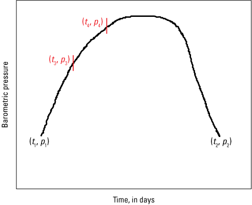
Plot showing a maximum in barometric pressure (p) versus time and two points corresponding to a station occupation at times t3 and t4 used to determine the altimeter barometric correction, Skaergaard intrusion, East Greenland.
Reference Cited
Gettings, M.E., and Parks, H. L., 2025, Aeromagnetic and gravity surveys of the Skaergaard intrusion in East Greenland, 1971: U.S. Geological Survey data release, https://doi.org/10.5066/P91OVG7G.
Appendix 2. Elliptical Cross Section Fitting for Two-Dimensional Models Used to Estimate Glacial Thicknesses and Fjord Depths in the Area of the Skaergaard Intrusion, East Greenland
m
is the slope from equation 2.1, and
d
is depth.
Appendix 3. Gravity Effect of a Two-Dimensional Body of Elliptic Cross-Section Terminated by a Horizontal Line, Skaergaard Intrusion area, East Greenland
U (x, z)
is the gravitational potential at the field point (x, z) for the body with coordinates (ξ,η),
G
is the gravitational constant, and
∆ρ
is the density contrast per unit length.
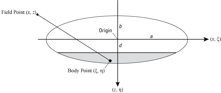
Diagram showing geometry for a two-dimensional gravity model with the cross section having a top truncated by a horizontal line and the bottom a portion of an ellipse. Parameters are the ellipse axes a and b and thickness b–d.
Reference Cited
Abramowitz, M., and Stegun, I.A., eds., 1964, Handbook of mathematical functions with formulas, graphs, and mathematical tables: U.S. Department of Commerce National Bureau of Standards, Applied Mathematics Series 55, 1,046 p. https://hdl.handle.net/2027/uiug.30112061400955 [Reprinted 1965, New York, Dover Publications.]
Appendix 4. Volume of a Wedge of an Elliptic Cylinder Used to Estimate the Relative Volumes of the Various Zones Within the Skaergaard Intrusion, East Greenland
a
is the ellipse semi-major axis and
h
is the height of the cylinder from the base to the intersecting plane.
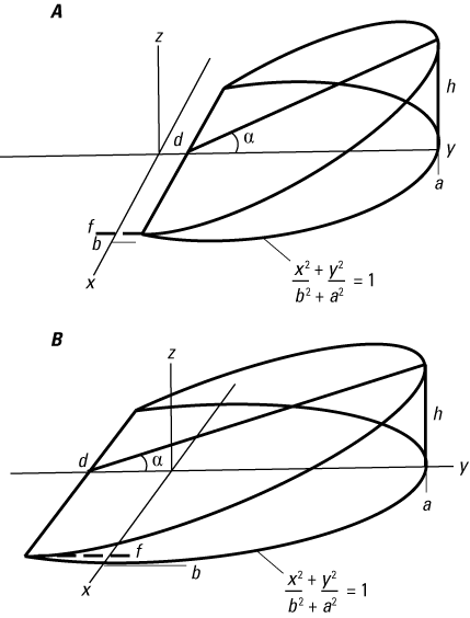
Diagrams showing a wedge of an elliptic cylinder formed by a plane intersecting the cylinder base. A, Diagram of a wedge shorter than the semi-major axis of the ellipse. B, Diagram of a wedge longer than the semi-major axis. The parameters and variables used in the calculation of the volume in appendix 4 are shown.
Conversion Factors
U.S. customary units to International System of Units
International System of Units to U.S. customary units
Temperature in degrees Celsius (°C) may be converted to degrees Fahrenheit (°F) as follows: °F = (1.8 × °C) + 32.
Temperature in degrees Fahrenheit (°F) may be converted to degrees Celsius (°C) as follows: °C = (°F – 32) / 1.8.
Datum
Coordinate information for figures 10 and 11 in this report is referenced to the World Geodetic System 1984 (WGS 84).
For the other figures, vertical coordinate information references sea level high tide marks on the shores. For stations above the sea level mark, vertical coordinate information was obtained by Brunton compass leveling for stations near sea level and by altimetry for those significantly above sea level. Altitude values of peaks on the figures are those from the Danish 1:250,000 scale map sheet (Danmark Geodaetisk Institut, 1969) used to construct the 1:50,000 scale base map. Horizontal coordinate information is referenced to the Danish 1:250,000 scale map sheet.
Altitude, as used in this report, refers to distance above the vertical datum. Altitudes were determined by altimetry except those stations at or near sea level that were determined by Brunton compass leveling.
Observed gravity values are on an arbitrary datum based on the reading of LaCoste gravimeter G-141 on a base station upon return to the United States with no drift control. Drift of both gravimeters was computed using assumed linear drift between closures on the Skaergaard base station or temporary bases such as when working in the Mikis Fjord–Sodalen Valley area, East Greenland.
Supplemental Information
The only topographic map available at the time was the 1:250,000-scale map sheet Gronland 68.0.3 Kangerdlugssuaq of the Danmark Geodaetisk Institut, 1969. This map was made from trimetrogon aerial photography taken by the United States Army Map Service (AMS) in the period immediately after World War II, coupled with ground control from surveys in 1933–34 and place names from 1955 expeditions. The base map used for this report was made from a photographic enlargement of the map sheet to 1:50,000-scale for an area 43 kilometers (km) east-west by 38 km north-south centered on the Skaergaard intrusion, East Greenland.
Moffett Field Publishing Service Center, California, and Baltimore Publishing Service Center, Maryland
Manuscript approved for publication April 14, 2025
Edited by Phil Frederick
Layout by Sarah Lighter
Disclaimers
Any use of trade, firm, or product names is for descriptive purposes only and does not imply endorsement by the U.S. Government.
Although this information product, for the most part, is in the public domain, it also may contain copyrighted materials as noted in the text. Permission to reproduce copyrighted items must be secured from the copyright owner.
Suggested Citation
Gettings, M.E., 2025, Gravity and magnetic surveys of the Skaergaard intrusion, East Greenland: U.S. Geological Survey Open-File Report 2025–1030, 43 p., https://doi.org/10.3133/ofr20251030.
ISSN: 2331-1258 (online)
Study Area
| Publication type | Report |
|---|---|
| Publication Subtype | USGS Numbered Series |
| Title | Gravity and magnetic surveys of the Skaergaard intrusion, East Greenland |
| Series title | Open-File Report |
| Series number | 2025-1030 |
| DOI | 10.3133/ofr20251030 |
| Publication Date | August 20, 2025 |
| Year Published | 2025 |
| Language | English |
| Publisher | U.S. Geological Survey |
| Publisher location | Reston, VA |
| Contributing office(s) | Geology, Minerals, Energy, and Geophysics Science Center |
| Description | Report: ix, 43 p.; Data Release |
| Country | Greenland |
| Other Geospatial | Skaergaard intrusion |
| Online Only (Y/N) | Y |