

Python Hyperspectral Analysis Tool (PyHAT) User Guide
Links
- Document: Report (12.8 MB pdf) , HTML , XML
- Download citation as: RIS | Dublin Core
Acknowledgments
This work was funded through three National Aeronautics and Space Administration’s Planetary Data Archiving, Restoration, and Tools program grants (NNH15AZ89I, NNH16ZDA001N, and NNH18ZDA001N) and received support from the U.S. Geological Survey Community for Data Integration in 2023. We thank Sarah Black, Trent Hare, and others for thoughtful reviews that greatly improved this guide.
Abstract
This report is a user guide for the 0.1.2 release of the Python Hyperspectral Analysis Tool (PyHAT) and its graphical user interface (GUI). The GUI is intended to provide an intuitive front end to allow users to apply sophisticated preprocessing and analysis methods to spectroscopic data. Though the PyHAT package has been developed with a particular focus on laser-induced breakdown spectroscopy (LIBS), the package uses a simple comma separated values (CSV)-based data format and is readily applicable in other spectroscopy applications. This guide provides background information about the package and its capabilities. It also provides practical guidance on usage and example workflows for a wide variety of datasets.
Introduction
Background
The Python Hyperspectral Analysis Tool (PyHAT) is an open-source library developed by the U.S. Geological Survey (USGS) with the goal of providing a single free and easy-to-use source for tools and algorithms that scientists can use to analyze spectroscopic data. Although initially developed for planetary science, PyHAT includes tools that are broadly applicable for planetary and terrestrial remote sensing, as well as laboratory data. PyHAT includes a graphical user interface (GUI) that allows easy access to certain back-end capabilities of the library. The GUI is particularly useful for users who do not wish to develop their own code. The goal of PyHAT is to enable scientists to focus on their core scientific investigation rather than spend time and money on software development or on expensive closed-source software.
PyHAT development has been supported by three National Aeronautics and Space Administration (NASA) Planetary Data Archiving, Restoration, and Tools program grants and received support from the USGS in 2023. The first grant, led by Ryan Anderson, involved the development of analysis capabilities for point spectra and the GUI. A second grant, led by Lisa Gaddis, focused on the analysis of data from orbital imaging spectrometers, such as the Moon Mineralogy Mapper (M3; Pieters and others, 2009) or the Compact Reconnaissance Imaging Spectrometer for Mars (CRISM; Murchie and others, 2007). A third grant, led by Itiya Aneece, expanded on PyHAT capabilities by implementing additional dimensionality reduction, endmember identification, unmixing algorithms, and incorporating these capabilities into the GUI. Funding through the USGS, led by Travis Gabriel, included consolidating orbital and point spectra code; developing documentation, examples, and this user guide; establishing protocols for continuous integration, continuous delivery, and incorporating external contributions; and releasing PyHAT v. 0.1.0. PyHAT was originally designed for the analysis of laser-induced breakdown spectroscopy (LIBS) spectra from the ChemCam and SuperCam instruments on Mars rovers and has received support from those projects. However, updates to the code now ensure that these techniques are broadly applicable to other types of spectra as well, including orbital data used in remote sensing applications.
Motivating an Open-Source Spectral Analysis Tool
Spectroscopic data require specialized analytical techniques, which can be a barrier to their broader use by the scientific community. Scientists may be domain experts, such as having in-depth knowledge of reflectance spectroscopy phenomena, but may not be expert programmers. Furthermore, they may not have funding to pay for expensive software packages and licenses, limiting their ability to interpret spectral data. In the cases where the scientist is also a well-versed programmer, their tools are commonly closed source or are only available upon request, which can compromise reproducibility of their work, set up barriers to access, or create quid pro quo situations.
PyHAT GUI
Alongside the back-end set of modules in PyHAT, which involve a variety of relevant spectral data processing and analysis methods, we have developed the PyHAT GUI, which provides easy access to back-end functionalities for nonprogrammers. Commonly, spectroscopists have a strong visual intuition for their datasets. Therefore, the GUI includes several plotting tools for visual interpretation of spectra and analysis results. The back-end and GUI are installed as a single standalone package.
PyHAT Access
PyHAT is an open-source project hosted and managed by the USGS. The open-source nature ensures these capabilities are readily available to the entire scientific community. In the development of PyHAT, open-access Python libraries are leveraged where possible. When not available in Python, we have translated open-access scripts from other languages. The GUI uses PyQt5 to facilitate user interfacing, and data manipulation relies on the NumPy (van der Walt and others, 2011) and pandas (McKinney, 2010; pandas development team, 2023) libraries. Many of the underlying algorithms used for the analysis of spectra are sourced from the scikit-learn machine learning library (https://scikit-learn.org; Pedregosa and others, 2011) and the PySptools library (Therian, 2018). This guide provides a brief introduction to different methods and algorithms available in PyHAT and the GUI. Readers are referred to the official documentation of scikit-learn, PySptools, and (or) other underlying packages for more detailed information.
Data Format in PyHAT
PyHAT works with data in a simple comma separated value (CSV) tabular format (fig. 1) with each spectrum and its associated metadata stored together in a row. The CSV file has two-level column labels with the top row indicating broad categories of data (by default, “wvl” for wavelength, “meta” for metadata, or “comp” for composition1 ) and the second row indicating more specific categories. For the “wvl” category, the underlying row would contain the wavelength values of the spectrometer and every row thereafter would contain spectral intensities at each wavelength. For “meta” this could include “target name” or other categories. For “comp” this could be “SiO2” or “Quartz” compositional categories for which the user has data. The tool uses the pandas library to efficiently read data in this CSV format into a data frame, making use of the multi-index capability to handle the two levels of column names. Using multi-indexed columns enables the software to easily access large blocks of data—for example, all the spectra in the data frame (all rows and only columns with “wvl”). Another example includes selecting specific metadata columns for each spectrum, such as SiO2 content of all spectra, which is relevant to the analysis of laboratory spectra where the composition is known and included in the metadata. The use of pandas data frames is also helpful for users that access the PyHAT back-end in custom Python scripts, as it provides a familiar and widely used framework for data storage and manipulation.
The default column category names can be changed manually by the user when building a PyHAT spectral object, if needed.
Note that the column names must be unique. The tool does not handle spectra with overlapping spectrometers that have identical spectral channels; that is, for two columns, the first row reads “wvl” and the second row reads an identical numerical value for the spectral wavelength. Users should resolve nonunique wavelengths or other repeated column names outside of the PyHAT tool prior to loading data.
Users may specify the top-level column labels used to indicate spectral data, compositional data, and metadata. By default, spectral data are assigned the top-level label of “wvl,” metadata (if there are any) are assigned the top-level label of “meta,” and compositions (or other metadata types containing continuous numerical values to be used in regression) are assigned the top-level label of “comp.” Composition columns are not required if the user is not regressing the spectral data to compositional data.
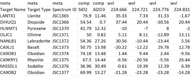
Screenshot of the data format expected by PyHAT and its graphical user interface. Note the two-level column names. This example has been truncated; typically, the spectra (under the “wvl” heading) can have hundreds or thousands of spectral elements (additional columns on the right) rather than only the four listed here. Likewise, metadata (under the “meta” heading) and compositional data (under the “comp” heading) typically can have numerous additional columns. In this example, the “comp” columns contain the oxide weight percentages for the oxides denoted in the second row (SiO2 and Al2O3 in this example). The “wvl” columns contain the spectral intensity values at each wavelength specified in the second row. Negative values are the result of a continuum removal processing step applied to the data.
Interfacing with Hyperspectral Cube Data
PyHAT code is designed to work with data stored in tables as described in the “Data Format in PyHAT” section. However, many planetary (for example, CRISM) and terrestrial (for example, Airborne Visible/Infrared Imaging Spectrometer [AVIRIS]) datasets are collected as hyperspectral cubes, rather than as point spectra. PyHAT includes tools for “flattening” a cube into the native PyHAT spectral object. This converts each pixel in the hyperspectral cube to a row in the PyHAT data table. The row includes the intensity for each spectral band (the spectrum) as well as the x and y pixel coordinates from the original cube. These flattened PyHAT objects can then be used to reconstruct the original cube or to produce output of a single column from the table as a two-dimensional image. Information about the geographic projection of the original data cube can also be stored in the same object with the spectra. PyHAT uses the Geospatial Data Abstraction Library (GDAL) for this functionality, allowing header and metadata information to be retained so that reconstructed cubes or images can inherit the correct projection. This has been tested for cubes from CRISM and M3 datasets. Other datasets may require separate dedicated input/output functionality so that they can be flattened into PyHAT format and retain projection information.
PyHAT SpectralData Object
PyHAT stores data in a Python class named SpectralData. This class is initialized by providing a pandas data frame in the format discussed in the previous section along with keywords to indicate the strings used to label metadata, compositional data, and spectral data as well as a name for the dataset and geographic projection data where relevant. The SpectralData object includes numerous methods that provide a simple way to apply certain functionality to the spectra stored in the object. This simplifies writing custom scripts that utilize PyHAT functionality, and the SpectralData object is also used where possible in the interface between the GUI and the back-end code.
Tool Capabilities
PyHAT’s capabilities are grouped into several categories: data management, preprocessing, classification, regression, and visualization. These categories are also reflected in the top-line menu of the GUI. The categories are briefly introduced here and are discussed in detail in their respective sections.
Data management determines what data will be analyzed and how they will be organized. This includes reading and writing data; looking up metadata; combining, dividing, and organizing datasets; identifying and removing outliers; and identifying endmembers.
Preprocessing includes all steps involved in preparing the spectra for analysis once the data have been ingested into the tool. Whereas data management deals with what data will be used, preprocessing makes changes to the values of the data. For example, spectral masking, baseline removal, calibration transfer, normalization, dimensionality reduction, and unmixing are preprocessing steps.
Classification refers to methods that are used to group similar data within a dataset. It is used in various terrestrial and planetary studies, including mapping land cover, plant species, and minerals. The ability to separate classes depends on spectral variability within and across classes. Classes can be defined by the user, which is necessary when performing supervised classification when the user already knows the features of interest. PyHAT does not currently have supervised classification routines implemented. Unsupervised classification, or clustering, is implemented in PyHAT and is useful when the user does not know which classes to expect in their dataset. With unsupervised classification, spectral samples are divided into a (typically user-defined) number of classes based on some metric that assesses their similarity. Currently the GUI includes the k-means and spectral clustering algorithms.
A major focus of the GUI is to enable users to perform regression analysis of their data. Regression is the prediction of a continuous numerical quantity (for example, the abundance of SiO2 in a target) based on observed spectra. It is a supervised technique that relies on a training dataset for which the spectrum and the quantity in question, SiO2 content in the above example, are both known. This “known” information is used to generate a statistical model that can accurately predict the quantity in question when presented with new spectra. The GUI includes numerous regression algorithms and the ability to run cross validation to ensure that the model parameters are tuned appropriately and that the model is not over-trained so that it performs well on novel data. The tool also allows users to blend the results of multiple submodels to ensure accurate results across a wide variety of targets. We provide an in-depth description of the submodel blending in subsequent sections.
Finally, visualization is essential to allow users to interpret their data using results from the GUI’s statistical analysis. The GUI includes interfaces to plot either rows or columns of the data and to visualize the results of dimensionality reduction, classification, and regression analyses.
Tool Interface
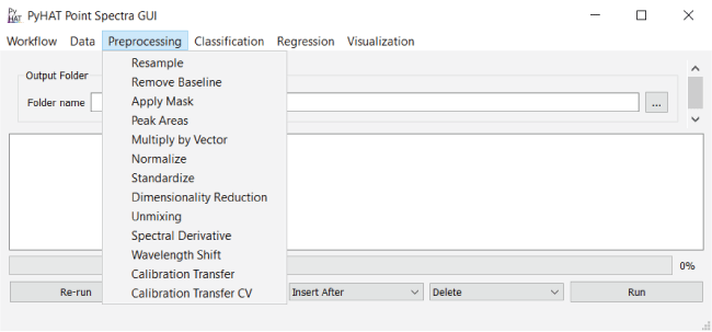
PyHAT can be used without the GUI by importing the back-end library into any Python script. For users who do not wish to write their own scripts, the GUI provides access to many PyHAT capabilities. The GUI is designed around the concept of “workflows”—sets of individual data processing and analysis steps that are applied in a specific sequence to achieve a result (fig. 2). Each step within the workflow is contained in a separate “module,” and these modules can be arranged in any sequence specified by the user, giving the user flexibility to make changes to the logical steps in their analysis. There are logical limitations to this flexibility. For example, principal component analysis (PCA) must be run before PCA results can be visualized, data must be loaded before they can be normalized, and so on.
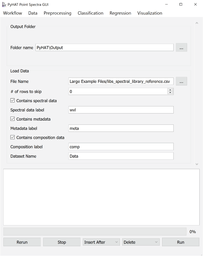
Screenshot showing an example of the PyHAT graphical user interface workflow. The Output Folder module is automatically added to the start of each workflow so the user can choose where output will be stored. Additional modules are added below the Output Folder module in the central part of the interface. In this example, after the output folder is specified, a dataset containing spectral data, metadata, and compositional data is loaded.
The GUI is centered around a main window that contains the workflow modules. Every workflow begins with a module that is automatically added in the main window when the program opens asking the user to set the default path for output. The top-level menu items (or toolbar items for Macs) are workflow, data, preprocessing, classification, regression, and visualization. Selecting an entry from one of these menus adds the corresponding module to the workflow. There are several buttons along the bottom of the GUI: rerun, stop, insert after, delete, and run. These buttons are used to make changes to the workflow and to run the loaded modules. Above these buttons is a progress bar, and above the progress bar is a console window that provides output from running modules and reports any errors. Detailed descriptions of each part of the interface are provided below. Although the exact workflow needed will depend on the data and the task at hand, the end of the guide includes workflow examples that demonstrate how to use the GUI.
Version and Installation
This user guide is for version 0.1.2 of the PyHAT repository, which is available at https://code.usgs.gov/astrogeology/pyhat/-/releases/0.1.2.
Instructions for installation are included in the README.md file in the repository. For updated versions of the code, visit the master branch of the repository at https://code.usgs.gov/astrogeology/pyhat.
Community Support
We encourage users to become part of the PyHAT community through the submission of GitLab Issues. Using this functionality, users can report bugs, suggest improvements, and request assistance. Access to this functionality requires an account on https://code.usgs.gov and a USGS employee must make an account for you. You may contact PyHAT developers to start the process. Install instructions, external developer instructions, and guidelines are included in the repository.
Documentation
PyHAT implements an automated documentation generator that produces HyperText Markup Language (HTML)-based documentation. Documentation is generated based on the markdown files in the repository as well as in Python docstrings, which are large comment blocks at the top of most functions. Docstrings and the HTML documentation provides the user with a description of inputs and outputs, notes, and example use cases. Efforts to improve the HTML documentation are ongoing. Users are encouraged to use GitLab Issues to suggest documentation improvements, or users can assist in documentation directly by becoming a contributor to the repository.
The documentation is hosted at https://astrogeology.code-pages.usgs.gov/pyhat/build-docs/libpyhat.html#module-libpyhat. Alternatively, users can generate a local copy of the documentation using the following commands.
pip install -U sphinx nbsphinx sphinx-rtd-theme
sphinx-apidoc -o docs .
sphinx-build -b html docs public
About This Guide
This user guide is intended to provide an overview of the capabilities of the PyHAT GUI. The GUI serves as a front end for spectral data management, preprocessing, analysis, visualization, and a variety of statistical and machine learning algorithms enabled by the PyHAT library back end. This document describes the conceptual approach of these algorithms and their strengths and weaknesses, but it is beyond the scope of this guide to describe the algorithms in detail. In addition, some of the algorithms rely on abstract mathematical concepts, which are challenging to describe in general terms. Users should (1) refer to the references in this guide for more details on the algorithms and (2) take advantage of PyHAT’s capabilities to experiment with different algorithms and parameters to determine what works best for the task at hand. There is no guarantee that the available algorithms are appropriate for the user’s data, and it is the user’s responsibility to validate and properly interpret the results. This software is under continuous development and the screenshots in this guide may differ slightly from the most up-to-date PyHAT version.
Workflow Menu
The menu options in the GUI are organized from left to right in the approximate order in which they are likely to be used. The leftmost menu is the Workflow menu, which is used to save and load workflows, to open a new GUI window, and to exit the program (fig. 3).
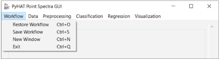
Screenshot showing the PyHAT Workflow menu, allowing the user to restore, save, open a new window, and exit.
Save Workflow
The “Save Workflow” option allows the user to save a workflow for future use. When this option is selected, a dialog window will pop up for the user to navigate to the location in which they want to save the workflow. Workflows are saved as JavaScript Object Notation (JSON) files, so they can be opened in a text editor, if necessary. Doing so is not required in standard PyHAT use.
Restore Workflow
If the user has previously created and saved a workflow of modules within the GUI, it can be restored using the “Restore Workflow” option. When selected, an “Open Workflow File” window pops up with which the user can browse to the workflow file. To avoid conflicts between multiple restored workflows, this option is disabled after one workflow has been restored. The user must close the PyHAT GUI and reopen it to load a second workflow.
New Window
The “New Window” option opens another instance of the GUI window. This can be useful when the user wants to work with multiple workflows or wants to experiment with a module before adding it directly to their main workflow.
Exit
The “Exit” option allows the user to exit the GUI, which can also be done by clicking on the “X” on the window. Workflows are not automatically saved, nor are the datasets or regression models. To save datasets, write to a CSV file using the “Save Data to CSV” option under the Data menu. Workflows and regression models can also be saved as described above and in the “Regression” section, respectively.
Data Menu
The Data menu allows users to load and organize data (fig. 4).
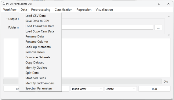
Screenshot showing the PyHAT Data menu, which includes capabilities to determine what data will be analyzed and how they will be organized.
Load CSV Data
The Load CSV Data module allows the user to load a CSV file into the GUI. The user can either enter the path to the file directly into the File Name field or browse by clicking on the button to the right of the field. The user can then enter a name for the dataset. This name will be used to identify the dataset in subsequent modules of the workflow. The dataset name defaults to “Data.”
If the input file contains header rows that need to be skipped, the user can specify the number of rows to skip. Three checkboxes allow the user to indicate whether the file being read contains spectral data, metadata, and compositional data. When checked, a field appears where the user can specify the string used to label these columns in the dataset. If duplicate columns of spectral data (that is, identical wavelength values) are encountered while loading the data, the tool will keep the first (leftmost) column and will notify the user that a column has been removed in the loaded data product.
Save Data to CSV
The Save Data to CSV module allows the user to write output data and (or) results to a CSV file. The user first chooses which dataset to export. The module dynamically reads the top-level column labels from the selected dataset and uses them to populate the list of variables to write. By default, all variables are selected, but the user can change the selection to customize the export. For example, to reduce the file size it may be useful to export just the metadata and predictions for a dataset but not the actual spectra. The user can also specify the name of the file.
Load ChemCam Data
The Load ChemCam Data module allows the user to use the GUI to work with ChemCam (Maurice and others, 2012; Wiens and others, 2012) data, which are available on NASA’s Planetary Data System at https://pds-geosciences.wustl.edu/missions/msl/chemcam.htm. The first field in the module allows the user to specify the search string, and the second field specifies the search directory on the user’s computer. When run, this module will search recursively within the specified directory for files matching the search string and read them into the standard PyHAT format. The default search string “cl5*ccs*.csv” is set to identify CSV-formatted cleaned calibrated spectra (CCS) files with names like those on the Planetary Data System. ChemCam performs most LIBS observations in a series of shots over the same point, such that several points form a raster of points for a given target. The “Averages” and “Single Shots” radio buttons allow the user to choose whether to ingest the average spectra (one spectrum per analysis point) or the single shot spectra (one spectrum per laser shot per point).
After reading the data, the resulting data frame can optionally be written to the output directory as a CSV file. Whether the data are saved to CSV or not, they are also stored in the GUI so that they are available for analysis. The user can specify both the name of the dataset that will be used through the rest of the workflow and the name of the CSV file to which the dataset will be written.
Load SuperCam Data
The Load SuperCam Data module is nearly identical to the Load ChemCam Data module but reads Planetary Data System data from the SuperCam instrument instead. SuperCam data are available at https://pds-geosciences.wustl.edu/missions/mars2020/supercam.htm.
Rename Data
If the user wants to change what a dataset is called within the GUI, the name can be changed using the Rename Data module. Simply choose an existing dataset from the drop-down list and enter the new name into the text field.
Rename Column
Like the Rename Data module, the Rename Column module allows the user to select a new name for an existing column. This is particularly useful to clarify the meaning of a column before subsequent analyses automatically append more columns to the dataset.
Look Up Metadata
The Look Up Metadata module (fig. 5) provides the capability to match metadata from one dataset to metadata in another dataset. For example, this can be useful to match the target name in two different datasets, one that contains spectra for each target and the other that contains their corresponding composition. The spectral and compositional datasets can then be combined to be used in, for example, regression analysis. The user first chooses their datasets in the top-left and bottom-left fields. The user then selects the “Variable to Match” in both datasets; the drop-down list is populated with the existing metadata column names in the corresponding datasets. The columns selected in “Variable to Match” should contain unique strings or numbers that allow the tool to map from the metadata dataset to the primary dataset. It is the user’s responsibility to ensure that the values in the dataset column exist in the specified column of the metadata file. If they are not there, the program will leave those metadata fields blank. Likewise, it is the user’s responsibility to ensure that the identifiers are unique. If they are not, the module will populate each row in the dataset with the first match encountered in the metadata file, which could result in incorrect duplicated metadata and potentially compromise subsequent analyses.
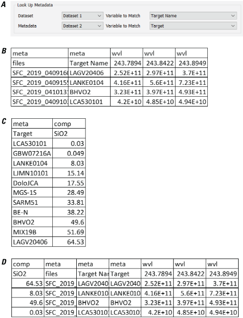
Screenshots showing examples of using the PyHAT Look Up Metadata module. A, The module interface, showing that the “Target Name” column in the dataset named “Dataset 1” will be matched to the “Target” metadata column in the dataset named “Dataset 2.” B, The dataset. C, The metadata. D, The resulting dataset created using the Look Up Metadata module.
Remove Rows
The Remove Rows module allows the user to remove rows from a loaded dataset by evaluating logical operations based on the values of certain variables (fig. 6). The interface for this module begins with a drop-down menu that allows the user to select which dataset to work with. Below the dataset selection menu are one or more rows of drop-down menus that represent individual logical operations. These logical operations dictate which rows to remove from the data. The leftmost drop-down menu in each row is populated with the metadata (“meta”) and composition (“comp”) column names from the dataset selected. Note that for large datasets, this module can be slow to update when a dataset is selected. This is because the module needs to read and parse the selected dataset to populate the leftmost drop-down menu. The next drop-down menu to the right contains a selection of mathematical operators. The third drop-down menu contains the unique values contained in the column selected in the leftmost drop-down menu. Each entry in this third drop-down menu includes unique column values, followed by the number of rows in the dataset that have the identical value. The fourth drop-down menu in each row is used to determine whether an additional filter should be applied to the data. This drop-down menu can be null (containing just a dash symbol) or can contain the word “and.” If “and” is selected, another row of drop-down menus will appear. This allows the user to combine a series of logical filters to remove specific rows in the dataset. When this module is run, the console window will print out the dimensions of the dataset before and after row removal. To examine the modified dataset, the user can then add the Save Data to CSV module to examine the CSV file.
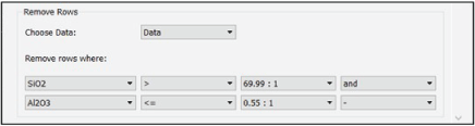
Screenshot showing the PyHAT Remove Rows module. This module allows the user to filter out rows based on logical operations on values of specified variables. In the example, the rows that have a value in the SiO2 column greater than 69.99 and a value in the Al2O3 column less than or equal to 0.55 will be removed. In this dataset, there is one row that has a SiO2 column value of 69.99 and one with an Al2O3 column value of 0.55.
Combine Datasets
With the Combine Datasets module, the user can combine two datasets at a time. The datasets are concatenated via the pandas library using the outer method, such that if one dataset has a column that the other does not have, that column will be retained in the concatenated dataset. For simplicity, the indices (the numerical values assigned to rows of data by pandas when creating data frames) in the original datasets will be ignored and a new index column will be created. If the indices contain information that the user wants to preserve, such as the original order of spectra in the dataset, that information should be stored as a metadata column instead. For more information on this function within pandas, the user can refer to the pandas user guide (pandas development team, 2023).
Identify Outliers
With the Identify Outliers module, the user can identify outliers using the isolation forest algorithm or the local outlier factor algorithm. Outliers may be indicative of poor-quality data, such as in the case of instrument malfunction, anomalous pixels, no signal, and so on. Outliers may also represent valid data that stand out in some way, for example, spectra collected of material standards and compositional extremes. This module only provides the means to identify potential outliers; users should use their expertise to determine whether outliers should be removed from the dataset. The user can use the Split Data or Remove Rows modules within PyHAT or use an external program to remove the rows identified as outliers. The scikit-learn library offers several outlier detection algorithms, including robust covariance, one-class SVM, isolation forest, and local outlier factor. In scikit-learn documentation (https://scikit-learn.org/stable/auto_examples/miscellaneous/plot_anomaly_comparison.html), the local outlier factor and isolation forest algorithms are shown to outperform other outlier identification methods and thus were included in PyHAT.
Isolation Forest
The isolation forest algorithm (Liu and others, 2012) randomly selects features and a threshold value for splitting data into isolated observations (fig. 7). The length of the tree, that is, the number of random splits, needed to isolate the observation is an indicator of whether it is an outlier. Outliers have much shorter trees that are easier to isolate. For more details on this algorithm, refer to the scikit-learn documentation, available at https://scikit-learn.org/stable/modules/generated/sklearn.ensemble.IsolationForest.html. Within PyHAT, the user needs to define the number of estimators and the proportion of the data to treat as outliers. When this algorithm is run, two metadata columns are added to the dataset. One column contains the outlier score, which is a floating-point number that indicates how strongly a given spectrum registers as an outlier. Lower values are more likely to be outliers. The second column is the binary classification of the data into inliers (values of 1) and outliers (values of −1). The fraction of inliers and outliers is specified by the user, and the most appropriate value varies depending on the application.
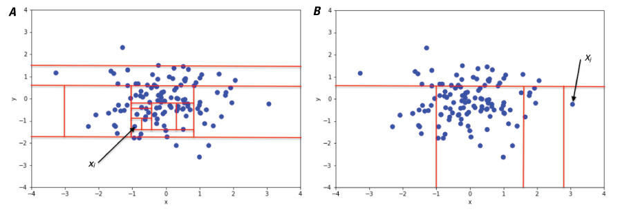
Plots showing a conceptual illustration of the isolation forest algorithm. This illustration shows that isolating a non-anomalous point (xi) in a cluster of points sampled from a two-dimensional Gaussian distribution (A) requires many splits (a longer tree), whereas isolating an anomalous point (xj) (B) requires fewer splits (a shorter tree). Figure from Sal Borelli, reproduced without modification under Creative Commons Attribution-ShareAlike 4.0 International (BY-SA 4.0) license (https://creativecommons.org/licenses/by-sa/4.0/legalcode).
Local Outlier Factor
The local outlier factor algorithm (Breunig and others, 2000) calculates the local outlier factor score for the k number of nearest neighbors around certain observations (fig. 8). The score compares local density with global density of observations. Observations in very low-density areas compared with the global density are potential outliers. Although no single selection for k is best for all situations, 20 works in many cases. In very noisy datasets, a higher value may be more appropriate. This algorithm performs well with high-dimensional datasets. For more information on local outlier factor, refer to the scikit-learn documentation, available at https://scikit-learn.org/stable/modules/generated/sklearn.neighbors.LocalOutlierFactor.html. For this method, the user needs to define the number of neighbors, leaf size, distance metric, and percentage of outliers. Leaf size refers to the number of points at which the algorithm changes its strategy for constructing the tree. Changes to this variable do not affect the results but can have a substantial effect on the execution speed and memory required by the process.
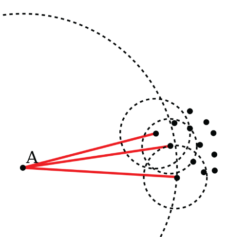
Conceptual illustration of the local outlier factor algorithm. The distance from point A that encloses its three nearest neighbors is considerably larger than the distance from each of those points to their own three nearest neighbors. Thus, point A is likely an outlier. Figure from Wikipedia user Chire, public domain.
Split Data
With the Split Data module, the user can split a dataset by unique values of a certain variable, creating a new dataset for each value. This can be useful for manipulating data as an alternative to removing rows when the user wants to keep both sets of data. For example, the user may want to identify outliers, but retain them as a separate dataset rather than removing them entirely. The Split Data module is also useful when the user wants to isolate individual groups of spectra from the dataset, such as spectra that have been flagged with unique cluster identifications by a clustering algorithm or splitting off an individual spectrum.
Stratified Folds
The Stratified Folds module is used to divide a dataset into N number of groups, also called folds, that can be used to cross validate, train, and test a regression model. This is required to ensure that regression models are generalizable to new data and to determine the accuracy of a model. Refer to the sections below for more detail on cross validation, regression, and the importance of test and train set design. To ensure that the folds have similar distributions of the variable of interest, the data are stratified—that is, they are sorted on a user-specified variable of interest, and then each unique value of that variable is assigned to folds sequentially. Thus, if the data are sorted on SiO2 content, for example, and three folds are desired, the lowest SiO2 value will be assigned to fold 1, the next lowest to fold 2, and so on. Optionally, the user may also specify a secondary tiebreaker variable. This is useful in cases where there are multiple samples with identical values in the primary stratification variable but different properties overall (for example, if there are many different samples with a composition of zero in the primary variable). Specifying a tiebreaker can avoid lumping all of these samples together in one fold. The user can select which fold to use as a test set. This module creates two new datasets, one for the training folds and one for the test fold.
Identify Endmembers
The Identify Endmembers module allows users to identify certain rows as endmembers, which typically correspond to pure spectral signatures. In spectral analysis, users may want to understand how much of a target that has a mixed composition, such as a pixel that includes both rocks and soils, is represented by the individual components, rock and soil in this example, also known as endmembers. In algorithms such as pixel purity index, data are projected in such a way that the most spectrally extreme, and thus spectrally “pure,” pixels are detected and identified as endmembers. Once endmembers are identified, they can be used in unmixing classification methods that estimate the relative contribution of endmembers to a particular spectrum. PyHAT includes several endmember identification algorithms (described below and in table 1): pixel purity index (PPI), N-FINDR, automatic target generation process (ATGP), fast iterative PPI (FIPPI), and sequential maximum angle convex cone (SMACC). To run these algorithms in PyHAT, the user must define the number of endmembers. It is important to note that many endmember identification algorithms at their core are functionally similar yet may nevertheless yield different results; this is because of differences in preprocessing steps, such as the randomization of initial conditions performed in some algorithms (Chang and others, 2016).
An example of the results of each PyHAT endmember identification algorithm is shown in figure 9. This example uses the Salinas Scene dataset (available at https://paperswithcode.com/dataset/salinas, accessed June 26, 2025), which is a high-resolution Earth remote sensing dataset of agricultural lands in the Salinas River valley, California. Although the dataset contains ground truth information, where the endmember compositions are known (that is, each pixel contains a numerical ground truth variable “gt” that refers to a specific type of vegetation) we ignore this information in the example and allow an endmember identification algorithm to find a select number of spectra that represent the endmembers of the dataset. Some algorithms overlap in the identified spectra and others result in unique identifications of endmembers. This figure is purely for illustration purposes because only the raw spectra were used to compute endmembers; preprocessing steps, such as dimensionality reduction, were not performed, likely resulting in poorer performance of certain algorithms. The PPI algorithm, for example, identified two rather similar spectra as endmembers.
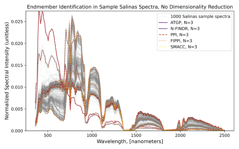
Plot showing results from endmember identification algorithms based on 1,000 spectra from the Salinas Scene dataset, which is included as sample data in the PyHAT repository. Three endmembers were selected for each algorithm (N = 3). No dimensionality reduction or preprocessing steps were performed before endmember identification was performed. Algorithms used are automatic target generation process (ATGP), N-FINDR, pixel purity index (PPI), fast iterative PPI (FIPPI), and sequential maximum angle convex cone (SMACC). Spectra were normalized for visualization purposes.
Table 1.
Description of endmember selection algorithms available in PyHAT.[#, number]
Pixel Purity Index (PPI)
The pixel purity index (PPI) is commonly used for endmember identification because it is semi-automatic and parallelizable (Wu and others, 2014; Chang and Wu, 2015; Chang and others, 2016; Kodikara and others, 2016). Dimensionality reduction, commonly using the minimum noise fraction (MNF) method described below, is usually performed before running PPI to reduce noise and computation costs (Chang and Plaza, 2006). Following dimensionality reduction, the PPI algorithm identifies spectrally pure pixels at the extremes of the data cloud as endmembers (Abe and others, 2014; Molan and others, 2014; Zhang and others, 2015b). This is done automatically several times to obtain a count of how many times a particular pixel is identified as extreme. In terrestrial applications, PPI has been used to identify endmembers for rock types (Singh and Ramakrishnan, 2017), minerals (Molan and others, 2014; Zhang and others 2015b), and vegetation or land cover (Abe and others, 2014; Qu and others, 2014; Marcinkowska-Ochtyra and others, 2017). Similarly, PPI has also been used for determining mineral endmembers on the moon using M3 data (Sivakumar and Neelakantan, 2015; Kodikara and others, 2016).
N-FINDR
The N-FINDR algorithm is commonly used for endmember identification because it is fully abundance-constrained (sums to one and is nonnegative) (Thompson and others, 2010; Ceamanos and others, 2011; Chang and Wu, 2015; Shao and others, 2015; Zhao and others, 2015; Chang and others, 2016). Dimensionality reduction is also recommended before running this algorithm (Zhao and others, 2015). After dimensionality reduction, pixels are iteratively selected to maximize the volume represented inside the data cloud (Remon and others, 2013; Abe and others, 2014). This method has been used for terrestrial (Thompson and others, 2010; Chang and Wu, 2015; Zhao and others, 2015) and planetary (Thompson and others, 2010; Ceamanos and others, 2011) applications for determining mineral endmembers from hyperspectral data, as well as terrestrial applications for land cover types (Shao and others, 2015; Ettabaa and Ben Salem, 2018).
Automatic Target Generation Process (ATGP)
The automatic target generation process (ATGP) is an unsupervised abundance-constrained variant of the PPI and N-FINDR algorithms (Chang and others, 2016) and has several advantages over other endmember identification algorithms. ATGP does not use random initial conditions to initialize the algorithm and simultaneously find all endmembers in a single iteration (Chang and others, 2016). Instead, it finds endmembers sequentially, making it computationally efficient (Chang and others, 2016). Another unique aspect of ATGP for endmember identification is that dimensionality reduction is not performed in the process (Chang and others, 2016). The algorithm determines endmembers by using a pixel similarity metric, where a pixel whose projection is orthogonal to another is dissimilar (Ettabaa and Ben Salem, 2018). ATGP has been used in terrestrial mineral studies (Li and others, 2015; Chang and others, 2016; González and others, 2016) and land cover studies (Li and others, 2015; Ettabaa and Ben Salem, 2018) using hyperspectral data. Additionally, it is used to initialize the fast iterative pixel purity index (FIPPI) algorithm, which is discussed below (Chang and Plaza, 2006; Chang and others, 2017).
Fast Iterative Pixel Purity Index (FIPPI)
The fast iterative pixel purity index (FIPPI), as suggested by the name, decreases the computational time of the traditional PPI. This is done by initializing it with endmembers identified by the ATGP algorithm (discussed above) instead of initializing it with random vectors, which is the traditional approach (Chang and Plaza, 2006; Chang and Wu, 2015; Chang and others, 2017). Additionally, it is an unsupervised algorithm, which does not require the user to manually identify the final endmembers as is required by the traditional PPI (Chang and Plaza, 2006). Lastly, FIPPI is an iterative process, which increases the chances of the final set of endmembers being true endmembers (Chang and Plaza, 2006). FIPPI has been used to determine endmembers for terrestrial mineral (Chang and Plaza, 2006) and vegetation (Chang and Wu, 2015; Chang and others, 2017) studies. Given its advantages over the traditional PPI method, which has been used in many planetary applications, this algorithm may be beneficial to the planetary research community.
Sequential Maximum Angle Convex Cone (SMACC)
The sequential maximum angle convex cone (SMACC) algorithm is an unsupervised linear endmember identification algorithm that is advantageous over other unsupervised algorithms because it requires less a priori knowledge and computation time (Bai and others, 2012) and is more robust to high spectral autocorrelation (Bai and others, 2012). In addition, SMACC does not need extensive parameter tuning to perform well (Thompson and others, 2010). This algorithm determines endmembers by sequentially increasing the volume of a cone in hyperspectral data space to encompass as much of the data space as possible (Lee and others, 2012; Chen and others, 2018). This algorithm has been used to extract endmembers for terrestrial minerals (Thompson and others, 2010; Zazi and others, 2017), rock formations (Chen and others, 2018), and vegetation and land cover (Bai and others, 2012; Bue and others, 2015). In planetary applications, it has been used to study lunar and Martian minerals (Thompson and others, 2010; Gilmore and others, 2011).
Spectral Parameters
Particularly when working with reflectance spectra, it is useful to calculate “spectral parameters” that summarize some aspect of a spectrum into a single value that can then be plotted or mapped to aid in interpretation. Reflectance of a single band, reflectance ratios, slopes, band depths, and band asymmetry are all common spectral parameters. PyHAT implements many predefined spectral parameters that are commonly used with the CRISM instrument on Mars and the M3 instrument on the Moon. CRISM parameters are based on those defined by Viviano and others (2014) and the Interactive Data Language (IDL) code released for the CRISM Analysis Toolkit (CAT; Morgan and others, 2017). Where the two CRISM references differ, we defer to the formulation in the CAT. M3 parameters were provided by Lisa Gaddis (M3 team, written comm., 2023). For convenience, table 2 lists the parameters for M3 and table 3 lists the parameters for CRISM. For details of the parameter calculation, refer to the documentation of the individual spectral parameter functions in the PyHAT code. When calculated, the parameters are added as a new column in the spectral data frame, with a top-level label of “parameter” and a second-level label of the parameter name.
Table 2.
Moon Mineralogy Mapper (M3) spectral parameters.[~, approximately; IR, infrared; µm, micrometer; nm, nanometer; %, percent; UV, ultraviolet]
Table 3.
Compact Reconnaissance Imaging Spectrometer for Mars (CRISM) spectral parameters.[FAL, false color; IRA, infrared albedo; IC2, ices, version 2; IR, infrared; µm, micrometer; TRU, true color; VNIR, visible and near infrared]
Preprocessing Menu
The Preprocessing menu contains a variety of tools used to modify data values prior to using them for analysis (fig. 10). This contrasts with the Data menu, which contains modules used to organize the datasets, but does not actually change the values stored in the spectra themselves. Each preprocessing module is described in detail below.
Screenshot showing the PyHAT Preprocessing menu. Preprocessing steps modify the values of the data and are commonly performed before other analyses.
Resample
In workflows involving multiple different instruments that have different spectral resolutions and overlapping spectral overage, it is useful to resample data from one instrument to the wavelength spacings of another.
The Resample module has a simple interface with two drop-down menus. The first allows the user to choose which data to resample from among the available datasets. The second drop-down menu allows the user to specify which dataset will be used as the reference dataset. When this module runs, it uses the SciPy function scipy.interpolate.interp1d (https://docs.scipy.org/doc/scipy/reference/generated/scipy.interpolate.interp1d.html#scipy.interpinter.interp1d, accessed July 9, 2025) to linearly interpolate the data being resampled onto the wavelengths of the reference dataset. Note that this module will only interpolate between existing data points and will not extrapolate spectra beyond the maximum or minimum wavelength of the original dataset. In situations where the dataset extends beyond the wavelength range of the other, both will be truncated to where they overlap. For example, if the data to be resampled had a wavelength range of 400 to 800 nanometers (nm) and the reference data had a wavelength range of 500 to 900 nm, resampling would result in both datasets having an extent of 500 to 800 nm. When truncation occurs, the program will warn the user by listing the wavelengths of the columns that will be removed in the console window.
Remove Baseline
Spectral data typically consist of three components: baseline, signal, and noise (Shen and others, 2018). Baseline removal, also known as continuum removal, is a common preprocessing step in spectroscopy that seeks to remove signal that contains little to no diagnostic information about the spectral features of interest (Giguere and others, 2015). For example, when working with nongated LIBS data, such as ChemCam data, the spectra contain broad continuum emission owing to bremsstrahlung and ion-electron recombination processes (Giguere and others, 2015). Additionally, baseline removal can be important when working with visible and near-infrared reflectance data, like those from CRISM, especially for comparisons across platforms (Giguere and others, 2015). In the Remove Baseline module, PyHAT includes multiple algorithms that can be used for baseline removal (table 4), which are discussed in detail in the following sections. The code for the algorithms was originally written by C.J. Carey and was provided by T. Boucher (both at the University of Massachusetts at the time). It has been modified to work within PyHAT.
It is challenging to optimize the baseline removal routine because there is no background-free spectrum to compare against. Users should first determine whether continuum removal is appropriate and necessary for their application. As with other algorithms, users should try a variety of approaches and parameters, plot the results, and visually inspect the identified baselines to qualitatively determine which method reliably yields appropriate results. Figure 11 shows an example comparing several different baseline removal algorithms on a LIBS spectrum.
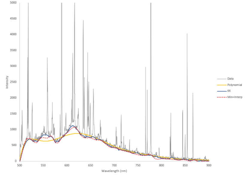
Plot showing the results of several baseline removal algorithms on a laser-induced breakdown spectroscopy (LIBS) spectrum. The raw data are shown in gray. Results from the polynomial, Kajfasz and Kwiatek (KK), and minimum plus interpolate baseline removal algorithms are shown by the colored lines. nm, nanometer. Y-axis is in unitless instrument counts.
Table 4.
Description of baseline removal algorithms available in PyHAT.[FTIR, Fourier transform infrared spectroscopy; LIBS, laser-induced breakdown spectroscopy]
Baseline Removal Algorithms
The following sections describe several baseline removal algorithms available within PyHAT.
Asymmetric Least Squares (ALS)
Asymmetric least squares (ALS) starts by approximating a baseline using Whittaker smoothing (Eilers and Boelens, 2005) and assigning variable weights using a least squares algorithm. It then lowers the weights of the observations that are above the baseline iteratively until convergence occurs. This method works better than other baseline removal methods for Fourier transform infrared spectroscopy (FTIR) data (Giguere and others, 2015) and is fast and reproducible (Eilers and Boelens, 2005). For this method, the user needs to define the asymmetry factor, which determines the relative weight of positive and negative residuals; smoothness, which adjusts the relative importance of the smoothness of the baseline; maximum number of iterations; and convergence threshold parameters. Good starting values for asymmetry are 0.001 to 0.1, and those for smoothness are 102 to 109 (Eilers and Boelens, 2005).
Adaptive Iteratively Reweighted Penalized Least Squares (airPLS)
Adaptive iteratively reweighted penalized least squares (airPLS) (Zhang and others, 2010) works in a similar way to ALS, but adjusts weights of the observations by using the sum of differences between the observations and the baseline. Like ALS, the user selects smoothness, maximum number of iterations, and the convergence threshold for airPLS. Note that the “P” in airPLS is penalized and not partial, as in partial least squares (PLS).
Fully Automatic Baseline Correction (FABC)
Fully automatic baseline correction (FABC) (Cobas and others, 2006) approximates the first derivative of the signal by using a continuous wavelet function. It then does iterative thresholding, which involves finding peak bands with stronger intensities than a user-defined threshold. The baseline is then constructed by running an iteration of weighted Whittaker smoothing, after which mean and standard deviation are recalculated excluding peak bands. For FABC, the user defines smoothness and dilation parameter values. The dilation parameter controls the width of the wavelets used.
Dietrich
The algorithm described by Dietrich and others (1991) is similar to FABC and uses iterative thresholding. The algorithm first applies a moving window smoothing, followed by calculating the squared first derivative. Iterative thresholding is used to find nonpeak points, and binary erosion is applied to the vector of nonpeak points to remove small patches of the spectrum that are incorrectly flagged as baseline. Linear interpolation is then applied to the nonpeak points to form the baseline. This algorithm has outperformed others for preprocessing LIBS data (Giguere and others, 2015). The user-defined parameters for this method are half window, which controls the degree of smoothing applied to the spectrum before calculating the derivative, and number of erosions, which controls the amount of erosion to apply.
Kajfosz and Kwiatek (KK)
The algorithm described by Kajfosz and Kwiatek (1987), originally designed for X-ray near-edge absorption spectra, fits multiple polynomials to approximate a signal and then uses the maximum values to define the baseline. The top width parameter controls the width of the concave-up polynomials used to approximate the baseline, and the bottom width parameter controls the width of the concave-down polynomials used. A value of zero for either top width or bottom width means that type of polynomial (concave-up or concave-down) is not used. The exponent indicates the power of the polynomial and an exponent value of 2 corresponds to parabolas. The tangent indicates whether the polynomials must be tangent to the slope of the spectrum and works best on steeply sloping spectra. It works poorly on spectra with large peaks.
Median
The median algorithm is a simple, model-free way to approximate the baseline, using a user-defined window size to find a local median and smoothing it using Gaussian smoothing (Liland and others, 2010).
Polynomial Fitting
Polynomial fitting is the most common method for baseline correction (Liland and others, 2010). In iterative polynomial fitting, the baseline is found by setting any part of the spectrum that is higher than the polynomial to the value of the polynomial at that wavelength. Once that is done, another polynomial is fit and the process is repeated until a threshold of minimum change is reached. In this module within the GUI, the user specifies the order of the polynomial, the threshold number of standard deviations, and the maximum number of iterations. In general, the overall shape of the baseline is determined by the order of the polynomial, whereas a higher threshold number of standard deviations allows the continuum to be higher than a larger proportion of the spectrum (that is, when the baseline is subtracted, there will be more parts of the spectrum that are negative).
Rubberband
The GUI implements the modified rubberband baseline correction described by Pirzer and Sawatzki (2008). In this method, a convex function is added to the spectrum, the spectrum is divided into segments, the lowest point is determined for each segment, and then these minima are wrapped in a rubber band (convex hull). The bottom side of the hull is used as the approximate baseline. This process is repeated for a user-specified number of iterations. Within the GUI, the user defines the number of ranges and iterations. A larger number of ranges will cause the baseline to fit more closely to small-scale features.
Wavelet à Trous Plus Spline
The wavelet à trous plus spline method approximates the ChemCam baseline removal algorithm described by Wiens and others (2013). It uses the à trous algorithm (Starck and Murtagh, 2006) to decompose the spectrum into a series of wavelet scales (Graps, 1995), then identifies local minima at each of the scales. The nearest local minima in the original spectrum to these wavelet minima are then identified and fit with a cubic spline to determine the baseline to be subtracted from the spectra. The interface for this module allows the user to specify the maximum and minimum wavelet scale to use when searching for minima. It is important to note that the PyHAT algorithm does not perfectly replicate the baseline removal algorithm used by ChemCam, and that the ChemCam data processing pipeline, used to generate the data available on the Planetary Data System, additionally uses different parameters for the baseline removal of the three different spectrometers (Wiens and others, 2013).
Minimum Plus Interpolate
The minimum plus interpolate baseline removal method was developed by the PyHAT team as a simplified alternative inspired by the wavelet à trous plus spline method. The primary difference is that instead of using a wavelet decomposition to guide the identification of local minima in the original spectrum, this method simply divides the spectrum into segments of a specified size, finds the minimum in each segment, and interpolates between them. The user can choose to use a cubic spline, quadratic spline, or linear interpolation function with this module.
Apply Mask
With the Apply Mask module, the user can apply a mask to a dataset to exclude specified parts of the spectrum from analysis. The range of wavelengths to mask are specified in a simple CSV file format (fig. 12). The first column of the file contains the name of the feature to be masked. This column is primarily to make the CSV file more human readable and is not used by the masking algorithm. The second and third columns specify the minimum and maximum wavelengths to mask, respectively. To mask multiple ranges, list them in separate rows of the CSV file. The module reads the CSV file and then steps through each wavelength range, changing the top-level column name for wavelengths from “wvl” (or the user-specified spectral data column label) to “masked.” The data are not removed from the dataset; their labels are simply changed so that the masked data are not used in subsequent calculations. The masking is inclusive (that is, it uses the ≥ and ≤ operators) so if the wavelength range is 200 to 210 nm and a spectral channel has a wavelength of precisely 200 nm, it would be masked. It is generally best practice to choose minimum and maximum wavelength values that fall in between the spectral channels of the data. This ensures that the columns that were masked will not change if a computer rounding error changes the precise value of the wavelength labels for the columns.
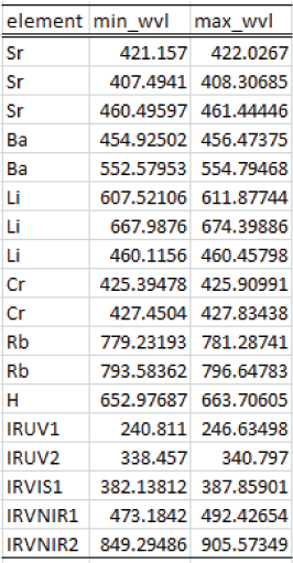
Screenshot showing an example mask file format for the PyHAT Apply Mask module.
Peak Areas
The Peak Areas module implements a version of the method used by Clegg and others (2020) for emission spectroscopy applications to consolidate the data from the adjacent spectral channels on an emission line into a single bin. It is a fast and simple alternative to more precisely fitting individual emission lines in a spectrum and can be useful for collecting data from broad and (or) weak features for use with multivariate methods. It can also make spectra more robust to small wavelength shifts in the peaks (for example, caused by varying instrument temperature) and reduces the size of spectra to enable faster calculations (that is, several spectral bands across a single peak are reduced to a single value).
The method relies on a set of wavelengths corresponding to local minima and maxima, typically derived from an average spectrum (fig. 13A). For each individual spectrum (fig. 13B, colored lines), the data values between each pair of local minima are summed and assigned to the wavelength value of the local maximum within that range (fig. 13B, brackets). Note that because the minima and maxima are based on the average spectrum, they may not correspond to exact minima and maxima for a given individual spectrum (for example, the red spectrum in fig. 13B has peaks that are one pixel away from the peak locations defined by the average spectrum). The average spectrum is used to predefine the bins so that the data are summed into the same wavelength channels for each spectrum.
The default option is for the module to calculate the average spectrum and define the local minima and maxima, but the user can choose to load the values from a file. If the user chooses to calculate the values, they will be written out to a file named peaks_mins.csv. This file can be used to apply the same peak area binning to multiple different datasets. The user can also edit this file to have greater control over the binning ranges.
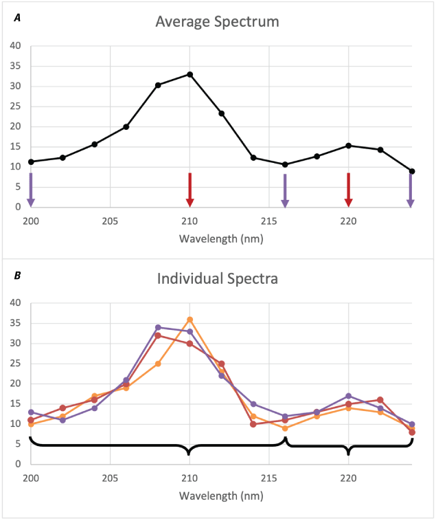
Plots showing an example of peak area binning. A, Example average spectrum. Peaks are marked by red arrows, minima are marked by purple arrows. B, Individual spectra (colored lines and points) are binned (illustrated by the brackets) according to the peaks and minima from the average spectrum, transforming the 13 wavelength channels shown into two channels (not shown) representing the area underneath both peaks. Note that the actual peaks and minima of the individual spectra may differ from those of the average spectrum used for binning. nm, nanometers. Y-axis values are arbitrary intensity for illustration.
Multiply by Vector
The relatively simple Multiply by Vector module allows the user to multiply spectra by a user-provided one-dimensional array of values (vector) from a file. This is useful for applying corrections to the spectra, such as an instrument response function. The vector file has a simple format; the first column contains the wavelengths of spectral channels, and the second column contains the value by which to multiply that spectral channel.
Normalize
The Normalize module divides one or more user-defined spectral ranges by their respective totals, such that for each spectrum, the signal in each range sums to 1. This type of normalization can be used to correct for differing signal levels from different spectrometers and is commonly used in LIBS preprocessing to mitigate fluctuations in plasma emission intensity (Wiens and others, 2013).
Standardize
The Standardize module allows a user to standardize their data such that the spectra in a dataset have a mean of zero and a standard deviation of one (fig. 14). The mean and standard deviation correction factors can be derived from a different dataset if desired (for example, to standardize a test set based on a training set). Standardization is important if the input data have different units and (or) if the user wants all channels to have equal weight. This can reduce the influence of strong spectral features, for example, deep absorption features or strong emission lines, and help to emphasize the variability of weaker spectral features. The user should exercise caution when applying this step because it can also amplify noise—noise can have similar variability as weak spectral features. When this module is run, a new dataset containing the variance and mean vectors is created. To reverse the standardization, the standardized spectra can be multiplied by the square root of the variance vector and added to the mean vector.
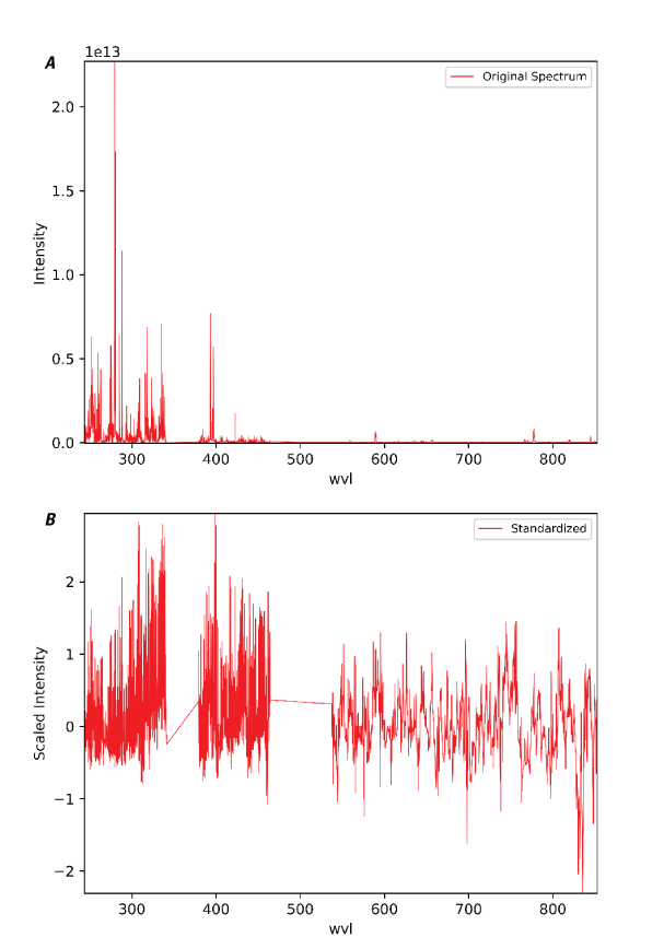
Plots showing an example of the PyHAT Standardize module. A, Original laser-induced breakdown spectroscopy (LIBS) spectrum of basalt prior to standardization. Y-axis is intensity in photons. B, The same spectrum after standardization. Wavelength (wvl) plotted in nanometers.
Dimensionality Reduction
With the Dimensionality Reduction module, data dimensionality can be reduced using various algorithms, which are discussed in the following sections and in table 5. Dimensionality reduction consolidates information from numerous variables, like wavelengths, into a few components. This allows for faster processing and more interpretable results. It can also help with endmember identification and spectral unmixing (Ghamisi and others, 2017). Within dimensionality reduction, there are supervised and unsupervised methods (Shahdoosti and Mirzapour, 2017). In unsupervised methods, such as principal component analysis (PCA) or independent component analysis (ICA), samples do not need to be labeled. Supervised methods, like linear discriminant analysis (LDA), on the other hand, use labeled samples and select dimensions that maximize the distance between classes (Ghamisi and others, 2017).
Dimensionality Reduction Algorithms
Table 5.
Description of dimensionality reduction algorithms available in PyHAT.[#, number; 2D, two dimensional; 3D, three dimensional]
Principal Component Analysis (PCA)
Principal component analysis (PCA) is a linear dimension reduction technique that uses singular value decomposition (SVD). It can be visualized by treating each spectrum as a point in a high-dimensionality space, where each wavelength is a dimension. PCA identifies the axis through the cloud of points in that space along which there is the most variability (fig. 15 illustrates the two-dimensional case). This axis is the first principal component. Subsequent orthogonal axes explain progressively less of the total variation in the dataset. The result is that information from many variables (wavelengths) can be conveyed in a much smaller number of variables (principal components). The values of each spectrum when projected onto the principal components are called the scores, and the vector that is used to project the spectrum and derive the score is called the loading.
The PCA implementation in PyHAT adapts the scikit-learn LAPACK (linear algebra package) method using a full SVD or a randomized truncated SVD depending on the shape of input data and the user-specified number of components. For many datasets in spectroscopy, the first few components explain almost all variability in the data. For more information regarding PCA, refer to the scikit-learn user guide, available at https://scikit-learn.org/stable/modules/generated/sklearn.decomposition.PCA.html.
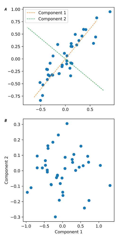
Plots showing an example of principal component analysis (PCA). A, Example of a two-dimensional distribution of data points, showing that components identified by PCA represent the axes of greatest variation of the data. B, Plot of the same data as in A, projected onto the two PCA components.
Independent Component Analysis (ICA)
Independent component analysis (ICA) is a dimensionality reduction method intended to separate d individual sources from mixed signatures. The basic ICA form is X = AS, where X is an n×m matrix such that n is the number of measured signals (spectra) and m is the number of variables (spectral channels), A is an n×d matrix, and S is a d×m matrix of source signals. PyHAT uses two ICA methods. The first is FastICA, as implemented in scikit-learn (Hyvärinen and Oja, 2000). FastICA uses weight vectors to determine one independent component at a time, which is more efficient than other approaches (Wang and others, 2008). Within PyHAT, the user defines the number of components for FastICA. For more information on FastICA, refer to the scikit-learn user guide, available at https://scikit-learn.org/stable/modules/generated/sklearn.decomposition.FastICA.html.
The other ICA method in PyHAT is joint approximate diagonalization of eigenmatrices (JADE; Cardoso and Souloumiac, 1993). PyHAT uses an implementation of JADE translated from Cardoso’s MATLAB version into Python by Gabriel Beckers (https://github.com/gbeckers/jadeR). JADE ICA does not need gradient searches and so is able to converge easily but can be slow for larger datasets (Wang and others, 2008). JADE ICA performs well in extracting the signal from individual chemical elements from LIBS spectra (Forni and others, 2013). As with PCA and FastICA, the number of components is defined by the user.
t-Distributed Stochastic Neighbor Embedding (t-SNE)
Whereas PCA performs linear dimension reduction, t-distributed stochastic neighbor embedding (t-SNE; van der Maaten and Hinton, 2008) is a nonlinear method for representing high-dimensionality data in a two- or three-dimensional map. Whereas the standard SNE uses a Gaussian distribution, t-SNE uses the Student’s t-distribution when it is computationally faster (van der Maaten and Hinton, 2008). The outputs of t-SNE are easier to visualize than other dimension reduction methods because it allows for the visualization of data points that are very close together, and thus similar, as well as those that are very dissimilar. PyHAT uses the scikit-learn implementation of t-SNE, available at https://scikit-learn.org/stable/modules/generated/sklearn.manifold.TSNE.html. The user needs to define several parameters: the number of components, perplexity, learning rate, number of iterations, and number with no progress. The number of components specifies the dimensionality of the embedding and should not exceed three. Perplexity controls the effective number of nearest neighbors used and generally needs to be increased for larger datasets. The learning rate controls the rate of convergence and is typically in the range of 10 to 1,000. Number of iterations sets the maximum number of iterations, and number with no progress allows the algorithm to abort before reaching the maximum number if no progress is being made. Number with no progress is rounded to the nearest multiple of 50.
Locally Linear Embedding (LLE)
Locally linear embedding (Roweis and Saul, 2000) is a commonly used nonlinear dimensionality reduction algorithm owing to its ability to find global optima and its computational efficiency (Qing and others, 2013). PyHAT uses the scikit-learn implementation of LLE, available at https://scikit-learn.org/stable/modules/generated/sklearn.manifold.LocallyLinearEmbedding.html. The user-defined parameters are the number of neighbors, number of components (the dimensionality of the manifold to be used), and regularization. It should be noted that the number of neighbors can have a strong influence on the results and can be challenging to optimize (Qing and others, 2013).
Nonnegative Matrix Factorization (NNMF)
Nonnegative matrix factorization (NNMF) is an additive linear model that is used for dimensionality reduction and unmixing (Gillis and Plemmons, 2013; Wen and others, 2013; Liu and others, 2016a). NNMF does not require a priori knowledge of what is present in the input dataset, and, by enforcing nonnegativity constraints, it has an advantage over other dimensionality reduction techniques in that its results are more physically meaningful (Huang and Zhang, 2008; Liu and others, 2016a). This algorithm can estimate the relative contribution of endmembers to the observed spectra even in scenarios where a spectrum is composed of multiple other spectra (highly mixed), without assumptions of the presence of pure spectra (Ceamanos and others, 2011; Liu and others, 2016a). This is an advantageous attribute for analyzing orbital hyperspectral data when spatial resolution is limited and pure pixels containing a single mineral species are rare. Note, however, that especially in visible and near-infrared spectra, there are complex nonlinear effects and, in general, the results of unmixing such as NNMF should not be interpreted as abundance.
The algorithm deconstructs the input data nonnegative matrix V into two nonnegative matrices H (endmembers) and W (weights, or abundances), whose product approximates V, with W and H remaining nonnegative, and the columns in W summing to unity (Huang and Zhang 2008; Casalino and Gillis, 2017). This algorithm has been used for dimensionality reduction for terrestrial land cover studies (Huang and Zhang, 2008) and for unmixing endmembers for the classification of vegetation and land cover types (Wen and others, 2013, 2016; Zhu and Honeine, 2016), minerals (Liu and others, 2016a), and dusty features on Mars (Ceamanos and others, 2011). Within PyHAT, the user needs to define the number of components and choose whether to add a constant to ensure results are nonnegative.
Linear Discriminant Analysis (LDA)
Linear discriminant analysis (LDA) is a computationally efficient and easily interpretable supervised dimensionality-reduction and classification method (Shahdoosti and Mirzapour, 2017). LDA is also faster than methods like support vector machines (SVM) that require parameter optimization (Zhang and others, 2015a). The algorithm reprojects data into a K−1 dimensional space, where K is the number of classes being separated. It does this in a way that maximizes the ratio of between-class variability to within-class variability, making the resulting dimensions ideal for use in classification.
LDA has been used for a wide variety of applications, including distinguishing subtly different growth stages of insect puparia (Voss and others, 2017) and identifying mung bean varieties (Xie and He, 2018). This algorithm is used in a variety of applications, from land cover studies (Bratsch and others, 2016; Calvino-Cancela and Martin-Herrero, 2016; Shahdoosti and Mirzapour, 2017) to determining chicken embryo gender (Gohler and others, 2017). In addition to these terrestrial applications, LDA has been used for planetary studies, including classification and quantification of analytes in a simulated Martian atmosphere (Benkstein and others, 2014) and mineral classification using CRISM data (Bue, 2014). In PyHAT, the user needs to define the number of components and identify the class column because LDA is a supervised method.
Minimum Noise Fraction (MNF)
Minimum noise fraction (MNF) is commonly used for dimensionality reduction (Das and Seshasai, 2015), especially before endmember identification (discussed above). MNF is also used for noise reduction (Bjorgan and Randeberg, 2015; Hamzeh and others, 2016; Houborg and others, 2016). An MNF transformation consists of two consecutive principal component analyses (PCA), the result of which is a set of MNF components ranked by signal-to-noise ratio (Kale and others, 2017). Removing the noisiest MNF components and reconstructing the image allows for the removal of noise with the retention of information (Parente and others, 2009). This algorithm has been used in a planetary science context to remove noise from Mars lander and rover multispectral observations (Bell and others, 2002; Parente and others, 2009) and orbital hyperspectral data (Douté and others, 2007). To run MNF in PyHAT, the number of components must be defined.
Local Fisher Discriminant Analysis (LFDA)
The local Fisher discriminant analysis (LFDA) algorithm is like the LDA but uses a locality preserving projection (LPP) to preserve data structure while maximizing class separability (Bue, 2014). LPP is a dimensionality reduction technique that finds a linear map that preserves input data structure of neighboring sample points in input data dimensions (Ye and others, 2017) using k-nearest neighbor (Luo and others, 2015). As opposed to other popular dimensionality reduction techniques, such as PCA and LDA, LFDA does not require a unimodal Gaussian data distribution (Luo and others, 2015; Ye and others, 2017). This is particularly advantageous for spectroscopic data analysis because these data are commonly multimodal (Luo and others, 2015). Also, LFDA allows for dimensionality reduction to greater than K−1 dimensions, where K is the number of classes (Bue, 2014). In PyHAT, the user must define the number of dimensions (components), class column, type of metric (plain, orthogonal, or weighted), and number of neighbors.
Unmixing
The Unmixing module within PyHAT provides several algorithms (table 6) that help identify the contribution of endmember spectra to a given spectrum where multiple endmembers may be present; for example, multiple materials within a single pixel of remote sensing data. These algorithms tend to involve two constraints: (1) nonnegativity, which guarantees a zero or positive contribution of each endmember and (2) sum to unity, which guarantees the determined contribution of endmembers sums to one. Unmixing algorithms can also be linear or nonlinear, allowing the abundance of each endmember to affect the composite spectra linearly or nonlinearly (see Schmidt and others, 2014, Goudge and others, 2015, and Liu and others, 2016b, 2018, for examples).
Unmixing Algorithms
The linear unmixing methods implemented in PyHAT—unconstrained least squares (UCLS) and nonnegative constrained least squares (NNLS), where abundances are nonnegative, and fully constrained least squares (FCLS), where abundances are nonnegative and sum to one)—are based on those in PySptools (Therian, 2018). The nonlinear unmixing generalized bilinear model (GBM) is also available in PyHAT and is adapted from Rob Heylen’s MATLAB code (Heylen, 2018). Before running any of these unmixing algorithms in PyHAT, the user needs to run the Identify Endmembers module (described above) or have an a priori list of endmembers. Note that in many cases, particularly for visible and near-infrared spectra, mixing is nonlinear, and the materials present are not fully known; so results from all unmixing methods should be used with caution and should not be interpreted as equivalent to abundance.
Table 6.
Description of unmixing algorithms in PyHAT.[#, number]
Unconstrained Least Squares (UCLS)
The unconstrained least squares (UCLS) algorithm has no rules about the output abundances of endmembers. This means abundances can be negative and do not need to sum to one, which can result in false representations of the abundances of endmembers (Lu and others, 2004). However, this method is good for assessing the quality of endmembers. If results look unreasonable, the endmembers may not be of high quality (NV5 Geospatial Solutions, 2014). UCLS has been used to estimate land cover fractions (Pu and others, 2003) and to assess changes in land cover (Weng and Lu, 2008).
PyHAT uses PySptool’s implementation of the UCLS algorithm for spectral unmixing. This algorithm is useful for the identification or classification of materials in the composite spectra.
Nonnegative Least Squares (NNLS)
In nonnegative constrained least squares (NNLS), abundances are constrained to be nonnegative, which helps results be more interpretable. This algorithm is used to process data from the Thermal Emission Spectrometer (TES) (Ramsey and Christensen, 1998) and mini-TES (Rogers and Aharonson, 2008). It has also been used to estimate green algal bloom area (Pan and others, 2017), estimate material abundances (Benachir and others, 2020), and detect exoplanets (Rameau and others, 2021).
PyHAT uses PySptool’s implementation of the NNLS algorithm for spectral unmixing. This methodology, first outlined by Lawson and Hanson (1974), constrains abundances of the endmembers to be negative for the composite spectra but does not require them to sum to one. Theoretically, this may allow for the identification of missing endmembers or artifacts, such as a dark pixel, which may be included to reach a unity abundance.
Fully Constrained Least Squares (FCLS)
Fully constrained least squares (FCLS), in addition to the nonnegative constraint, requires the sum of abundances to be one. These constraints are commonly referred to as abundance sum-to-one constraint and abundance nonnegative constraint (Khajehrayeni and Ghassemian, 2021). However, in many cases, not all endmembers in a test dataset are represented, and abundances should not sum to one. The FCLS has been used for many applications, including estimating land cover fractions (Kumar and others, 2017; Xu and others, 2018; Khajehrayeni and Ghassemian, 2021), tracking changes in land cover (Zhang and others, 2019), detecting marine oil spills (Cui and others, 2017), estimating mineral abundances (Heylen and others, 2011), identifying hydrous minerals on Mars (Lin and Zhang, 2017), and assessing water ice on Mars (Kereszturi and others, 2011).
PyHAT uses PySptool’s implementation of the FCLS algorithm for spectral unmixing. This methodology produces abundances of the composite spectra that sum to one, making it suitable for estimating abundances in the case of linear mixtures. See Heinz and Chang (2001) for more information on quantification of assumed linear mixtures.
Generalized Bilinear Model (GBM)
Unlike linear mixing models, bilinear models account for interactions between endmembers, assuming that the probability of such interactions are proportional to endmember abundances (Heylen and Scheunders, 2016). The generalized bilinear model (GBM) introduces parameters into the interaction terms that allow the model to be more flexible (Heylen and Scheunders, 2016), while still adhering to the sum-to-one and nonnegativity constraints (Halimi and others, 2011). These parameters help account for abundance, nonlinearity, and noise variance (Halimi and others, 2011). There is also less risk of overfitting with the GBM compared to other bilinear models (Ghamisi and others, 2017). This algorithm has been successfully implemented to unmix land cover and mineral compositions using hyperspectral data (Halimi and others, 2011). Nonlinear mineral interactions are expected in most planetary remote sensing contexts and can be modeled using GBM, though care should be exercised in interpreting unmixing results as true abundances. Within PyHAT, the user must indicate which solver to use: sequential least squares programming (SQLSP) or trust region. The user must also indicate the maximum number of iterations and the number of random starts. More random starts can help to avoid local minima but slows down the calculation.
Spectral Derivative
The Spectral Derivative module calculates a simple approximation of a spectral derivative by finding the difference between each value in the spectrum and the adjacent value, using the pandas diff function. Spectral derivatives are useful for identifying the location of peaks and isolating features from a smoothly varying baseline (fig. 16). When run, this module creates a new dataset containing the derivative spectra. The new dataset has the same name as the original dataset, with the string “ - Derivative” appended.
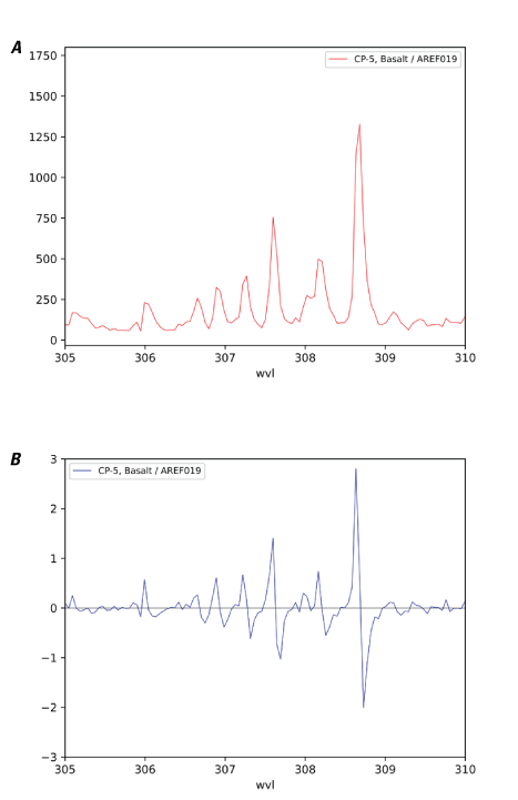
Plots showing an example of spectral derivative. Peaks in the original spectrum (A; y-axis is instrument counts) correspond to locations where the derivative spectrum (B; y-axis is counts per nanometer) crosses zero. Wavelength (wvl) plotted in nanometers.
Wavelength Shift
The Wavelength Shift module allows the user to generate sets of artificially shifted spectra. This can be used to evaluate the robustness of certain analytical steps, such as in cases where the wavelength calibration of data may vary slightly (for example, owing to temperature fluctuations in the instrument). In the text field of the GUI, the user specifies one or more shift amounts separated by commas. When run, this module will add the shift amount to the wavelength values in the column names, then resample the original spectra onto the new wavelengths. This will be done for each of the shifts specified in the user interface, and the resulting data are concatenated and stored in place of the original data. Note that the shifting process results in sections of no data at the end(s) of the spectra, which are automatically cut off.
Calibration Transfer
Scientists commonly need to work with data collected by more than one instrument or under varying experimental conditions (for example, training data collected in a laboratory on Earth being used to interpret data collected by an instrument on a Mars rover). In these cases, simply resampling the wavelengths of the data may not be sufficient—the nature of the spectral response may be different even after instrument response corrections have been applied. However, it can be expensive or impossible to collect training data on both instruments and at all possible conditions. It is therefore desirable to determine a mathematical transformation that can correct spectra collected under one set of conditions so that they can be used with data collected under a different set of conditions. This process is called calibration transfer, and PyHAT provides several different algorithms that can be used for this purpose. The original code for these algorithms was kindly provided by T. Boucher (University of Massachusetts, written commun.). The GUI includes a Calibration Transfer CV (cross validation) module and a Calibration Transfer module.
Calibration transfer relies on a set of spectra of the same targets collected under different conditions. The greater the number of common spectra that are available, the better the results are likely to be. For example, the ChemCam and SuperCam instruments carry calibration targets with them on the rover. Calibration data collected with the flight instrument on Mars can be compared with spectra of identical targets observed under laboratory conditions on Earth and used to derive a calibration transfer model. Calibration transfer can then be used to transform laboratory data to be more Mars-like for calibration with the Mars spectra.
Calibration Transfer CV Module
Typically, the optimal settings for calibration transfer for a given dataset and algorithm are not known a priori. Instead, it is necessary to evaluate a wide range of settings to determine which works best. The Calibration Transfer CV module allows the user to do this by running cross validation on the data. It iteratively removes each spectrum from the data, generates a calibration transfer model using the remaining spectra, and evaluates the performance by calculating the root mean squared error (RMSE). A low RMSE indicates that the transformed spectra are more like the spectra collected under different conditions.
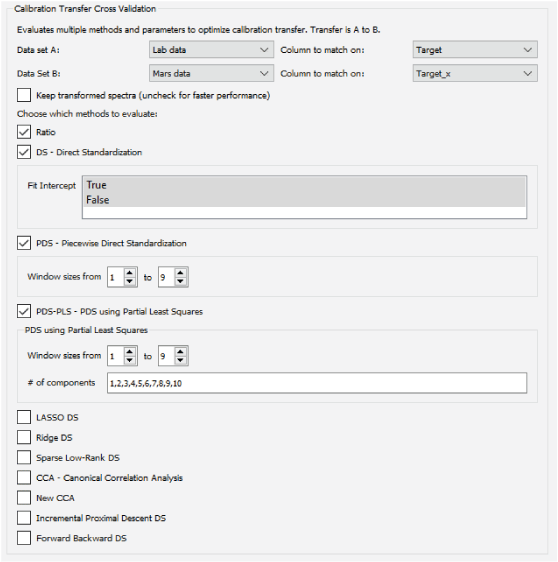
Screenshot of the PyHAT Calibration Transfer Cross Validation module interface with several methods selected.
The interface for this module is shown in figure 17. At the top of the interface, the user can specify the two datasets to use. These datasets should contain spectra of the same targets, observed under two different conditions. Dataset A will be transformed to be as similar as possible to dataset B. The drop-down menus on the top right specify the metadata that will be used to match spectra of a given target in dataset A to the spectra of the same target in dataset B. The module will automatically remove any rows that do not have a corresponding entry in the other dataset. It will also automatically average multiple spectra of the same target together such that the calibration transfer algorithms are working with data frames containing a single average spectrum for each target in both datasets. When the module is running, the console window will inform the user as these preparation steps are being applied.
Beneath the drop-down menus, there is a check box that allows the user to choose whether to keep the transformed spectra as new datasets, or whether just the cross-validation results should be retained. Keeping the spectra can be informative, as they can be plotted to see how a given algorithm and set of parameters transform the spectra, but this option significantly slows down the cross-validation calculation. For better performance when evaluating many algorithms and parameter settings, it is recommended to uncheck this box.
Below the “keep transformed spectra” option there are several check boxes, one for each algorithm to be evaluated in the cross validation (see below for descriptions of these algorithms). Choosing each box will reveal the interface for that algorithm (if there are any parameters). Text fields allow the user to enter multiple comma-separated parameter values and list widgets allow the selection of multiple options so that the user can explore the full parameter space for the selected algorithms. Typically, these fields are populated with the default parameters, but users are encouraged to vary the parameters to suit the calibration transfer task at hand. It is commonly useful to perform a wide-ranging, coarsely gridded search through the parameter space as a first pass, followed by more densely spaced parameters around the settings that give the best initial results.
Calibration Transfer Module
The Calibration Transfer module is similar in layout and functionality to the Calibration Transfer CV module, but it allows only one method to be chosen. In addition, it requires the user to select a third dataset to be transformed by the calibration transfer model based on datasets A and B. The intent is for the first two datasets to contain the samples in common between the two instruments, whereas the third dataset is the data collected on instrument A that is to be transformed to be compatible with instrument B.
Calibration Transfer Algorithms
Several algorithms are available for calibration transfer (table 7). The following sections briefly describe the algorithms. References are provided for users that require additional information. The optimal algorithm for a given situation will depend on the data at hand. The intent of the Calibration Transfer CV module (described above) is to allow the user to compare the performance of the different algorithms and determine which gives the best results.
Table 7.
Description of calibration transfer algorithms available in PyHAT.[#, number]
Canonical Correlation Analysis (CCA)
Canonical correlation analysis (CCA; Hotelling, 1936) is one of the original and most popular methods of transfer learning (Boucher, 2018). CCA projects data into a new space defined by several components in which the correlation between two datasets is maximized. The GUI implements two versions of CCA. The first is the traditional version, as implemented in the scikit-learn library (https://scikit-learn.org/stable/modules/generated/sklearn.cross_decomposition.CCA.html). The second, informally termed “new CCA” is based on a study by Zheng and others (2014) and uses partial least squares as an additional step to identify those components that are most informative. In both cases, the only parameter to set is the number of components to use.
Ratio
The ratio method of calibration transfer is very simple and has no parameters to set. This method simply takes the average of the spectra in each dataset and calculates the ratio to find the average multiplicative factor at each wavelength to transform from A to B. This vector of average factors can then be used to similarly transform any new data collected under conditions like A to be more closely aligned with B. A version of this method is used to apply the “Earth to Mars” correction to ChemCam laboratory data so that it can be used for regression with data collected on Mars (Clegg and others, 2017).
Direct Standardization (DS)
Direct standardization (DS) is a simple and commonly used method of calibration transfer. It uses a single transformation matrix F to transform data from instrument A to instrument B (Wang and others, 1991), such that:
In the GUI, the only parameter that needs to be set by the user for DS is whether to fit the intercept (that is, include a constant in the transfer function) or not.
Piecewise Direct Standardization (PDS)
Although the DS method is popular, its multivariate objective function is generally underdetermined (that is, there are more spectral channels than there are spectra in common between the two different conditions), which makes it difficult to obtain a good transformation of the spectra (Wang and others, 1991). In addition, it uses information from the entire spectrum to determine the transformation applied to a given wavelength, which is physically not realistic—each spectral value on one instrument is likely to be meaningfully related to only a small surrounding region of the spectrum from the other instrument. Piecewise direct standardization (PDS) mitigates these problems by using a sliding window. The transform applied to each spectral channel is a least squares regression problem, using the several spectral channels around the channel of interest to determine the transformed value. The full calibration transfer is the result of the numerous small regression problems. In effect, the transfer matrix derived by PDS as compared to DS has most cross correlations (off-diagonal elements in the covariance matrix) set to zero (Wang and others, 1991).
The PDS interface in the GUI requires the user to specify the size of the sliding window to be used. In the cross-validation interface, the user specifies a range of values. Every odd number in the specified range will be tested as a window size.
PDS with Partial Least Squares (PDS-PLS)
PDS can result in transferred spectra with sharp changes that are not physically realistic. These can arise from the fact that the solution is a combination of several regressions along windows; this effect can be minimized by using a regularized regression method to solve the least squares problems (Boucher and others, 2017), such as partial least squares (PLS) (Wang and others, 1991; Boucher and others, 2017). In addition to the sliding window size, when using PDS-PLS, the user must also specify the number of components (latent variables) to use in the PLS models. The cross-validation interface thus expects additional data, in the form of a comma separated list of component numbers (integers), which allows models with different numbers of components to be evaluated.
Least Absolute Shrinkage and Selection Operator (LASSO) DS
One way to improve upon DS is by adding a penalty when calculating the transfer matrix, which can encourage desirable behaviors, such as sparsity or smoothness in the results (Boucher and others, 2017). Sparsity in this context refers to solutions where many of the values are zero. Sparse solutions require less computation time and increase interpretability. Sparse results are encouraged by including a penalty based on the L1 norm (the sum of the absolute values of the regression coefficients). Regression using this penalty is referred to as least absolute shrinkage and selection operator (LASSO) regression. Refer to the description of LASSO in the “Regression Algorithms” section below for more information on this method. The LASSO DS, ridge DS, and sparse low rank DS algorithms are all related and, as implemented in PyHAT, are solved using the same underlying function, and therefore have the same parameters. The parameter ρ controls the rate of convergence, the ratio of β over ρ controls the strength of the penalty, and ε sets the threshold for convergence. The user can also set the maximum number of iterations, which determines how long the algorithm will keep trying to converge. In practice, the user should experiment with these parameters to determine which yield the optimal transformation.
Ridge DS
Ridge regression uses the L2 norm (the Euclidean distance) rather than the L1 norm used by LASSO (see description in the “Regression Algorithms” section below for more detail). Whereas the L1 or LASSO penalty has the effect of encouraging sparseness, the L2 or ridge penalty encourages smoother regression coefficients with decreased variance, which tend to be more physically realistic (that is, the transform applied to one spectral channel should be similar to that applied to its neighboring channel) (Boucher and others, 2017).
Sparse Low Rank DS
The spectra from different instruments or conditions can be approximated by projecting them into a lower dimensional space, like principal component analysis (PCA; see the section on dimensionality reduction). This lower dimensionality approximation of the spectra is referred to as a low-rank approximation and can promote efficiency and interpretability of calibration transfer (Boucher, 2018). Although low-rank matrices are not commonly sparse, sparse matrices and low-rank matrices are both used to encourage simpler, easier to interpret results (Richard and others, 2012). Low-rank DS can be sensitive to noise, but the addition of a sparse regularizer makes the low-rank DS method more robust to noise (Boucher, 2018). A combined method, sparse low rank DS uses the “trace-norm” (the sum of the singular values of the regression matrix) penalty described by Richard and others (2012) to take advantage of both methods.
Forward-Backward DS
Forward-backward proximal descent DS and incremental proximal descent DS are related to sparse low rank DS. They similarly combine an L1 norm penalty with the trace-norm penalty but use different approaches to solving the optimization problem (Richard and others, 2012). The parameter t is the step size, svt controls the threshold for the singular value thresholding (Cai and others, 2010), L1 controls the threshold value for soft thresholding (Boucher and others, 2017), ε is the convergence criterion, and number of iterations determines how many iterations to try.
Incremental Proximal Descent DS
The forward-backward DS method can be inefficient because it has a large memory footprint (Richard and others, 2012). In such cases, the incremental proximal descent DS can be used with similar results (Bertsekas, 2011; Richard and others, 2012). This method uses the same input parameters as forward-backward DS.
Classification Menu
Classification involves grouping similar data, either into predefined categories by comparison with training data that have already been labeled (supervised classification) or into categories dictated by the structure of the data (unsupervised classification, also known as clustering). Currently, two unsupervised clustering algorithms are available in the GUI. No supervised classification algorithms are listed under the Classification menu, but an inactive entry serves as a placeholder for the potential addition of supervised classifiers.
K-Means
K-means clustering is one of the most used clustering methods. It seeks to divide the data into a user-specified number of clusters (k) of equal variance. It works by starting with k cluster centroids, randomly distributed in the same space as the spectra to be classified (fig. 18). Each point is assigned to the nearest cluster centroid, and then a new centroid is calculated for each cluster, based on the spectra assigned to that cluster. This process is repeated until the centroid no longer changes with each iteration, within the user-specified tolerance value. It is recommended (though not required) that dimensionality reduction be applied to the spectra and k-means be run on the reduced dimensionality values rather than the full spectra. This significantly speeds up the calculation and can be used to ensure that clustering is based on meaningful values rather than noise (for example, by using the first several PCA components, which explain most of the variance in the data). K-means is susceptible to finding local minima, so typically the algorithm is run numerous times and the result with the minimum sum of squared distances in each cluster is used. K-means assumes that the clusters in the data are convex and isotropic, so it can give poor results when the actual cluster in the data are elongated or have irregular shapes.
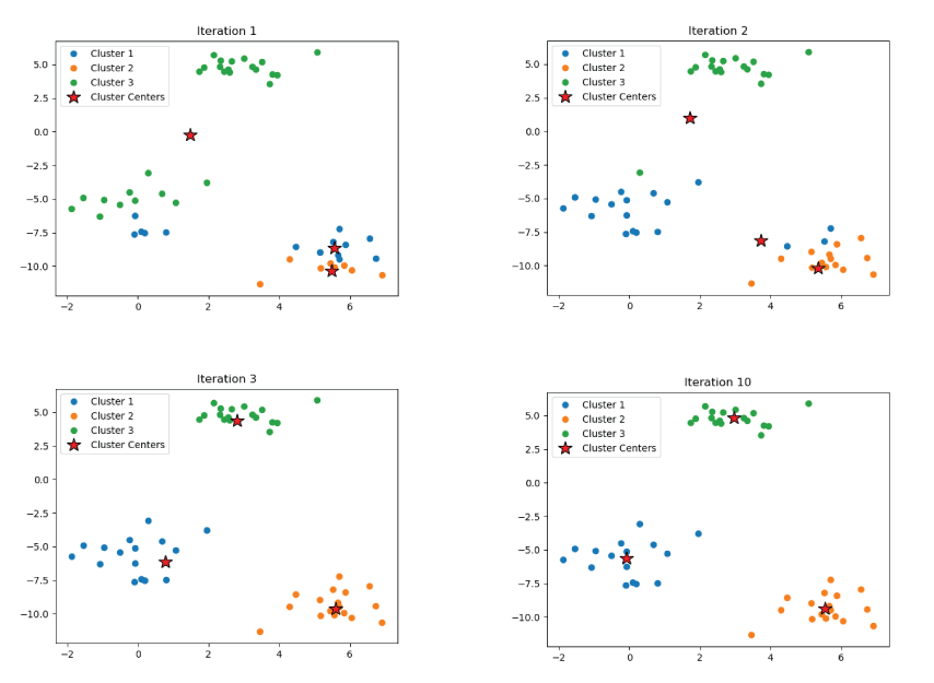
Plots showing an example of the k-means clustering algorithm. Initially the cluster centers are randomly distributed and do not correspond well to the data. Subsequent iterations update the cluster centers until they correspond well to the centers of the actual data clusters.
Spectral
Spectral clustering is an alternative to k-means clustering that performs well when clusters have complex shapes that are poorly described by the cluster center and spread. PyHAT uses the scikit-learn implementation of spectral clustering, available at https://scikit-learn.org/stable/modules/generated/sklearn.cluster.SpectralClustering.html. Like k-means, the user can specify the number of clusters and the number of runs of the algorithm to use. Spectral clustering works by generating an affinity matrix between the data points and embedding it in a low-dimensional space where simple clustering like k-means is more effective. The user can select from several kernels to be used to generate the affinity matrix: radial basis function, nearest neighbors, sigmoid, polynomial, linear, and cosine. These kernels are described in the scikit-learn documentation, available at https://scikit-learn.org/stable/modules/metrics.html. In general, most kernels define a symmetric function that determines the similarity between points in such a way that closer points are given greater weight than more distant points. The parameters associated with the kernels adjust this falloff in sensitivity. In practice, the user can experiment with the parameters to get acceptable results.
Regression Menu
Multivariate regression is concerned with predicting the value of a dependent variable (y) based on the value of multiple independent variables (x). In the context of spectroscopy and chemometrics, the independent variables are typically the spectral intensity in each wavelength bin (though other data may also be used), and the dependent variable is some physical property of the material being observed. For example, for ChemCam and SuperCam data, multivariate regression is used to create a statistical model relating LIBS spectra to their chemical compositions. The development of regression models is one of the primary purposes of the GUI.
A regression model is typically generated based on a training set—a set of spectra for which the value of the dependent variable of interest has already been independently measured. These spectra can then be used as the input to regression algorithms that identify relations between the individual spectral channels and the dependent variable. PyHAT has many tools available for running regression analyses (fig. 19), which are detailed below.
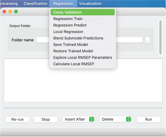
Screenshot showing the Regression menu options for regressions currently available in PyHAT. This example also illustrates that the menu options on Mac machines are located in the desktop menu bar and not on the applet itself.
Overfitting and Accuracy
Overfitting occurs when model complexity is increased (or other model parameters are tuned) such that the model performs well on the training set but fails to predict new data accurately. This is analogous to using a high-order polynomial to fit noisy data (fig. 20); the polynomial may fit the training data perfectly (black points in fig. 20), but it does not accurately capture the underlying trend and may give inaccurate results for new x values (red point in fig. 20).
Similarly, calculating the root mean squared error (RMSE) of the model’s predictions of the training data (also known as RMSE of calibration [RMSEC]) can give an incorrectly optimistic estimate of the model’s accuracy. In the case of the overfitted polynomial, the RMSEC would be zero, suggesting that the model is perfect, when the performance on novel data shows that it is not.
To avoid overfitting, cross validation (described below) should be used to tune the model parameters, and an independent test set should be used to assess model accuracy. The RMSE of the test set is also known as the RMSE of prediction (RMSEP). The test set is data that the model has never seen before—it should not be used to tune the model parameters, only to assess the performance of the tuned model.
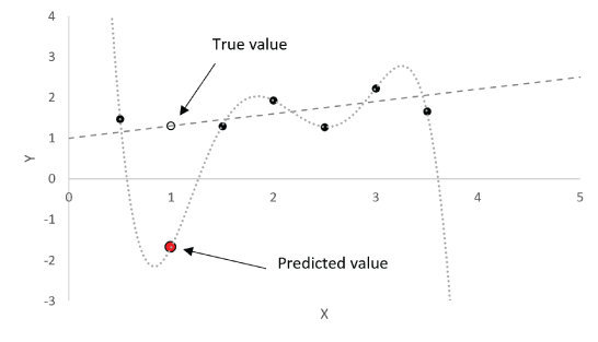
Plot showing an example of overfitting with a polynomial regression (curved dashed line). The straight dashed line indicates the true linear trend of the data. The polynomial function fits the training data (black points) perfectly but would lead to an erroneous prediction at X = 1 (red point), whereas the correct prediction for X = 1 would fall on the dashed line (open black circle). Multivariate regression models can suffer from the same behavior, and thus parameters must be tuned with care, and model accuracy should be assessed with an independent test set.
Cross Validation
Cross validation is an essential step in optimizing a multivariate regression model and ensuring that the model is not overfitted to the training data. In cross validation, a subset of the training data is held out and treated as unknown. A model is then trained on the remaining data and used to predict the held-out data. This process is repeated iteratively so that every piece of training data is held out as an unknown once. The result is an estimate of how a model trained on the full training set will perform on novel data—the root mean squared error of cross validation (RMSECV). By repeating this process for different parameter settings for a model, the optimal settings (those that minimize RMSECV) can be determined. RMSECVs can also be compared between models to determine which gives the best results for the task at hand.
PyHAT implements stratified k-fold cross validation. The Stratified Folds module, described above, is used to split the data into training and test folds with similar distributions of the dependent variable of interest. One fold is completely held out as a test set to evaluate the performance of the final optimized model (RMSEP). The remaining folds are used for cross validation to tune model parameters and compare different regression models.
In the interface for regression cross validation, the user can specify which of the regression algorithms to use. For each algorithm, several parameters can be specified. By entering comma separated values in text fields or selecting multiple entries in list boxes, the user can determine all the permutations to be evaluated. Note that for some models and parameter settings, cross validation can be time consuming. The console window will display updates on the progress of the cross validation.
Regression Train
If the user already knows the optimal parameters for training a regression model, they can bypass cross validation and train a single regression model. The same algorithms are available as for cross validation; the primary difference is that only one algorithm can be chosen at a time, and each parameter accepts only a single value rather than a list of values. As with cross validation, the range of values for the dependent variable can be adjusted to permit a specialized regression model to be trained on a restricted range of input data. Note that the Regression Train module trains a regression model but does not perform predictions.
Regression Predict
Once the regression model has been trained by either using cross validation or regression training, the user can apply the model using the Regression Predict module. This module allows the user to choose from a list of trained regression models and use the selected model to predict the results for one or more datasets. The predicted results are added to the selected datasets as a column, with a top-level label of “predict” and a second-level label specifying the regression model used.
Local Regression
Local regression is somewhat different than the other regression methods available in PyHAT that are described below. Rather than deriving a single regression model to predict all new data, local regression derives a new model to predict each individual spectrum, trained on spectra from the training set that are most like the unknown spectrum being predicted. This similarity is quantified as the Euclidean distance between the spectra in the high-dimensional space defined by the spectral channels. This algorithm was developed by the PyHAT team and draws inspiration from the LOCAL algorithm (Shenk and others, 1997), in which a weighted average of PLS models is used.
PyHAT implements local regression using the elastic net algorithm. Elastic net was chosen because, in addition to its advantages described below, scikit-learn includes an implementation of elastic net that runs its own internal cross validation to set the α parameter. By leveraging this capability, the local elastic net algorithm can train many elastic net models, each of which optimizes its own α parameter with no need for human intervention. The key user-specified parameter for local regression is the number of nearest neighbors. This specifies the nearest N spectra from the training set to use to generate the model that will be used to make predictions on each unknown spectrum.
Since it calculates many individual models, local regression can be time consuming, particularly when cross validating to choose the optimal number of nearest neighbors. It is commonly useful to apply peak area preprocessing prior to running local regression to reduce the size of the spectra and increase the calculation speed.
Blend Submodel Predictions
The Blend Submodel Predictions module allows the user to implement the submodel regression approach described by Anderson and others (2017). This approach is useful when the unknown data to be predicted may exhibit a wide range of values for the dependent variable, such that a single regression model would have trouble accurately handling all possible cases. Instead, by training multiple regression models, each on a restricted but overlapping range of values, the results can be blended to yield a more accurate prediction across all values. This method uses a reference model trained on the full range of dependent variable values (for example, 0–100 weight percent for a regression model predicting the SiO2 content in a target analyzed using LIBS) as an initial guess of the true value. This initial guess is then used to determine which more specialized model (submodel) should be used to get a more accurate result. If the reference model predicts a value that falls in between a specified overlap range between two submodels, the submodel predictions are blended using a linear weighted average. This overlap range is a free parameter that can be optimized; it does not necessarily have to correspond to the overlap in training data ranges for the submodels.
This module does not perform predictions; it combines predictions that have already been run using the Regression Predict module. When the user selects a dataset, the prediction columns are read from that dataset and used to populate the drop-down lists of predictions for the reference model and submodels. The interface begins with just a reference model and a low and high submodel. If the user wants to use predictions from additional submodels, they can click the “Add submodel prediction” button, which will insert a new row between the low and high submodels. For each submodel, the user must specify the range over which it should be used. Thus, for a low model trained on 0–50 weight percent SiO2, you might choose 50 as the maximum value for that model. For a middle submodel trained on 40–60 weight percent SiO2, those ranges should be entered as the minimum and maximum values. The ranges selected for the submodels must overlap for this method to work. If they do not overlap, it is possible for the reference model to predict values that do not correspond to any submodel.
In practice, most users will want to optimize their blending ranges to get the best possible results. This can be done by predicting the training data and then selecting it in the Blend Submodel Predictions module. Load the desired submodel predictions and then select the “Optimize” check box. This will bring up an additional drop-down list, where the dependent variable of interest can be selected. When the module runs, it will start with the minimum and maximum blending ranges provided in the user interface for each submodel and adjust them to minimize the error in predicting the variable of interest. The progress of the optimization is printed to the console window. Once the optimal ranges have been determined using the training data, they can be used for other datasets. Note that optimization should not be applied on test set data; doing this will tune the blended results to give the best possible test set results, and thus the model settings will no longer be independent of the test set.
Save or Restore Trained Model
If desired, trained regression models can be saved to a user-specified binary file. This file can be restored using the Restore Trained Model module. When a file is selected in this module, information about the model in that file is displayed in the console window.
Regression Algorithms
The following sections provide a brief overview of the available regression algorithms in PyHAT. PyHAT relies heavily on the scikit-learn library for these algorithms. It is beyond the scope of this guide to describe the details of each algorithm. Instead, the focus is on practical considerations when using the algorithms as implemented in PyHAT. Additional information and documentation on these methods can be found in the scikit-learn documentation, available at https://scikit-learn.org/stable/index.html.
In most cases, trained linear regression models result in a vector of regression coefficients (w) that, when multiplied by a spectrum (x), yield a predicted y value:
It can be informative to plot the regression coefficients as a function of wavelength to see which parts of the spectrum have the strongest influence on the predicted results. Thus, when a regression model is trained in PyHAT, the regression coefficients are added to a new dataset labeled “Model Coefficients.” Rows from this dataset can be plotted using the Plot Spectra module, or the data can be saved to a CSV file and analyzed using another program.
Table 8 provides a high-level summary of the available regression algorithms and their properties.
Table 8.
Description of regression algorithms available in PyHAT.[#, number]
Ordinary Least Squares (OLS)
This is the simplest form of multivariate regression. It seeks to find the regression coefficients w:
that minimize the sum of squared residuals: where, for each observation i of the full set of m observations, spectra are represented by x with n spectral channels and the value being predicted (for example, composition) is y. E in equation 4 represents the error in the prediction. The only parameter for this regression method is a discrete choice regarding whether to fit the intercept; that is, whether w0 should be fixed at zero or free to vary. Ordinary least squares (OLS) tends to perform poorly when there is a high degree of correlation between the features in the data, which is common among spectroscopic data.Partial Least Squares (PLS)
Partial least squares (PLS) is a linear regression method closely related to PCA that works well in situations where there is a high degree of correlation between the independent variables (x) and where there are more independent variables than there are observations. Both situations are common in spectroscopy.
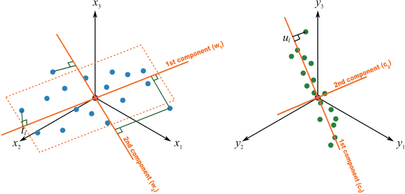
Plots showing an example of partial least squares (PLS) regression. PLS is similar to principal component analysis except that the components are chosen so that they best explain the data in both x and y directions. Figure from Process Improvement Using Data website by (and copyright of) Kevin Dunn (https://learnche.org/pid/latent-variable-modelling/projection-to-latent-structures/conceptual-mathematical-and-geometric-interpretation-of-pls), reproduced without modification under Creative Commons Attribution-ShareAlike 4.0 International (BY-SA 4.0) license (https://creativecommons.org/licenses/by-sa/4.0/legalcode).
Like PCA, PLS projects high-dimensionality data into a lower dimensionality space (fig. 21). The difference is that in PLS both the x and y variables are projected into a new space, and the axes through the cloud of x data points are chosen such that they correspond to the greatest variation in the y space.
There are several different algorithms for PLS; PyHAT uses the nonlinear iterative partial least squares (NIPALS) algorithm (Wold, 1975) as implemented in the scikit-learn PLSRegression function.
The key parameter for any PLS model is the number of components or latent variables. A model with too few components will not adequately capture the complexity of the data and will not result in accurate predictions. A model with too many components will be overfitted, performing well on the training set (low RMSEC) but failing to predict new data accurately (high RMSEP). Thus, it is important to use cross validation to tune the number of PLS components appropriately.
Least Absolute Shrinkage and Selection Operator (LASSO)
Least absolute shrinkage and selection operator (LASSO) is a linear method that solves the OLS minimization as above but with the addition of a regularization term consisting of a constant (α) multiplied by the L1 norm (the sum of the absolute value of each element) of the coefficient vector:
The result is a sparse model, for which only a small number of coefficients are nonzero. Essentially, LASSO performs feature selection as an inherent part of the process of training the model. The resulting regression model is typically easier to interpret, but which can still achieve accuracies comparable to or better than other methods.
The scikit-learn implementation of LASSO in PyHAT uses coordinate descent to fit the model. The PyHAT cross validation interface for LASSO asks the user to specify a range of α values and the number of α values to distribute logarithmically in that range. Variable α controls how strongly the L1 norm term is weighted, effectively controlling how sparse the solution is (eq. 6). Cross validation results can then be assessed by plotting the RMSECV as a function of α for each permutation of other parameters to find the optimal setting. LASSO also has the option of fitting the intercept and of forcing all coefficients to be positive. Forcing the coefficients to be positive and not fitting the intercept can be useful when a model must give only positive results; however, this may sacrifice some accuracy.
Ridge Regression
Like LASSO, ridge regression applies an additional regularization term to the least squares minimization function (eq. 5). In the case of ridge regression, the additional term is a constant multiplied by the L2 norm (Euclidean norm or sum of squared values) of the regression vector:
The effect of this additional term is to shrink some of the regression coefficients, making the model more robust to multicollinearity (many predictor variables being correlated with each other) in the data than OLS. However, unlike LASSO, ridge regression is not able to set coefficients to zero, so it does not result in a sparse set of coefficients. Ridge regression does not benefit from the same efficiencies in computing regression coefficients as LASSO and elastic net (described below), and thus cross validation can be more time consuming. For efficiency, it is commonly useful to first evaluate the cross-validation performance with a relatively small number of α values, and if necessary, repeat the cross validation with a more restricted range of α values once the approximate behavior is known.
As with many regression methods, the user has the option of choosing to fit the intercept. Ridge regression also includes a normalization option. If this option is selected, the spectra will be mean-centered and divided by the L2 norm.
Elastic Net
Elastic net is a hybrid of LASSO and ridge regression. It uses both the L1 regularization term from LASSO regression and the L2 regularization term from ridge regression, where the weight applied to each is determined by the L1 ratio parameter (ρ):
Elastic net with ρ = 0 would be equivalent to ridge regression, whereas ρ = 1 would be equivalent to LASSO regression. By using both L1 and L2 regularization, elastic net can derive a relatively sparse model while also keeping the stability that comes from ridge regression’s L2 regularization. One benefit of elastic net over LASSO applies when there are multiple highly correlated variables—LASSO will tend to randomly choose one of these variables and ignore the rest, whereas elastic net will choose all of them.
The interface for elastic net is like that for LASSO, with the addition of the L1 ratio. Cross validation of elastic net can be time consuming owing to the additional permutations introduced by the L1 ratio parameter.
Bayesian Ridge Regression (BRR)
Bayesian methods calculate distributions rather than fixed values for both model parameters and predicted values. This has the benefit of providing uncertainties for each predicted value. As the name suggests, Bayesian ridge regression (BRR) is a generalization of ridge regression (it imposes the L2 norm constraint; Zou and Hastie, 2005; Efendi and Effrihan, 2017). The key parameters for BRR are α and λ, which correspond to the precision of the distributions for noise in the data and the weights of the model, respectively. These are both assumed to have a gamma distribution, controlled by shape parameters (α1 and λ1) and inverse scale parameters (α2 and λ2). However, the user typically does not need to set these parameters. They are set as uninformative priors that will be optimized when the model is fit. In the PyHAT GUI, the α and λ parameters are hidden by default, but can be set by the user if desired by unchecking the “Use default” boxes. The user may also adjust the number of iterations and tolerance, though this likewise is not typically necessary. Users can also select whether to fit the intercept and (or) normalize data, like in other regression methods.
Automatic Relevance Determination (ARD)
Automatic relevance determination (ARD) is similar to BRR except that it allows the Gaussian distribution of the regression coefficients w to be nonspherical (each coefficient can have a different standard deviation). The resulting solution eliminates irrelevant predictor variables to achieve a sparse solution similar to LASSO (Drugowitsch, 2019). Like BRR, ARD uses uninformative α and λ parameters, which in general do not need to be set by the user, but the GUI provides the option to set them if desired. The most important parameter, which does need to be set by the user, is the threshold λ. Coefficients (wi) with a standard deviation (λi) less than the threshold are kept, others are discarded (set to zero), so a lower threshold results in a sparser solution. As with BRR, the user also decides whether to fit the intercept, whether to normalize data, the number of iterations, and the tolerance for convergence. Starting with low values of the parameters allows for the most model flexibility, and many iterations also ensures that the models converge (Wang and Lu, 2006).
Least Angle Regression (LARS)
The least angle regression (LARS) algorithm is a compromise between traditional forward stepwise regression, which takes large steps that can inadvertently eliminate important variables, and forward stagewise regression, which takes many small steps, retaining more important variables at the expense of computation time (Efron and others, 2004). LARS takes moderate steps, allowing for efficient and stable retention of the most important variables (Hirose and Komaki, 2010; Capizzi and Masarotto, 2011). As described by Efron and others (2004), LARS begins with all coefficients set to zero, then the predictor that is most correlated with the response is iteratively identified. A strongly correlated second predictor is identified moving in the same direction as the first. LARS then seeks a third strongly correlated variable in a direction that is equiangular to the first and second predictors. A fourth predictor is then selected in a least angle direction that is equiangular to the previous three, and so on. LARS has the advantage of being numerically efficient when the number of features is much greater than the number of samples, which is common with spectroscopic data. However, it can be more sensitive to noise than other methods.
In the PyHAT interface, the key parameter that the user must set is the number of coefficients. As with many other methods, the user also chooses whether to fit the intercept and (or) normalize the data by subtracting the mean and dividing by the L2 norm. Note that if fit intercept is false, the normalize parameter will be ignored.
Orthogonal Matching Pursuit (OMP)
Orthogonal matching pursuit (OMP) is a feature selection and regression algorithm that seeks the best linear model given a constraint imposed on the number of nonzero coefficients. The algorithm selects the spectral channels with nonzero coefficients iteratively, calculating the residual at each step, and then choosing an additional channel that is orthogonal to the previously selected channels and most highly correlated with the residual (Needell and Vershynin, 2008; Cai and Wang, 2011; see also the scikit-learn documentation, available at https://scikit-learn.org/stable/index.html). This process repeats until the specified number of nonzero coefficients is reached. OMP is fast and interpretable (Needell and Vershynin, 2008; Cai and Wang, 2011), but there are no guarantees of selecting the most important variables, which depends on the amount of collinearity among variables and level of noise in the data (Needell and Vershynin, 2008; Cai and Wang, 2011).
When using this algorithm in the interface, the user decides whether to fit to intercept and (or) normalize data, along with the desired number of coefficients.
Support Vector Regression (SVR)
Support vector regression (SVR) is based on the classification algorithm support vector machine (SVM), in which nonlinear data can be projected into a high-dimensional feature space in which predefined classes are best separated using a linear hyperplane (Gunn, 1998; Lu and others, 2009). This hyperplane and its margin (separating different classes) are defined by support vectors or samples in that feature space (Gunn, 1998). In SVR, a tube around the predicted regression is the hyperplane (Gunn, 1998). Within this tube or envelope, errors are not penalized (Tipping, 2001), allowing the algorithm to focus on correcting for the most significant errors. The radius of the tube is determined by ε, the precision parameter (Lu and others, 2009). The strength of the penalty applied to errors that fall outside the tube is determined by the penalty parameter C. The hyperplane or tube is determined according to a kernel function, several of which are available in the PyHAT interface.
The key parameters of the model are the penalty parameter C and tube radius ε. A large C can lead to overfitting, whereas a small C may lead to underfitting (Wu and others, 2004). A small ε value leads to a more complex and specialized model, whereas a large ε value can lead to overgeneralization (Yu and others, 2006). The type of kernel is another parameter of the model; radial basis function is the most widely used (Yu and others, 2006; Lu and others, 2009) but PyHAT also includes polynomial, sigmoid, and linear kernels. These alternative kernels have their own parameters—the kernel coefficient or width of the kernel (γ) is used for polynomial, radial basis function, or sigmoid kernels. For polynomial kernels, the degree of the polynomial is an additional parameter. Coeff 0 is a constant offset term and is only used for polynomial or sigmoid kernels. The user can also specify whether to use the shrinking heuristic, which may shorten the training time in cases with many iterations. The user can also set the tolerance, maximum number of iterations, and whether to make the results verbose. The cache size can also be adjusted, which controls the amount of memory (in megabytes) that can be used by the calculation; the user can set this to a higher value to speed up calculations, to the extent that their computer permits. Note that SVR tends to perform better on data that has been scaled or standardized.
Explore and Calculate Local RMSEP Parameters
The root mean squared error of prediction (RMSEP) provides a single summary statistic to indicate the prediction performance of a regression model on an independent test set. However, it is common for models to have better performance in certain composition or parameter ranges and worse performance in others. For example, if the training dataset contains mostly low compositions, the model may perform better close to zero but poorly at high concentrations. In this case, the overall RMSEP may be overly pessimistic for low predictions and overly optimistic for high predictions. An alternative, developed for expressing the accuracy of ChemCam and SuperCam quantification, is to report a local RMSEP (Clegg and others, 2017; Anderson and others, 2022). This is achieved by considering a series of simulated predictions at different values and calculating the RMSEP of only those test set predictions within a certain window around the simulated prediction in question. This window can be defined using an absolute composition range (use test set predictions within 1 weight percent of the simulated prediction), a minimum number of neighbors (use the 40 nearest test set predictions), or a combination of the two (use all test set predictions within 1 weight percent but expand that range to include at least 40 predictions). The result is a series of local RMSEP values corresponding to the simulated prediction values. This series of values commonly has abrupt steps, particularly in areas where the distribution of test set predictions is sparse and the same test set predictions fall into the window used to calculate the local RMSEP for multiple simulated predictions. To give a more realistic estimate of the RMSEP at a given point, the local RMSEP values can be smoothed.
PyHAT provides two modules related to local RMSEP. The first is the Explore Local RMSEP Parameters module, which allows the user to provide a series of values for the minimum number of neighbors, the window size, the amount of smoothing, and whether to extrapolate the local RMSEP values beyond the range of the test set. When run, multiple plots of the local RMSEP as a function of predicted composition will be generated, allowing the user to visually inspect the results and identify those results that give a reasonable-looking local RMSEP curve. Once the parameters have been identified, the Calculate Local RMSEP module can be set to those parameters to calculate the local RMSEPs corresponding to a set of actual predictions.
Visualization Menu
The GUI includes several plotting options to assist users with interpreting data. For more sophisticated or flexible plotting, users can export the data to CSV format and create plots using the program of their choice.
Plot
The Plot module allows the user to create scatterplots of one column in a dataset against another column in the same dataset (individual spectra can be plotted using the Plot Spectra module described below). The user first must select a dataset to plot. The module will then read all the column labels from the dataset and use these labels to populate the list of variables that can be plotted. Columns containing the spectra, masked spectral channels, and peak areas are excluded to keep the number of variables to choose from manageable.
The user can choose to create a new figure or, if the plot module has been run previously in the same workflow, choose an existing figure to plot additional data on the same axes. If a new figure is being created, the user may specify the figure name, plot title, axis titles, and axis ranges. When creating a new figure, if the user selects an x or y variable from the list, the corresponding axis title will be set to that variable name, and the range will be set to the minimum and maximum values of that variable. The user may then manually adjust these fields as needed.
If an existing figure is selected, the titles and axis limits are inherited from the previous instance of the Plot module and cannot be changed. Thus, when plotting multiple datasets, the user should set the plot axis ranges in the first instance of the plot module so that the axes span the full range of all data that will be plotted. If this is not done, the subsequent datasets may plot outside the bounds of the original axes.
The user should enter a name for the dataset being plotted into the legend field so that the plot legend is informative. This is especially important when plotting multiple datasets on the same axes.
The user may also adjust settings related to the plot markers. The first option is whether to color the markers based on the value of another column from the dataset. Color coding is a way to visualize a third variable on a two-dimensional scatterplot. If color coding is selected, the options for marker color, opacity, and connecting line style are turned off. The shape of the marker may still be adjusted. The resulting plot will include a color bar on the right labeled with the name of the variable used for color coding. Plotting multiple datasets with color coding on the same figure is not recommended; this will result in multiple color bars on the right of the figure and a confusing plot. If the user selects “None” for color coding, then it is possible to choose the marker color, opacity, and the style of the lines connecting the markers (if any). The marker shape may also still be adjusted. The color of the connecting line will be the same as that of the markers.
There is also a check box labeled “one to one.” Checking this box indicates to the module that the data being plotted is a one-to-one plot, of the sort used to evaluate a regression model (fig. 22). This will cause the module to draw a thick black line from the origin marking where the x- and y-axis values are the same. On such a plot, a perfect prediction would plot along this line. Checking this box will also cause the module to automatically calculate the RMSE of the data being plotted, assuming that the y-axis represents predicted values, and the x-axis represents known values. This RMSE value will be appended to the text in the legend field, making it simple to compare the results of two different regression models plotted on the same axes. Finally, the user must specify a file name for the plot. Plots are saved as publication quality (1,000 dots per inch) portable network graphic (PNG) files.
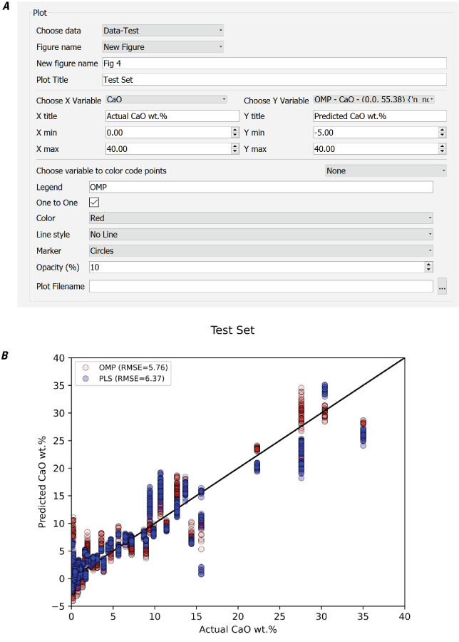
Screenshot and plot showing the PyHAT Plot module interface (A) and an example output plot (B) created using the “one to one” option to evaluate two different regression methods: orthogonal matching pursuit (OMP) and partial least squares (PLS). The root mean squared error (RMSE) is given for each regression. wt. %, weight percent.
Plot Spectra
The Plot Spectra module (fig. 23) allows the user to plot rows of data, typically spectra or similar (for example, peak areas, model coefficients, and so on). As with the Plot module, the user selects a dataset and specifies whether to create a new figure or plot additional data onto an existing figure. If creating a new figure, the axis titles and ranges may be specified. If plotting on an existing figure, these values are already set and are fixed.
The user then selects the x variable for the plot. The options for x variable are drawn from the top-level column names in the specified dataset (meta, comp, or wvl, as shown in fig. 1). After specifying the x variable, the range of x values is automatically set to span the full range of values for that variable. The user may adjust this range to create a plot that is zoomed in on a certain subset of the spectrum. The x-axis title defaults to the name of the x variable selected but may be edited by the user.
Next, the user chooses the column that contains the unique identifier that will be used to choose which row to plot (for example, Target Type from fig. 1). The choices in this drop-down list are drawn from the second-level column names in the dataset selected (Target Name, Target Type, Spectrum ID, and so on in fig. 1). When a column is chosen, the “Choose Rows” list box is populated with all the entries from that column. For example, it is common for a dataset to contain a metadata column containing target names or observation identifications that can be used to identify a spectrum, so the user would choose the “Target Name” column and then select the target desired from the “Choose Rows” list (for example, Olivine or Basalt from fig. 1). As with the x variable, when a row is selected, the y-axis range is automatically set to the minimum and maximum values from the spectrum but may be customized. The y-axis title is specified by the user.
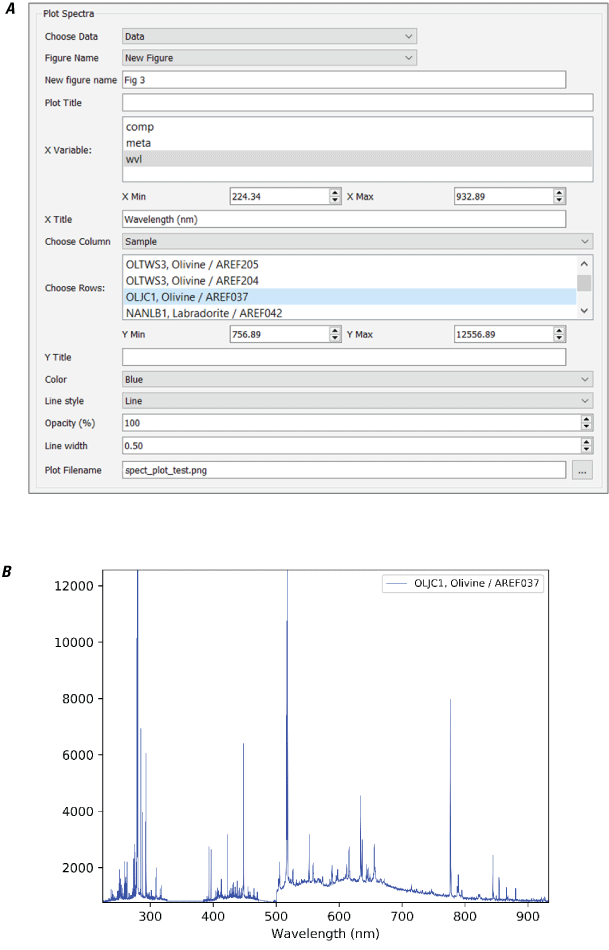
Screenshot of the PyHAT Plot Spectra module interface (A) and an example spectrum plot (B). Y-axis is in instrument counts. nm, nanometer.
The user may also choose the color of the line to plot and the line style (solid, dashed, dotted, and so on), opacity, and width. The legend for the plot will automatically use the text from the selected row to identify the line being plotted. Finally, the user may specify the file name.
Plot ICA/PCA
The Plot ICA/PCA module is used to visualize both the scores and loadings resulting from PCA or ICA dimensionality reduction (fig. 24). The user selects the dataset and the dimensionality reduction method of interest. The x and y variable lists are then populated with the names of the scores columns resulting from the selected dimensionality reduction. After selecting which scores to plot on the x- and y-axes, the user may choose to color code the points based on the value of a column from the dataset. This can aid in interpreting the scores by visually linking the points to values, such as composition. Finally, the user can specify a file name for the plot.
When run, the module creates a figure that has a scatterplot on the left showing the scores selected and two plots on the right showing the loadings used to calculate the scores as a function of wavelength (fig. 24).
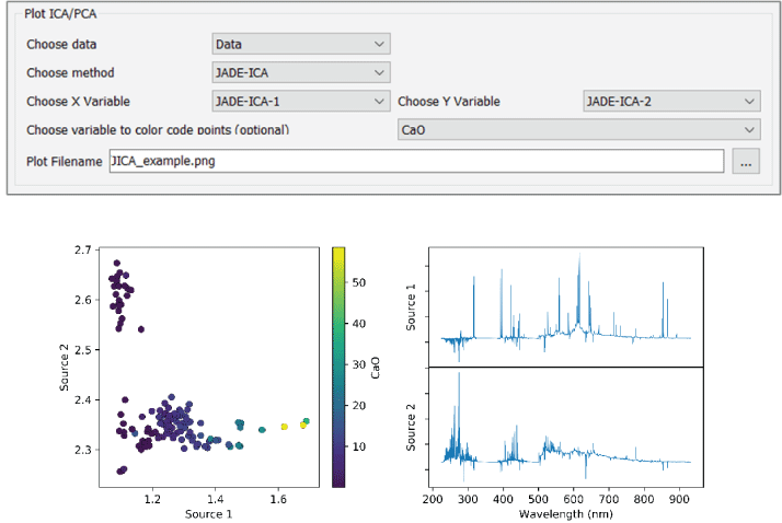
Screenshot of the PyHAT Plot ICA/PCA module interface (A) and an example of output plots (B). Plots show the independent component analysis (ICA) results, color coded by CaO concentration, in weight percent. Investigation of the source 1 loading plot and the color coding in the scatterplot both indicate that source 1 is correlated with CaO—in other words, as CaO increases, so does source 1. nm, nanometer.
Buttons
Several buttons along the bottom of the GUI (fig. 25) can be used to run or manipulate the modules in a workflow. The progress bar above these buttons will flash when a calculation is in progress and show as 100 percent when the calculation is complete. The “Re-run” button allows the user to rerun a module. When modules in the workflow are run, they are disabled (grayed out) and cannot be edited and rerun. Clicking the re-run button will reenable the last disabled module in the workflow. By clicking multiple times, multiple modules may be reenabled. Once reenabled, parameters may be modified, and the workflow may be run again. This is particularly useful when plotting, allowing the user to adjust the plotting parameters and create additional figures.
The “Stop” button stops the execution of the script. This functionality is useful if the workflow is running through a long calculation, such as cross validation, and the user wishes to abort the calculation; for example, if the user realizes that a parameter was not set correctly.
The “Insert After” list allows the user to insert a module into the workflow between preexisting (but not yet run) modules. This can be useful if the user wishes to add a preprocessing step into an existing workflow without having to delete subsequent modules. After a module has been inserted at the specified location, the insertion location is reset to the end of the workflow.
The “Delete” list allows the user to delete modules from the workflow. Only modules that are not disabled (grayed out) can be deleted.
The “OK” button runs the workflow. If new modules have been added after a previous run of the workflow, the workflow will run beginning with the first module that is not disabled (grayed out).
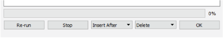
Screenshot showing buttons at the bottom of the PyHAT graphical user interface.
Examples
The following steps, split into several workflows for simplicity, represent the typical procedure for developing and applying a regression model using LIBS data. Although these do not cover every capability of the GUI, these serve as an instructive starting point for users. For users comfortable with running Python scripts directly rather than with a GUI, the PyHAT repository contains several additional examples demonstrating how to work with data from CRISM, M3, the Kaguya Spectral Profiler, and SuperCam.
Preprocessing Workflow
The preprocessing workflow begins, as all PyHAT workflows do, by specifying the output folder, followed by loading a dataset from a CSV file. This example uses spectra provided in the repository (libpyhat/data_sets/LIBS/lab_data_example.csv). Once loaded, baseline removal is applied using the airPLS algorithm (fig. 26).
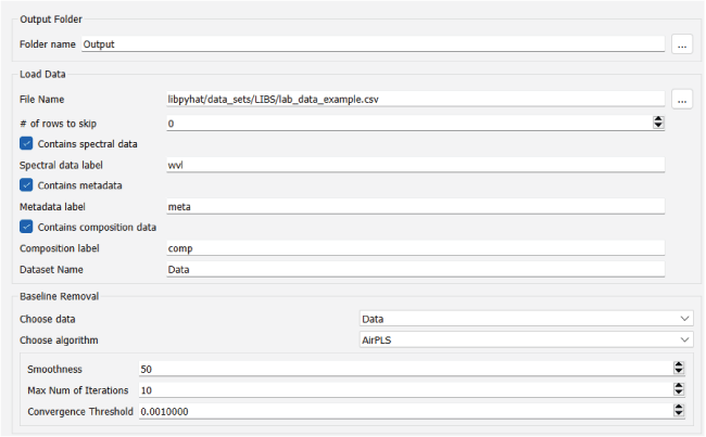
Screenshot showing the PyHAT preprocessing workflow step of loading the dataset and applying baseline removal.
To see how well baseline removal did, we then plot the original spectrum and the baseline identified by the (fig. 27). If desired, additional baseline removal steps that use different parameters or algorithms can be performed on the original dataset and plotted in a similar manner to determine the best choice for the dataset. For the purposes of this example, this tuning process is not included, and the default airPLS settings are used.
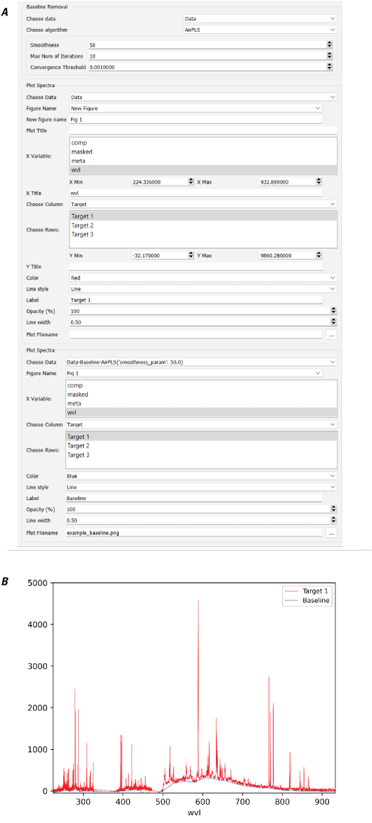
Screenshot and plot showing the PyHAT preprocessing workflow step of baseline removal. A, Screenshot showing how to run the adaptive iteratively reweighted penalized least squares (airPLS) baseline removal algorithm and plot the results. B, Plot of an original spectrum (red) and its airPLS-derived baseline (blue) generated by the module. Wavelength (wvl) plotted in nanometers.
Dimensionality Reduction Workflow
In this example, we use the SuperCam spectral library, which is available for download at https://pds-geosciences.wustl.edu/m2020/urn-nasa-pds-mars2020_supercam/calibration_supercam/libs_spectral_library_reference.csv. These data have already had baseline removal applied as part of the SuperCam data processing pipeline. These data have also had wavelength shifts applied, which we do not want to use in this example, so the first step after loading the data is to use the Remove Rows module to remove all rows with shift values other than 0 (fig. 28). Note that because this is a large dataset, the Remove Rows module takes some time to load – be patient! We next normalize the spectra so that each sums to one.
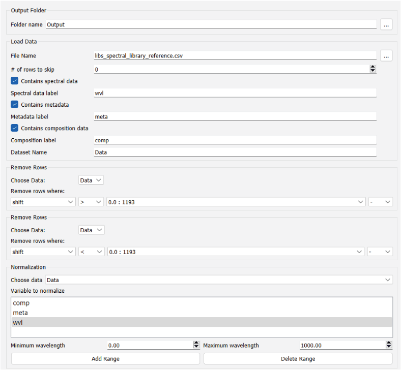
Screenshot showing the PyHAT preprocessing workflow steps of removing rows and normalizing a dataset prior to performing principal component analysis.
We then use the PCA dimensionality reduction step and visualize the scores and loadings for the first two principal components, which are color coded by the known total calcium oxide (CaO) concentration in each sample (fig. 29).
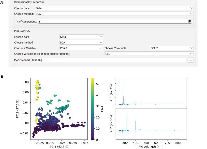
Screenshot and plots showing dimensionality reduction. A, Screenshot showing the user interface. Dimensionality reduction is done using principal component analysis (PCA). B, Plots showing PCA scores and loadings. Scores are color coded by total calcium oxide (CaO) content (in weight percent [wt.%]), showing that principal component 2 (PC2) has a strong positive correlation with CaO content. %, percent; nm, nanometer.
Cross Validation Workflow
When training a regression model, cross validation should be used to tune the parameters of the algorithms of interest to determine the optimal settings. This workflow begins by loading the preprocessed data from the previous workflow. The data are then stratified on the variable for which the regression model is trained—SiO2 abundance in this example (fig. 30).
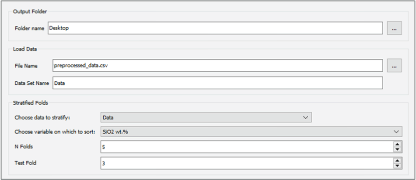
Screenshot showing the PyHAT cross-validation workflow step of loading the preprocessed data and sorting them into stratified folds based on SiO2 content to create a training set and a test set.
Next, cross validation is performed, which requires choosing a group of algorithms and hyperparameter values for evaluation (fig. 31). For the purposes of this simple example, the OLS and PLS regression algorithms are compared. In practice, testing additional regression algorithms would be more thorough. However, note that running cross validation with all the available regression algorithms and doing so over their many hyperparameters can be time consuming, particularly if local regression is included. Therefore, the user should determine how extensive of a cross-validation routine is required for their purposes.
Screenshot showing the PyHAT regression cross-validation workflow. Cross validation is used to compare different regression methods and choose the optimal parameters for a given method.
When cross validation is finished, the results are exported to a CSV file (fig. 32). The lowest RMSECV for OLS in the file is listed as 6.54 weight percent, whereas PLS achieves lower RMSECV in several cases. The lowest RMSECV is not necessarily the optimal choice for PLS, since using too many components can result in an overspecialized model that performs poorly on novel data. To choose the best model, the RMSECV versus number of components for PLS can be plotted (fig. 33). The best model is where the plot forms an elbow, and additional components do not significantly improve the RMSECV. In this case, the optimal number of components is seven.
Screenshot showing the PyHAT cross-validation workflow steps of saving cross-validation results to a file (A) and plotting root mean squared error of cross validation (RMSECV) versus the number of components to help optimize the partial least squares (PLS) regression (B).
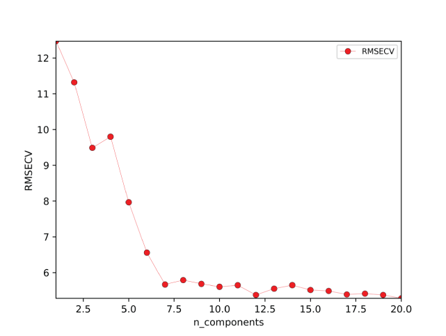
Plot of root mean squared error of cross validation (RMSECV) versus number of components generated by the PyHAT modules shown in figure 32. The optimal number of components is seven, above which there is no significant decrease in RMSECV.
Blended submodels get better results than a single PLS model can achieve alone, so this cross-validation workflow can be completed two more times, changing the range of compositions used for cross validation to 0–60 and 50–100 weight percent. These models are optimized with seven and eight components, respectively.
Regression Training and Prediction Workflow
In this example workflow, the results from cross validation are used to train the regression models, optimize the blending process, and then predict the test set. First, preprocessed data need to be loaded and the stratified folds method selected to separate the training and test data.
Regression models are then trained (fig. 34), using the parameters determined by cross validation, and those models are used to predict the train and test set compositions (fig. 35).
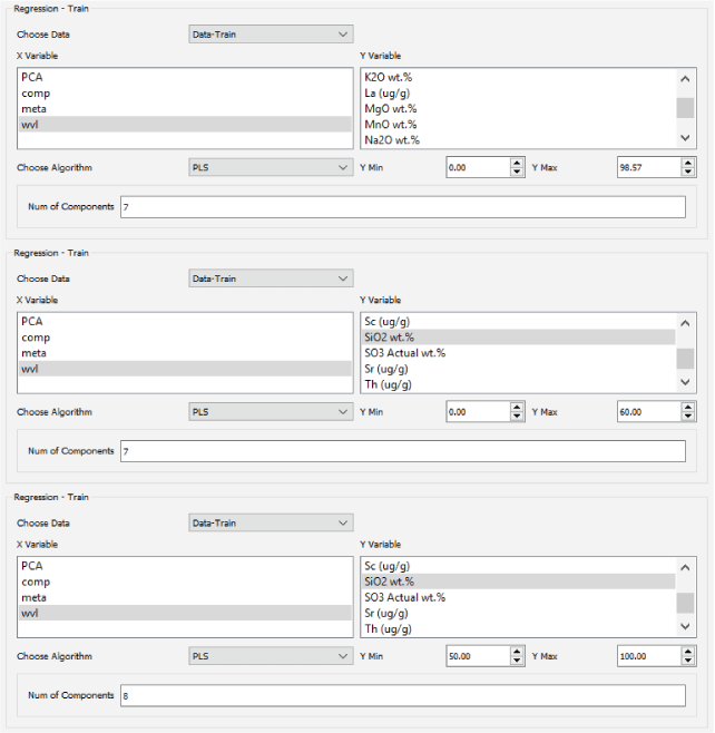
Screenshot showing the PyHAT regression workflow step of training three partial least squares (PLS) regression models for SiO2 content. The first one is trained on spectra from targets spanning 0 to 100 weight percent (wt. %), the second is trained on the 0 to 60 weight percent range, and the third is trained on the 50 to 100 weight percent range. The number of components were determined by cross validation in the previous workflow.
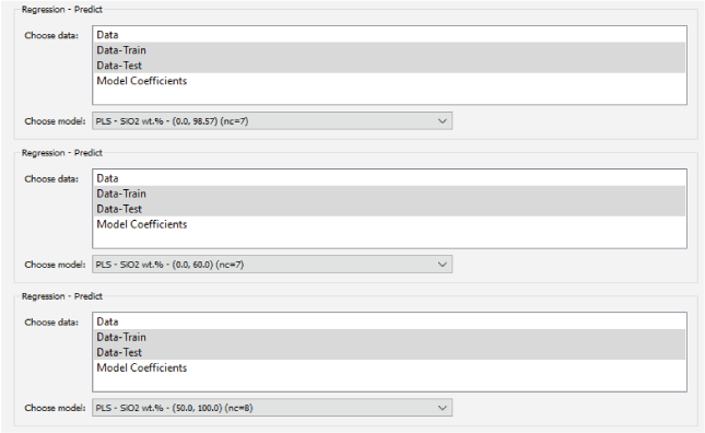
Screenshot showing the PyHAT regression workflow step of using each SiO2 model to predict the SiO2 content of the training and test sets.
Once predictions are complete, the Blended Submodel Predictions module can be used with the training set predictions first (fig. 36). The 0–100 weight percent PLS model in this case is used as the reference model, the 0–60 weight percent model as the low model, and the 50–100 weight percent model as the high model. When optimizing the blending by comparing the results with the known SiO2 compositions, the lowest RMSE is achieved with a blending range from 27.71 to 64.16 weight percent. This means, for reference model predictions below 27.71 weight percent, the predictions from the low model will be used, above 64.16 weight percent the high model will be used, and in between the results will be blended using a linear weighted sum. Next, the same blending range is applied to the test set predictions, and the test set results are plotted against the known compositions to evaluate the accuracy of the final blended predictions (fig. 37).
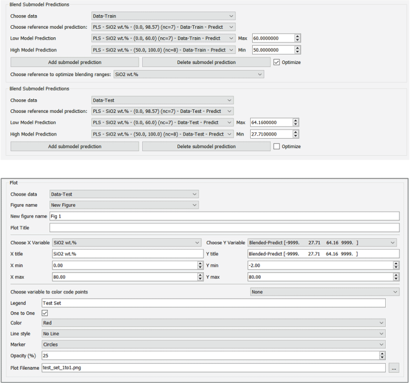
Screenshots showing the PyHAT regression workflow steps of optimizing the submodel blending predictions and plotting the results. A, Submodel blending uses the training set predictions and then uses the optimal blending range for the test set predictions. B, Plot the blended test set predictions versus the true SiO2 values to evaluate the model performance.
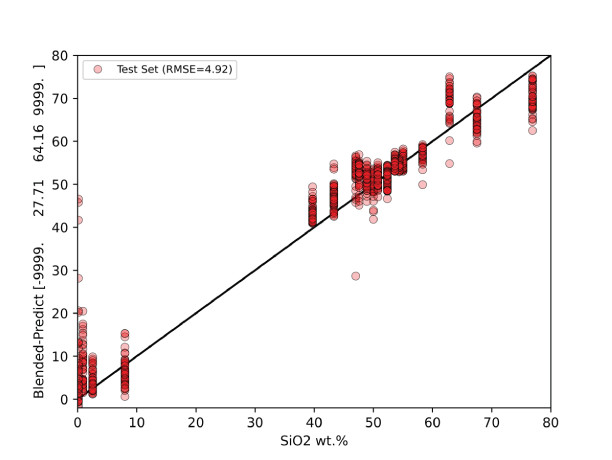
Plot of blended test set predictions versus actual SiO2 concentration (in weight percent [wt.%]) generated by the PyHAT module shown in figure 36. Black line shows the one-to-one ratio.
Endmember Identification and Spectral Unmixing Workflow
PyHAT is not only for analysis of planetary datasets, it is useful for terrestrial remote sensing as well. In this example, endmembers are identified from a subset of the Salinas Scene dataset (see the Endmember Identification section above for more information about the dataset). Note that because there can be considerable spectral variability for a single ground truth (for example, lettuce), the endmember identification algorithm may not always identify unique ground truths. Instead, it may include spectral extremes of a single ground truth (for example, old and young lettuce crop).
First, the Salinas Scene dataset multicolumn test file “labeled_Salinas_testfile.csv,” provided as part of the PyHAT repository, is loaded and named. For this example, the spectra are also normalized using the normalize functionality in the preprocessing drop-down menu. The variable to normalize is set to “wvl.” The spectra are normalized from a minimum wavelength of 0 to a maximum of 2,500 (the actual wavelengths of the data are 360 to 2,500 nm). Using the data drop-down menu, “Identify endmembers” is selected. For this example, the PPI algorithm is used, and the number of endmembers is set to three. When endmember identification is run, a column is added to the dataset.
To unmix the composite Salinas spectra, the “Unmixing” option in the preprocessing drop-down menu is used. In this case, the same dataset for both the data to unmix and the endmembers is used because the endmembers were added to the dataset. The unmixing method used in this example is FCLS. The “Normalize” box is left unchecked because the spectra were normalized in the previous steps. Figure 38 shows a screenshot of the unmixing workflow, and figure 39 shows a plot of the three identified endmember spectra.
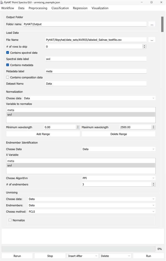
Screenshot of the PyHAT endmember identification and unmixing workflow.
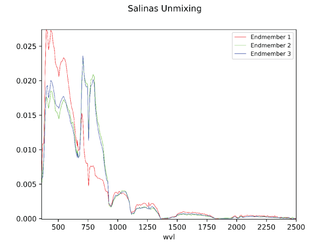
Plot of endmembers identified in the Salinas spectra example. Wavelength (wvl) plotted in nanometers; y-axis is normalized spectral intensity.
Conclusion
This user guide describes the features available in the Python Hyperspectral Analysis Tool (PyHAT) and its graphical user interface (GUI). The PyHAT interface makes data processing, visualization, and machine learning techniques accessible to a wide variety of users and allows for sharing of workflows. The back end PyHAT library can be readily imported in Python applications when greater flexibility is required than that provided by the GUI. Ultimately, this allows PyHAT to serve as a standalone tool or part of an analysis pipeline, increasing the ease of adoption by a broad technical community.
PyHAT development is ongoing, and new capabilities are constantly being considered, incorporated, and tested. This user guide refers to the PyHAT 0.1.2 release. We welcome community input on PyHAT and its GUI via the code.usgs.gov repository or email (contact the authors at rbanderson@usgs.gov, tgabriel@usgs.gov, or ianeece@usgs.gov).
References Cited
Anderson, R.B., Clegg, S.M., Frydenvang, J., Wiens, R.C., McLennan, S., Morris, R.V., Ehlmann, B.L., and Dyar, M.D., 2017, Improved accuracy in quantitative laser-induced breakdown spectroscopy using sub-models: Spectrochimica Acta Part B—Atomic Spectroscopy, v. 129, p. 49–57, https://doi.org/10.1016/j.sab.2016.12.002.
Anderson, R.B., Forni, O., Cousin, A., Wiens, R.C., Clegg, S.M., Frydenvang, J., Gabriel, T.S.J., Ollila, A., Schröder, S., Beyssac, O., Gibbons, E., Vogt, D.S., Clavé, E., Manrique, J-A., Legett, C., IV, Pilleri, P., Newell, R.T., Sarrao, J., Maurice, S., Arana, G., Benzerara, K., Bernardi, P., Bernard, S., Bousquet, B., Brown, A.J., Alvarez-Llamas, C., Chide, B., Cloutis, E., Comellas, J., Connell, S., Dehouck, E., Delapp, D.M., Essunfeld, A., Fabre, C., Fouchet, T., Garcia-Florentino, C., García-Gómez, L., Gasda, P., Gasnault, O., Hausrath, E.M., Lanza, N.L., Laserna, J., Lasue, J., Lopez, G., Madariaga, J.M., Mandon, L., Mangold, N., Meslin, P.-Y., Nelson, A.E., Newson, H., Reyes-Newell, A.L., Robinson, S., Rull, F., Sharma, S., Simon, J.I., Sobron, P., Torre Fernandez, I., Udry, A., Venhaus, D., McLennan, S.M., Morris, R.V., and Ehlmann, B., 2022, Post-landing major element quantification using SuperCam laser induced breakdown spectroscopy: Spectrochimica Acta Part B—Atomic Spectroscopy, v. 188, article 106347, https://doi.org/10.1016/j.sab.2021.106347.
Bai, L., Lin, H., Sun, H., Zang, Z., and Mo, D., 2012, Remotely sensed percent tree cover mapping using support vector machine combined with autonomous endmember extraction: Physics Procedia, v. 33, p. 1702–1709, https://doi.org/10.1016/j.phpro.2012.05.274.
Bell, J., III, Farrand, W., Johnson, J., and Morris, R., 2002, Low abundance materials at the Mars Pathfinder landing site—An investigation using spectral mixture analysis and related techniques: Icarus, v. 158, p. 56–71, https://doi.org/10.1006/icar.2002.6865.
Benachir, D., Deville, Y., Hosseini, S., and Karoui, M., 2020, Blind unmixing of hyperspectral remote sensing data—A new geometrical method based on a two-source sparsity constraint: Remote Sensing, v. 12, no. 3198, p. 1–25, https://doi.org/10.3390/rs12193198.
Benkstein, K.D., Rogers, P.H., Montgomery, C.B., Jin, C., Raman, B., and Semancik, S., 2014, Analytical capabilities of chemiresistive microsensor arrays in a simulated Martian atmosphere: Sensors and Actuators B—Chemical, v. 197, p. 280–291, https://doi.org/10.1016/j.snb.2014.02.088.
Bertsekas, D.P., 2011, Incremental proximal methods for large scale convex optimization: Mathematical Programming, v. 129, p. 163–195, https://doi.org/10.1007/s10107-011-0472-0.
Bjorgan, A., and Randeberg, L., 2015, Real-time noise removal for line-scanning hyperspectral devices using a minimum noise fraction-based approach: Sensors, v. 15, p. 3362–3378, https://doi.org/10.3390/s150203362.
Boucher, T., Dyar, M.D., and Mahadevan, S., 2017, Proximal methods for calibration transfer: Journal of Chemometrics, v. 31, article no. e2877, https://doi.org/10.1002/cem.2877.
Bratsch, S., Epstein, H., Buchhorn, M., and Walker, D., 2016, Differentiating among four Arctic tundra plant communities at Ivotuk, Alaska using field spectroscopy: Remote Sensing, v. 8, no. 1, article no. 51, 17 p., https://doi.org/10.3390/rs8010051.
Breunig, M.M., Kriegel, H.-P., Ng, R.T., and Sander, J., 2000, LOF—Identifying density-based local outliers, in Proceedings of the SIGMOD/PODS00 ACM International Conference on Management of Data and Symposium on Principles of Database Systems, Dallas, Texas, May 15–18, 2000: New York, Association for Computing Machinery, p. 93–104.
Bue, B., Thompson, D., Sellar, R., Podest, E., Eastwood, M., Helmlinger, M., McCubbin, I., and Morgan, J., 2015, Leveraging in-scene spectra for vegetation species discrimination with MESMA-MDA: ISPRS Journal of Photogrammetry and Remote Sensing, v. 108, p. 33–48, https://doi.org/10.1016/j.isprsjprs.2015.06.001.
Cai, J-F., Candès, E.J., and Shen, Z., 2010, A singular value thresholding algorithm for matrix completion: Society for Industrial and Applied Mathematics Journal on Optimization, v. 20, p. 1956–1982, https://doi.org/10.1137/080738970.
Cai, T.T., and Wang, L., 2011, Orthogonal matching pursuit for sparse signal recovery with noise: Transactions on Information Theory, v. 57, p. 4680–4688, https://doi.org/10.1109/TIT.2011.2146090.
Calvino-Cancela, M., and Martin-Herrero, J., 2016, Spectral discrimination of vegetation classes in ice-free areas of Antarctica: Remote Sensing, v. 8, no. 10, article no. 856, 15 p., https://doi.org/10.3390/rs8100856.
Capizzi, G., and Masarotto, G., 2011, A least angle regression control chart for multidimensional data: Technometrics, v. 53, p. 285–296, https://doi.org/10.1198/TECH.2011.10027.
Casalino, G., and Gillis, N., 2017, Sequential dimensionality reduction for extracting localized features: Pattern Recognition, v. 63, p. 15–29, https://doi.org/10.1016/j.patcog.2016.09.006.
Ceamanos, X., Doute, S., Luo, B., Schmidt, F., Jouannic, G., and Chanussot, J., 2011, Intercomparison and validation of techniques for spectral unmixing of hyperspectral images—A planetary case study: Transactions on Geoscience and Remote Sensing, v. 49, no. 11, p. 4341–4358, https://doi.org/10.1109/TGRS.2011.2140377.
Chang, C., Chen, S., Li, H., Chen, H., and Wen, C., 2016, Comparative study and analysis among ATGP, VCA, and SGA for finding endmembers in hyperspectral imagery: Journal of Selected Topics in Applied Earth Observations and Remote Sensing, v. 9, no. 9, p. 4280–4306, https://doi.org/10.1109/JSTARS.2016.2555960.
Chang, C., Li, Y., and Wang, Y., 2017, Progressive band processing of fast iterative pixel purity index for finding endmembers: Geoscience and Remote Sensing Letters, v. 14, no. 9, p. 1464–1468, https://doi.org/10.1109/LGRS.2017.2710219.
Chang, C., and Plaza, A., 2006, A fast iterative algorithm for implementation of pixel purity index: Geoscience and Remote Sensing Letters, v. 3, no. 1, p. 63–67, https://doi.org/10.1109/LGRS.2005.856701.
Chang, C., and Wu, C., 2015, Design and development of iterative pixel purity index: Journal of Selected Topics in Applied Earth Observations and Remote Sensing, v. 8, no. 6, p. 2676–2695, https://doi.org/10.1109/JSTARS.2015.2403259.
Chen, J., Bing, Z., Mao, Z., Zhang, C., Bi, Z., and Yang, Z., 2018, Using geochemical data for prospecting target areas by the sequential maximum angle convex cone method in the Manzhouli area, China: Geochemical Journal, v. 52, p. 13–27, https://doi.org/10.2343/geochemj.2.0493.
Clegg, S.M., Frydenvang, J., Anderson, R.B., Vaniman, D.T., Gasda, P., Forni, O., Newsom, H., Blaney, D., and Wiens, R.C., 2020, Quantitative sulfur chemistry observed on diverse samples from sols 1800–2300 [abs.], in Lunar and Planetary Science Conference, 51st, The Woodlands, Texas, March 16–20, 2020, scientific program: Lunar and Planetary Institute and National Aeronautics and Space Administration, no. 2561, 2 p.
Clegg, S.M., Wiens, R.C., Anderson, R.B., Forni, O., Frydenvang, J., Lasue, J., Cousin, A., Payré, V., Boucher, T., Dyar, M.D., McLennan, S.M., Morris, R.V., Graff, T.G., Mertzman, S.A., Ehlmann, B.L., Belgacem, In., Newsom, H., Clark, B.C., Melikechi, N., Mezzacappa, A., McInroy, R.E., Martinez, R., Gasda, P., Gasnault, O., and Maurice, S., 2017, Recalibration of the Mars Science Laboratory ChemCam instrument with an expanded geochemical database: Spectrochimica Acta Part B—Atomic Spectroscopy, v. 129, p. 64–85, https://doi.org/10.1016/j.sab.2016.12.003.
Cobas, C.J., Bernstein, M.A., Martín-Pastor, M., and Tahoces, P.G., 2006, A new general-purpose fully automatic baseline-correction procedure for 1D and 2D NMR data: Journal of Magnetic Resonance, v. 183, p. 145–151, https://doi.org/10.1016/j.jmr.2006.07.013.
Cui, C., Li, Y., Liu, B., and Li, G., 2017, A new endmember preprocessing method for the hyperspectral unmixing of imagery containing marine oil spills: International Journal of Geo-Information, v. 6, no. 9, article no. 286, 21 p., https://doi.org/10.3390/ijgi6090286.
Das, P.K., and Seshasai, M.V.R., 2015, Multispectral sensor spectral resolution simulations for generation of hyperspectral vegetation indices from Hyperion data: Geocarto International, v. 30, no. 6, p. 686–700, https://doi.org/10.1080/10106049.2014.973065.
Dietrich, W., Rüdel, C.H., and Neumann, M., 1991, Fast and precise automatic baseline correction of one- and two-dimensional nmr spectra: Journal of Magnetic Resonance (1969), v. 91, p. 1–11, https://doi.org/10.1016/0022-2364(91)90402-F.
Douté, S., Schmitt, B., Langevin, Y., Bibring, J., Altieri, F., Bellucci, G., Gondet, B., Poulet, F., and MEX OMEGA team, 2007, South pole of Mars—Nature and composition of the icy terrains from Mars Express OMEGA observations: Planetary and Space Science, v. 55, p. 113–133, https://doi.org/10.1016/j.pss.2006.05.035.
Drugowitsch, J., 2019, Variational Bayesian inference for linear and logistic regression: ArXiv preprint server, arXiv:1310.5438 statistics, 28 p., accessed April 15, 2021, at https://arxiv.org/abs/1310.5438.
Efendi, A., and Effrihan, 2017, A simulation study on Bayesian Ridge Regression models for several collinearity levels, in International Conference and Workshop on Mathematical Analysis and its Applications, Malang, Indonesia, August 2–3, 2017: American Institute of Physics Conference Proceedings, v. 1913, article no. 020031, 6 p., https://doi.org/10.1063/1.5016665.
Ettabaa, K.S., and Ben Salem, M., 2018, Adaptive progressive band selection for dimensionality reduction in hyperspectral images: Journal of the Indian Society of Remote Sensing, v. 46, p. 157–167, https://doi.org/10.1007/s12524-017-0691-9.
Forni, O., Maurice, S., Gasnault, O., Wiens, R.C., Cousin, A., Clegg, S.M., Sirven, J.-B., and Lasue, J., 2013, Independent component analysis classification of laser induced breakdown spectroscopy spectra: Spectrochimica Acta Part B—Atomic Spectroscopy, v. 86, p. 31–41, https://doi.org/10.1016/j.sab.2013.05.003.
Ghamisi, P., Yokoya, N., Li, J., Liao, W., Liu, S., Plaza, J., Rasti, B., and Plaza, A., 2017, Advances in hyperspectral image and signal processing—A comprehensive overview of the state of the art: Geoscience and Remote Sensing Magazine, v. 5, no. 4, p. 37–78, https://doi.org/10.1109/MGRS.2017.2762087.
Giguere, S., Carey, C., Dyar, M.D., Boucher, T.F., Parente, M., Tague, T.J., and Mahadevan, S., 2015, Baseline removal in LIBS and FTIR spectroscopy; Optimization techniques [abs.], in Lunar and Planetary Science Conference, 46th, The Woodlands, Texas, March 16–20, 2015, scientific program: Lunar and Planetary Institute and National Aeronautics and Space Administration, no. 2775, 2 p.
Gillis, N., and Plemmons, R., 2013, Sparse nonnegative matrix underapproximation and its application to hyperspectral image analysis: Linear Algebra and its Applications, v. 438, no. 10, p. 3991–4007, http://doi.org/10.1016/j.laa.2012.04.033.
Gilmore, M.S., Thompson, D.R., Anderson, L.J., Karamzadeh, N., Mandrake, L., and Castaño, R., 2011, Superpixel segmentation for analysis of hyperspectral data sets, with application to Compact Reconnaissance Imaging Spectrometer for Mars data, Moon Mineralogy Mapper data, and Ariadnes Chaos, Mars: Journal of Geophysical Research, v. 116, n. E07001, p. 1–19, https://doi.org/10.1029/2010JE003763.
Gohler, D., Fischer, B., and Meissner, S., 2017, In-ovo sexing of 14-day-old chicken embryos by pattern analysis in hyperspectral images (VIS/NIR spectra)—A non-destructive method for layer lines with gender-specific down feather color: Poultry Science, v. 96, no. p. 1–4, https://doi.org/10.3382/ps/pew282.
González, C., Bernabe, S., Mozos, D., and Plaza, A., 2016, FPGA implementation of an algorithm for automatically detecting targets in remotely sensed hyperspectral images: Journal of Selected Topics in Applied Earth Observations and Remote Sensing, v. 9, no. 9, p. 4334–4343, https://doi.org/10.1109/JSTARS.2015.2504427.
Graps, A., 1995, An introduction to wavelets: Computational Science and Engineering, v. 2, no. 2, p. 50–61, https://doi.org/10.1109/99.388960.
Hamzeh, S., Naseri, A., AlaviPanah, S., Bartholomeus, H., and Herold, M., 2016, Assessing the accuracy of hyperspectral and multispectral satellite imagery for categorical and quantitative mapping of salinity stress in sugarcane fields: International Journal of Applied Earth Observation and Geoinformation, v. 52, p. 412–421, https://doi.org/10.1016/j.jag.2016.06.024.
Heinz, D.C. and Chang, C.I., 2001, Fully constrained least squares linear spectral mixture analysis method for material quantification in hyperspectral imagery: Transactions on Geoscience and Remote Sensing, v. 39, no. 3, p. 529–545, https://doi.org/10.1109/36.911111.
Heylen, R., 2018, Rob Heylen Research code: self-published by author, accessed December 7, 2022, at https://web.archive.org/web/20221207130159/https://sites.google.com/site/robheylenresearch/code.
Hirose, Y., and Komaki, F., 2010, An extension of least angle regression based on the information geometry of dually flat spaces: Journal of Computational and Graphical Statistics, v. 19, p. 1007–1023, https://doi.org/10.1198/jcgs.2010.09064.
Houborg, R., McCabe, M., Angel, Y., and Middleton, E., 2016, Detection of chlorophyll and leaf area index dynamics from sub-weekly hyperspectral imagery, in Proceedings of the Society of Photo-Optical Instrumentation Engineers Remote Sensing for Agriculture, Ecosystems, and Hydrology, XVIII, Edinburgh, U.K., 2016, 11 p., https://doi.org/10.1117/12.2241345.
Huang, X., and Zhang, L., 2008, An adaptive mean-shift analysis approach for object extraction and classification from urban hyperspectral imagery: Transactions on Geoscience and Remote Sensing, v. 46, no. 12, p. 4173–4185, https://doi.org/10.1109/TGRS.2008.2002577.
Hyvärinen, A., and Oja, E., 2000, Independent component analysis—Algorithms and applications: Neural Networks, v. 13, p. 411–430, https://doi.org/10.1016/S0893-6080(00)00026-5.
Kajfosz, J., and Kwiatek, W.M., 1987, Nonpolynomial approximation of background in X-ray spectra: Nuclear Instruments and Methods in Physics Research Section B—Beam Interactions with Materials and Atoms, v. 22, p. 78–81, https://doi.org/10.1016/0168-583X(87)90298-9.
Kale, K., Solankar, M., Nalawade, D., Dhumal, R., and Gite, H., 2017, A research review on hyperspectral data processing and analysis algorithms: Proceedings of the National Academy of Sciences, India, Section A, v. 87, no. 4, p. 541–555, https://doi.org/10.1007/s40010-017-0433-y.
Khajehrayeni, F., and Ghassemian, H., 2021, A linear hyperspectral unmixing method by means of autoencoder networks: International Journal of Remote Sensing, v. 42, no. 7, p. 2517–2531, https://doi.org/10.1080/01431161.2020.1854893.
Kodikara, G., Ray, P., Chauhan, P., and Chatterjee, R., 2016, Spectral mapping of morphological features on the moon with MGM and SAM: International Journal of Applied Earth Observation and Geoinformation, v. 44, p. 31–41, https://doi.org/10.1016/j.jag.2015.07.003.
Kumar, U., Ganguly, S., Nemani, R., Raja, K., Milesi, C., Sinha, R., Michaelis, A., Votava, P., Hashimoto, H., Li, S., Wang, W., Kalia, S., and Gayaka., S., 2017, Exploring subpixel learning algorithms for estimating global land cover fractions from satellite data using high performance computing: Remote Sensing, v. 9, no. 1105, p. 1–25, https://doi.org/10.3390/rs9111105.
Lee, Y., Clarke, M., Tokumasu, F., Lesoine, J., Allen, D., Chang, R., Litorja, M., and Hwang, J., 2012, Absorption-based hyperspectral imaging and analysis of single erythrocytes: Journal of Selected Topics in Quantum Electronics, v. 18, p. 1–10, https://doi.org/10.1109/JSTQE.2011.2164239.
Liland, K.H., Almøy, T., and Mevik, B-H., 2010, Optimal choice of baseline correction for multivariate calibration of spectra: Applied Spectroscopy, v. 64, p. 1007–1016, https://doi.org/10.1366/000370210792434350.
Liu, F.T., Ting, K.M., and Zhou, Z-H., 2012, Isolation-based anomaly detection: Association for Computing Machinery Transactions on Knowledge Discovery from Data, v. 6, p. 1–39, https://doi.org/10.1145/2133360.2133363.
Liu, R., Du, B., and Zhang, L., 2016a, Hyperspectral unmixing via double abundance characteristics constraints based NMF: Remote Sensing, v. 8, no. 464, p. 2–23, https://doi.org/10.3390/rs8060464.
Liu, Y., Glotch, T., Scudder, N., Kraner, M., Condus, T., Arvidson, R., Guinness, E., Wolff, M., and Smith, M., 2016b, End-member identification and spectral mixture analysis of CRISM hyperspectral data—A case study on southwest Melas Chasma, Mars: Journal of Geophysical Research—Planets, v. 121, p. 2004–2036.
Lu, D., Batistella, M., Moran, E., and Mausel, P., 2004, Application of spectral mixture analysis to Amazonian land-use and land-cover classification: International Journal of Remote Sensing, v. 25, no. 23, p. 5345–5358, https://doi.org/10.1080/01431160412331269733.
Lu, C-J., Lee, T-S., and Chiu, C-C., 2009, Financial time series forecasting using independent component analysis and support vector regression: Decision Support Systems, v. 47, p. 115–125, https://doi.org/10.1016/j.dss.2009.02.001.
Luo, H., Tang, Y., and Yang, L., 2015, Subspace learning via local probability distribution for hyperspectral image classification: Mathematical Problems in Engineering, v. 2015, p. 1–17, http://doi.org/10.1155/2015/145136.
Marcinkowska-Ochtyra, A., Zagajewski, B., Ochtyra, A., Jarocińska, A., Wojtuń, B., Rogass, C., Mielke, C., and Lavender, S., 2017, Subalpine and alpine vegetation classification based on hyperspectral APEX and simulated EnMAP images: International Journal of Remote Sensing, v. 38, no. 7, p. 1839–1864, https://doi.org/10.1080/01431161.2016.1274447.
Maurice, S., Wiens, R.C., Saccoccio, M., Barraclough, B., Gasnault, O., Forni, O., Mangold, N., Baratoux, D., Bender, S., Berger, G., Benardin, J., Berthé, M., Bridges, N., Blaney, D., Bouyé, M., Caïs, P., Clark, B., Clegg, S., Cousin, A., Cremers, D., Cros, A., DeFlores, L., Derycke, C., Dingler, B., Dromart, G., Dubois, B., Dupieux, M., Durand, E., d’Uston, L., Fabre, C., Faure, B., Gaboriaud, A., Gharsa, T., Herkenhoff, K., Kan, E., Kirkland, L., Kouach, D., Lacour, J-L., Langevin, Y., Lasue, J., Le Mouélic, S., Lescure, M., Lewin, E., Limonadi, D., Manhès, G., Mauchien, P., McKay, C., Meslin, P-Y., Michel, Y., Miller, E., Newsom, H.E., Orttner, G., Paillet, A., Parés, L., Parot, Y., Pérez, R., Pinet, P., Poitrasson, F., Quertier, B., Sallé, B., Sotin, C., Sautter, V., Séran, H., Simmonds, J.J., Sirven, J-B., Stiglich, R., Striebig, N., Thocaven, J-J., Toplis, M.J., and Vaniman, D., 2012, The ChemCam instrument suite on the Mars Science Laboratory (MSL) rover—Science objectives and mast unit description: Space Science Reviews, v. 170, p. 95–166, https://doi.org/10.1007/s11214-012-9912-2.
Molan, Y., Refahi, D., and Tarashti, A., 2014, Mineral mapping in the Maherabad area, eastern Iran, using the HyMap remote sensing data: International Journal of Applied Earth Observation and Geoinformation, v. 27, p. 117–127, https://doi.org/10.1016/j.jag.2013.09.014.
Morgan, M.F., Seelos, F.P., and Murchie, S.L., 2017, The CRISM Analysis Toolkit (CAT)—Overview and recent updates [abs.], in Planetary Data Workshop, 3rd, Flagstaff, Arizona, June 12–15: Planetary Geologic Mappers, 2 p., accessed October 5, 2013, at https://www.hou.usra.edu/meetings/planetdata2017/pdf/7121.pdf.
Murchie, S., Arvidson, R., Bedini, P., Beisser, K., Bibring, J-P., Bishop, J., Boldt, J., Cavender, P., Choo, T., Clancy, R.T., Darlington, E.H., Des Marais, D., Espiritu, R., Fort, D., Green, R., Guinness, E., Hayes, J., Hash, C., Heffernan, K., Hemmler, J., Heyler, G., Humm, D., Hutcheson, J., Izenberg, N., Lee, R., Less, J., Lohr, D., Malaret, E., Martin, T., McGovern, J.A., McGuire, P., Morris, R., Mustartd, J., Pelkey, S., Rhodes, E., Robinson, M., Roush, R., Schaefer, E., Seagrave, G., Seelos, F., Silverglate, P., Slavney, S., Smith, M., Shyong, W-J., Strohbehn, K., Taylor, H., Thompson, P., Tossman, B., Wirzburger, M., and Wolff, M., 2007, Compact Reconnaissance Imaging Spectrometer for Mars (CRISM) on Mars Reconnaissance Orbiter (MRO): Journal of Geophysical Research, v. 112, article no. E05S03, https://doi.org/10.1029/2006JE002682.
NV5 Geospatial Solutions, 2014, Why is constrained unmixing usually a bad idea?: NV5 Geospatial Solutions, Inc., Technical Support web page, accessed February 27, 2025, at https://www.nv5geospatialsoftware.com/Support/Self-Help-Tools/Help-Articles/ArtMID/10216/ArticleID/19704/1630.
pandas development team, 2023, pandas-dev/pandas—Pandas (ver. 2.1.0): Zenodo, https://doi.org/10.5281/zenodo.8301632.
Parente, M., Bishop, J., and Bell, J., III, 2009, Spectral unmixing for mineral identification in pancam images of soils in Gusev crater, Mars: Icarus, v. 203, p. 421–436, https://doi.org/10.1016/j.icarus.2009.04.029.
Pedregosa, F., Varoquaux, G., Gramfort, A., Michel, V., Thirion, B., Grisel, O., Blondel, M., Prettenhofer, P., Weiss, R., Dubourg, V., Vanderplas, J., Passos, A., Cournapeau, D., Brucher, M., Perrot, M., and Duchesnay, E., 2011, Scikit-learn—Machine learning in Python: Journal of Machine Learning Research, v. 12, p. 2825–2830.
Pieters, C.M., Boardman, J., Buratti, B., Chatterjee, A., Clark, R., Glavich, T., Green, R., Head, J., III, Isaacson, P., Malaret, E., McCord, T., Mustard, J., Petro, N., Runyon, C., Staid, M., Sunshine, J., Taylor, L., Tompkins, S., Varanasi, P., and White, M., 2009, The Moon Mineralogy Mapper (M3) on Chandrayaan-1: Current Science, v. 96, 6 p.
Pu, R., Xu, B., and Gong, P., 2003, Oakwood crown closure estimation by unmixing Landsat TM data: International Journal of Remote Sensing, v. 24, no. 22, p. 4422–4445, https://doi.org/10.1080/0143116031000095989.
Qu, L., Han, W., Lin, H., Zhu, Y., and Zhang, L., 2014, Estimating vegetation fraction using hyperspectral pixel unmixing method—A case study of a karst area in China: Journal of Selected Topics in Applied Earth Observations and Remote Sensing, v. 1, no. 11, p. 1–7, https://doi.org/10.1109/JSTARS.2014.2361253.
Remon, A., Sanchez, S., Bernabe, S., Quintana-Orti, E., and Plaza, A., 2013, Performance versus energy consumption of hyperspectral unmixing algorithms on multi-core platforms: EURASIP Journal of Advances in Signal Processing, v. 2013, no. 68, p. 1–15, https://doi.org/10.1186/1687-6180-2013-68.
Rogers, A., and Aharonson, O., 2008, Mineralogical composition of sands in Meridiani Planum determined from Mars Exploration Rover data and comparison to orbital measurements: Journal of Geophysical Research, v. 113, article no. E06S14, p. 1–19, https://doi.org/10.1029/2007JE002995.
Shahdoosti, H., and Mirzapour, F., 2017, Spectral–spatial feature extraction using orthogonal linear discriminant analysis for classification of hyperspectral data: European Journal of Remote Sensing, v. 50, no. 1, p. 111–124, https://doi.org/10.1080/22797254.2017.1279821.
Shao, Z., Zhou, W., Cheng, Q., Diao, C., Zhang, L., 2015, An effective hyperspectral image retrieval method using integrated spectral and textural features: Sensor Review, v. 35, no. 3, p. 274–281, https://doi.org/10.1108/SR-10-2014-0716.
Singh, K., and Ramakrishnan, D., 2017, A comparative study of signal transformation techniques in automated spectral unmixing of infrared spectra for remote sensing applications: International Journal of Remote Sensing, v. 38, no. 5, p. 1235–1257, https://doi.org/10.1080/01431161.2017.1280625.
Therian, C., 2018, Welcome to the PySptools Documentation—Tools for hyperspectral imaging (ver. 0.15.0): self-published by author, https://pysptools.sourceforge.io.
Thompson, D., Mandrake, L., Gilmore, M., and Castano, R., 2010, Superpixel endmember detection: Transactions on Geoscience and Remote Sensing, v. 48, no. 11, p. 4023–4033, https://doi.org/10.1109/TGRS.2010.2070802.
Viviano, C.E., Seelos, F.P., Murchie, S.L., Kahn, E.G., Seelos, K.D., Taylor, H.W., Taylor, K., Ehlmann, B.L., Wiseman, S.M., Mustard, J.F., and Morgan, M.F., 2014, Revised CRISM spectral parameters and summary products based on the currently detected mineral diversity on Mars: Journal of Geophysical Research—Planets, v. 119, no. 6, p. 1403–1431, https://doi.org/10.1002/2014JE004627.
Voss, S., Magni, P., Dadour, I., and Nansen, C., 2017, Reflectance-based determination of age and species of blowfly puparia: International Journal of Legal Medicine, v. 131, no. 1, p. 263–274, https://doi.org/10.1007/s00414-016-1458-5.
van der Walt, S., Colbert, S.C., and Varoquaux, G., 2011, The NumPy array—A structure for efficient numerical computation: Computing in Science and Engineering, v. 13, p. 22–30, https://doi.org/10.1109/MCSE.2011.37.
Wang, D., and Lu, W-Z., 2006, Interval estimation of urban ozone level and selection of influential factors by employing automatic relevance determination model: Chemosphere, v. 62, no. 10, p. 1600–1611, https://doi.org/10.1016/j.chemosphere.2005.06.047.
Wang, G., Ding, Q., and Hou, Z., 2008, Independent component analysis and its applications in signal processing for analytical chemistry: Trends in Analytical Chemistry, v. 27, p. 368–376, https://doi.org/10.1016/j.trac.2008.01.009.
Wang, Y., Veltkamp, D.J., and Kowalski, B.R., 1991, Multivariate instrument standardization: Analytical Chemistry, v. 63, p. 2750–2756, https://doi.org/10.1021/ac00023a016.
Wen, J., Fowler, J., He, M., Zhao, Y., Deng, C., and Menon, V., 2016, Orthogonal nonnegative matrix factorization combining multiple features for spectral-spatial dimensionality reduction of hyperspectral imagery: Transactions on Geoscience and Remote Sensing, v. 54, no. 7, p. 4272–4286, https://doi.org/10.1109/TGRS.2016.2539154.
Wen, J., Tian, Z., Liu, X., and Lin, W., 2013, Neighborhood preserving orthogonal PNMF feature extraction for hyperspectral image classification: Journal of Selected Topics in Applied Earth Observations and Remote Sensing, v. 6, no. 2, p. 759–768, https://doi.org/10.1109/JSTARS.2012.2210276.
Wiens, R.C., Maurice, S., Barraclough, B., Saccoccio, M., Barkley, W.C., Bell, J.F., III, Bender, S., Bernardin, J., Blaney, D., Blank, J., Bouyé, M., Bridges, N., Bultman, N., Caïs, P., Clanton, R.C., Clark, B., Clegg, S., Cousin, A., Cremers, D., Cros, A., DeFlores, L., Delapp, D., Dingler, R., d’Uston, C., Dyar, M.D., Elliott, T., Enemark, D., Fabre, C., Flores, M., Forni, O., Gasnault, O., Hale, T., Hays, C., Herkenhoff, K., Kan, E., Kirkland, L., Douach, D., Landis, D., Langevin, Y., Lanza, N., LaRocca, F., Lasue, J., Latino, J., Limonadi, D., Lindensmith, C., Little, C., Mangold, N., Manhès, G., Mauchien, P., McKay, C., Miller, E., Mooney, J., Morris, R.V., Morrison, L., Nelson, T., Newsom, H., Ollila, A., Ott, M., Pares, L., Pérez, R., Poitrasson, F., Provost, C., Reiter, J.W., Roberts, T., Romero, F., Sautter, V., Salazar, S., Simmonds, J.J., Stiglich, R., Storms, S., Striebig, N., Thocaven, J-J., Trujillo, T., Ulibarri, M., Vaniman, D., Warner, N., Waterbury, R., Whitaker, R., Witt, J., and Wong-Swanson, B., 2012, The ChemCam instrument suite on the Mars Science Laboratory (MSL) rover—Body unit and combined system tests: Space Science Reviews, v. 170, p. 167–227, https://doi.org/10.1007/s11214-012-9902-4.
Wiens, R.C., Maurice, S., Lasue, J., Forni, O., Anderson, R.B., Clegg, S., Bender, S., Blaney, D., Barraclough, B.L., Cousin, A., Deflores, L., Delapp, D., Dyar, M.D., Fabre, C., Gasnault, O., Lanza, N., Mazoyer, J., Melikechi, N., Meslin, P-Y., Newsom, H., Ollila, A., Perez, R., Tokar, R.L., and Vaniman, D., 2013, Pre-flight calibration and initial data processing for the ChemCam laser-induced breakdown spectroscopy instrument on the Mars Science Laboratory rover: Spectrochimica Acta Part B—Atomic Spectroscopy, v. 82, p. 1–27, https://doi.org/10.1016/j.sab.2013.02.003.
Wu, C.-H., Ho, J.-M., and Lee, D.T., 2004, Travel-time prediction with support vector regression: Transactions on Intelligent Transportation Systems, v. 5, p. 276–281, https://doi.org/10.1109/TITS.2004.837813.
Wu, X., Huang, B., Plaza, A., Li, Y., and Wu, C., 2014, Real-time implementation of the pixel purity index algorithm for endmember identification on GPUs: Geoscience and Remote Sensing Letters, v. 11, no. 5, p. 955–959, https://doi.org/10.1109/LGRS.2013.2283214.
Ye, Z., Bai, L., and Nian, Y., 2017, Decision fusion for hyperspectral image classification based on multiple features and locality-preserving analysis: European Journal of Remote Sensing, v. 50, no. 1, p. 166–178, https://doi.org/10.1080/22797254.2017.1299556.
Yu, P-S., Chen, S-T., and Chang, I-F., 2006, Support vector regression for real-time flood stage forecasting: Journal of Hydrology, v. 328, p. 704–716, https://doi.org/10.1016/j.jhydrol.2006.01.021.
Zazi, L., Boutaleb, A., and Guettouche, M., 2017, Identification and mapping of clay minerals in the region of Djebel Meni (Northwestern Algeria) using hyperspectral imaging, EO-1 Hyperion sensor: Arab Journal of Geosciences, v. 10, article no. 252, 10 p., https://doi.org/10.1007/s12517-017-3015-z.
Zhang, C., Qin, Q., Chen, L., Wang, N., Zhao, S., and Hui, J., 2015b, Rapid determination of coalbed methane exploration target region utilizing hyperspectral remote sensing: International Journal of Coal Geology, v. 150–151, p. 19–34, https://doi.org/10.1016/j.coal.2015.07.010.
Zhang, X., Nansen, C., Aryamanesh, N., Yan, G., and Boussaid, F., 2015a, Importance of spatial and spectral data reduction in the detection of internal defects in food products: Applied Spectroscopy, v. 69, no. 4, p. 1–8, https://doi.org/10.1366/14-07672.
Zhang, Y., Wang, X., Balzter, H., Qiu, B., and Cheng, J., 2019, Directional and zonal analysis of urban thermal environmental change in Fuzhou as an indicator of urban landscape transformation: Remote Sensing, v. 11, no. 23, article no. 2810, 19 p., https://doi.org/10.3390/rs11232810.
Zhang, Z-M., Chen, S., and Liang, Y-Z., 2010, Baseline correction using adaptive iteratively reweighted penalized least squares: Analyst, v. 135, p. 1138–1146, https://doi.org/10.1039/B922045C.
Zhao, C., Zhao, G., Qi, B., and Li, X., 2015, Reduced near border set for endmember extraction: Optik, v. 126, p. 4424–4431, https://doi.org/10.1016/j.ijleo.2015.08.114.
Zheng, K., Zhang, X., Iqbal, J., Fan, W., Wu, T., Du, Y., and Liang, Y., 2014, Calibration transfer of near-infrared spectra for extraction of informative components from spectra with canonical correlation analysis: Journal of Chemometrics, v. 28, p. 773–784, https://doi.org/10.1002/cem.2637.
Zhu, F., and Honeine, P., 2016, Biobjective nonnegative matrix factorization—Linear versus kernel-based models: Transactions on Geoscience and Remote Sensing, v. 54, no. 7, p. 4012–4022, https://doi.org/10.1109/TGRS.2016.2535298.
Abbreviations
airPLS
adaptive iteratively reweighted penalized least squares
ALS
asymmetric least squares
ARD
automatic relevance determination
ATGP
automatic target generation process
AVIRIS
Airborne Visible/Infrared Imaging Spectrometer
BRR
Bayesian ridge regression
CAT
CRISM Analysis Toolkit
CCA
canonical correlation analysis
CCS
cleaned calibrated spectra
CRISM
Compact Reconnaissance Imaging Spectrometer for Mars
CSV
comma-separated values
DS
direct standardization
FABC
fully automatic baseline correction
FCLS
fully constrained least squares
FIPPI
fast iterative pixel purity index
FTIR
Fourier transform infrared spectroscopy
GBM
Generalized bilinear model
GDAL
Geospatial Data Abstraction Library
GUI
graphical user interface
HTML
HyperText Markup Language
ICA
independent component analysis
IDL
Interactive Data Language
JADE
joint approximate diagonalization of eigenmatrices
JSON
JavaScript Object Notation
KK
Kajfosz-Kwiatek
LARS
least angle regression
LASSO
least absolute shrinkage and selection operator
LDA
linear discriminant analysis
LFDA
local Fisher’s discriminant analysis
LIBS
laser-induced breakdown spectroscopy
LLE
locally linear embedding
LPP
locality preserving projection
M3
Moon Mineralogy Mapper
MNF
minimum noise fraction
NASA
National Aeronautics and Space Administration
NIPALS
nonlinear iterative partial least squares
nm
nanometer
NNLS
nonnegative least squares
NNMF
nonnegative matrix factorization
OLS
ordinary least squares
OMP
orthogonal matching pursuit
PCA
principal component analysis
PDS
piecewise direct standardization
PLS
partial least squares
PNG
portable network graphic
PPI
pixel purity index
PyHAT
Python Hyperspectral Analysis Toolkit
RMSE
root mean squared error
RMSEC
root mean squared error of calibration
RMSECV
root mean squared error of cross validation
RMSEP
root mean squared error of prediction
SMACC
sequential maximum angle convex cone
SQLSP
sequential least squares programming
SVD
singular value decomposition
SVM
support vector machine
SVR
support vector regression
TES
Thermal Emission Spectrometer
t-SNE
t-distributed stochastic neighbor embedding
UCLS
unconstrained least squares
USGS
U.S. Geological Survey
Disclaimers
Any use of trade, firm, or product names is for descriptive purposes only and does not imply endorsement by the U.S. Government.
Although this information product, for the most part, is in the public domain, it also may contain copyrighted materials as noted in the text. Permission to reproduce copyrighted items must be secured from the copyright owner.
Suggested Citation
Anderson, R.B., Aneece, I.P., and Gabriel, T.S.J., 2025, Python Hyperspectral Analysis Tool (PyHAT) user guide: U.S. Geological Survey Open-File Report 2025–1038, 59 p., https://doi.org/10.3133/ofr20251038.
ISSN: 2331-1258 (online)
| Publication type | Report |
|---|---|
| Publication Subtype | USGS Numbered Series |
| Title | Python Hyperspectral Analysis Tool (PyHAT) user guide |
| Series title | Open-File Report |
| Series number | 2025-1038 |
| DOI | 10.3133/ofr20251038 |
| Publication Date | August 22, 2025 |
| Year Published | 2025 |
| Language | English |
| Publisher | U.S. Geological Survey |
| Publisher location | Reston, VA |
| Contributing office(s) | Astrogeology Science Center |
| Description | xi, 59 p. |
| Online Only (Y/N) | Y |