Three-dimensional seismic velocity model for the Cascadia Subduction Zone with shallow soils and topography, version 1.7

Erin A. Wirth; Alex R. Grant; Ian P. Stone; William J. Stephenson; Arthur D. Frankel

doi:10.3133/ofr20251045

Three-Dimensional Seismic Velocity Model for the Cascadia Subduction Zone with Shallow Soils and Topography, Version 1.7

Open-File Report 2025-1045

By: Erin A. Wirth, Alex R. Grant, Ian P. Stone, William J. Stephenson, and Arthur D. Frankel

https://doi.org/10.3133/ofr20251045

Metrics

Web analytics dashboard Metrics definitions

Links

Document: Report (4.4 MB pdf) , HTML , XML
Data Release: USGS data release - Data for A 3-D Seismic Velocity Model for Cascadia with Shallow Soils & Topography, Version 1.7
Superseded Publications:

P- and S-wave velocity models incorporating the Cascadia subduction zone for 3D earthquake ground motion simulations, Version 1.6—Update for Open-File Report 2007–1348(2017)

Download citation as: RIS | Dublin Core

Acknowledgments

We thank the workshop attendees from the 2019 “Future Strategies for the 3D Cascadia Seismic Velocity Model” for conversations that helped motivate these updates. We also thank Nasser Marafi (Moody’s RMS) for conversations that contributed to the development of this work, as well as Audrey Dunham (U.S. Geological Survey), Evan Hirakawa (U.S. Geological Survey), and Valerie Sahakian (University of Oregon) for helpful comments that improved this report. Seismic data from the 2001 magnitude 6.8 Nisqually earthquake were downloaded from the EarthScope Consortium Web Services.

Abstract

The U.S. Geological Survey’s seismic velocity model for the Cascadia Subduction Zone provides P- and S-wave velocity (V_P and V_S, respectively) information from 40.2° to 50.0° N. latitude and −129.0° to −121.0° W. longitude, and is used to support a variety of research topics, including three-dimensional (3D) earthquake simulations and seismic hazard assessment in the Pacific Northwest. This report describes an update to the previous version (v) 1.6 of the 3D seismic velocity model for the Cascadia Subduction Zone. This new model (herein referred to as v1.7) contains more detailed near-surface structure for improved earthquake ground motion modeling. Updated features include the addition of a new shallow soil velocity model in the top 200 meters and the option of adding user-specified topography. Although v1.6 of the Cascadia seismic velocity model has a minimum V_S of 600 meters per second (m/s), the new model (v1.7) has a minimum V_S of approximately 40 m/s. Overall, this update will allow for more accurate ground motion estimates from 3D simulations of scenario earthquakes in the Cascadia Subduction Zone region.

Introduction

The U.S. Geological Survey’s (USGS) seismic velocity model for the Cascadia Subduction Zone includes three-dimensional (3D) P- (V_P) and S-wave (V_S) velocity information spanning the region from northern California to southern British Columbia, Canada, from 40.2° to 50.0° N. latitude and −129.0° to −121.0° W. longitude (Stephenson, 2007; Stephenson and others, 2017). In this report, we present an update to model version (v) 1.6 of Stephenson and others (2017). The previous versions of the Cascadia seismic velocity model (CVM) are flat at the surface (did not include topography) and had a minimum shear-wave velocity (V_S_min) of 600 meters per second (m/s). Yet, it has been shown that low seismic wave speeds and topography have the potential to substantially affect the amplitude of earthquake ground shaking (for example, Frankel and others, 2002; Stone and others, 2022). This newly updated model (herein referred to as model v1.7) contains updates to the near-surface structure (less than or equal to [≤] 1,200 meters [m]), which will allow for more accurate waveform modeling of scenario earthquakes in the Pacific Northwest. Model v1.7 includes the addition of a shallow soil velocity model (V_Smin approximately [~] 40 m/s) in the top few hundred meters. A supplementary Python function for adding user-specified topography and bathymetry can be applied as needed using the software release that accompanies this report (Wirth and Stone, 2024; also available on GitLab at https://code.usgs.gov/esc/cvm_topo). A data release also accompanies this report and contains the V_P and V_S data for model v1.7 (Wirth and others, 2025).

Motivation for Updating Near-Surface Structure

Regional-scale seismic velocity models are commonly used to produce 3D earthquake simulations and estimates of ground shaking during an earthquake (Graves and Aagaard, 2011; Taborda and Bielak, 2013; Moschetti and others, 2017; Razafindrakoto and others, 2018; Rodgers and others, 2020). They can also be used as starting models for geophysical inversions of Earth structure (Fichtner and others, 2013; Nguyen and others, 2021) and for high-resolution earthquake relocation and moment tensor inversion studies (Lomax and others, 2001; Eberhart-Phillips and others, 2010; Hauksson and others, 2012; Wang and Zhan, 2020). Numerous previous studies have used v1.6 of the CVM for 3D ground motion simulations of earthquakes on the Cascadia Subduction Zone (Frankel and others, 2018; Wirth and others, 2018b; Roten and others, 2019), in the Puget Sound region (Stone and others, 2022, 2023), and for defining regional subsurface properties for seismic hazard estimates (Petersen and others, 2020).

The accurate characterization of shallow-site effects is important for estimating earthquake hazard, as shallow Earth structure has the potential to affect the amplitude and frequency content of earthquake ground shaking. However, v1.6 of the CVM did not include topography and had a minimum shear-wave velocity of 600 m/s (that is, approximately the shear-wave velocity of a soft rock site). It has been shown through observations and modeling that topography has the potential to substantially change the amplitude of ground shaking. For example, Hartzell and others (2013) examined earthquake records around mountainous topography in San Jose, California, and observed amplification factors of 3–4 at the resonance frequency (0.5–1 hertz [Hz]) of a nearby ridge relative to a site at the ridge base. Similarly, Stone and others (2022) found that topographic amplification could increase the amplitude of short period (less than [<] 2 seconds [s]) ground motions by 25–35 percent when comparing earthquake simulations with and without topography.

Shallow-site effects also substantially influence strong ground motions (Frankel and others, 2002). In particular, shallow soft (V_S <180 m/s) and stiff (180 < V_S < 360 m/s) soils will affect earthquake ground shaking and seismic hazard estimates, particularly frequencies greater than (>) 0.5 Hz. During the 2001 magnitude (M) 6.8 Nisqually, Washington, earthquake, Frankel and others (2002) observed increasing site amplification with decreasing shear-wave velocity measured in the top 30 m (V_S30). At 1 Hz, soft soil sites were amplified by factors of 3–7 compared to a nearby soft rock site. These areas of stronger site amplification correlated with the most substantial damage to buildings and evidence of liquefaction from the Nisqually earthquake.

Due to the lack of observational recordings from large earthquakes in the Pacific Northwest, numerical simulations of hypothetical earthquakes are often used to estimate seismic hazard. However, these earthquake simulations have typically had a relatively high minimum shear-wave velocity (~600 m/s; Frankel and others, 2018; Wirth and others, 2018b), which requires the application of subsequent site adjustment factors to estimate ground shaking at sites with V_S30 <600 m/s. Wirth and others (2020) calculated site-specific amplification factors using equivalent linear analysis, which were used to adjust estimated shaking from ground motion simulations of Cascadia Subduction Zone earthquakes. For peak ground acceleration, stiff soil sites generally required site amplification factors of ~1–1.25. As advances in high-performance computing make large-scale 3D numerical simulations more tractable, directly modeling wave propagation in Earth materials with very low shear-wave velocity becomes increasingly possible. This highlights the importance of a regional-scale seismic velocity model with relatively low P- and S-wave velocities.

Development and Integration of a Near-Surface Model

In this report, we describe the development and addition of a shallow soil model to the 3D CVM. The shallow soil model characterizes the top few hundred meters and is based on regional V_S30 estimates and compilations of measured soil profiles throughout the Pacific Northwest. We also provide an option for adding user-specified topography using supplementary Python code (Wirth and Stone, 2024; https://code.usgs.gov/esc/cvm_topo). The new CVM (v1.7) includes V_P and V_S in netCDF4 format, with the following horizontal (dx=dy) and vertical (dz) spacing:

• dx=dy=200 m and dz=10 m at 0–100 m depths
• dx=dy=200 m and dz=100 m at 200–1,200 m depths
• dx=dy=dz=300 m at 1,500–9,900 m depths
• dx=dy=dz=900 m at 10,800–59,400 m depths

Shallow Soil Velocity Model

To develop the soil velocity model, we use three separate datasets of measured V_S(z) profiles in the Pacific Northwest:

1. A compilation of profiles collected over several years and using a variety of methods in Oregon, Washington, and southern British Columbia (Ahdi and others, 2017).
2. Profiles collected by the Washington Department of Natural Resources (WA DNR) since 2017, as part of their school seismic safety project (Washington Geological Survey, 2021). These profiles are located throughout Washington and northernmost Oregon and are based on active source multi-channel analysis of surface waves (MASW) and passive source microtremor array measurements (MAM; West and others, 2019). This dataset was screened to remove all duplicates of profiles contained in the Ahdi and others (2017) dataset.
3. High-resolution V_S profiles in the Tacoma and Seattle, Washington, regions collected by Friedman Alvarez and others (2024) using microtremor array data.

The measured profiles are divided into four categories based on their locations: Willamette Valley, fill and alluvium, Puget Lowland, and “other” sites (fig. 1, table 1). We discarded any profiles from the Fraser River delta south of Vancouver, British Columbia, included in the Ahdi and others (2017) dataset, which are slow to deeper depths (V_S=1.0 km/s at depths >200 m) and not necessarily representative of the shallow velocity gradients that we are interested in for the broader Pacific Northwest (Marafi and others, 2021).

Alttext 1: The Cascadia seismic velocity model spans from northern California, through
western Washington and Oregon, to southern British Columbia. The Cascadia Subduction
Zone (the boundary between the Juan de Fuca Plate and North America Plate) runs north
to south in the Pacific Ocean off the west coast. — Figure 1.
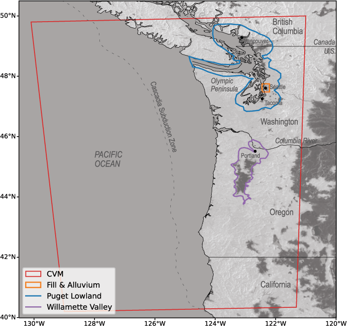
Map of the Cascadia region extending along the west coast of the United States and southern British Columbia, Canada. The red box denotes the extent of the three-dimensional (3D) Cascadia seismic velocity model (CVM). The regional divisions used to develop the shallow soil velocity model (that is, Willamette Valley, fill and alluvium, and Puget Lowland) are also shown; any sites outside of these regional divisions are designated as “other” sites. The approximate boundary between the subducting Juan de Fuca Plate and overriding North America Plate is indicated by the dashed line (https://earthquake.usgs.gov/learn/plate-boundaries.kmz; last accessed August 2, 2024). Base map is “Stamen terrain” from Stadia Maps (https://www.stadiamaps.com; last accessed June 26, 2024).

For each region, measured profiles are used in a regression to determine generalized equations for V_S as a function of depth and V_S30, using the functional form:

V s (z) = A + B z + C \ln z + D

(1)

A = A_{0} + A_{1} * V_{S 30}

(2)

B = B_{0} * [{V_{S 30} * V}_{S z = 100}] + B_{1} * V_{S 30} + B_{2} * V_{S z = 100}

(3)

C = C_{0} + C_{1} * V_{S 30} + C_{2} * V_{S z = 100}

(4)

where

z: is depth in meters,
V_Sz: ₁₀₀ is V_S at z=100 m in the Stephenson and others (2017) model,
A, B, and C: are solved for, as part of the regression, and
D: is an additional offset term used for Puget Lowland sites only (described below).

All constant terms (that is, A_0–1, B_0–2, and C_0–2) are given in table 1. The natural log term in equation 1 controls the curvature of the profile at shallow depths (approximately <50 m), and the linear depth term controls V_S at greater depths. For the Willamette Valley region, WA DNR profiles were withheld from model fitting as a test dataset. For Puget Lowland and “other” sites, all profiles, including those from the WA DNR compilation, were included for greater spatial coverage and data density.

For the glacial sediments of the Puget Lowland, all considered Puget Lowland-area profiles were used to determine the coefficients in A and C, which determine V_S at the surface (z=0) and the log-curvature of the profile (at depths of approximately <50 m), respectively. However, using the Ahdi and others (2017) profiles, which typically only extended to 20–50 m, to constrain the linear term (B) yielded generalized V_S profiles that increased too rapidly at depth. Therefore, only the Friedman Alvarez and others (2024) profiles, which typically extend a few hundred meters, were used to fit the linear term B that controls the shear wave velocity at depths beyond ~30–50 m. For these Puget Lowland sites, we also solve for an additional offset term (D in equation 1) as a function of V_S30 by comparing the V_S values of the input (measured data) and output (generalized profiles). This results in an additional term that lowers V_S(z) by $(- 0.32 * {V s}_{30} + 58)$ , or approximately 50 m/s for a site with V_S30 ~350 m/s.

For fill and alluvium sites in the greater Seattle area, a linear generalized profile was used with the following functional form:

V_{S} (z) = A + B * z

(5)

A = A_{0} + A_{1} * V_{S 30}

(6)

B = B_{0} + B_{1} * V_{S 30}

(7)

where A and B were again solved for in the regression. This was determined to provide a better fit to measured values compared to the generalized form that included log-curvature. For further details on the development of the generalized profiles, we refer the reader to Grant and others (in press). Details regarding how the shallow soil velocity model is assigned to specific point locations and merged with the deeper Stephenson and others (2017) CVM are discussed in the following sections.

Table 1.

Regionally dependent constants for generalized soil velocity profiles in the Cascadia Subduction Zone region, as used in seismic velocity model (CVM) version 1.7.

^{[All constant terms (that is, A_0–1, B_0–2, and C_0–2) are solved for as part of the regression. D is an additional offset term used for Puget Lowland sites only. For each region,
we indicate the number of measured shear-wave velocity (V_S) profiles used in the regression. No., number; —, not used in the regression. For
location of the regions, refer to fig. 1]}

Table 1. Regionally dependent constants for generalized soil velocity profiles in the Cascadia Subduction Zone region, as used in seismic velocity model (CVM) version 1.7.
Region	No. of profiles	A₀	A₁	B₀	B₁	B₂	C₀	C₁	C₂	D
Puget Lowland	267	−47.807	0.695	−1.462e-5	1.514e-2	4.932e-3	-3.581e1	1.951e-1	3.058e-2	$- 0.32 * {V s}_{30} + 58$
Fill and alluvium¹	93	−19.108	0.772	1.972	0.015	—	—	—	—	—
Willamette Valley	94	111.147	0.126	−7.618e-6	1.844e-2	2.058e-3	-8.976e1	3.636e-1	1.190e-2	0
Other	182	−0.641	0.357	−2.417e-6	4.306e-3	1.996e-3	-8.810e1	3.239e-1	1.984e-2	0

¹

Seattle area only.

Selection of a V_S30 Map

We use the V_S30 map developed by Geyin and Maurer (2023) as input to the generic soil velocity profiles. This V_S30 map was developed for the 50 U.S. States and Puerto Rico using machine learning on a variety of geospatial data and has been shown to perform well at predicting subsurface conditions where measured data are available. Because this V_S30 map does not extend into southern British Columbia, we revert to the USGS’s slope-based V_S30 map in Canada (Wald and Allen, 2007). Refer to the “Summary and Future Directions” section for additional discussion about available V_S30 maps.

Sites Within the Puget Lowland

A generic soil profile was developed for Puget Lowland sites using 267 measured profiles. We defined the Puget Lowland as the region of Washington State and southern British Columbia with Quaternary deposits in v1.6 of the CVM, which is based on multiple studies in the Puget Sound area (Jones, 1996; Johnson and others, 1999; Frankel and Stephenson, 2000; Mosher and Johnson, 2000). We cross-referenced these points with a geologic map (Ludington and others, 2005; Cui and others, 2017) to verify that they were on a mapped Quaternary unit. Sites located underwater (that is, beneath the Puget Sound), but within the Puget Lowland, were grouped into this category and assigned a V_S30 value of 600 m/s.

Puget Lowland grid points are assigned V_S values as a function of depth and V_S30 based on equation 1. For each site location, once the V_S value from equation 1 exceeded the V_S from model v1.6 at depth, V_S values reverted to the v1.6 values for all greater depths (fig. 2). This transition between seismic velocities defined by the new soil velocity model and model v1.6 typically occurred at ~100–200 m depth (fig. 3). For sites where the thickness of the Quaternary sediment layer is 100 m in model v1.6, we force the V_S transition to occur at 100 m, in order to preserve the shape of the Quaternary-Tertiary sediment boundary. V_P values were assigned by assuming a V_P/V_S ratio of 2.5 in Quaternary sediment (V_S ≤900 m/s) and gradually transitioning to a V_P/V_S ratio of 2.0 in Tertiary sediment (V_S ³1,000 m/s).

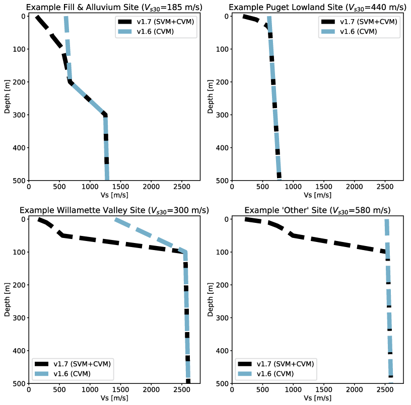
Alttext 2: New shear wave velocity profiles from this study exhibit lower seismic
velocities in the upper 50-200 meters compared to the original profiles. — Figure 2.
Examples of shear-wave velocity (V_S) profiles from single sites located within distinct regions of the Cascadia Subduction Zone region. Original V_S profiles from version (v) 1.6 of the Cascadia seismic velocity model (CVM; Stephenson and others, 2017) are shown in blue, whereas the updated V_S profiles (v1.7), which include a shallow soil-velocity model (SVM), are shown in black. For a map of regions, refer to figure 1. m, meter; m/s, meter per second; V_S30, time-averaged shear-wave velocity to a depth of 30 m.

Sites on Fill and Alluvium in Seattle

A generalized V_S profile for Holocene fill and alluvium sites in the greater Seattle area was developed using 93 measured profiles (table 1). The lateral extent and depth of fill and alluvium in Seattle was based on estimates from borehole data (for example, Frankel and others, 2007, their fig. 26). The maximum depth extent of alluvial material in this region is ~70 m. Model grid points that were on land and fell within the mapped extent of Holocene fill and alluvium were assigned a V_S value based on equation 5. All sites were assigned a V_S30 value of 185 m/s, based on the average measured V_S30 for sites located on fill and alluvium in the Seattle region. At grid points deeper than the estimated depth of fill and alluvium, V_S values reverted to the values that would have been assigned to a typical Puget Lowland site. This resulted in changes to the curvature of the V_S profile at the base of the fill and alluvium layer (fig. 2). P-wave velocity (V_P) values were set using an assumed V_P/V_S ratio of 2.5.

Sites Within the Willamette Valley

A separate generalized soil velocity profile was developed and applied to sites within the Willamette Valley, Oregon, which is based on 94 measured profiles and the functional form in equation 1. We manually defined the extent of the Willamette Valley geologic region based on the mapped location of outburst flood deposits within the Willamette River valley and their confluence with the Columbia River using the Oregon Department of Geology and Mineral Industries data (Burns and Coe, 2012; fig. 1). We followed the V_S values from the generalized profile until they exceeded the V_S from model v1.6 or a maximum of 50 m depth, at which point we linearly interpolated back to the v1.6 values at 100 m depth (figs. 2 and 3). (We note that due to the lack of basin-scale structures in the Willamette Valley and Portland area in model v1.6, this merging of the v1.7 and v1.6 models is likely not realistic.) We applied V_P/V_S ratios between 2.0 and 2.2 for all sites. In addition, we also set a minimum V_S30 cutoff (200 m/s) because the measured profiles used to develop the generic V_S profile are not representative of sites with lower V_S30 values.

Other Sites

Sites that were not within any of the predefined regions described above were assigned the V_S values defined by equation 1 and using 182 measured profiles (table 1). These were typically rock or hard rock sites. At these locations, the generalized soil profile was used to define V_S values to a depth of 50 m. This cutoff depth was chosen because very few measured profiles from rock sites extend beyond 50 m depth. At greater depths, V_S values were defined by linearly interpolating between 50 m depth (V_S defined by eq. 1) and 100 m depth (V_S defined by model v1.6). At a few sites where Quaternary sediment may have extended too deep in the v1.6 model, such that V_S values at 100 m depth were not consistent with that of a rock site, V_S values were linearly interpolated between 50 and 200 m depth. Beyond the maximum interpolated depth, the v1.6 values were not modified. We set a minimum V_S30 of 300 m/s for all sites, again based on the applicability of the available measured soil profiles. V_P was calculated using a V_P/V_S ratio of 2.2. We note that all sites west of the Pacific Coast were not modified and retain their original v1.6 model values. Water was assigned V_P and V_S values equal to −999.

Alttext 3: The thickness of the new soil velocity model ranges from approximately
50–200 meters, with most sites having a thickness of 100 meters. The Portland area
has velocities less than 50 meters, and the northern Olympic Peninsula has velocities
of just over 200 meters. — Figure 3.
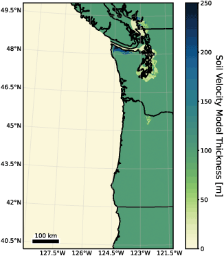
Map showing the thickness of the soil velocity model in the Cascadia Subduction Zone region. At most sites, the soil velocity model is less than or equal to 100 meters (m) thick. Exceptions include areas where model version 1.6 of the Cascadia seismic velocity model (CVM; Stephenson and others, 2017) has shear-wave velocity (V_S) values that are likely too fast (the greater Portland area) or too slow (northern Olympic Peninsula) in the top hundreds of meters given the estimated time-averaged shear-wave velocity to a depth of 30 m (V_S30) or mapped geologic unit, respectively.

Adding Topography and Bathymetry

We do not explicitly provide a version of our updated CVM v1.7 with topography in this publication due to file size limitations, given the high elevations contained within our model extent (>4,000 m) and fine-scale vertical spacing needed to describe the soil velocity model. However, we include a Python function in the software release (Wirth and Stone, 2024; https://code.usgs.gov/esc/cvm_topo) that allows users to add topography to the model using our recommended rules for adding or removing material. Adding topography as a final, user-initiated step also provides more flexibility in selecting topography files that accurately capture the region of interest at the desired resolution. Here, we describe the process by which topography may be added using the Python script. We note that topography and bathymetry may only be added to locations east of the Pacific Coast, because offshore bathymetry is already included in the flat-layered version (v1.6 and v1.7) of the CVM.

We accommodate topography and inland bathymetry by shifting the top portion of a one-dimensional (1D) velocity column beneath each site, such that it aligns with the topographic surface. Simultaneously, we either add (for sites with an elevation above sea level) or remove (for sites with an elevation below sea level) material from that vertical column, using a method that considers the geologic unit at each site. For Puget Lowland sites with Quaternary sediment, topography is accommodated by adding (or removing) material to the base of the Quaternary sediment layer. Doing so preserves the shape of the Quaternary-Tertiary interface that strongly influences wave propagation in the Puget Lowland and maintains consistency with the measurements that were used to constrain the depth to the base of the Quaternary sediment layer in model v1.6 (Jones, 1996; Johnson and others, 1999). For all other sites, topography is accommodated by adding or removing material in the deeper rock layers (and “stretching” or “contracting” the V_S profile between 500 and 1,200 m depth) to account for the addition (or removal) of material (fig. 4).

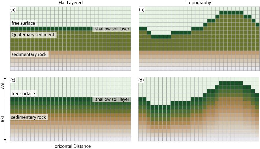
Alttext 4: Adding topography to a flat-layered model requires the addition or subtraction
of material, which is handled differently depending on local geology. — Figure 4.
Examples illustrating the recommendations for accommodating topography in the Cascadia seismic velocity model (CVM). Grid points above the free surface are above sea level (ASL) and points below the free surface are below sea level (BSL). A, B, At sites with Quaternary sediment, topography is accommodated by adding or removing material from the base of the Quaternary sediment layer, in order to preserve the shape of the Quaternary-Tertiary interface. C, D, For all other sites, topography is accommodated by adding or removing material from the deeper rock layers.

Additional Modifications

In addition to the updates detailed above, we also adjusted the V_P values at select locations in the model, in order to replace unrealistic V_P/V_S ratio values that were contained in model v1.6. These values typically occurred in localized regions around the edges of the Puget Lowland and Portland area basins, where independent studies informed V_P and V_S, and produced V_P/V_S ratios ~1. We set a minimum V_P/V_S ratio value of 1.45 throughout the model, which was attained by adjusting V_P values where necessary. This is the only modification we made that was applied at all depths of the CVM.

Simulation of the 2001 M6.8 Nisqually Earthquake

To quantify the effect of adding a shallow soft soil model to the Stephenson and others (2017) CVM, we ran numerical simulations of the M6.8 Nisqually, Washington, intraslab earthquake using the original (v1.6) and updated (v1.7) seismic velocity models. Simulations were run using the 3D seismic modeling code SW4 (Petersson and Sjögreen, 2022). We used the earthquake source model developed for the Nisqually earthquake by Frankel and others (2009), which consisted of two-point sources at 55 km depth. Seismic wave energy was resolved up to ~1.75 Hz using a minimum grid spacing of 20 m and V_Smin=150 m/s. (We note that for ground motion simulations, care should be taken with the extremely low V_S values at z=0 for select sites; in most cases, a minimum V_S cutoff should be applied.) We focused on simulating ground motions in the greater Seattle area, given its relatively high density of seismic stations during the Nisqually earthquake and variety of shallow soil types, ranging from artificial fill to outcrops of Tertiary sedimentary rock (Frankel and others, 2009). Recordings of the M6.8 Nisqually earthquake were downloaded from the EarthScope Consortium Web Services using the UW (Pacific Northwest Seismic Network; University of Washington, 1963) and GS (Albuquerque Seismological Laboratory [ASL], 1980) networks and processed using ObsPy (Beyreuther and others, 2010). Peak ground velocities and Fourier spectral amplitudes were computed using the geometric mean of the horizontal components.

Focusing on the greater Seattle area, we note that ground motion estimates using the updated CVM with a shallow soil velocity model are clearly more representative of the underlying geology compared to the original CVM (fig. 5). In addition, the misfit relative to the recorded data for the M6.8 Nisqually earthquake is reduced when using the shallow soil velocity model, particularly for low V_S30 sites (<250 m/s; fig. 6A). Because our soil velocity model layer is relatively thin, the most substantial effect is on shorter period seismic energy (≤2 s; fig. 6B). Comparisons of 1 s Fourier spectral energy using a CVM with and without a shallow soil velocity model clearly show that the most substantial changes are observed in the heavily industrialized Duwamish Waterway, which is composed of a northwest-southeast trending swath of artificial fill and alluvium with low V_S30 in central Seattle (fig. 7). Although there is a paucity of strong ground motion recordings in the Pacific Northwest for comparisons, we expect that modifying the CVM to better reflect the local shallow soil conditions and explicitly include regional V_S30 information will result in more accurate shaking estimates for future high-frequency ground motions (Stone and others, 2023; Grant and others, in press).

Alttext 5: Simulated estimates of peak ground velocity are different using the new
Cascadia seismic velocity model compared to the original. The new model reveals higher
peak ground velocity. — Figure 5.
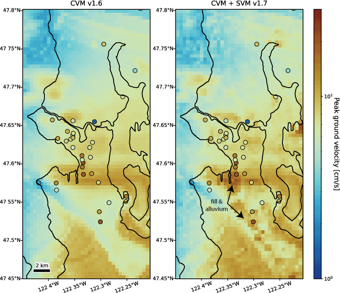
Maps of peak ground velocity from simulations of the 2001 magnitude 6.8 Nisqually, Washington, earthquake without (left) and with (right) a shallow soil velocity model in the greater Seattle area, Washington. Note the higher peak ground velocities (PGV) in the simulations with shallow soil information in regions with artificial fill and alluvium. Observed PGV at seismic stations throughout the Seattle region are shown as circles where the fill reflects values in the color bar. *Left*, model version 1.6 of the Cascadia seismic velocity model (CVM; Stephenson and others, 2017). *Right*, version 1.7 as presented in this report. cm/s, centimeters per second.

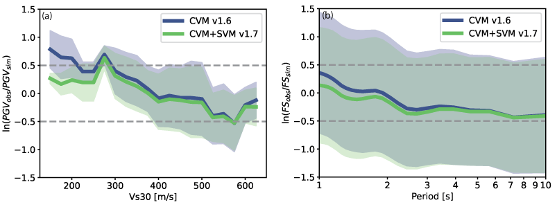
Alttext 6: Simulations using the new Cascadia seismic velocity model exhibit lower
bias at low Vs30 sites and at shorter periods compared to the original model. — Figure 6.
Plots of (A) bias and standard deviation in peak ground velocity (PGV, observed and simulated) misfits as a function of site time-averaged shear-wave velocity to a depth of 30 meters (m) (V_S30) (Geyin and Maurer, 2023), and (B) bias and standard deviation for Fourier spectra (FS) as a function of period for the 37 stations shown in figure 5. Positive bias indicates that the simulations underestimate the observed values, and negative bias indicates the simulations overestimate the observed values. Recordings with evidence of liquefaction have been removed. The blue line is model version (v) 1.6 of the Cascadia seismic velocity model (CVM; Stephenson and others, 2017). The green line is v1.7 that includes a shallow soil-velocity model (SVM) as presented in this report. s, second; m/s, meter per second; ln, natural logarithm.

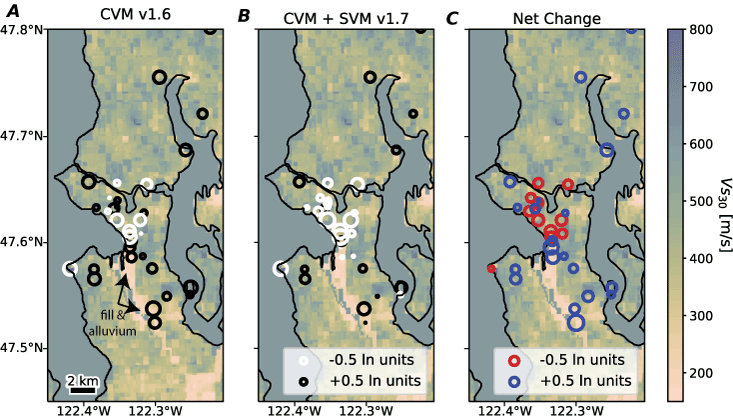
Alttext 7: Simulations using the new Cascadia seismic velocity model produce different
1.5 second Fourier spectral amplitudes compared to the original model. — Figure 7.
Maps of misfit in 1.5 hertz (Hz) Fourier spectral energy from simulations of the 2001 magnitude 6.8 Nisqually, Washington, earthquake without (A) and with (B) a shallow soil velocity model in the greater Seattle area, Washington. For context, time-averaged shear-wave velocity (V_S) to a depth of 30 meters (m) (V_S30) values from Geyin and Maurer (2023) are shown for both panels. A, B, The most substantial changes in misfit occur in the northwest-southeast trending strip of artificial fill and alluvium along the Duwamish Waterway (V_S ≤~200 m/s; pale pink color). Larger circles indicate higher misfits, with simulation overprediction shown in white and simulation underprediction shown in black. C, Net change between the misfits shown in parts A and B. Blue circles represent a lower misfit using the updated Cascadia seismic velocity model (CVM) plus shallow soil-velocity model (SVM) version (v) 1.7, and red circles represent a larger misfit using the updated model v1.7. Bigger circles indicate a larger change between parts A and B. CVM, v1.6 of the Cascadia seismic velocity model (Stephenson and others, 2017); SVM, shallow soil-velocity model as presented in this report (v1.7); ≤, less than or equal to; ~, approximately; m/s, meter per second.

Summary and Opportunities for Model Improvement

We updated the Stephenson and others (2017) 3D seismic velocity model for the Cascadia Subduction Zone region to include a shallow-soil velocity model with the option of adding user-specified topography. Visual comparisons of the original (v1.6) and updated (v1.7) CVM at various depths are shown in figure 8. Although these model updates reflect an advance in characterizing the shallow seismic velocities in the CVM, below we outline several areas where future improvements could be made.

Improving Regional V_S30 Models

Multiple V_S30 models are available for the Pacific Northwest, including the global V_S30 mosaic (Heath and others, 2020), a topographic slope-based map (Wald and Allen, 2007), and the machine-learning-based V_S30 map used here (Geyin and Maurer, 2023). In this study, the input V_S30 map had a substantial effect on the resulting soil velocity model, and therefore, the resulting ground motions in 3D earthquake simulations. We found that the topographic slope-based model did not reproduce ground motions from the M6.8 Nisqually earthquake as well as other V_S30 maps. The global mosaic map is more prevalent and is used for several applications, including for creating ShakeMaps from observed earthquakes and developing scenario ShakeMaps for hypothetical earthquakes (Wirth and others, 2020). However, because the global mosaic uses V_S30 maps developed by individual States in the Pacific Northwest, there are substantial contrasts in the V_S30 estimates across the Oregon-Washington border that are not reflective of actual changes in Earth structure. These artificial V_S30 contrasts skew the comparative hazard estimates across States in the western United States, and potentially affect risk mitigation and response planning. Therefore, for this study, we chose to use the Geyin and Maurer (2023) V_S30 map, which was developed using a consistent approach across Washington, Oregon, and California, and performed well at reproducing the observed ground shaking from the M6.8 Nisqually earthquake. However, the Geyin and Maurer (2023) V_S30 map does not extend into British Columbia, which is necessary to accurately characterize the full extent of the Cascadia Subduction Zone. This results in differences in our shallow soil velocity model across the United States (V_S30 from Geyin and Maurer, 2023) and Canada (V_S30 from the topographic-slope based work of Wald and Allen, 2007) border (fig. 8A, C, E, and G). Efforts to improve regional V_S30 maps could focus on applying a consistent approach across state and national borders to minimize artifacts, as well as including a wider geographic region that spans the full extent of the Cascadia Subduction Zone.

Constraining V_S at Intermediate Depths

The measured V_S profiles that were used to develop the shallow-soil model constrain seismic wave velocities at shallow depths. Typical measured V_S profiles extended to ≤50 m below the surface for rocks sites and up to a few hundred meters for some Puget Sound region sites (Grant and others, in press). Meanwhile, for the continental crust and mantle, V_S was typically constrained by ambient noise seismic tomography that is likely not sensitive to seismic velocities shallower than a few kilometers (Moschetti and others, 2007). This leaves a gap in independent constraints on V_S at depths between a few tens to hundreds of meters and a few kilometers, which made it challenging to make informed decisions about how to merge the shallow-soil velocity model with the seismic velocities in the Stephenson and others (2017) v1.6 model.

This problem is particularly acute for sites within our “other” category (typically rock sites), where we linearly interpolate between the seismic velocities determined by our generalized soil velocity profile at z=50 m to the Stephenson and others (2017) seismic velocities at z=100 m. The Stephenson and others (2017) V_S values at 100 m depths are ~2,500 m/s, which is quite fast compared to a “typical” rock site in the western United States (V_S ~1,400 m/s; Boore and Joyner, 1997). However, we note that most of the data used to develop the Boore and Joyner (1997) generic V_S profile for a rock site were from California. For comparison, Wong and others (2011) estimated V_S profiles for strong motion sites in western Washington using spectral analysis of surface wave velocities. Although most of the sites analyzed were located on Quaternary sediment, results at their sites GNW (intrusive rock) and 7027 (Tertiary sedimentary rock) reached a V_S of ~2,000 m/s at a depth of ~50 m. This suggests that a steep V_S gradient in the top ~50 m may be reasonable for Pacific Northwest rock sites. Further, we note that simulated ground motions would likely be underestimated if our intermediate-depth seismic velocities were too fast. On the contrary, our rock sites tend to slightly overestimate ground motions from the M6.8 Nisqually earthquake at sites outside of the Puget Lowland. Overall, constraining seismic velocities at these intermediate depths could help resolve this ambiguity and ensure more accurate estimates of ground motions in future Cascadia Subduction Zone region earthquake simulations.

Integrating New Onshore and Offshore Studies

Outside of the Puget Sound region, v1.6 and v1.7 of the CVM predominantly use V_S tomography results from Moschetti and others (2007) to define the seismic velocities in the continental crust and mantle beneath onshore locations. Offshore portions of the model were assigned properties based on numerous active source studies (Stephenson, 2007, and references therein), which were published between 1994–2002. The geometry of the subducting Juan de Fuca slab was derived from contours developed by McCrory and others (2012).

Since these studies were published, there have been numerous ongoing efforts to constrain the seismic velocity structure of the onshore and offshore Cascadia Subduction Zone region. Recent experiments include the Cascadia Initiative (Toomey and others, 2014), Ridge-to-Trench experiment (Han and others, 2016), CASIE21 (Carbotte and others, 2024; Canales and others, 2023), and Cascadia202X experiments (Tréhu and others, 2022), among many others (Tréhu and others, 2018, and references therein). New estimates to the top of the Juan de Fuca slab are also being continually refined (Hayes and others, 2018), and new high-resolution bathymetry (Dartnell and others, 2021) and constraints on offshore site effects (Gomberg, 2018) are being obtained. Coordinated efforts to incorporate the best available scientific results into the CVM, as well as detailed frameworks for model updates and validation, could contribute to the development of a true “community” seismic velocity model (Small and others, 2017).

Adding Faults and Damage Zones

Regional seismic velocity models may explicitly include impedance contrasts along mapped faults (for example, the San Francisco Bay area model by Aagaard and others, 2020; the Southern California CVM-H model by Shaw and others, 2015). At present, the Cascadia velocity model only includes the Seattle Fault, which bounds the southern edge of the Seattle basin. Faults often delineate geologic boundaries in the crust that can substantially influence wave propagation and give rise to effects like basin-edge surface waves. The addition of mapped Quaternary faults in the Pacific Northwest, both onshore and offshore, could strengthen the model results, although we acknowledge that many active faults are likely poorly constrained or yet unknown.

In addition, it may also be reasonable to include low-velocity fault damage zones in the vicinity of mapped faults. Observations have shown that mature fault systems often have an associated damage zone surrounding the fault down to a depth of several kilometers, which can reduce local seismic wave velocities up to 50 percent (Cochran and others, 2009; Graves and Pitarka, 2016). Including a fault damage zone can have multiple implications for earthquake ground motion simulations, including potentially acting as a waveguide and affecting shallow rupture propagation (Graves and Pitarka, 2016; Stone and others, 2023).

Expanding Geographic Boundaries

Currently, the CVM has a southernmost extent near Eureka, California (40.2° N.), an easternmost extent that terminates in the western foothills of the Cascade Range (−121.0° W.), and a northernmost extent slightly north of Vancouver, British Columbia (50.0° N.). To facilitate statewide hazard and risk assessments, as well as to model crustal fault earthquake scenarios east of the Cascade Range, the CVM would need to extend eastward to capture all of Washington and Oregon States. Similarly, extending the northern edge of the CVM to the Queen Charlotte Fault would allow it to encapsulate the full extent of the Cascadia subduction system, including the subducting Explorer segment of the Juan de Fuca Plate. To the south, extending the model to south-central California would allow numerical simulations to capture the feasible range of felt shaking during a Cascadia Subduction Zone earthquake (Wirth and others, 2020) and possible long-period amplification of seismic wave energy in the sediments of the Central Valley in California. Numerous seismic velocity models exist in California (Small and others, 2017; Aagaard and Hirakawa, 2021) that could be stitched to the Cascadia velocity model to encapsulate the entire U.S. West Coast. However, we note that it is often challenging to merge seismic velocity models with different resolutions and spatial extents (Zhang and Ben-Zion, 2024).

Sedimentary Basins in the Willamette Valley and Puget Sound Area

The heavily populated region spanning from Eugene to Portland, Oregon, is characterized by sedimentary material in the Willamette Valley and Tualatin and Portland basins. Version 1.6 of the CVM contains a ~1-kilometer (km)-thick layer of Tertiary sedimentary rock in the Portland-Tualatin region. With the updates included in this release (v1.7), we are likely better characterizing the shallow Quaternary sediment layer in this region (and thus, short period energy greater than ~0.5 Hz), but the deeper kilometer-scale structure is still poorly constrained. Recent studies have improved our knowledge of the structure of the Tualatin and Portland basins, demonstrating that these basins reach depths of ~6 km and ~2 km, respectively, and may substantially affect earthquake ground shaking (McPhee and others, 2014; Frankel and Grant, 2021; Stone and others, 2021). Improvements to the seismic velocity structure of the larger scale Willamette Valley are also needed to accurately characterize regional ground motions (Shimony and Sahakian, 2021).

In the Puget Sound region, the model for the Seattle basin in the CVM has been extensively validated using observations from local earthquakes (Frankel and others, 2009; Wirth and others, 2018a; Thompson and others, 2020, among others). Conversely, the Tacoma, Everett, Bellingham, and Georgia basins are characterized in the CVM, but have not been nearly as well-studied. Ground motion estimates from simulated earthquakes could be compared to data recorded in these basins, and details of their fine-scale structure (for example, basin depth, internal layering, and basin edge impedance contrasts) could be refined. In addition, existing studies with improved characterizations of the basin structure could be incorporated into the CVM (Molnar, 2011).

Overall, users should be aware of the limitations of the CVM, especially for areas where validation efforts using recordings of local earthquakes have been limited. However, we note that for non-basin sites, ground motion simulations performed using the CVM appear to match empirically derived ground motion models from global earthquakes (Frankel and others, 2018). Although moderate magnitude seismicity in the region is sparse, future validation efforts could attempt to exploit the limited number of M3–4+ earthquakes that occur throughout the Pacific Northwest each year, which are increasingly well-recorded due to the growing number of seismic stations in the region.

Conclusions

The three-dimensional (3D) seismic velocity model for the Cascadia Subduction Zone region has been an indispensable product in estimating ground motions and seismic hazard analyses throughout the Pacific Northwest (Stephenson, 2007; Stephenson and others, 2017). It has been used to inform key input parameters for empirical ground motion models (Ahdi and others, 2022) and as the backbone of 3D wave propagation simulations. The CVM has enabled the production of earthquake ground motion simulations in the Pacific Northwest—including hypothetical Cascadia Subduction Zone (Frankel and others, 2018; Wirth and others, 2018b) and crustal fault (Stone and others, 2022; 2023) earthquakes—which is essential to hazard mitigation and earthquake response planning in the seismically quiescent Cascadia Subduction Zone region. The results of these studies have been incorporated into the USGS National Seismic Hazard Model (Petersen and others, 2024) and have led to the strengthening of design requirements for tall buildings in the City of Seattle (Wirth and others, 2018a). As high-performance computing becomes increasingly powerful and 3D earthquake simulations are pushed to higher frequencies (Rodgers and others, 2020), regional seismic velocity models can be further developed to incorporate shallow soil information to produce accurate high frequency ground motions. This update to the Cascadia seismic velocity model (v1.7) combines a shallow soil velocity model (Grant and others, in press) with v1.6 of the CVM, which will allow for more accurate waveform modeling of short-period energy for scenario earthquakes in the Pacific Northwest. In addition, the option of adding user-specific topography, can enhance the ability of earthquake modelers to incorporate important 3D effects (Stone and others, 2022, 2023) that will affect the seismic wavefield.

Alttext 8: Comparisons demonstrate that the addition of a new soil velocity model
lowers shear wave velocities and reflects regional geology. — Figure 8.
Maps of depth slices through the updated Cascadia seismic velocity model (CVM) with a soil velocity model (version [v] 1.7, left panels) and the original v1.6 CVM (right panels). Note that v1.6 of the CVM, which only provided data in 100-meter (m) depth increments, was linearly interpolated between 0–100 m for inland sites to facilitate this comparison. Model v1.6 of the CVM from Stephenson and others (2017). Version 1.7 as presented in this report. m/s, meter per second; km, kilometer.

Figure 8.
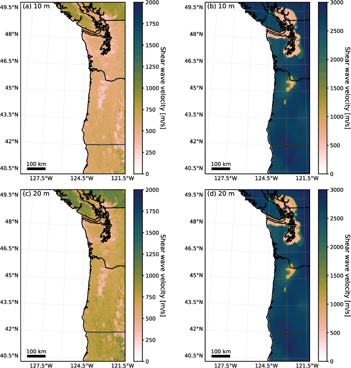
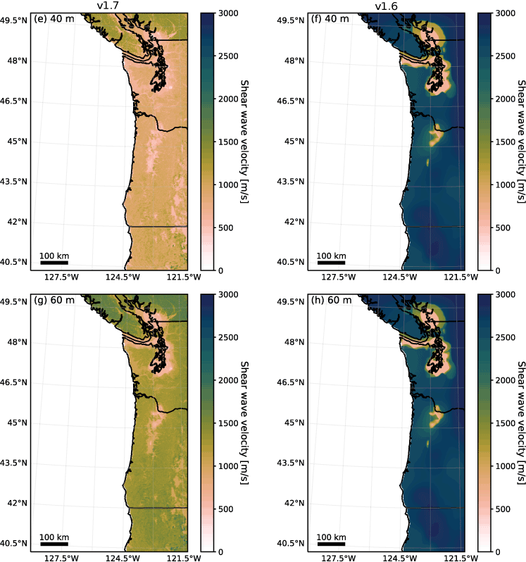
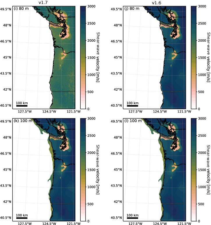
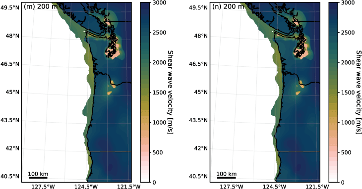
Maps of depth slices through the updated Cascadia seismic velocity model (CVM) with a soil velocity model (version [v] 1.7, left panels) and the original v1.6 CVM (right panels). Note that v1.6 of the CVM, which only provided data in 100-meter (m) depth increments, was linearly interpolated between 0–100 m for inland sites to facilitate this comparison. Model v1.6 of the CVM from Stephenson and others (2017). Version 1.7 as presented in this report. m/s, meter per second; km, kilometer.

References Cited

Aagaard, B.T., Graymer, R.W., Thurber, C.H., Rodgers, A.J., Taira, T., Catchings, R.D., Goulet, C.A., and Plesch, A., 2020, Science plan for improving three-dimensional seismic velocity models in the San Fransisco Bay region, 2019–24: U.S. Geological Survey Open-File Report 2020–1019, 37 p., https://doi.org/10.3133/ofr20201019.

Aagaard, B.T., and Hirakawa, E.T., 2021, San Francisco Bay region 3D seismic velocity model v21.1: U.S. Geological Survey data release, accessed August 2024, at https://doi.org/10.5066/P9TRDCHE.

Ahdi, S.K., Kwak, D.Y., Ancheta, T.D., Contreras, V., Kishida, T., Kwok, A.O., Mazzoni, S., Ruz, F., and Stewart, J.P., 2022, Site parameters applied in NGA-Sub database: Earthquake Spectra, v. 38, no. 1, p. 494–520, https://doi.org/10.1177/87552930211043536.

Ahdi, S.K., Stewart, J.P., Ancheta, T.D., Kwak, D.Y., and Mitra, D., 2017, Development of V_S profile database and proxy-based models for V_S30 prediction in the Pacific Northwest region of North America: Bulletin of the Seismological Society of America, v. 107, no. 4, p. 1781–1801, https://doi.org/10.1785/0120160335.

Albuquerque Seismological Laboratory [ASL], 1980, U.S. Geological Survey Networks [dataset]: International Federation of Digital Seismograph Networks, https://doi.org/10.7914/SN/GS.

Beyreuther, M., Barsch, R., Krischer, L., Megies, T., Behr, Y., and Wassermann, J., 2010, ObsPy—A Python toolbox for seismology: Seismological Research Letters, v. 81, no. 3, p. 530–533, https://doi.org/10.1785/gssrl.81.3.530.

Boore, D.M., and Joyner, W.B., 1997, Site amplifications for generic rock sites: Bulletin of the Seismological Society of America, v. 87, no. 2, p. 327–341, https://doi.org/10.1785/BSSA0870020327.

Burns, W.J., and Coe, D.E., 2012, Missoula Floods—Inundation extent and primary flood features in the Portland metropolitan area, Clark, Cowlitz, and Skamania Counties, Washington, and Clackamas, Columbia, Marion, Multnomah, Washington, and Yamhill Counties, Oregon: Oregon Department of Geology and Mineral Industries Interpretative Map Series 36, scale 1:8,200, accessed August 1, 2024, at https://pubs.oregon.gov/dogami/ims/p-ims-036.htm.

Canales, J.P., Miller, N.C., Baldwin, W., Carbotte, S.M., Han, S., Boston, B., Jian, H., Collins, J., and Lizarralde, D., 2023, CASIE21‐OBS—An open‐access, OBS controlled‐source seismic data set for investigating the structure and properties of the Cascadia accretionary wedge and the downgoing Explorer–Juan de Fuca–Gorda Plate System: Seismological Research Letters, v. 94, no. 4, p. 2093–2109, https://doi.org/10.1785/0220230010.

Carbotte, S.M., Boston, B., Han, S., Shuck, B., Beeson, J., Canales, J.P., Tobin, H., Miller, N., Nedimovic, M., Trehu, A., Lee, M., Lucas, M., Jian, H., Jiang, D., Moser, L., Anderson, C., Judd, D., Fernandez, J., Campbell, C., Goswami, A., and Gahlawat, R., 2024, Subducting plate structure and megathrust morphology from deep seismic imaging linked to earthquake rupture segmentation at Cascadia: Science Advances, v. 10, no. 23, https://doi.org/10.1126/sciadv.adl3198.

Cochran, E.S., Li, Y.-G., Shearer, P.M., Barbot, S., Fialko, Y., and Vidale, J.E., 2009, Seismic and geodetic evidence for extensive, long-lived fault damage zones: Geology, v. 37, no. 4, p. 315–318, https://doi.org/10.1130/G25306A.1.

Cui, Y., Miller, D., Schiarizza, P., and Diakow, L.J., 2017, British Columbia digital geology (data ver. 2019–12–19): British Columbia Ministry of Energy, Mines and Petroleum Resources, British Columbia Geological Survey Open File 2017–8, 9 p., database accessed August 1, 2024, at https://www2.gov.bc.ca/gov/content/industry/mineral-exploration-mining/british-columbia-geological-survey/geology/bcdigitalgeology.

Dartnell, P., Conrad, J.E., Watt, J.T., and Hill, J.C., 2021, Composite multibeam bathymetry surface and data sources of the southern Cascadia margin offshore Oregon and northern California: U.S. Geological Survey data release, https://doi.org/10.5066/P9C5DBMR.

Eberhart-Phillips, D., Reyners, M., Bannister, S., Chadwick, M., and Ellis, S., 2010, Establishing a versatile 3-D seismic velocity model for New Zealand: Seismological Research Letters, v. 81, no. 6, p. 992–1000, https://doi.org/10.1785/gssrl.81.6.992.

Fichtner, A., Trampert, J., Cupillard, P., Saygin, E., Taymaz, T., Capdeville, Y., and Villaseñor, A., 2013, Multiscale full waveform inversion: Geophysical Journal International, v. 194, no. 1, p. 534–556, https://doi.org/10.1093/gji/ggt118.

Frankel, A.D., Carver, D.L., and Williams, R.A., 2002, Nonlinear and linear site response and basin effects in Seattle for the M6.8 Nisqually, Washington, earthquake: Bulletin of the Seismological Society of America, v. 92, no. 6, p. 2090–2109, https://doi.org/10.1785/0120010254.

Frankel, A., and Grant, A., 2021, Site response, basin amplification, and earthquake stress drops in the Portland, Oregon area: Bulletin of the Seismological Society of America, v. 111, no. 2, p. 671–685, https://doi.org/10.1785/0120200269.

Frankel, A.D., and Stephenson, W.J., 2000, Modeling observed ground motions in Seattle using three-dimensional simulations: Bulletin of the Seismological Society of America, v. 90, no. 5, p. 1251–1267. https://doi.org/10.1785/0119990159

Frankel, A., Stephenson, W., and Carver, D., 2009, Sedimentary basin effects in Seattle, Washington—Ground-motion observations and 3D simulations: Bulletin of the Seismological Society of America, v. 99, no. 3, p. 1579–1611, https://doi.org/10.1785/0120080203.

Frankel, A.D., Stephenson, W.J., Carver, D.L., Williams, R.A., Odum, J.K., and Rhea, S., 2007, Seismic hazard maps for Seattle, Washington incorporating 3D sedimentary basin effects, nonlinear site response, and rupture directivity: U.S. Geological Survey Open-File Report 2007–1175, 77 p. https://doi.org/10.3133/ofr20071175

Frankel, A., Wirth, E., Marafi, N., Vidale, J., and Stephenson, W., 2018, Broadband synthetic seismograms for magnitude 9 earthquakes on the Cascadia megathrust based on 3D simulations and stochastic synthetics, Part 1—Methodology and overall results: Bulletin of the Seismological Society of America, v. 108, no. 5A, p. 2347–2369, https://doi.org/10.1785/0120180034.

Friedman Alvarez, C.D., Stephenson, W.J., Leeds, A.L., and Lindberg, N.S., 2024, Miscellaneous microtremor array datasets from the Puget Lowland, Washington State: U.S. Geological Survey data release, accessed August 1, 2024, at https://doi.org/10.5066/P9M5344V.

Geyin, M., and Maurer, B.W., 2023, U.S. national V_S30 models and maps informed by remote sensing and machine learning: Seismological Research Letters, v. 94, no. 3, p. 1467–1477, https://doi.org/10.1785/0220220181.

Gomberg, J., 2018, Cascadia onshore-offshore site response, submarine sediment mobilization, and earthquake recurrence: Journal of Geophysical Research Solid Earth, v. 123, no. 2, p. 1381–1404, https://doi.org/10.1002/2017JB014985.

Grant, A.R.R., Wirth, E.A., and Stone, I., in press, A soil velocity model for improved ground motion simulations in the U.S. Pacific Northwest: Seismica.

Graves, R.W., and Aagaard, B.T., 2011, Testing long-period ground-motion simulations of scenario earthquakes using the M_w 7.2 El Mayor–Cucapah mainshock—Evaluation of finite-fault rupture characterization and 3D seismic velocity models: Bulletin of the Seismological Society of America, v. 101, no. 2, p. 895–907, https://doi.org/10.1785/0120100233.

Graves, R., and Pitarka, A., 2016, Kinematic ground‐motion simulations on rough faults including effects of 3D stochastic velocity perturbations: Bulletin of the Seismological Society of America, v. 106, no. 5, p. 2136–2153, https://doi.org/10.1785/0120160088.

Han, S., Carbotte, S.M., Canales, J.P., Nedimović, M.R., Carton, H., Gibson, J.C. and Horning, G.W., 2016, Seismic reflection imaging of the Juan de Fuca plate from ridge to trench—New constraints on the distribution of faulting and evolution of the crust prior to subduction: Journal of Geophysical Research Solid Earth, v. 121, no. 3, p. 1849–1872, https://doi.org/10.1002/2015JB012416.

Hartzell, S., Meremonte, M., Ramírez‐Guzmán, L., and McNamara, D., 2013, Ground motion in the presence of complex topography—Earthquake and ambient noise sources: Bulletin of the Seismological Society of America, v. 104, no. 1, p. 451–466, https://doi.org/10.1785/0120130088.

Hauksson, E., Yang, W., and Shearer, P.M., 2012, Waveform relocated earthquake catalog for southern California (1981 to June 2011): Bulletin of the Seismological Society of America, v. 102, no. 5, p. 2239–2244, https://doi.org/10.1785/0120120010.

Hayes, G.P., Moore, G.L., Portner, D.E., Hearne, M., Flamme, H., Furtney, M. and Smoczyk, G.M., 2018, Slab2, a comprehensive subduction zone geometry model: Science, v. 362, no. 6410, p. 58–61, https://doi.org/10.1126/science.aat4723.

Heath, D.C., Wald, D.J., Worden, C.B., Thompson, E.M., and Smoczyk, G.M., 2020, A global hybrid V_S30 map with a topographic slope-based default and regional map insets: Earthquake Spectra, v. 36, no. 3, p. 1570–1584, https://doi.org/10.1177/8755293020911137.

Johnson, S.Y., Dadisman, S.V., Childs, J.R., and Stanley, W.D., 1999, Active tectonics of the Seattle fault and central Puget Sound, Washington—Implications for earthquake hazards: Geological Society of America Bulletin, v. 111, no.7, p. 1042–1053, https://doi.org/10.1130/0016-7606(1999)111<1042:ATOTSF>2.3.CO;2.

Jones, M.A., 1996, Thickness of unconsolidated deposits in the Puget Sound Lowland, Washington and British Columbia: U.S. Geological Survey Water-Resources Investigations Report 94–4133, 1 pl., scale 1:455,600, https://doi.org/10.3133/wri944133.

Lomax, A., Zollo, A., Capuano, P., and Virieux, J., 2001, Precise, absolute earthquake location under Somma–Vesuvius volcano using a new three-dimensional velocity model: Geophysical Journal International, v. 146, no. 2, p. 313–331, https://doi.org/10.1046/j.0956-540x.2001.01444.x.

Ludington, S., Moring, B.C., Miller, R.J., Flynn, K.S., and Hopkins, M.J., 2005, Preliminary integrated databases for the United States, Western States—California, Nevada, Arizona, and Washington (ver. 1.3, December 2007): U.S. Geological Survey Open-File Report 2005–1305, https://doi.org/ofr20051305.

Marafi, N.A., Grant, A., Maurer, B.W., Rateria, G., Eberhard, M.O., and Berman, J.W., 2021, A generic soil velocity model that accounts for near-surface conditions and deeper geologic structure: Soil Dynamics and Earthquake Engineering, v. 140, article 106461, https://doi.org/10.1016/j.soildyn.2020.106461.

McCrory, P.A., Blair, J.L., Waldhauser, F., and Oppenheimer, D.H., 2012, Juan de Fuca slab geometry and its relation to Wadati‐Benioff zone seismicity: Journal of Geophysical Research Solid Earth, v. 117, no. B9, https://doi.org/10.1029/2012JB009407.

McPhee, D.K., Langenheim, V.E., Wells, R.E., and Blakely, R.J., 2014, Tectonic evolution of the Tualatin basin, northwest Oregon, as revealed by inversion of gravity data: Geosphere, v. 10, no. 2, p. 264–275, https://doi.org/10.1130/GES00929.1.

Molnar, S., 2011, Predicting earthquake ground shaking due to one-dimensional soil layering and three-dimensional basin structure in SW British Columbia, Canada: Victoria, B.C., University of Victoria, Ph.D. dissertation, OCLC no. 1019487244, 160 p., https://library-archives.canada.ca/eng/services/services-libraries/theses/Pages/item.aspx?idNumber=1019487244.

Moschetti, M.P., Hartzell, S., Ramírez‐Guzmán, L., Frankel, A.D., Angster, S.J., and Stephenson, W.J., 2017, 3D ground‐motion simulations of M_w 7 earthquakes on the Salt Lake City segment of the Wasatch Fault Zone—Variability of long‐period ⁠(T≥1 s)⁠ ground motions and sensitivity to kinematic rupture parameters: Bulletin of the Seismological Society of America, v. 107, no. 4, p. 1704–1723, https://doi.org/10.1785/0120160307.

Moschetti, M.P., Ritzwoller, M.H., and Shapiro, N.M., 2007, Surface wave tomography of the western United States from ambient seismic noise—Rayleigh wave group velocity maps: Geochemistry, Geophysics, Geosystems, v. 8, no. 8, https://doi.org/10.1029/2007GC001655.

Mosher, D.C., and Johnson, S.Y., 2000, Juan de Fuca atlas – Neotectonics of the eastern Juan de Fuca Strait. A digital geological and geophysical atlas: Geological Survey of Canada Open-File no. 3931.

Nguyen, T.D., Bradley, B.A., Lee, R.L., and Graves, R.W., 2021, Full waveform tomography for the upper South Island region, New Zealand, in 2021 New Zealand Society for Earthquake Engineering (NZSEE) Annual Technical Conference, Christchurch, New Zealand, April 12–16, 2021, Proceedings: New Zealand Society for Earthquake Engineering Annual Technical Conference, accessed September 1, 2022, at https://repo.nzsee.org.nz/handle/nzsee/2429.

Petersen, M.D., Shumway, A.M., Powers, P.M., Field, E.H., Moschetti, M.P., Jaiswal, K.S., Milner, K.R., Rezaeian, S., Frankel, A.D., Llenos, A.L., Michael, A.J., Altekruse, J.M., Ahdi, S.K., Withers, K.B., Mueller, C.S., Zeng, Y., Chase, R.E., Salditch, L.M., Luco, N., Rukstales, K.S., Herrick, J.A., Girot, D.L., Aagaard, B.T., Bender, A.M., Blanpied, M.L., Briggs, R.W., Boyd, O.S., Clayton, B.S., DuRoss, C.B., Evans, E.L., Haeussler, P.J., Hatem, A.E., Haynie, K.L., Hearn, E.H., Johnson, K.M., Kortum, Z.A., Kwong, N.S., Makdisi, A.J., Mason, H.B., McNamara, D.E., McPhillips, D.F., Okubo, P.G., Page, M.T., Pollitz, F.F., Rubinstein, J.L., Shaw, B.E., Shen, Z.-K.S., Shiro, B.R., Smith, J.A., Stephenson, W.J., Thompson, E.M., Thompson Jobe, J.A., Wirth, E.A., and Witter, R.C., 2024, The 2023 U.S. 50-state national seismic hazard model—Overview and implications: Earthquake Spectra, v. 40, no. 1 https://doi.org/10.1177/87552930231215428.

Petersen, M.D., Shumway, A.M., Powers, P.M., Mueller, C.S., Moschetti, M.P., Frankel, A.D., Rezaeian, S., McNamara, D.E., Luco, N., Boyd, O.S., Rukstales, K.S., Jaiswal, K.S., Thompson, E.M., Hoover, S.M., Clayton, B.S., Field, E.H., and Zeng, Y., 2020, The 2018 update of the U.S. national seismic hazard model—Overview of model and implications, Earthquake Spectra, v. 36, no. 1, p. 5–41, https://doi.org/10.1177/8755293019878199.

Petersson, N.A., and Sjögreen, B., 2022, Geodynamics/SW4—SW4, version 3.0-beta2: Zenodo, Computational Infrastructure of Geodynamics web page, software release, accessed August 1, 2024, at https://zenodo.org/records/8322590.

Razafindrakoto, H.N.T., Bradley, B.A., and Graves, R.W., 2018, Broadband ground‐motion simulation of the 2011 M_w 6.2 Christchurch, New Zealand, earthquake: Bulletin of the Seismological Society of America, v. 108, no. 4, p. 2130–2147, https://doi.org/10.1785/0120170388.

Rodgers, A.J., Pitarka, A., Pankajakshan, R., Sjögreen, B., and Petersson, N.A., 2020, Regional‐scale 3D ground‐motion simulations of M_w 7 earthquakes on the Hayward Fault, northern California resolving frequencies 0–10 Hz and including site‐response corrections: Bulletin of the Seismological Society of America, v. 110, no. 6, p. 2862–2881, https://doi.org/10.1785/0120200147.

Roten, D., Olsen, K.B., and Takedatsu, R., 2019, Numerical simulation of M9 megathrust earthquakes in the Cascadia Subduction Zone: Pure and Applied Geophysics, v. 177, p. 2125–2141, https://doi.org/10.1007/s00024-018-2085-5.

Shaw, J.H., Plesch, A., Tape, C., Suess, M.P., Jordan, T.H., Ely, G., Hauksson, E., Tromp, J., Tanimoto, T., Graves, R., Olsen, K., Nicholson, C., Maechling, P.J., Rivero, C., Lovely, P., Brankman, C.M., and Munster, J., 2015, Unified structural representation of the southern California crust and upper mantle: Earth and Planetary Science Letters, v. 415, p. 1–15, https://doi.org/10.1016/j.epsl.2015.01.016.

Shimony, R., and Sahakian, V., 2021, Characterizing shallow structure and ground-motions in the Oregon Willamette Valley, with 3-D numerical modeling [abs.], in American Geophysical Union Fall Meeting, New Orleans, La., December 13–17, 2021, Abstracts: American Geophysical Union, no. T15D-0202, Bibcode 2021AGUFM.T15D0202S, accessed August 1, 2024, at https://ui.adsabs.harvard.edu/abs/2021AGUFM.T15D0202S/abstract.

Small, P., Gill, D., Maechling, P.J., Taborda, R., Callaghan, S., Jordan, T.H., Olsen, K.B., Ely, G.P., and Goulet, C., 2017, The SCEC unified community velocity model software framework: Seismological Research Letters, v. 88, no. 6, p.1539–1552, https://doi.org/10.1785/0220170082.

Stephenson, W.J., 2007, Velocity and density models incorporating the Cascadia subduction zone for 3D earthquake ground motion simulations, version 1.3: U.S. Geological Survey Open-File Report 2007–1348, 24 p., https://doi.org/10.3133/ofr20071348.

Stephenson, W.J., Reitman, N.G., and Angster, S.J., 2017, P- and S-wave velocity models incorporating the Cascadia subduction zone for 3D earthquake ground motion simulations, version 1.6—Update for Open-File Report 2007–1348 (ver. 1.1, Sept. 10, 2019): U.S. Geological Survey Open-File Report 2017–1152, 17 p., accessed August 29, 2024, at https://doi.org/10.3133/ofr20171152. [Supersedes USGS Open-File Report 2007–1348.]

Stone, I., Wirth, E.A. and Frankel, A.D., 2021, Structure and Q_P–Q_S relations in the Seattle and Tualatin Basins from converted seismic phases: Bulletin of the Seismological Society of America, v. 111, no. 3, p. 1221–1233, https://doi.org/10.1785/0120200390.

Stone, I., Wirth, E.A., and Frankel, A.D., 2022, Topographic response to simulated M_w 6.5–7.0 earthquakes on the Seattle Fault: Bulletin of the Seismological Society of America, v. 112, no. 3, p. 1436–1462, https://doi.org/10.1785/0120210269.

Stone, I., Wirth, E.A., Grant, A.R., and Frankel, A.D., 2023, 3-D wave propagation simulations of M_w 6.5+ earthquakes on the Tacoma Fault, Washington State, considering the effects of topography, a geotechnical gradient, and a fault damage zone: Bulletin of the Seismological Society of America, v. 113, no. 6, p. 2519–2542, https://doi.org/10.1785/0120230083.

Taborda, R., and Bielak, J., 2013, Ground‐motion simulation and validation of the 2008 Chino Hills, California, earthquake: Bulletin of the Seismological Society of America, v. 103, no. 1, p. 131–156, https://doi.org/10.1785/0120110325.

Thompson, M., Wirth, E.A., Frankel, A.D., Hartog, J.R., and Vidale, J.E., 2020, Basin amplification effects in the Puget Lowland, Washington, from strong‐motion recordings and 3D simulations: Bulletin of the Seismological Society of America, v. 110, no. 2, p. 534–555, https://doi.org/10.1785/0120190211.

Toomey, D.R., Allen, R.M., Barclay, A.H., Bell, S.W., Bromirski, P.D., Carlson, R.L., Chen, X., Collins, J.A., Dziak, R.P., Evers, B., Forsyth, D.W., Gerstoft, P., Hooft, E.E.E., Livelybrooks, D., Lodewyk, J.A., Luther, D.S., McGuire, J.J., Schwartz, S.Y., Tolstoy, M., Tréhu, A.M., Weirathmueller, M., and Wilcock, W.S.D., 2014, The Cascadia initiative—A sea change in seismological studies of subduction zones: Oceanography, special issue, v. 27, no. 2, p. 138–150, https://www.jstor.org/stable/24862164.

Tréhu, A., Carbotte, S., and Toomey, D., 2018, Towards a 3D model of the Cascadia Subduction Zone, in EarthScope Synthesis Workshop, Corvallis, Oregon, June 18–20, 2018, Summary Report: EarthScope, accessed August 1, 2024, at https://www.earthscope-program-2003-2018.org/research/synthesis_workshops/3D_model_of_Cascadia.html.

Tréhu, A., Hooft, E., Ward, K., Wirth, E., and Stone, I., 2022, Field report for the Cascadia2021 seismic node experiment: Corvallis, Oreg., Oregon State University, 34 p., accessed August 1, 2024, at https://blogs.oregonstate.edu/cascadia2021/2022/06/08/field-data-report/.

University of Washington, 1963, Pacific Northwest Seismic Network—University of Washington [dataset]: International Federation of Digital Seismograph Networks, https://doi.org/10.7914/SN/UW.

Wald, D.J., and Allen, T.I., 2007, Topographic slope as a proxy for seismic site conditions and amplification: Bulletin of the Seismological Society of America, v. 97, no. 5, p. 1379–1395, https://doi.org/10.1785/0120060267.

Wang, X., and Zhan, Z., 2020, Moving from 1-D to 3-D velocity model—Automated waveform-based earthquake moment tensor inversion in the Los Angeles region: Geophysical Journal International, v. 220, no. 1, p. 218–234, https://doi.org/10.1093/gji/ggz435.

Washington Geological Survey, 2021, Shear wave database—GIS data (ver. 1.3, previously released June, 2019): Washington Geological Survey Digital Data Series 17, database, accessed August 1, 2024, at https://fortress.wa.gov/dnr/geologydata/publications/data_download/ger_portal_shear_wave.zip.

West, L.T., Neilson, T., and Forson, C., 2019, Report on site class assessments for the Washington State school seismic safety project: Washington Geological Survey Open-File Report 2019–01, 214 p., accessed August 1, 2024, at http://www.dnr.wa.gov/publications/ger_ofr2019-01_school_seismic_site_class_report.pdf.

Wirth, E.A., Chang, S.W., and Frankel, A.D., 2018a, 2018 Report on incorporating sedimentary basin response into the design of tall buildings in Seattle, Washington: U.S. Geological Survey Open-File Report 2018–1149, 19 p., https://doi.org/10.3133/ofr20181149.

Wirth, E.A., Frankel, A.D., Marafi, N., Vidale, J E., and Stephenson, W.J., 2018b, Broadband synthetic seismograms for magnitude 9 earthquakes on the Cascadia megathrust based on 3D simulations and stochastic synthetics, Part 2—Rupture parameters and variability: Bulletin of the Seismological Society of America, v. 108, no. 5A, p. 2370–2388 https://doi.org/10.1785/0120180029.

Wirth, E.A., Grant, A., Marafi, N.A., and Frankel, A.D., 2020, Ensemble ShakeMaps for magnitude 9 earthquakes on the Cascadia Subduction Zone: Seismological Research Letters, v. 92, p. 199–211, https://doi.org/10.1785/0220200240.

Wirth, E.A., Grant, A.R., Stone, I.P., Stephenson, W.J., and Frankel, A.D., 2025, Data for ‘A 3-D Seismic Velocity Model for Cascadia with Shallow Soils & Topography, Version 1.7’: U.S. Geological Survey data release, https://doi.org/10.5066/P14HJ3IC.

Wirth, E.A., and Stone, I., 2024, CVM_topo (version 1.0): U.S. Geological Survey software release, accessed August 1, 2024, at https://doi.org/10.5066/P14RV2OV.

Wong, I.G., Stokoe, K.H., II, Cox, B.R., Lin, Y.-C., and Menq, F.-Y., 2011, Shear-wave velocity profiling of strong motion sites that recorded the 2001 Nisqually, Washington, earthquake: Earthquake Spectra, v. 27, no. 1, p. 183–212, https://doi.org/10.1193/1.3534936.

Zhang, H., and Ben-Zion, Y., 2024, Enhancing regional seismic velocity models with higher-resolution local results using sparse dictionary learning: Journal of Geophysical Research, v. 129, no. 1, https://doi.org/10.1029/2023JB027016.

Conversion Factors

U.S. customary units to International System of Units


Multiply	By	To obtain
Length
inch (in.)	2.54	centimeter (cm)
foot (ft)	0.3048	meter (m)
mile (mi)	1.609	kilometer (km)
Flow rate
inch per second (in./s)	2.54	centimeter per second (cm/s)
foot per second (ft/s)	0.3048	meter per second (m/s)

International System of Units to U.S. customary units


Multiply	By	To obtain
Length
centimeter (cm)	0.3937	inch (in.)
meter (m)	3.281	foot (ft)
kilometer (km)	0.6214	mile (mi)
Flow rate
centimeter per second (cm/s)	0.3937	inch per second (in./s)
meter per second (m/s)	3.281	foot per second (ft/s)

Abbreviations

>: greater than
<: less than
≤: less than or equal to
3D: three-dimensional
CVM: Cascadia seismic velocity model
M: earthquake magnitude
PGV: peak ground velocity
SVM: soil velocity model
V_P: P-wave or compressional wave velocity
V_S: S-wave or shear wave velocity
V_S30: time-averaged shear-wave velocity to a depth of 30 meters
V_S_min: minimum S-wave velocity
WA DNR: Washington Department of Natural Resources
USGS: U.S. Geological Survey

Disclaimers

Any use of trade, firm, or product names is for descriptive purposes only and does not imply endorsement by the U.S. Government.

Although this information product, for the most part, is in the public domain, it also may contain copyrighted materials as noted in the text. Permission to reproduce copyrighted items must be secured from the copyright owner.

Suggested Citation

Wirth, E.A., Grant, A.R., Stone, I.P., Stephenson, W.J., and Frankel, A.D., 2025, Three-dimensional seismic velocity model for the Cascadia Subduction Zone with shallow soils and topography, version 1.7: U.S. Geological Survey Open-File Report 2025–1045, 18 p., https://doi.org/10.3133/ofr20251045.

ISSN: 2331-1258 (online)

Study Area

Additional publication details
Publication type	Report
Publication Subtype	USGS Numbered Series
Title	Three-dimensional seismic velocity model for the Cascadia Subduction Zone with shallow soils and topography, version 1.7
Series title	Open-File Report
Series number	2025-1045
DOI	10.3133/ofr20251045
Publication Date	September 19, 2025
Year Published	2025
Language	English
Publisher	U.S. Geological Survey
Publisher location	Reston, VA
Contributing office(s)	Earthquake Science Center
Description	Report: vi, 18 p.; Data Release
Country	Canada, United States
State	British Columbia, California, Oregon, Washington
Other Geospatial	Cascadia Subduction Zone
Online Only (Y/N)	Y