

Methodology and Technical Input for the 2025 U.S. List of Critical Minerals—Assessing the Potential Effects of Mineral Commodity Supply Chain Disruptions on the U.S. Economy
Links
- Document: Report (3.17 MB pdf) , HTML , XML
- Data Release: USGS data release - U.S. Geological Survey Minerals Yearbook data for select mineral commodities referenced in “U.S. Geological Survey Methodology and Technical Input for the 2025 U.S. List of Critical Minerals—Assessing the Potential Effects of Mineral Commodity Supply Chain Disruptions on the U.S. Economy”
- Version History: Version History (3.01 KB txt)
- NGMDB Index Page: National Geologic Map Database Index Page (html)
- Download citation as: RIS | Dublin Core
Acknowledgments
The authors would like to thank Lee Bray, Chad Friedline, Robert Goodin, Ashley Hatfield, Daniel Hayba, Stephen Jasinski, Brian Jaskula, Natalie Juda, Kateryna Klochko, Graham Lederer, Timothy O’Brien, Emily Schnebele, Ruth Schulte, Robert R. Seal II, Miriam Stevens, and Colin Williams at the U.S. Geological Survey for their input and feedback. The authors would also like to thank the U.S. Bureau of Economic Analysis for providing detailed input-output tables for 2023, which were not publicly available at the time of publication, for use in this study.
Abstract
The Secretary of the Interior, acting through the Director of the U.S. Geological Survey, is tasked by section 7002 (“Mineral Security”) of title VII (“Critical Minerals”) of the Energy Act of 2020 (Public Law 116–260, December 27, 2020, 116th Congress) with reviewing and revising the methodology used to evaluate mineral commodity supply risk and the U.S. List of Critical Minerals (LCM) no less than every 3 years. Following two previous LCM assessments, this analysis represents the latest technical input for evaluating each mineral commodity’s supply risk and determining their recommended status on the LCM. We evaluated mineral commodity supply risk using two criteria: (1) an economic effects assessment that quantified the potential effects of various trade disruption scenarios on the U.S. economy, and (2) an examination of whether the mineral commodity’s U.S. supply chain relied on a sole domestic producer that represented a single point of failure. For the first criterion, postdisruption equilibrium quantities and prices for each mineral commodity were calculated based on their price elasticities of supply and demand and the availability of excess production capacity for each yearlong foreign trade disruption scenario. Subsequently, a nonlinear optimization routine was used with detailed economic input-output tables to estimate the potential economic effects on the U.S. economy of over 1,200 scenarios for 84 mineral commodities. After accounting for the probability of each scenario’s occurrence, the overall results are presented in terms of changes in U.S. gross domestic product (GDP) by individual industry and the economy overall. The results, which ranged from a net decrease in U.S. GDP of nearly $4.5 billion to a net increase of $33 million, largely reflect U.S. import dependency and world production concentration. Using the Jenks natural breaks optimization method, a statistical classification technique, we categorized the mineral commodities into several classes based on this overall risk quantification. Mineral commodities with annualized probability-weighted net decreases in U.S. GDP greater than $2 million were recommended for inclusion on the LCM. If a mineral commodity did not meet the threshold for inclusion on the LCM under the first criterion, its domestic supply chain was examined under the second criterion, which recommended a mineral commodity for inclusion on the LCM if there was only a single domestic producer. Ultimately, the two criteria resulted in the recommendation of the addition of six mineral commodities (in descending risk order, potash, silicon, copper, silver, rhenium, and lead) to and the removal of two mineral commodities (arsenic and tellurium) from the LCM. By using an economic effects assessment, the results of this analysis provide a prioritization that can also be compared directly against other risk analyses and the cost of various risk mitigation strategies.
Plain Language Summary
To quantify the risks associated with potential disruptions and to recommend mineral commodities for inclusion on the updated U.S. List of Critical Minerals, as required by the Energy Act of 2020, the U.S. Geological Survey developed an economic model to estimate the potential effects of foreign trade disruptions of mineral commodities on the U.S. economy. The results of the study recommend the addition of six mineral commodities (in descending risk order, potash, silicon, copper, silver, rhenium, and lead) to and the removal of two mineral commodities (arsenic and tellurium) from the List of Critical Minerals. The analysis also provides a prioritization based on the results. The economic model has several advantages over previous assessments including the ability to directly compare the results against other economic risks and the costs of initiatives aimed at reducing the risks.
Introduction
Reliable supplies of mineral commodities, which are used in a myriad of technologies—old and new—are necessary for maintaining and growing the U.S. economy. The concentration of mineral commodity production in a few countries and the high degree of reliance of the United States on imports from these countries increases the risks associated with foreign supply disruptions (Nassar and others, 2020). These risks have been exemplified in recent months as the Ministry of Commerce of the People’s Republic of China (MOFCOM) has placed controls and outright bans on the exports of several mineral commodities including antimony, gallium, and germanium to the United States (Ministry of Commerce of the People’s Republic of China, 2024).
The Secretary of the Interior, acting through the Director of the U.S. Geological Survey, is tasked by section 7002 (“Mineral Security”) of title VII (“Critical Minerals”) of the Energy Act of 2020 (Public Law 116–260, December 27, 2020, 116th Congress) with reviewing and revising the methodology used to evaluate mineral commodity supply risk and the U.S. List of Critical Minerals (LCM) no less than every 3 years. In fulfilling part of the requirements of the Energy Act of 2020, the U.S. Geological Survey (USGS) provides the technical input for identifying mineral commodities whose supply disruption poses the greatest risk to the U.S. economy and national security. The Energy Act of 2020 defines “critical minerals” as the minerals, elements, substances, or materials that “(i) are essential to the economic or national security of the United States; (ii) the supply chain of which is vulnerable to disruptions (including restrictions associated with foreign political risk, abrupt demand growth, military conflict, violent unrest, anti-competitive or protectionist behaviors, and other risks throughout the supply chain); and (iii) serve an essential function in the manufacturing of a product (including energy technology-, defense-, currency-, agriculture-, consumer electronics-, and healthcare-related applications), the absence of which would have significant consequences for the economic or national security of the United States” (Public Law 116–260, section 7002(c)(4)(A)). The Energy Act of 2020 followed Executive Order 13817, “A Federal Strategy To Ensure Secure and Reliable Supplies of Critical Minerals” (3 CFR, 2017 Comp, p. 397–399), which tasked the Secretary of the Interior with submitting to the Federal Register a draft list of minerals determined to be critical. The methodology used in the first List of Critical Minerals (LCM) in 2018 involved two quantitative criteria (the concentration of global mineral commodity production and U.S. net import reliance) and a qualitative examination of the importance of each mineral commodity’s use (Fortier and others, 2018). After the passage of the Energy Act of 2020, a new methodology that provided several enhancements to the original approach was used in determining the second LCM in 2022 (Nassar and Fortier, 2021). Using a risk modeling framework, the second assessment retained the U.S. net import reliance indicator and weighted the previous global production concentration indicator by measures of each producing country’s willingness and ability to continue to supply the United States. In addition, it converted the qualitative examination of each mineral commodity’s importance into a quantitative assessment using data on each mineral commodity consuming industry’s contributions to U.S. gross domestic product (GDP) and gross operating surplus. It also added a criterion for including any mineral commodity on the LCM if there was only a single domestic producer, which represented a potential single point of failure (SPOF) within the mineral commodity’s domestic supply chain.
The analysis presented in this report takes another major step forward in assessing the risk associated with foreign trade disruptions. While the analysis presented here retains the same conceptual framework as the previous assessments, it moves away from normalized indicators and toward an economic effects assessment. In this approach, the risks associated with foreign trade disruptions are assessed probabilistically, and the results are provided in terms of expected (or probability-weighted) net decreases in U.S. GDP at the level of individual industries and the economy overall. Our analysis, which was conducted using data for year 2023 (unless otherwise noted), assessed over 1,200 scenarios for 84 mineral commodities.
Methods
We used two criteria in recommending a mineral commodity for inclusion on the LCM. One criterion assessed the potential economic effects of foreign trade disruptions on the U.S. economy. The other criterion evaluated whether there was a single producer of that mineral commodity (for example, a sole mine or refinery) in the United States (referred to as a SPOF). The methodology used to estimate the potential economic effects was primarily based on Nassar and others (2024) and consists of three stages: scenario quantification, equilibrium displacement modeling, and economic impacts modeling. These three stages of the economic effects assessment are discussed in detail below. If a mineral commodity did not meet the first criterion, its domestic supply chain was reviewed using the information presented in the USGS Mineral Commodity Summaries (U.S. Geological Survey, 2025a) to determine if there was a SPOF within its domestic supply chain. Details regarding specific sources and methods are found in the appendixes, which were initially published as a preprint (Nassar and others, 2025) before being edited and formatted for release in this version of this publication.
Stages of the Economic Effects Assessment
Scenario Quantification
The first stage of the economic effects assessment defined a specific set of scenarios. These scenarios were ones in which U.S. net imports (imports minus exports) for the mineral commodity of concern from each trading partner country were completely restricted for an entire year. A scenario was thus developed for each mineral commodity–restricting country pair if that country was also a producer of the mineral commodity. Any positive U.S. net imports for that mineral commodity (when summed across all forms included in the analysis) from non-producing countries were allocated to producing countries proportionally to their share of world production. This step was added to account for the fact that positive net imports from non-producing countries must have, at some point, originated from producing countries.
For each mineral commodity, annualized country-level global production and trade data were collected by production stage (for example, mining) or mineral-commodity form (for example, ores and concentrates). Data availability allowed for the assessment of 84 mineral commodities. Of these 84, 31 represent different stages or forms of 11 mineral commodity supply chains: aluminum (alumina, aluminum, and bauxite), chromium (chemicals, chromite, ferroalloys, and metal), cobalt (chemicals and metal), copper (mined and refined), graphite (natural and synthetic), fluorspar (acidspar and metspar), manganese (alloys, dioxide, high-purity sulfate, metal, ore), nickel (mined and primary refined), silicon (ferroalloys and metal), titanium (ferroalloys, metal, mineral concentrates, pigment, and sponge), and zinc (mined and smelted). Magnesium compounds and magnesium metal were treated as separate mineral commodity supply chains given their distinct sources and uses. Mineral production data included primary production and, if applicable and available, secondary (specifically, end-of-life or post-consumer recycling) production by country. Production data were mainly obtained from the most recent USGS publications, although other sources were used where necessary (refer to appendix 1 for details). For a few mineral commodities, secondary production data were only available by region or for the entire world. In cases where it was not possible to allocate these secondary production data to individual countries, the reported regional production quantities were treated as if they were a single entity in the scenario.
Global trade data were obtained from the Global Trade Tracker database (Zen Innovations AG, 2025) using the Harmonized Tariff Schedule of the United States (HTS) and Schedule B codes identified in appendix 2 for the imports and exports of each mineral commodity, respectively. The trade data were obtained from the U.S. perspective (meaning as reported by the United States) unless the trade data from the trade partner country’s perspective were determined to be more representative for the mineral commodity (refer to appendix 2 for details). Production and trade data were converted into elemental content (for example, the antimony content of antimony trioxide) to allow for summation across different chemical forms and were calculated net of any reimports or reexports (meaning that trade flows were calculated exclusive of the flows of commodities that were previously recorded as exports or imports, respectively, in substantiality the same condition) (International Trade Administration, 2015). Trade codes were selected to reflect the chemical forms (typically alloys, compounds, concentrates, metals, ore, and scrap) that were produced by the associated production processes up to the supply chain process associated with the identified consuming industries (as explained in the “Economic Impacts Modeling” section of this report). Additional notes and assumptions are provided in appendixes 1 and 2 for production and trade data, respectively.
Equilibrium Displacement Modeling
In the second stage of the economic effects assessment, the production and trade data were allocated to two regions or markets—the restricting country and the rest of the world—that varied by scenario. The quantity that was disrupted (∆Q) in each scenario (s) for each mineral commodity (c) was set equal to the U.S. net imports from the restricting country (NI) for the year. A postdisruption equilibrium price (P′) and quantity (Q′) for the rest of the world were determined based on (1) the quantity disrupted, (2) excess production capacity of the mineral commodity in the rest of the world (κROW), (3) the mineral commodity’s price elasticities of supply (εS) and demand (εD), and (4) the predisruption quantity of the mineral commodity available (Q). Specifically, the postdisruption equilibrium price relative to the predisruption price (P) was determined as follows:
where n was the relative shift in quantity available (). The predisruption quantity of the mineral commodity available (Q) was defined as the sum of the predisruption quantity that was produced by the rest of the world (ψROW) and the net imports from the restricting country (NI):This approach defined the system boundaries of the mineral commodity market that would be available to the United States, which varied by scenario because the definition (and, in turn, the net imports and production) of the rest of the world varied depending on which country was the restricting country. A scenario in which the restricting country was the sole producer of the mineral commodity would yield a relative shift in quantity available (n) of 100 percent. (Note that no such scenario was encountered in this analysis.) Establishing the system boundaries in this manner implicitly assumes that the mineral commodity produced by the non-restricting countries would be available and thus could be diverted to the United States. It also assumes that the restricting country applies its export restrictions extraterritorially, meaning that its exports to countries other than the United States are prohibited from being reexported to the United States. This assumption would also apply to downstream materials (for example, rare earth permanent magnets) that were included in the trade data, thereby effectively prohibiting non-restricting countries from exporting materials that they processed if the precursor materials were originally sourced from the restricting country.
Postdisruption equilibrium prices were determined numerically by setting equation 1 equal to equation 2. With the postdisruption equilibrium price, the relative change in the postdisruption equilibrium quantity, also referred to as the net disruption level (n′), was determined as follows:
If the specified scenario resulted in a supply disruption greater than the available excess capacity in the rest of the world (κROW), then equation 3 simplified to:This simplification was possible because the supply curve was assumed to become vertical at the point in which all excess capacity was used—a reflection of the inability to increase supplies in the short-term beyond the estimated capacities. Under such scenarios, the demand curve intercepts the vertical portion of the supply curve thereby allowing the postdisruption equilibrium price to be calculated directly:
The growth in the production of the rest of the world () that was necessary to achieve the postdisruption equilibrium quantity was calculated as follows:
The derivations of these equations are provided by Nassar and others (2024).Following Shojaeddini and others (2025), each mineral commodity’s price elasticities of supply and demand were estimated using fixed effects models for panel data and two-stage dynamic ordinary least-squares along with autoregressive distributed lag models for time-series data (refer to appendix 3 for a summary of the elasticities used in the analysis). Where possible, short-run (1-year) price elasticities were used, and price elasticities of demand were estimated to include inventory releases as a demand category.
Data on production capacity by country were obtained from published sources (refer to appendix 1) or, if not available, were estimated for each producing country based on historical production. Specifically, for the latter, production capacity for each currently producing country was assumed to equal its maximum production that was reported during the preceding 5-year period (2019–2023) divided by 80 percent to simulate an assumed capacity utilization rate. Additionally, a linear ramp-up time of 6 months was assumed to be required to reach the reported or estimated production capacity by country.
Economic Impacts Modeling
Three intermediate results for each scenario were obtained from the equilibrium displacement modeling (stage 2 of the economic effects assessment): the postdisruption equilibrium price, quantity, and the growth in production for the rest of the world. In the third stage of the economic effects assessment—the economic impacts modeling—these results were used with detailed economic input-output (IO) tables for the United States in a nonlinear optimization routine to estimate the potential effects of the scenarios on the U.S. economy (specifically, net decreases in U.S. GDP by industry). The intuition behind the model is that, in the event of a supply disruption, economic actors (be they final consumers, industries, or governments) will attempt to reestablish their economic activity patterns as closely as possible to their predisruption levels (Oosterhaven and Bouwmeester, 2016). As described by Nassar and others (2024), the objective function of the optimization model therefore attempted to minimize the change between the predisruption and postdisruption interindustry intermediate demand, final demand, and value added across all industries, as follows:
wherez and z′
were the predisruption and postdisruption interindustry intermediate demand, respectively;
y and y′
were the predisruption and postdisruption final demand, respectively;
v and v′
were the predisruption and postdisruption value added, respectively; and
i, j
were subscripts that indicate individual industries.
The decision variables in the model were each industry’s postdisruption output (x′). Each industry’s final postdisruption final demand (y′) was determined using the Leontief equation (Leontief, 1951), which provided the overall supply and demand equilibrium for the U.S. economy:
where I was the identity matrix and A was the industry-by-industry direct requirements matrix. Additionally, values for individual postdisruption interindustry intermediate demand (z′) were calculated using the direct requirements matrix:Data for each of the predisruption parameters of equations 7, 8, and 9 (all reported in current [2023] U.S. dollars) were available for the United States from the U.S. Bureau of Economic Analysis (BEA) at the detailed 402-industry level for years 2007, 2012, and 2017 (U.S. Bureau of Economic Analysis, 2025). The BEA industry groupings generally correspond to the definitions of the North American Industry Classification System (NAICS), which was developed under the auspices of the Office of Management and Budget to coordinate and publish industry data by Federal statistical agencies (U.S. Census Bureau, 2024). At the detailed level, an industry consists of establishments that are primarily engaged in similar processes to produce a narrowly defined category of products or services (for example, the “Computer storage device manufacturing” industry with NAICS code 334112). Multiple industries make up a subsector (for example, the “Computer and electronic product manufacturing [334]” subsector), which itself falls within a specific sector (for example, the “Manufacturing [31–33]” sector) of the economy (Office of Management and Budget, 2022). The BEA publishes updates to the IO tables annually but only at aggregated levels (U.S. Bureau of Economic Analysis, 2025). These aggregated data are based on estimated detailed IO tables, which were provided to the authors (U.S. Bureau of Economic Analysis, written comm., October 31, 2024). The most recent data provided (for year 2023) were used in this analysis.
The optimization routine was subjected to several constraints, including a mineral commodity availability constraint:
This constraint specified that the total quantity of the mineral commodity used by industries in the United States—calculated as the product of each consuming industry’s output and its mineral consumption ratio (m), summed across all industries—must equal the total postdisruption quantity of the mineral commodity (M′) that was available under the specified disruption scenario. The quantity of the mineral commodity that was available after the supply disruption was based on the predisruption quantity consumed in the United States (M) and the net disruption level (n′) that was derived in equilibrium displacement modeling:
The implicit assumption here is that the quantity that would be available for consumption in the United States decreases in the same relative proportion as that of the rest of the world (outside of the restricting country).
For each mineral commodity, the predisruption quantity that was consumed in the United States was calculated as the sum of domestic primary and secondary production, net imports, and changes in inventories. Data for each of these were obtained from the same sources as those listed in appendixes 1 and 2, with additional data for inventories obtained from the latest USGS Mineral Commodity Summaries (U.S. Geological Survey, 2025a) where applicable. The calculated or “apparent” consumption quantity was split into specific applications that were linked to individual industries. For example, the use of barite to increase the density of drilling mud in the petroleum industry was connected to the “Drilling oil and gas wells [213111]” BEA industry. As much as possible, we aligned the trade codes used in the equilibrium displacement model to the forms of the mineral commodities that would be purchased by (or the supply chain processes that directly precede) the selected BEA consuming industries. In certain cases, connections were made further downstream if the direct consuming industries were determined to be too broad to reasonably capture the use of the mineral commodity in the application. For example, cobalt metal’s use in high-performance “superalloys” was connected downstream to the “Aircraft engine and engine parts manufacturing [336412]” and the “Turbine and turbine generator set units manufacturing [333611]” industries rather than the “Iron and steel mills and ferroalloy manufacturing [331110]” industry. Details regarding the application fractions and the BEA industry connections are provided in appendix 4.
The monetary value of the trade of the mineral commodity was added to the value of domestic production and inventory releases to provide an estimate for the value of the apparent consumption. The monetary value of domestic production and inventory releases was calculated as the product of the quantities produced and released and the price noted in appendix 3 for each mineral commodity. In turn, an apparent consumption unit value was calculated as the ratio of the monetary value to the quantity of the calculated apparent consumption.
Even at the detailed 402‑industry level, not all the output of each identified BEA industry uses the mineral commodity in question. For example, not all of the output of the “Drilling oil and gas wells [213111]” industry uses barite, and not all of the output of the “Semiconductor and related device manufacturing [334413]” industry uses gallium or germanium. To address this issue, Nassar and others (2024) used modified mineral consumption ratios that account for the portion of each BEA industry’s output that used the mineral commodity in question. In this analysis, we instead performed a streamlined IO table expansion. Specifically, each consuming BEA industry was split into two industries: one that consumes the mineral commodity and the other that does not. Because IO table expansion requires extensive additional data regarding the newly formed industries’ inputs from and outputs to all other industries and final demand (data which were not readily available), simplifications were required. One simplification was that the newly formed industries had the same relative production recipe (in terms of monetary inputs per unit of output) as the original industry from which they were disaggregated. This meant that the columns of the direct requirements table for the two new industries were unchanged from the original. The other simplification was that the newly formed industries’ outputs to the other industries and to final demand were all split using the same proportion, which was based on the share of the original industry’s output that was estimated to have used the mineral commodity in question. These proportions, by industry and mineral commodity, were estimated mainly using data on the revenues generated from the sales of specific product(s) as defined by the North American Product Classification System (NAPCS) and reported in the 2017 Economic Census (U.S. Census Bureau, 2020) and the 2018–2021 Annual Survey of Manufactures (U.S. Census Bureau, 2022). Other sources and methods were used where the NAPCS data did not provide sufficient disaggregation for the mineral commodity. Details are provided in appendix 4. Note that the newly formed industries were remerged after running the optimization routine in order to report the results across a consistent set of 402 industries. With expanded IO tables, the mineral consumption ratio was calculated as the ratio of the quantity of the mineral commodity consumed by that industry relative to that industry’s output in U.S. dollars.
Another constraint used in the model was an industry production capacity constraint, which required each industry’s output to maintain a positive value that does not exceed that of its capacity (xc):
Each industry’s output capacity was calculated by dividing its predisruption output by its capacity utilization rate, u. Data regarding annual capacity utilization rates for industries within the manufacturing, mining, and electric and gas utilities sectors of the United States were obtained from the Board of Governors of the Federal Reserve System (2024). As explained by Nassar and others (2024), these data were available at the 3‑digit or 4‑digit NAICS subsector level or equivalent, whereas the BEA IO tables were reported at the 4-, 5-, or 6‑digit NAICS level equivalent. The capacity utilization data at the 3- and 4‑digit levels were thus applied to the most appropriate level or sublevel, accordingly. For the remaining industries outside of the manufacturing, mining, and electric and gas utilities sectors, the capacity utilization rate was set to 80 percent, which was approximately the average utilization rate across all sectors with capacity utilization data in 2023 (Board of Governors of the Federal Reserve System, 2024).
Each consuming industry’s postdisruption value added (its postdisruption contribution to U.S. GDP) was calculated as follows:
Changes to an industry’s value added were thus due to changes in both its output and its expenditure on the mineral commodity, with the latter being determined by changes in the mineral commodity’s price and the quantity consumed postdisruption. Although the changes in the mineral commodity’s price were determined in the equilibrium displacement model, changes in the quantity of the mineral commodity consumed were determined endogenously within the economic impacts model as it was a function of the consuming industry’s postdisruption output.
Because the demand curve for each mineral commodity was estimated using a single price elasticity, it was necessary to introduce a price maximum for mineral commodities with highly inelastic demand under scenarios in which the quantity restricted was large enough that all excess production capacity in the rest of the world was used (in other words, where a nearly vertical demand curve intersected the vertical portion of the supply curve). The price maximum (Pmax) was based on the maximum willingness to pay for each consuming industry, which was assumed to take place when an industry’s entire value added was reduced to zero owing to the price increase of the mineral commodity consumed. The price maximum for each industry was therefore determined by setting equation 13 to zero:
An overall price maximum for each mineral commodity was determined to be the largest of the calculated industry price maximums that achieved market clearing based on the mineral availability constraint. This price maximum was ultimately only necessary for four mineral commodity scenarios: trade disruption from China of lutetium, samarium, thulium, and ytterbium.
The postdisruption value added for producing industries was calculated in a similar manner to that of consuming industries except that the price effect increased rather than decreased the industry’s value added, and a mineral production ratio (r) was used instead of a mineral consumption ratio:
Like the mineral consumption ratio, the mineral production ratio was calculated as the ratio of the predisruption mineral production quantity of that industry to its output in U.S. dollars. As with mineral consuming BEA industries, each mineral producing BEA industry (identified in appendix 1) was split into two industries: one that was directly associated with the mineral commodity’s production and the other that represented the remainder of the BEA industry. The monetary value of the production of the mineral commodity as a percent of the industry’s output was the basis for splitting the mineral commodity producing BEA industries. Note that the predisruption price used for domestic production (noted in appendix 3), which was used for splitting the BEA producing industries and calculating the value added of producing industries in equation 15, was not necessarily the same as the predisruption consumption price used in splitting the consuming BEA industries and calculating the value added of consuming industries in equation 13. This price difference reflects the fact that the predisruption domestic consumption prices were based on the unit value of domestic apparent consumption, which accounted for the value and quantity of not only domestic production but also net imports. Differences in production and consumption prices were mainly a reflection of the differences in the commodity forms produced and consumed domestically. Although the predisruption consumption and production prices were different, they were both increased postdisruption at the same rate using the price ratio that was calculated in the equilibrium displacement model (or the calculated price maximum).
As with the mineral commodity availability constraint (eq. 10), a mineral commodity production constraint was included in the optimization routine to match the equilibrium displacement model results:
As illustrated in equation 16, domestic production (ψUS) of the mineral commodity was assumed to grow at the same rate as the production of the rest of the world but was limited by the maximum reported or estimated capacity of production in the United States, κUS. This constraint only applied to mineral commodities for which the United States was a producer. Note that because of this growth in domestic mineral commodity production, it was necessary in certain scenarios to remove the industry output capacity constraint (xci) for the producing industries.
The postdisruption value added for all other industries (meaning those that were neither direct consumers nor producers of the mineral commodity in question) were calculated without the price effect term of equations 13 and 15:
This approach assumed that direct consuming industries absorbed the entire price increase, with none of the price increase being passed on to downstream industries or final consumers. This assumption is not wholly realistic in all cases as many industries have the market power to pass through price increases, but it may be a reasonable assumption in the short term. These non-producing, non-direct consuming industries would thus be affected by the disruption indirectly through the IO tables and the objective function (eqs. 7–9), which seeks to minimize changes to not only each industry’s value added but also each interindustry intermediate and final demand.
Increases in prices of mineral commodities were accounted for only in the value added variable and not the other variables (industry output, final demand, or interindustry intermediate demand). This approach allowed the IO model to remain in price equilibrium for all other goods and services, while still accounting for the effect of mineral commodities’ price increases on U.S. GDP.
The overall economic effect, or net decrease in U.S. GDP, was calculated as the sum of the changes in value added across all industries for a single scenario:
Note that in equation 18, a net decrease in U.S. GDP is presented as a positive value.
Model Implementation
To solve the convex optimization problem at the core of the economic impacts model, we used the Clarabel solver (Goulart and Chen, 2024), an interior-point method designed for second-order cone and quadratic programming. Clarabel was written in the Rust programming language and integrated through Python via CVXPY (2025), allowing for both speed and ease of embedding in high-level modeling workflows. Unlike some legacy solvers, it offers better handling of problem scaling and numerical precision, which can be especially important for economic applications involving large IO models. For model implementation, we used Python version 3.11.8 (Python Software Foundation, 2024), along with CVXPY version 1.6.5. Additional details are provided in appendix 5.
For each scenario, results included the postdisruption values for each industry’s output, interindustry intermediate demand, final demand, and value added. As noted earlier, the results for the newly formed industries were remerged after running the optimization routine in order to report the results across a consistent set of 402 industries. Additionally, net decreases in U.S. GDP were grouped into one of the following economic effects components: consuming industries reducing their output, consuming industries paying higher prices, producing industries increasing their output, producing industries receiving higher prices, and all other industries reducing their output.
Scenario Probabilities
Because not all scenarios are equally likely to occur, we estimated a probability for the occurrence of each scenario. The probability of an export restriction was set to 100 percent for 17 scenarios that represent China’s trade disruptions of the mineral commodities (antimony, bismuth, dysprosium, gadolinium, gallium, germanium, natural graphite, synthetic graphite, indium, lutetium, magnesium metal, molybdenum, samarium, tellurium, terbium, tungsten, and yttrium) that China’s MOFCOM has (as of this writing) explicitly identified as being either restricted or completely banned from being exported to the United States (Ministry of Commerce of the People’s Republic of China, 2024, 2025a, b). For all other scenarios, the probability of a country implementing a trade restriction on a given mineral commodity was obtained using the method developed in Ryter and Nassar (2025). These probabilities were calculated using an ensemble of several machine learning classifiers, each of which produced a probability estimate for each mineral commodity–country scenario. Exogenous variables such as prior trade barrier implementation (specifically, trade prohibition, quota, or licensing requirements) and global export dominance or dependence were used to train each classifier and inform its probability estimates. The median of the probabilities for the mineral production process or trade codes that most closely aligned with those selected in this analysis were used. Probabilities were unavailable for a few mineral commodity–country pairs. These pairs represent a small number (17 out of 1,205 scenarios) of low economic impact (with net decreases in U.S. GDP averaging less than $2 million) scenarios. For completeness, these scenarios were assigned a probability equal to the mean probability of all scenarios assessed (4 percent).
With the probabilities (ρ) assigned to each scenario, the expected value or probability-weighted net decrease in U.S. GDP across all scenarios (E[∆GDP]) for each mineral commodity was determined, as follows:
Risk Categorization
A statistical approach was used to categorize the risk results. Specifically, the classification of the probability-weighted net decrease in U.S. GDP was conducted using the Jenks natural breaks optimization method (Jenks, 1967), which aims to minimize variance within classes while maximizing variance between classes. This method provides optimized cutoff points based on the specified number of classes, allowing for differentiation between various economic effects. To determine the appropriate number of classes and avoid overfitting, the elbow method suggested by Satopaa and others (2011) was employed. Additional details are provided in appendix 6.
Results and Discussion
With 84 mineral commodities, 402 industries, and over 1,200 scenarios, the results of the analysis, which include changes in equilibrium prices and quantities, as well as changes in each industry’s output, interindustry intermediate demand, final demand, and contributions to U.S. GDP are too numerous to display and discuss in full in this report. Instead, below is a sampling of results for a single example mineral commodity, palladium (fig. 1), followed by a summary of the main result variable (the probability-weighted net decrease in U.S. GDP, which is presented as a positive value) for all mineral commodities by trade disruption scenario (table 1 and fig. 2), industry (table 2), and economic effects component (table 3). Palladium was selected as the example to present because it was one of only a few mineral commodities examined for which more than one trade disruption scenario contributed notably to its overall probability-weighted net decrease in U.S. GDP.
Results for Palladium
In figure 1A, the estimated supply and demand curves for palladium are displayed for a scenario in which U.S. net imports of palladium from Russia (a leading world producer and import source for the United States) were completely restricted for an entire year. The results indicate that the price would increase by 24 percent and the quantity available postdisruption would decrease by approximately 5 percent (the net disruption level, n′). This does not account for speculative (often temporary) price fluctuations in the cash market, but rather reflects the change in the modeled equilibrium price that would be expected from the supply shift. Excess production capacity in other producing countries, especially in South Africa, and inelastic demand were the main reasons that the net disruption level was not higher.
Displayed as a scatter plot, figure 1B illustrates the postdisruption prices and net disruption levels for all palladium scenarios (defined by the complete restriction of U.S. net imports of palladium from nine producers from which the United States was a direct or indirect net importer: Belgium, India, Norway, Russia, Serbia, South Africa, South Korea, Uzbekistan, and Zimbabwe). The results for South African and Russian scenarios were of similar magnitude, which is to be expected given that both countries produced and net exported to the United States roughly the same amount of palladium in 2023. The availability of Russian palladium helped to mitigate the effects of a South African disruption just as the availability of South African palladium helped to mitigate the effects of a Russian disruption. A scenario in which South Africa and Russia disrupted palladium trade simultaneously was not modeled but would have undoubtedly resulted in a markedly higher disruption level and price given the lack of substantial production outside of these two countries. In contrast, disruption scenarios for Belgium and South Korea, both of which refined and recycled but did not mine palladium, resulted in markedly lower net disruption levels and price increases. These smaller decreases correspond to not only lower U.S. net imports from these countries but also a larger quantity of palladium available from other countries, mainly Russia and South Africa. The impacts from the remaining five scenarios (India, Norway, Serbia, Uzbekistan, and Zimbabwe) were even less pronounced, with extremely low net disruption levels and price increases, primarily due to their markedly smaller contributions to U.S. net imports of palladium and the availability of palladium from major producers like Russia and South Africa. Scenarios from other palladium producers (for example, Canada) were excluded from the analysis because the United States was a net exporter of palladium to those producers in 2023.
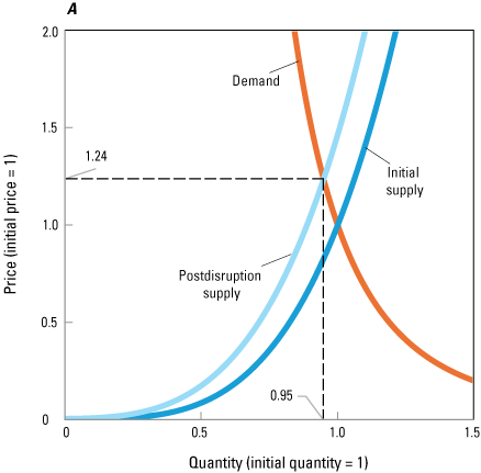
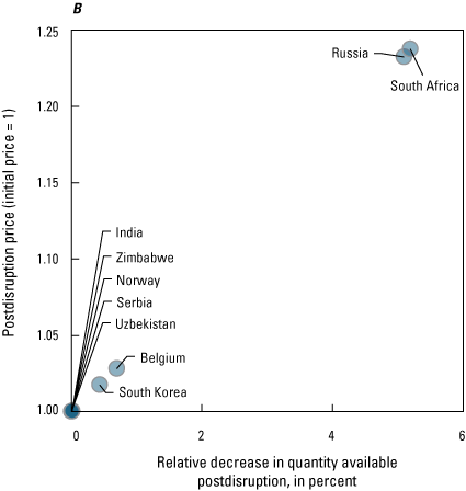
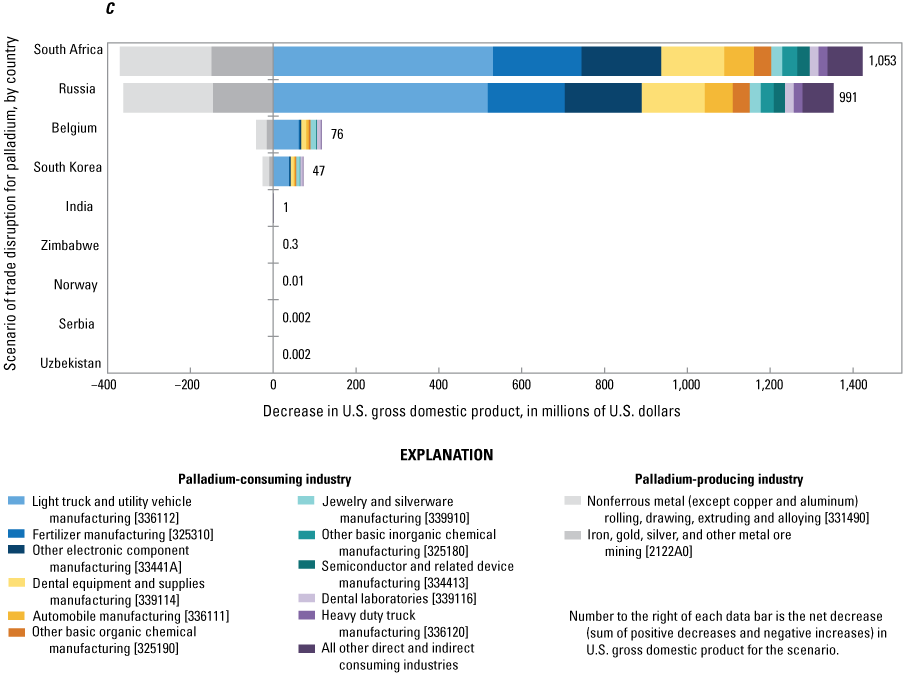
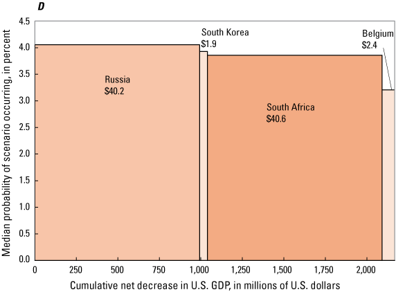
Four graphs showing various results from modeling trade disruption scenarios (the restriction of U.S. net imports from producers from which the United States was a direct or indirect net importer) for palladium. A, estimated palladium supply and demand curves for the rest of the world under a trade disruption scenario in which U.S. net imports of palladium from Russia were completely restricted for an entire year. Demand remaining constant, the supply curve shifts postdisruption, causing the postdisruption price to increase and quantity to decrease. B, estimated postdisruption price increase and relative decrease in quantity available postdisruption under nine trade disruption scenarios for palladium (the restriction of U.S. net imports of palladium from nine producers from which the United States was a direct or indirect net importer: Belgium, India, Norway, Russia, Serbia, South Africa, South Korea, Uzbekistan, and Zimbabwe). C, net decreases in U.S. gross domestic product (GDP) by industry under nine trade disruption scenarios for palladium. Industries shown are those industries that had the highest contributions to the net decrease in U.S. GDP for palladium across the nine scenarios. Each industry is followed by a 6‑character alphanumeric code from the U.S. Bureau of Economic Analysis in brackets. Values represent the effect for each scenario in current (2023) U.S. dollars, but not do reflect the probability of occurrence. Negative values indicate an increase in U.S. GDP by a given industry. Number to the right of each data bar is the net decrease (sum of positive decreases and negative increases) in U.S. GDP for the scenario. The scenarios are listed in descending order of net decrease. D, estimated median probability of scenario occurrence and net decreases in U.S. GDP for nine trade disruption scenarios for palladium. Five scenarios have net decreases too small to be legible on the figure. Probability-weighted net decreases in U.S. GDP (the product of the modeled net decrease for the scenario and its probability of occurrence) are represented as the area of each scenario with the value being displayed (in millions of U.S. dollars) below the country name for each scenario. The total area (across all scenarios) represents the overall probability-weighted net decrease in U.S. GDP for palladium. Scenarios are shown consecutively along the horizontal axis in descending order by the probability of the scenario occurring to show the relative contribution of the given scenarios to the overall probability-weighted net decrease in U.S. GDP.
Results from the economic impacts modeling for all nine palladium scenarios by industry are displayed in figure 1C. Specifically, this part of the figure displays the modeled effects on U.S. GDP for 11 palladium-consuming industries that contributed the most to the decreases along with increases to U.S. GDP from 2 palladium-producing industries (mining and recycling) and an “all other industries” category that reflects the aggregate effect on the remaining 389 industries, which includes several additional industries that were direct consumers of palladium. All changes in U.S. GDP are presented in current (2023) U.S. dollars. Scenarios of Russian and South African palladium trade disruptions resulted in the largest net decreases in U.S. GDP (displayed in the data labels of each scenario in figure 1C) of approximately $1 billion each, whereas the scenarios for Belgium and South Korea both resulted in net decreases of less than $100 million and those from the five other scenarios resulted in net decreases of $1 million or less. Although the specific industry contributions to the decreases varied by scenario, the industries that contributed the most overall were the “Light truck and utility vehicle manufacturing [336112]” industry, where palladium is used in catalytic converters; the “Fertilizer manufacturing [325310]” industry, where palladium is used as a catchment gauze in nitric acid production; and the “Other electronic components manufacturing [33441A]” industry, where palladium is used in multilayer ceramic capacitors. The other industries affected reflect palladium’s use in dental alloys, hybrid integrated circuits, jewelry, catalytic converters for other vehicle classes, and catalysts for other chemical industries. In these scenarios of foreign supply disruptions, palladium-producing industries (under BEA industry code 2122A0 for mining and 331490 for recycling) garnered higher palladium prices and increased their palladium production, thereby increasing their positive contribution to U.S. GDP, which reduced the net effect of the trade disruptions on the economy overall.
Figure 1D displays the results of the economic impacts model for each scenario (horizontal axis) and the median probability of the scenario occurring (vertical axis) based on the analysis conducted by Ryter and Nassar (2025). In this variable-width column graph, the area of each scenario (the product of the median probability and the net decrease in U.S. GDP) represents the probability-weighted net decrease in U.S. GDP. Although the South African scenario resulted in the largest decrease of U.S. GDP (as also displayed in figure 1C), its probability of occurrence (approximately 3.9 percent) was slightly lower than of the Russian scenario (approximately 4.1 percent). The probability of Russia restricting palladium supplies might seem low given recent geopolitical tensions but is attributable to the relative infrequency with which Russia imposes export restrictions on mineral commodities, which may be a reflection of their importance as a revenue source (Ryter and Nassar, 2025). Additionally, the scenarios do not account for any current or potential U.S.-imposed import sanctions. Nevertheless, the contribution of the Russian scenario (the product of the scenario’s impact and probability represented by the area of the scenario) to the overall probability-weighted net decrease in U.S. GDP was slightly smaller ($40.2 million) than that of the South African scenario ($40.6 million). The contributions to the probability-weighted net decrease in U.S. GDP from the South Korean and Belgian scenarios were both lower. Although the other 5 scenarios are displayed in figure 1D, they are too small (on the horizontal axis) to be legible. The probability-weighted net decrease in U.S. GDP across all scenarios, the entirety of the shaded area of figure 1D, totaled approximately $85 million.
Results by Trade Disruption Scenario
A summary of the contributions to the probability-weighted net decrease in U.S. GDP for each mineral commodity by leading country contribution is provided in table 1. The results indicate that samarium has the largest overall probability-weighted net decrease in U.S. GDP of nearly $4.5 billion. This modeled economic impact comes almost entirely from the China disruption scenario, for which a probability of 100 percent was used because of the recent export restriction. Several of the other “middle” and “heavy” rare earth elements (that is, lutetium, terbium, dysprosium, gadolinium, and yttrium) were also determined to have among the largest probability-weighted net decreases in U.S. GDP among all the mineral commodities examined, owing to the near complete lack of production of these mineral commodities outside of China. China was the leading contributor to the probability-weighted net decrease in U.S. GDP of 46 of the 84 mineral commodities examined, including all the rare earth elements, gallium, germanium, tungsten, and magnesium metal. Canada and South Africa were each the leading contributor to the probability-weighted net decrease in U.S. GDP for eight mineral commodities including potash, aluminum, and zinc (smelted) for Canada and rhodium, platinum, ruthenium, iridium, and chromium ferroalloys for South Africa. Most (at least 50 percent) of the contributions to the probability-weighted net decrease in U.S. GDP come from a single scenario for 65 out of the 76 mineral commodities that had positive probability-weighted net decreases in U.S. GDP—a reflection of the high degree of country-level concentration of both world production and U.S. imports.
Table 1.
Probability-weighted net decreases in U.S. gross domestic product (GDP), by scenario across all industries, and scenario contributing most to the probability-weighted net decrease in U.S. GDP for each mineral commodity.[Mineral commodities are listed in order of overall probability-weighted net decrease in U.S. GDP. Scenarios shown are the disruption of U.S. net imports of the mineral commodities from 12 producers from which the United States was a net importer that resulted in the greatest probability-weighted net decrease in U.S. GDP across the mineral commodities examined: Australia, Belgium, Brazil, Canada, Chile, China, Germany, India, Malaysia, Mexico, Russia, South Africa. All other scenarios are aggregated under the “all other countries” column. Probability-weighted net decreases are the product of the net decrease in U.S. GDP of the scenario and its median probability of occurrence. Results are in current (2023) U.S. dollars and were rounded to the nearest million U.S. dollars; may not add to totals shown. Probability-weighted net decrease values are gradationally shaded between the 5th and 95th percentiles of the values in the table to visually highlight positive (orange) to negative (blue) values. For mineral commodities with an overall negative net decrease (meaning those with an overall net increase) in U.S. GDP, the scenario contributing the most to the net decrease is not displayed. %, percent; —, indicates that the scenario was not applicable for that mineral commodity]
Summing the economic impact across mineral commodities should not be viewed as the potential effect of simultaneous disruptions across multiple mineral commodities, as such a scenario may have notably different results owing to the interactions between the industries and mineral commodities involved.
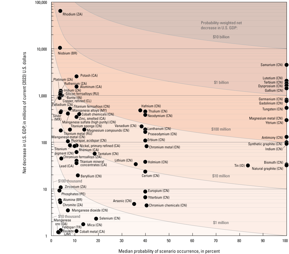
Graph showing net decreases in U.S. gross domestic product (GDP) and median probability of occurrence for the leading trade disruption scenario for 72 of the 84 mineral commodities examined. Scenarios with net decreases less than $1 million are not displayed. Vertical axis is displayed in a logarithmic scale. The gray curves are used to provide a visual reference for the resultant probability-weighted net decreases in U.S. GDP (the product of the net decrease in U.S. GDP of the scenario and its median probability) at several different orders of magnitude, and intervals between the curves are shaded to help visually group scenarios of similar magnitudes. Point labels display the mineral commodity and (where necessary) the supply chain process or chemical form, followed by the restricting country in parentheses, shown using each country's 2‑letter ISO 3166 country code, as follows: BR, Brazil; CA, Canada; CL, Chile; CN, China; GA, Gabon; ID, Indonesia; IN, India; JM, Jamaica; MX, Mexico; MY, Malaysia; PE, Peru; RU, Russia; TR, Turkey; ZA, South Africa.
If a specific disruption scenario were to take place, its impact would be greater than the probability-weighted value. For example, the modeled South African trade disruption of rhodium was estimated to result in a net decrease of over $64 billion in U.S. GDP. However, because the probability of such an occurrence is 3.9 percent, the probability-weighted decrease was just under $2.5 billion. Similarly, a niobium disruption from Brazil was estimated to result in a net decrease of over $10.4 billion in U.S. GDP, but the estimated probability of occurrence is 3.7 percent. This is more clearly displayed in figure 2, which plots the effect (net decreases) on U.S. GDP (vertical axis) and the median probability of occurrence (horizontal axis) for the leading scenario for each mineral commodity. Scenarios with net decreases less than $1 million are not displayed in figure 2. Figure 2 only displays the scenario with largest net decrease in U.S. GDP for each mineral commodity. Only one scenario is thus displayed for each mineral commodity even if that mineral commodity has more than one scenario with net decreases over $1 million. Consequently, figure 2 does not display the mineral commodity’s overall probability-weighted net decrease in U.S. GDP across all scenarios.
Results by Industry
Table 2 displays the same probability-weighted net decrease in U.S. GDP for each mineral commodity as table 1 but now by leading contributing industry. This figure highlights that samarium’s probability-weighted net decrease in U.S. GDP was mainly driven by the “Guided missile and space vehicle manufacturing [336414]” and the “Search, detection, and navigation instruments manufacturing [334511]” industries. The “Search, detection, and navigation instruments manufacturing [334511]” industry was also a notable contributor to the probability-weighted net decrease in U.S. GDP for germanium. The largest contributing industry to the probability-weighted net decrease in U.S. GDP for germanium was, however, the “Semiconductor and related device manufacturing [334413]” industry, which was also a leading contributor to the probability-weighted net decrease in U.S. GDP for gallium, lutetium, and thulium. The “Electric lamp bulb and part manufacturing [335110]” industry was the largest contributor to the probability-weighted net decrease in U.S. GDP for terbium, gadolinium, and yttrium, where these mineral commodities are used as phosphors. A large contributor to the probability-weighted net decrease in U.S. GDP decline for terbium and other rare earths used in permanent magnets (dysprosium, gadolinium, neodymium, and praseodymium) was the “Audio and video equipment manufacturing [334300]” industry.
Table 2.
Probability-weighted net decrease in U.S. gross domestic product (GDP) by industry across all scenarios, and industry contributing most to probability-weighted net decrease in U.S. GDP for each mineral commodity.[Mineral commodities are listed in order of overall probability-weighted net decrease in U.S. GDP. Only the 10 industries that contributed the most (in descending order from left to right) to the probability-weighted net decrease in U.S. GDP across all mineral commodities are displayed. The probability-weighted net decrease in U.S. GDP for the remaining 392 industries are aggregated under the “all other industries” category. Each industry name is followed by a 6-character alphanumeric code from the U.S. Bureau of Economic Analysis in brackets. Results are in current (2023) U.S. dollars and were rounded to the nearest million U.S. dollars; may not add to totals shown. Probability-weighted net decrease values are gradationally shaded between the 5th and 95th percentiles of the values in the table to visually highlight positive (orange) to negative (blue) values. mfg., manufacturing]
These results are as much a reflection of the scenarios (and the probability of each scenario’s occurrence) as they are of the importance of the mineral commodity to the identified industry. For example, neodymium and praseodymium play prominent roles in permanent magnets, perhaps more so than samarium. However, the disruption scenarios for these two rare earth elements yielded notably lower impacts than those of the other rare earth elements used in permanent magnets owing to the increased production of separated “light” rare earth elements outside of China in recent years. Similarly, lutetium has a very limited role (as a cracking catalyst) in petroleum refining, in contrast to palladium, platinum, and rhenium. The notable contribution to lutetium’s probability-weighted net decrease in U.S. GDP from that industry is thus more of a reflection of that scenario (in which virtually no lutetium production exists outside of China) than of lutetium’s importance to the petroleum refining industry. Moreover, because of extremely inelastic supply and demand, a large portion of the probability-weighted net decrease in U.S. GDP for lutetium was modeled to come from the consuming industry paying higher prices.
Results by Economic Effects Component
The effect of consuming industries paying higher prices is more clearly reflected in table 3, which summarizes the probability-weighted net decrease in U.S. GDP for the following economic effects components: consuming industries reducing their output, consuming industries paying higher prices, producing industries increasing their output, producing industries receiving higher prices, and all other industries reducing their output. Displaying the results by component highlights the role of price elasticities and the availability of excess production capacity outside of the restricting country in the analysis. Approximately one-half of samarium’s probability-weighted net decrease in U.S. GDP was due to consuming industries paying higher prices. Consuming industries paying higher prices was a major contributor to the probability-weighted net decrease in U.S. GDP for several other mineral commodities including aluminum, antimony, copper (refined), gold, lead, neodymium, potash, rhodium, silver, tungsten, and zinc (smelted). In contrast, consuming industries reducing their output was a larger contributor to the probability-weighted net decrease in U.S. GDP for most of the other mineral commodities with large probability-weighted net decreases in U.S. GDP including, dysprosium, gadolinium, gallium, germanium, hafnium, magnesium metal, niobium, terbium, and yttrium.
Table 3.
Probability-weighted net decrease in U.S. gross domestic product (GDP) by economic effects component (net decrease in U.S. GDP owing to changes in industry outputs or higher mineral commodity prices).[Mineral commodities are listed in order of overall probability-weighted net decrease in U.S. GDP. Results are in current (2023) U.S. dollars and were rounded to the nearest million U.S. dollars; may not add to totals shown. Probability-weighted net decrease values are gradationally shaded between the 5th and 95th percentiles of the values in the table to visually highlight positive (orange) to negative (blue) values. —, no domestic producers of the mineral commodity]
Table 3 also provides insights into the availability or lack of domestic production. As noted earlier, under scenarios of foreign trade disruptions, domestic producers of the mineral commodity benefit from higher prices and increased output. For all mineral commodities examined, domestic producers benefited more from higher prices than from increased output. This was especially the case for producers of aluminum, copper (refined), gold, lead, rhodium, and tungsten. For gold, the higher prices that domestic producers would be expected to receive more than offset the expected decreases in U.S. GDP attributable to lower outputs of and higher prices paid by consuming industries.
The impact on all other industries (those that are not direct consumers or producers of the mineral commodity) varies notably by mineral commodity and reflects how downstream industries may be affected. One factor that may have affected these results was whether the mineral commodity was consumed as a final good (as reflected in final demand) or was mainly an input for downstream manufacturers (as reflected in interindustry intermediate demand). Several of the mineral commodity alloys (for example, manganese alloys, silicon ferroalloys, and titanium ferroalloys) have much larger contributions to the probability-weighted net decreases in U.S. GDP from downstream industries rather than from direct consuming industries. For some mineral commodities, the contributions to the probability-weighted net decrease in U.S. GDP was negative for both the consuming industries and all other industries, reflecting a net increase in their overall economic activity. Note that these are aggregate results (across various industries and scenarios) and can be attributed to the optimization routine finding an optimal solution that allowed some industries to increase their economic activity while satisfying the specified constraints on mineral commodity availability and industry output capacity. This economic adjustment would occur when industries with relatively high contributions to U.S. GDP per unit of mineral commodity consumption increased their output while industries with lower contributions reduced their output even more, thereby reducing the overall consumption of the mineral commodity and meeting the mineral availability constraint of the scenario. These tradeoffs between industries were limited by the objective function of the optimization routine, which sought to minimize change. In practical terms, these net increases in U.S. GDP from direct and indirect consuming industries reflects the ability of industries to adjust their economic activities in response to the trade disruption scenario.
Summary of Results and Recommendations
Table 4 provides a summary of the key results (the probability-weighted net decreases in U.S. GDP for each mineral commodity examined) and recommendations for each mineral commodity’s inclusion on the LCM. The results largely reflect the following factors:
-
1. the concentration of U.S. net imports from countries likely to prohibit exports,
-
2. the size of U.S. imports as a share of production outside of the restricting country,
-
3. the import dependence of the United States,
-
4. the availability of excess capacity outside of the restricting country,
-
5. the responsiveness (elasticity) of supply and demand in the short term (within 1 year), and
-
6. the economic value of the (direct and indirect) consuming and producing industries’ contributions to the U.S. economy.
Table 4.
Overview of mineral commodity assessment, ranking, and categorization for inclusion on the draft List of Critical Minerals (LCM) in 2025.[Mineral commodities are listed in order of overall probability-weighted net decrease in U.S. gross domestic product (GDP). Mineral commodities that were not evaluated using the quantitative assessment were not ranked (ranking represented by a dash, —) and are ordered alphabetically after those ranked. Results are in current (2023) U.S. dollars and were rounded to the nearest million U.S. dollars; may not add to totals shown. Statistical risk categories were determined based on the probability-weighted net decreases in U.S. GDP (in millions of U.S. dollars) in rounded intervals, as follows: high, >206; elevated, >22 to 206; moderate, >2 to 22; limited, >0.06 to 2; negligible, 0 to 0.06; negative, <0. A mineral commodity was recommended for inclusion on the updated LCM if the probability-weighted net decrease in U.S. GDP decline was determined to be at or above the “moderate” risk category in any process of the domestic supply chain (or chemical form) or if the mineral commodity had a single point of failure (SPOF) in the supply chain. Probability-weighted net decrease values and their corresponding risk categories are shaded according to their risk category classification: high to limited are shaded in progressively lighter shades of orange; negligible are white; and negative are blue. Mineral commodity forms and supply chain processes not previously assessed separately are marked with an asterisk in the final column]
As described in the “Methods” section, statistical risk categories were determined based on the Jenks natural breaks optimization method. The results of that statistical method indicate that the probability-weighted net decreases in U.S. GDP for the 84 mineral commodities examined can be classified into five risk classes or categories (after excluding the mineral commodities with overall net increases to the probability-weighted U.S. GDP, indicated as “negative” in table 4). These risk categories, as shown in table 4, had the following descriptors and ranges of probability-weighted net decreases (in millions of current [2023] U.S. dollars): “negligible,” 0 to 0.06; “limited,” >0.06 to 2; “moderate,” >2 to 22; “elevated,” >22 to 206; and “high,” >206.
Based on the first criterion, mineral commodities are recommended be included on the updated LCM if the probability-weighted net decrease in U.S. GDP decline was found to be at or above the “moderate” risk category in any stage of the supply chain (or chemical form). With two risk categories above and two risk categories below, selecting the “moderate” risk category prevents the exclusion of mineral commodities with notable risks (those with probability-weighted net decreases in U.S. GDP in the tens of millions of current [2023] U.S. dollars) and avoids the inclusion of those with risks that are likely too low for consequential policy consideration (those with probability-weighted net decreases in U.S. GDP in the hundreds of thousands of U.S. dollars and up to $2 million). Policymakers and other users who use the LCM may, however, elect to use a different minimum risk category (for example, “elevated”) or a specific monetary cutoff value (for example, $100 million) that corresponds to a specific risk tolerance or meets the definition of “significant consequences” outlined in the Energy Act of 2020.
The second criterion was if the mineral commodity had a SPOF. Although several mineral commodities currently have a SPOF, it was only necessary to apply this criterion to zirconium given that the other mineral commodities had risk ratings categorized as being “moderate” or higher. Although there were two firms that recovered zircon—the primary source of zirconium—from heavy-mineral sands and two firms that produced zirconium metal (U.S. Geological Survey, 2025a), there was only one domestic producer of fused zircon and no domestic producer of zirconium oxychloride, both of which were necessary precursors for zirconium metal (Nassar and Fortier, 2021; U.S. Trade Representative, 2019).
In comparison to the previous LCM from 2022, several additional mineral commodities are now recommended for inclusion (in descending order of risk as determined in this assessment): potash, silicon (in particular, silicon ferroalloys), copper (in particular, refined copper), silver, rhenium, and lead. Although global potash production was not as highly concentrated as some other mineral commodities, the vast majority (approximately 90 percent) of U.S. net imports of potash were obtained from a single country, Canada, in 2023. Potash’s relatively large probability-weighted net decrease in U.S. GDP is thus principally a reflection of the high degree of U.S. dependency on Canada (refer to table 1 and fig. 2). In contrast to the low disruption probabilities for Russia and South Africa, Canada’s disruption probability for several mineral commodities is relatively high (for example, just under 11 percent for potash). This comparatively elevated probability can be attributed to Canada’s relatively high rate of historical trade barrier implementation. Between 1989 and 2023, Canada implemented prohibition, quota, or licensing requirements on mineral commodities in 8 different years, whereas other key mineral commodity-producing countries such as Russia and South Africa have implemented such barriers in only 6 and 4 different years, respectively (Ryter and Nassar, 2025). Even if the probability of a Canadian potash trade disruption scenario occurring was an order magnitude lower than estimated (for example, 1.1 percent instead of 11 percent), the overall probability-weighted net decrease in U.S. GDP for potash would still be considerably higher (around $41 million after accounting for not only the assumed lower probability for the Canadian scenario but also all the other scenarios at the estimated probabilities) than the minimum value required to meet the “moderate” risk category of greater than $2 million. Silver’s probability-weighted net decrease in U.S. GDP is largely due to a scenario in which Mexico stops silver exports to the United States—a high impact ($435 million), low probability (4 percent) event (refer to table 1 and fig. 2). In the previous LCM assessment (Nassar and Fortier, 2021), lead and rhenium were both just below the cutoff threshold for recommendation to the LCM, whereas the risk for refined copper was trending upward. The evaluation of lead and rhenium just above the minimum threshold of this assessment underscores the idea that risk assessments operate on a continuum. Evaluating a mineral commodity just above and subsequently just below a threshold in consecutive assessments may also warrant the retention of the mineral commodity on the LCM for additional time to allow for stability in policymaking. Silicon metal and mined copper have negative probability-weighted net decreases in U.S. GDP but are still recommended for inclusion because of the risks associated with other stages of their supply chains, namely silicon ferroalloys and refined copper. Their negative probability-weighted net decreases in U.S. GDP were due to the United States being a net exporter of copper ores and concentrates and exporting higher value (and higher grades of) silicon metal (polysilicon) than it imports.
Arsenic and tellurium, both of which were included on the previous LCM in 2022, do not qualify under either criterion of this assessment. With the recent installation of copper telluride recovery capability by a major copper operation in Utah (Rio Tinto plc, 2022), the United States has moved from being over 95 percent net import reliant in 2021 to being a net exporter of tellurium in 2023 (U.S. Geological Survey, 2025a). Although the domestically produced copper telluride was not refined in the United States, the notable reduction of U.S. imports of tellurium since 2022 (U.S. Geological Survey, 2025a) has resulted in a decrease in tellurium’s supply risk from foreign trade disruptions. However, that risk may return if one or both current domestic producers stop recovering copper telluride or if world tellurium production becomes even more geopolitically concentrated despite the notable enrichment (but lack of recovery) of tellurium within the copper anode slimes of copper electrolytic refineries (Nassar and others, 2022). Although the United States obtains most of its arsenic from China, revised data from the USGS (U.S. Geological Survey, 2025b) indicates that Peru (not China) was the leading producer of arsenic. Even though arsenic remains important for its use in gallium arsenide wafers, a greater concern in that supply chain is China’s dominance in primary gallium production (Nassar and others, 2024).
As with the previous LCM assessment, there were insufficient data to quantitatively evaluate the risks for cesium, rubidium, and scandium. Although they have limited commercial applications, the United States has continued to be completely import reliant for all three mineral commodities (U.S. Geological Survey, 2025a). Moreover, scandium is specifically called out for export restriction by China’s MOFCOM (Ministry of Commerce of the People’s Republic of China, 2025b). There was insufficient justification for changing their status on the LCM, but future assessments could strive to quantitively assess their risk.
Conclusions
The results of the economic effects assessment and the SPOF criteria recommend the addition of six mineral commodities (in descending risk order, potash, silicon, copper, silver, rhenium, and lead) to the LCM and the removal of two mineral commodities (arsenic and tellurium) from the LCM. These recommendations are based on a statistical approach that classifies the probability-weighted economic effects into specific quantitative intervals. In determining the final LCM or in using the results of this methodology, decisionmakers may wish to consider other thresholds based on a specific risk tolerance, examine other risks (for example, the potential for supply disruptions from natural hazards [Jaiswal and others, 2024]), or address other considerations (for example, future demand expectations or the strategic importance of certain industries beyond economic valuation). Moreover, although defense-related industries are captured in the IO tables, consequences to the national security of the United States beyond economic effects are not directly factored into this analysis but may be addressed in the final LCM through consultation with the heads of other relevant executive departments and agencies as indicated by the Energy Act of 2020. Additionally, postponing the removal of mineral commodities may provide sufficient time for current policies to achieve their intended effects. For example, the Secretary of the Interior may decide to remove a mineral commodity now or wait to see if it is again recommended for removal in the next cycle. The assessment of risk exists on a continuum and this may influence decisions for mineral commodities near thresholds of evaluation. Mineral commodities with the highest probability-weighted net decreases in U.S. GDP may warrant closer evaluation and prompt greater attention from policymakers and other users of this information than those with low or negative probability-weighted net decreases in U.S. GDP. Several of the mineral commodities with the highest estimated risk have not only received attention but also action by the U.S. Government and others. For example, earlier this year, an Australian company’s facility in Malaysia announced plans to expand its heavy rare earth separation circuit to produce dysprosium, holmium, and terbium concentrate (Govind, 2025) and has plans to build a plant with similar capabilities in the United States through Presidential directive under Defense Production Act Title III (U.S. Department of Defense, 2021). Additionally, a U.S. producer recently announced that it has entered a partnership with the U.S. Department of Defense to accelerate its U.S. rare earth mine-to-magnet supply chain (MP Materials Corp., 2025). These recent announcements are part of a years-long effort on the part of the U.S. Government and other governments around the world aimed at reducing the risks associated with rare earths and other critical mineral commodities (International Energy Agency, 2025).
By performing an economic effects assessment, the results of this analysis can be used to provide a direct quantitative comparison of mineral commodities against each other and also to other risks and priorities. These results also allow for the performance of cost-benefit analyses of various risk mitigation strategies (for example, maintaining a stockpile, securing trade agreements, developing substitute materials, or increasing domestic primary or secondary production [Nassar and others, 2020]). Policymakers may, for example, consider whether the annualized costs of a specific risk mitigation strategy are determined to be greater or less than the expected risks noted here as part of their decision-making process. Moreover, it might not be cost-effective to address all the mineral commodities that are on the LCM. For example, europium and ytterbium are both just above the selected statistical threshold with probability-weighted net decreases in U.S. GDP of $3.5 million and $2.6 million, respectively. Neither europium nor ytterbium were evaluated quantitatively in the last LCM assessment. Instead, their assessment was based on a qualitative evaluation. Although supply chains of both rare earth elements are still dominated by China, their limited use in the United States reduces the potential economic impact of any expected trade disruption. Europium’s use in phosphors for lighting and displays, for example, has decreased notably over the past decade (Wang and others, 2020). It may therefore not be cost-effective to focus risk mitigation efforts on these mineral commodities given that the expected economic effects are not very high. In interpreting the results, note that the probability-weighted net decreases in U.S. GDP are not the same as what the effects would be if a specific event were to occur. Moreover, the effects of prolonged mineral commodity trade restrictions are not captured in the 1-year-long scenarios of this analysis.
As noted in the previous LCM assessment (Nassar and Fortier, 2021), no single analysis can alone capture all the intricacies and nuances of the complex global supply chains of these mineral commodities. Moreover, data limitations, especially on the consumption of certain mineral commodities by application and industry, introduce uncertainty to the analysis that is difficult to quantify. Additionally, the results reflect the assumptions and simplifications made in both the scenarios and the models—some of which may not hold. For example, the extraterritorial enforcement of export restrictions is already reportedly being circumvented for some mineral commodities, like antimony, on which China has placed export restrictions (Parodi and others, 2025). Furthermore, scenario probabilities were estimated using machine-learning classifiers with data on prior official Government policies associated with export restrictions that cannot perfectly predict future actions (Ryter and Nassar, 2025). Other simplifications (for example, the streamlined IO table expansion approach) and assumptions (for example, the use of constant price elasticities) may affect the results in ways that would be difficult to anticipate. Nevertheless, the results presented in this report provide several notable improvements in terms of both methods (for example, the use of economic models) and scope (for example, the inclusion of several additional mineral commodity forms) compared with previous assessments. Moreover, although the analysis presented here shares a similar conceptual framework with the previous LCM assessment (Nassar and Fortier, 2021), it did not directly use any of the same indicators or methods. For example, neither the world production concentration nor the U.S. net import reliance indicators of the previous assessment were direct inputs in this analysis. Despite the methodological differences, the results of the two assessments largely overlap, which may provide a certain level of reassurance in the conclusions. While retaining the same conceptual framework, future work could continue to improve the analysis by collecting more comprehensive data, addressing model simplifications and assumptions, and expanding the scope to include other mineral commodities and scenarios.
References Cited
Board of Governors of the Federal Reserve System, 2024, Industrial production and capacity utilization—G.17: Federal Reserve System web page, accessed November 7, 2024, at https://www.federalreserve.gov/releases/g17/caputl.htm.
CVXPY, 2025, CVXPY 1.6.5: CVXPY software release, accessed July 11, 2025, at https://www.cvxpy.org/.
Fortier, S.M., Nassar, N.T., Lederer, G.W., Brainard, J., Gambogi, J., and McCullough, E.A., 2018, Draft critical mineral list—Summary of methodology and background information—U.S. Geological Survey technical input document in response to Secretarial Order No. 3359: U.S. Geological Survey Open-File Report 2018–1021, 15 p., https://doi.org/10.3133/ofr20181021.
Goulart, P.J., and Chen, Y., 2024, Clarabel—An interior-point solver for conic programs with quadratic objectives: arXiv, preprint posted May 21, 2024, 48 p., accessed July 10, 2025, at http://arxiv.org/abs/2405.12762.
Govind, A., 2025, Australia’s Lynas produces terbium oxide in Malaysia: Argus Media group web page, accessed July 14, 2025, at https://www.argusmedia.com/en/news-and-insights/latest-market-news/2700216-australia-s-lynas-produces-terbium-oxide-in-malaysia.
International Energy Agency, 2025, Critical minerals policy tracker: International Energy Agency website, accessed July 14, 2025, at https://www.iea.org/data-and-statistics/data-tools/critical-minerals-policy-tracker.
International Trade Administration, 2015, Trade data basics: International Trade Administration web page, accessed July 14, 2025, at https://legacy.trade.gov/mas/ian/referenceinfo/tg_ian_001872.asp.
Jaiswal, K.S., Luco, N., Schnebele, E.K., Nassar, N.T., and Otarod, D., 2024, Quantitative risk of earthquake disruption to global copper and rhenium supply: U.S. Geological Survey Open-File Report 2024–1028, 19 p., accessed July 10, 2025, at https://doi.org/10.3133/ofr20241028.
Ministry of Commerce of the People’s Republic of China, 2024, Announcement No. 46 of 2024 of the Ministry of Commerce on strengthening export control of relevant dual-use items to the United States: Ministry of Commerce of the People’s Republic of China policy release, December 3, 2024, accessed July 11, 2025, at https://www.mofcom.gov.cn/zwgk/zcfb/art/2024/art_3d5e990b43424e60828030f58a547b60.html. [In Chinese.]
Ministry of Commerce of the People’s Republic of China, 2025a, Announcement No. 10 of 2025 of the Ministry of Commerce and the General Administration of Customs on the decision to implement export control on items related to tungsten, tellurium, bismuth, molybdenum and indium: Ministry of Commerce of the People’s Republic of China policy release, February 4, 2025, accessed July 11, 2025, at https://www.mofcom.gov.cn/zwgk/zcfb/art/2025/art_e623090907fc4e1092f0a4db72f57b95.html. [In Chinese.]
Ministry of Commerce of the People’s Republic of China, 2025b, The Ministry of Commerce and the General Administration of Customs announced in Announcement No. 18 of 2025 the decision to implement export controls on some medium and heavy rare earth related items: Ministry of Commerce of the People’s Republic of China news release, April 9, 2025, accessed July 11, 2025, at https://www.mofcom.gov.cn/jmxw/art/2025/art_a2284b3f7b8f4a59a6374f2009d5e36b.html.
MP Materials Corp., 2025, MP Materials announces transformational public-private partnership with the Department of Defense to accelerate U.S. rare earth magnet independence: MP Materials Corp. news release, July 10, 2025, accessed July 14, 2025, at https://investors.mpmaterials.com/investor-news/news-details/2025/MP-Materials-Announces-Transformational-Public-Private-Partnership-with-the-Departme nt-of-Defense-to-Accelerate-U-S--Rare-Earth-Magnet-Independence/default.aspx.
Nassar, N.T., Alonso, E., and Brainard, J., 2020, Investigation of U.S. Foreign Reliance on Critical Minerals—U.S. Geological Survey Technical Input Document in Response to Executive Order No. 13953 Signed September 30 (Ver. 1.1, December 7, 2020): U.S. Geological Survey Open-File Report 2020–1127, 37 p., accessed July 10, 2025, at https://doi.org/10.3133/ofr20201127.
Nassar, N.T., and Fortier, S.M., 2021, Methodology and technical input for the 2021 review and revision of the U.S. Critical Minerals List: U.S. Geological Survey Open-File Report 2021–1045, 31 p., accessed July 10, 2025, at https://doi.org/10.3133/ofr20211045.
Nassar, N.T., Kim, H., Frenzel, M., Moats, M.S., and Hayes, S.M., 2022, Global tellurium supply potential from electrolytic copper refining: Resources, Conservation and Recycling, v. 184, p. 106434, accessed July 10, 2025, at https://doi.org/10.1016/j.resconrec.2022.106434.
Nassar, N.T., Pineault, D., Allen, S.M., McCaffrey, D.M., Padilla, A.J., Brainard, J.L., Bayani, M., Shojaeddini, E., Ryter, J.W., Lincoln, S., Alonso, E., 2025, Appendices for “Methodology and Technical Input for the 2025 U.S. List of Critical Minerals—Assessing the Potential Effects of Mineral Commodity Supply Chain Disruptions on the U.S. Economy”: Zenodo, preprint posted August 25, 2025, 233 p., accessed August 25, 2025, at https://doi.org/10.5281/zenodo.16538520.
Nassar, N.T., Shojaeddini, E., Alonso, E., Jaskula, B., and Tolcin, A., 2024, Quantifying potential effects of China’s gallium and germanium export restrictions on the U.S. economy: U.S. Geological Survey Open-File Report 2024–1057, 66 p., accessed October 15, 2024, at https://doi.org/10.3133/ofr20241057.
Oosterhaven, J., and Bouwmeester, M.C., 2016, A new approach to modeling the impact of disruptive events: Journal of Regional Science, v. 56, no. 4, p. 583–595, accessed July 30, 2024, at https://doi.org/10.1111/jors.12262.
Parodi, A., Jackson, L., Shivaprasad, A., and Varghese, S.E., 2025, How US buyers of critical minerals bypass China’s export ban: Thomson Reuters, July 9, 2025, accessed July 9, 2025, at https://www.reuters.com/business/autos-transportation/how-us-buyers-critical-minerals-bypass-chinas-export-ban-2025-07-09/.
Python Software Foundation, 2024, Python 3.11.8: Python Software Foundation, software release, February 6, 2024, accessed February 6, 2024, at https://www.python.org/downloads/release/python-3118/.
Rio Tinto plc, 2022, Rio Tinto starts tellurium production at Kennecott: Rio Tinto plc, news release, May 11, 2022, accessed June 26, 2025, at https://www.riotinto.com/en/news/releases/2022/rio-tinto-starts-tellurium-production-at-kennecott.
Satopaa, V., Albrecht, J., Irwin, D., and Raghavan, B., 2011, Finding a “Kneedle” in a haystack—Detecting knee points in system behavior, in 2011 31st International Conference on Distributed Computing Systems Workshops, Minneapolis, Minn. June 20–24, 2011: Institute of Electrical and Electronics Engineers, p. 166–171.
Shojaeddini, E., Alonso, E., Nassar, N.T., Pineault, D.G., Allen, S.M., Brainard, J.L., McCaffrey, D.M., O’Brien, T.M., Padilla, A.J., and Ryter, J.W., 2025, Understanding market sensitivity—Estimation of supply and demand elasticities for non-fuel minerals: Mineral Economics, accessed September 11, 2025, at https://doi.org/10.1007/s13563-025-00537-3.
U.S. Bureau of Economic Analysis, 2025, Input-output: U.S. Bureau of Economic Analysis interactive data tables, accessed July 7, 2025, at https://www.bea.gov/itable/input-output.
U.S. Census Bureau, 2020, EC1700NAPCSINDPRD—All sectors—Industry by products for the U.S. and States—2017: U.S. Census Bureau data, accessed July 23, 2024, at https://data.census.gov/table/ECNNAPCSIND2017.EC1700NAPCSINDPRD.
U.S. Census Bureau, 2022, 2018–2021 Annual Survey of Manufactures (ASM)—Tables: U.S. Census Bureau data, accessed October 11, 2023, at https://www.census.gov/data/tables/time-series/econ/asm/2018-2021-asm.html.
U.S. Census Bureau, 2024, North American Industry Classification System: U.S. Census Bureau, accessed July 20, 2025, at https://www.census.gov/naics/.
U.S. Department of Defense, 2021, DOD announces rare earth element award to strength domestic industrial base: U.S. Department of Defense news release, February 1, 2021, accessed July 14, 2025, at https://www.defense.gov/News/Releases/Release/Article/2488672/dod-announces-rare-earth-element-award-to-strengthen-domestic-industrial-base/.
U.S. Geological Survey, 2025a, Mineral commodity summaries 2025 (ver. 1.2, March 2025): U.S. Geological Survey, 212 p., https://doi.org/10.3133/mcs2025.
U.S. Geological Survey, 2025b, U.S. Geological Survey Minerals Yearbook data for select mineral commodities referenced in U.S. Geological Survey “Methodology and Technical Input for the 2025 U.S. List of Critical Minerals—Assessing the Potential Effects of Mineral Commodity Supply Chain Disruptions on the U.S. Economy”: U.S. Geological Survey data release, https://doi.org/10.5066/P14BRF29.
U.S. Trade Representative, 2019, Section 301 tariffs public hearing: U.S. Trade Representative, June 19, 2019, accessed April 9, 2021, at https://ustr.gov/sites/default/files/enforcement/301Investigations/Section_301_Hearing_Transcript_on_Proposed_Tariffs_Day_3.pdf.
Wang, Q.-C., Wang, P., Qiu, Y., Dai, T., and Chen, W.-Q., 2020, Byproduct surplus—Lighting the depreciative europium in China’s rare earth boom: Environmental Science & Technology, v. 54, no. 22, p. 14686–14693, accessed July 7, 2025, at https://doi.org/10.1021/acs.est.0c02870.
Zen Innovations AG, 2025, Global trade tracker: Zen Innovations AG, accessed January 2, 2025, at https://www.globaltradetracker.com/.
Appendixes
-
• Appendix 1. World production and production capacity data
-
• Appendix 2. U.S. trade data of mineral commodities
-
• Appendix 3. Prices and price elasticities of supply and demand
-
• Appendix 4. Mineral commodity consumption by application and associated industry
-
• Appendix 5. Python implementation of the economic impacts model
-
• Appendix 6. Natural breaks classification
Reference Cited
Nassar, N.T., Pineault, D., Allen, S.M., McCaffrey, D.M., Padilla, A.J., Brainard, J.L., Bayani, M., Shojaeddini, E., Ryter, J.W., Lincoln, S., Alonso, E., 2025, Appendices for “Methodology and Technical Input for the 2025 U.S. List of Critical Minerals—Assessing the Potential Effects of Mineral Commodity Supply Chain Disruptions on the U.S. Economy”: Zenodo, preprint posted August 25, 2025, 233 p., accessed August 25, 2025, at https://doi.org/10.5281/zenodo.16538520.
Appendix 1. World Production and Production Capacity Data
Table 1.1.
Data sources for world mineral commodity primary production and secondary production.[~, approximately; —, not applicable or not available; BEA, U.S. Bureau of Economic Analysis; Al2O3, aluminum oxide; K2O, potassium oxide; MgO, magnesium oxide; P2O5, phosphorus pentoxide; SrSO4, strontium sulfate; TiO2, titanium dioxide; ZrO2, zirconium oxide]
| Mineral commodity | Primary production | Secondary production | ||||||
|---|---|---|---|---|---|---|---|---|
| Description | Data sources | Associated BEA industry [code] | Comments | Description | Data sources | Associated BEA industry [code] | Comments | |
| Alumina | Refinery production | U.S. Geological Survey (2025a, b) | Alumina refining and primary aluminum production [331313] | Quantities were converted to aluminum content based on the standard stoichiometric ratio (~52.9‑percent aluminum). | — | — | — | — |
| Aluminum | Smelter production | U.S. Geological Survey (2025a, b) | Alumina refining and primary aluminum production [331313] | Quantities were reported in aluminum content by U.S. Geological Survey (2025a, b). | Secondary aluminum production, old scrap only | World Bureau of Metal Statistics (2022); U.S. Geological Survey (2025a) | Secondary smelting and alloying of aluminum [331314] | U.S. secondary production data were obtained from the Mineral Commodity Summaries 2025 (U.S. Geological Survey, 2025a). Data for all other countries were obtained from the World Bureau of Metal Statistics (2022), which pertained to 2021 but were assumed to be similar in 2023. |
| Antimony | Refinery production of metal (salable ingot) and antimony trioxide | Project Blue (2024a) | Nonferrous metal (except aluminum) smelting and refining [331410] | Quantities were reported in antimony content by Project Blue (2024a). | — | — | — | Although antimonial lead was recovered from spent lead-acid batteries, this secondary source was largely performed in a closed-loop fashion (Project Blue, 2024a) and was thus excluded from the analysis. Antimony oxide may also have been recovered at the end-of-life, but those quantities were estimated to be small relative to the total quantity of world production and thus assumed to be negligible (Project Blue, 2024a). |
| Arsenic | Arsenic compound production | U.S. Geological Survey (2025b) | Other nonmetallic mineral mining and quarrying [2123A0] | Quantities, which were reported in arsenic trioxide equivalent, were converted to arsenic content based on the standard stoichiometric ratio (75.7‑percent arsenic). | — | — | — | — |
| Barite | Mine production | U.S. Geological Survey (2025b) | Other nonmetallic mineral mining and quarrying [2123A0] | Quantities were converted to barium content based on the standard stoichiometric ratio (58.8‑percent barium). | — | — | — | — |
| Bauxite | Mine production | U.S. Geological Survey (2025a, b) | Iron, gold, silver, and other metal ore mining [2122A0] | Quantities were converted to aluminum content based on Al2O3 content of bauxite ore grades reported in Liu and Müller (2013) and the standard stoichiometric ratio (~52.9‑percent aluminum). For countries not
included in Liu and Müller (2013), the Al2O3 content of bauxite was assumed to be 41 percent. U.S. production was withheld by U.S. Geological Survey (2025a, b) to avoid disclosing proprietary information but was included in the analysis. |
— | — | — | — |
| Beryllium | Mine production | U.S. Geological Survey (2025a) | Other nonmetallic mineral mining and quarrying [2123A0] | In addition to the countries listed by U.S. Geological Survey (2025a), Kazakhstan was believed to have produced beryllium metallurgical products from stockpiles of concentrates (Beryllium Science & Technology Association, 2024). Kazakhstan’s production was thus estimated assuming its beryllium metallurgical product production (U.S. Geological Survey, 2025b) was 4‑percent beryllium content. Production from all other countries was reported in beryllium content. | — | — | — | — |
| Bismuth | Refinery production | U.S. Geological Survey (2025a) | Nonferrous metal (except aluminum) smelting and refining [331410] | Quantities were reported in bismuth content by U.S. Geological Survey (2025a). | — | — | — | The minor quantities (approximately 40 metric tons) of bismuth that were recycled were thought to be new scrap and thus excluded from the analysis (U.S. Geological Survey, 2025a). |
| Cadmium | Refinery production | U.S. Geological Survey (2025a) | Nonferrous metal (except aluminum) smelting and refining [331410] | Quantities were reported in cadmium content by U.S. Geological Survey (2025a). | — | — | — | Although cadmium was recovered from spent consumer and industrial batteries and other sources, no reliable country-level information was available, except for the United States, which was included in the analysis. |
| Chromite | Mine production | U.S. Geological Survey (2025b) | Iron, gold, silver, and other metal ore mining [2122A0] | Quantities were converted to chromium content based on values reported by Nassar and others (2020). | — | — | — | — |
| Chromium chemicals | Production of chromium chemicals | Project Blue (2025a) | Other basic inorganic chemical manufacturing [325180] | Quantities were converted from sodium dichromate equivalent to chromium content based on the standard stoichiometric ratio (~34.9‑percent chromium). | — | — | — | — |
| Chromium ferroalloys | Ferrochromium production (high-, medium- and low-carbon alloys) | Project Blue (2025a) | Nonferrous metal (except aluminum) smelting and refining [331410] | Quantities were reported in chromium content by Project Blue (2025a). | — | — | — | Chromium is mainly recycled in the form of stainless-steel scrap, which was excluded from this analysis. |
| Chromium metal | Production of chromium metals | Project Blue (2025a) | Nonferrous metal (except aluminum) smelting and refining [331410] | Quantities were reported in chromium content by Project Blue (2025a). | — | — | — | No reliable estimates of chromium metal recycled by country were available. |
| Cobalt chemicals | Refinery production of cobalt chemicals and fine powders | Darton Commodities Ltd. (2025) | Other basic inorganic chemical manufacturing [325180] | Quantities were reported in cobalt content by Darton Commodities Ltd. (2025). | — | — | — | — |
| Cobalt metal | Refinery production of cobalt metal and coarse powder | Darton Commodities Ltd. (2025) | Nonferrous metal (except aluminum) smelting and refining [331410] | Quantities were reported in cobalt content by Darton Commodities Ltd. (2025). | Secondary production | Darton Commodities Ltd. (2025); U.S. Geological Survey (2025a) | Nonferrous metal (except copper and aluminum) rolling, drawing, extruding and alloying [331490] | U.S. secondary production of cobalt was obtained from the U.S. Geological Survey (2025a). The rest of the world’s secondary production was estimated based on the difference between the total secondary cobalt production obtained from Darton Commodities Ltd. (2025) and the quantity of U.S. secondary cobalt production. Owing to a lack of better information, this remaining quantity was allocated to several countries (Belgium, Canada, China, Finland, France, Japan, Norway, South Korea, and the United Kingdom) based on their reported cobalt refinery capacity. |
| Copper, mined | Mine production | U.S. Geological Survey (2025a, b) | Copper, nickel, lead, and zinc mining [212230] | Quantities were reported in copper content by the reference. | — | — | — | — |
| Copper, refined | Primary refinery production | U.S. Geological Survey (2025a, b) | Nonferrous metal (except aluminum) smelting and refining [331410] | Quantities were reported in copper content by the reference. | Secondary refinery production | U.S. Geological Survey (2025a, b) | Copper Rolling, Drawing, Extruding, and Alloying [331420] | Quantities were reported in copper content by the reference. For the United States, secondary production was set equal to the quantity of copper recovered from old (post-consumer) scrap. |
| Feldspar | Feldspar mine production | U.S. Geological Survey (2025b) | Other nonmetallic mineral mining and quarrying [2123A0] | Quantities were not adjusted for any feldspar content. Nepheline syenite mine production was excluded if readily identifiable in the reported data. | — | — | — | — |
| Fluorspar, acidspar | Acid-grade fluorspar (acidspar) production | Project Blue (2025b) | Other nonmetallic mineral mining and quarrying [2123A0] | Quantities were assumed to be 47.7‑percent fluorine content. | — | — | — | — |
| Fluorspar, metspar | Metallurgical-grade fluorspar (metspar) production | Project Blue (2025b) | Other nonmetallic mineral mining and quarrying [2123A0] | Quantities were assumed to be 45.7‑percent fluorine content. | — | — | — | — |
| Gallium | Low-purity refinery production | U.S. Geological Survey (2025b) | Nonferrous metal (except aluminum) smelting and refining [331410] | Quantities were reported in gallium content by U.S. Geological Survey (2025b). | — | — | — | End-of-life recycling was assumed to be negligible. New scrap recycling was excluded from the analysis. |
| Germanium | Refinery production | Nassar and others (2024) | Nonferrous metal (except aluminum) smelting and refining [331410] | Quantities were updated to reflect production quantities in 2023 based on the same sources and methods used by Nassar and others (2024). Quantities were reported in germanium content by Nassar and others (2024). | — | — | — | End-of-life recycling was assumed to be negligible. New scrap recycling was excluded from the analysis. |
| Gold | Mine production | U.S. Geological Survey (2025b) | Iron, gold, silver, and other metal ore mining [2122A0] | Quantities were reported in gold content by U.S. Geological Survey (2025b). | Old scrap gold recycling | World Gold Council (2024) | Nonferrous metal (except copper and aluminum) rolling, drawing, extruding and alloying [331490] | Quantities, which were only reported by the World Gold Council (2024) as a total for the world, were disaggregated by country, assuming the same relative contribution of each country as reported by Alexander and others (2019) for 2018. Quantities were reported in gold content by the World Gold Council (2024). |
| Graphite, natural | Natural graphite production | U.S. Geological Survey (2025b) | Other nonmetallic mineral mining and quarrying [2123A0] | All quantities were assumed to be reported in graphite content. | — | — | — | — |
| Graphite, synthetic | Synthetic graphite production | Benchmark Mineral Intelligence Ltd. (2023) | Other petroleum and coal products manufacturing [324190] | All quantities were assumed to be reported in graphite content. | — | — | — | — |
| Hafnium | Refinery production | Mordor Intelligence (2024) | Nonferrous metal (except aluminum) smelting and refining [331410] | All quantities were reported in hafnium content. | — | — | — | — |
| Helium | Grade-A and gaseous helium | U.S. Geological Survey (2025a) | Industrial gas manufacturing [325120] | Quantities were assumed to be reported in helium content. U.S. quantities included those extracted from natural gas, as well as those withdrawn from storage. | — | — | — | — |
| Indium | Refinery production | U.S. Geological Survey (2025b) | Nonferrous metal (except aluminum) smelting and refining [331410] | Quantities were reported in indium content by U.S. Geological Survey (2025b). | — | — | — | Although there were notable quantities of new scrap recycling of indium (especially of indium-tin-oxide), end-of-life recycling of indium was assumed to be negligible. |
| Iridium | Mine production | U.S. Geological Survey (2025b) | Iron, gold, silver, and other metal ore mining [2122A0] | Quantities were reported in iridium content by U.S. Geological Survey (2025b). Additionally, U.S. mine production was estimated separately based on palladium mine production multiplied by the iridium-to-palladium ratio reported by Naldrett (2011). | End-of-life recycling | Refer to the comment | Nonferrous metal (except copper and aluminum) rolling, drawing, extruding and alloying [331490] | Closed-loop recycling of iridium from industrial applications (chemical catalysts and electrochemical applications) was excluded. Non-closed loop end-of-life recycling was estimated using the method described by Nassar (2015) and data from Johnson Matthey plc (2024). The quantity that was estimated to be recycled at the end-of-life was allocated to individual countries based on the same proportions as platinum recycling. |
| Iron ore | Mine production, as well as alternative iron ore sources including nickeliferous iron ore and titaniferous magnetite beach sands | U.S. Geological Survey (2025b) | Iron, gold, silver, and other metal ore mining [2122A0] | Quantities were reported in iron content by U.S. Geological Survey (2025b). | — | — | — | — |
| Lead | Primary refined production | U.S. Geological Survey (2025b) | Nonferrous metal (except aluminum) smelting and refining [331410] | Quantities were reported in lead content by U.S. Geological Survey (2025b). | Secondary refined production | U.S. Geological Survey (2025b) | Nonferrous metal (except copper and aluminum) rolling, drawing, extruding and alloying [331490] | Quantities were reported in lead content by U.S. Geological Survey (2025b). |
| Lithium | Refined lithium production | Project Blue (2025c) | Other basic inorganic chemical manufacturing [325180] | Quantities were converted from lithium-carbonate equivalent to lithium content based on the standard stochiometric ratio (18.8‑percent lithium). | — | — | — | The minor quantities of lithium recycled at the end-of-life (Project Blue, 2025c) were excluded owing to a lack of country-level data. |
| Magnesium compounds | Magnesite and seawater and brine production | U.S. Geological Survey (2025b) | Other basic inorganic chemical manufacturing [325180] | Quantities, which were reported in MgO equivalent, were converted to magnesium content
using the standard stochiometric ratio (60.35‑percent magnesium). Magnesium compounds from seawater and brines were estimated from production capacity quantities, as reported by U.S. Geological Survey (2025b), multiplied by an assumed 80‑percent capacity utilization rate. |
— | — | — | — |
| Magnesium metal | Primary production | U.S. Geological Survey (2025b) | Nonferrous metal (except aluminum) smelting and refining [331410] | Quantities were reported in magnesium content by U.S. Geological Survey (2025b). | Secondary production | Project Blue (2025d); U.S. Geological Survey (2025b) | Nonferrous metal (except copper and aluminum) rolling, drawing, extruding and alloying [331490] | Secondary magnesium production for the United States was based on quantity recovered from old scrap only as reported by the U.S. Geological Survey (2025b). Secondary production for all other countries was obtained from Project Blue (2025d). |
| Manganese alloys | Refinery production of high-carbon ferromanganese, medium- and low-carbon ferromanganese, and silicomanganese | Project Blue (2025e) | Iron and steel mills and ferroalloy manufacturing [331110] | Quantities were reported in manganese content by Project Blue (2025e). | — | — | — | — |
| Manganese dioxide | Refinery production | Project Blue (2024b) | Other basic inorganic chemical manufacturing [325180] | Quantities were reported in manganese content by Project Blue (2024b). | — | — | — | — |
| Manganese metal | Electrolytic or aluminothermic manganese metal production | Project Blue (2025e) | Iron and steel mills and ferroalloy manufacturing [331110] | Quantities were reported in manganese content by Project Blue (2025e). | — | — | — | — |
| Manganese ore | Mine production | International Manganese Institute (2024) | Other nonmetallic mineral mining and quarrying [2123A0] | Quantities were reported in manganese content by International Manganese Institute (2024). | — | — | — | — |
| Manganese sulfate (high purity) | Refinery production of battery-grade manganese sulfate | Project Blue (2025e) | Other basic inorganic chemical manufacturing [325180] | Quantities were reported in manganese content by Project Blue (2025e). | — | — | — | — |
| Mica | Mine (scrap and flake) production | U.S. Geological Survey (2025b) | Other nonmetallic mineral mining and quarrying [2123A0] | Quantities were not adjusted for any elemental content. Production excludes sheet mica where it is distinguishable in the data. | — | — | — | — |
| Molybdenum | Mine production | U.S. Geological Survey (2025b) | Iron, gold, silver, and other metal ore mining [2122A0] | Quantities were reported in molybdenum content by U.S. Geological Survey (2025b). | — | — | — | Molybdenum is recycled in notable quantities in the form of spent catalysts, ferrous scrap, and superalloy revert. No recent production quantities were available, and thus secondary production was excluded from the analysis. |
| Nickel, mined | Mine production | U.S. Geological Survey (2025b) | Copper, nickel, lead, and zinc mining [212230] | Quantities were reported in nickel content by U.S. Geological Survey (2025b). | — | — | — | — |
| Nickel, primary refined | Primary refinery production | U.S. Geological Survey (2025b) | Nonferrous metal (except aluminum) smelting and refining [331410] | Quantities were reported in nickel content by U.S. Geological Survey (2025b). | — | — | — | Nickel is extensively recycled, especially in the form of stainless-steel scrap. Because of this, the focus of this analysis is on primary refined nickel only. |
| Niobium | Mine production | U.S. Geological Survey (2025b) | Iron, gold, silver, and other metal ore mining [2122A0] | Quantities were reported in niobium content by U.S. Geological Survey (2025b). | — | — | — | Niobium recycling does take place, but specific recycling quantities were not available. |
| Palladium | Mine production | U.S. Geological Survey (2025b) | Iron, gold, silver, and other metal ore mining [2122A0] | Quantities were reported in palladium content by U.S. Geological Survey (2025b). | Automotive catalytic converter, jewelry, and electronics recycling | SFA (Oxford) Ltd. (2024) | Nonferrous metal (except copper and aluminum) rolling, drawing, extruding and alloying [331490] | Quantities were reported in palladium content by SFA (Oxford) Ltd. (2024). North American production data reported by the reference were allocated between
the United States (two-thirds) and Canada (one-third). Western European production
was allocated among relevant countries based on their reported refinery production
minus any mine production (U.S. Geological Survey, 2025b). Production in all other countries was allocated based on refinery production for
India and the production capacity of South Korea (U.S. Geological Survey, 2025b), and the remainder was allocated to South Africa. Closed-loop recycling of palladium used in industrial applications (for example, catalysts) was excluded. |
| Phosphates | Marketable phosphate rock production | U.S. Geological Survey (2025b) | Other nonmetallic mineral mining and quarrying [2123A0] | Quantities were converted from P2O5 to elemental phosphorus using the standard stochiometric ratio (43.6 percent). Chile’s production, which was reported only in gross weight, was assumed to be 20‑percent P2O5 content. Although the production stage is focused on phosphate rock, trade data included processed phosphates. | — | — | — | — |
| Platinum | Mine production | U.S. Geological Survey (2025b) | Iron, gold, silver, and other metal ore mining [2122A0] | Quantities were reported in platinum content by U.S. Geological Survey (2025b). | Automotive catalytic converter, jewelry, and electronics recycling | SFA (Oxford) Ltd. (2024) | Nonferrous metal (except copper and aluminum) rolling, drawing, extruding and alloying [331490] | Quantities were reported in platinum content by SFA (Oxford) Ltd. (2024). North American production data reported by the reference were allocated between
the United States (two-thirds) and Canada (one-third). Western European production
was allocated among relevant countries based on their reported refinery production
minus any mine production (U.S. Geological Survey, 2025b). Production in all other countries was allocated based on refinery production for
India and the production capacity of South Korea (U.S. Geological Survey, 2025b), and the remainder was allocated to South Africa. Closed-loop recycling of platinum used in industrial applications (for example, catalysts) was excluded. |
| Potash | Marketable potash production | U.S. Geological Survey (2025b) | Other nonmetallic mineral mining and quarrying [2123A0] | Quantities, which were reported in K2O equivalent, were converted to potassium content based on the standard stochiometric ratio (83.0 percent). | — | — | — | — |
| Rhenium | Refinery production | U.S. Geological Survey (2025a) | Nonferrous metal (except aluminum) smelting and refining [331410] | Quantities were reported in rhenium content by U.S. Geological Survey (2025a). | Secondary production (spent catalyst recycling and superalloy revert) | Roskill Information Services Ltd. (2019a); U.S. Geological Survey (2024) | Nonferrous metal (except copper and aluminum) rolling, drawing, extruding and alloying [331490] | Total secondary production reported by the U.S. Geological Survey (2024) was allocated to individual countries based on their reported capacities (Roskill Information Services Ltd., 2019a). |
| Rhodium | Mine production | U.S. Geological Survey (2025b) | Iron, gold, silver, and other metal ore mining [2122A0] | Quantities were reported in rhodium content by U.S. Geological Survey (2025b). Additionally, U.S. mine production was estimated separately based on previously (2014–16) reported mining production in the mining company’s annual report and an estimated rhodium-to-platinum-and-palladium production ratio of approximately 155:1 (Stillwater Mining Company, 2017). | Automotive catalytic converter recycling | SFA (Oxford) Ltd. (2024) | Nonferrous metal (except copper and aluminum) rolling, drawing, extruding and alloying [331490] | Quantities were reported in rhodium content by SFA (Oxford) Ltd. (2024). North American production data reported by the reference were allocated between
the United States (two-thirds) and Canada (one-third). Western European production
was allocated among relevant countries based on their reported platinum refinery production
minus any mine production (U.S. Geological Survey, 2025b). Production in all other countries was allocated based on rhodium refinery production
for India, and the remainder was allocated between South Africa and South Korea based
on the secondary platinum production of these two countries estimated in this analysis. Closed-loop recycling of rhodium used in industrial applications (for example, catalysts) was excluded. |
| Ruthenium | Mine production | U.S. Geological Survey (2025b) | Iron, gold, silver, and other metal ore mining [2122A0] | Quantities were reported in ruthenium content by U.S. Geological Survey (2025b). Additionally, U.S. mine production was estimated separately based on palladium mine production multiplied by the ruthenium-to-palladium ratio reported by Naldrett (2011). | End-of-life recycling | Refer to the comment | Nonferrous metal (except copper and aluminum) rolling, drawing, extruding and alloying [331490] | Closed-loop recycling of ruthenium from industrial applications (chemical catalysts and electrochemical applications) was excluded. Non-closed loop end-of-life recycling was estimated using the method described by Nassar (2015) and data from Johnson Matthey plc (2024). The quantity that was estimated to be recycled at the end of life was allocated to individual countries based on the same proportions as platinum recycling. |
| Selenium | Refinery production | U.S. Geological Survey (2025b) | Nonferrous metal (except aluminum) smelting and refining [331410] | Quantities were reported in selenium content by U.S. Geological Survey (2025b). U.S. production data were withheld by the reference but used in this analysis. | — | — | — | — |
| Silicon ferroalloys | Ferrosilicon production | U.S. Geological Survey (2025b) | Iron and steel mills and ferroalloy manufacturing [331110] | Quantities were assumed to be 65‑percent silicon content on average. | — | — | — | — |
| Silicon metal | Metal production | U.S. Geological Survey (2025b) | Nonferrous metal (except aluminum) smelting and refining [331410] | Quantities were assumed to be 98‑percent silicon content. U.S. production data were withheld by U.S. Geological Survey (2025b) but used in this analysis. | — | — | — | — |
| Silver | Mine production | U.S. Geological Survey (2025b) | Iron, gold, silver, and other metal ore mining [2122A0] | Quantities were reported in silver content. | Silver recycling (excludes new scrap) | The Silver Institute and Metals Focus (2025) | Nonferrous metal (except copper and aluminum) rolling, drawing, extruding and alloying [331490] | Secondary production reported by The Silver Institute and Metals Focus (2025) by world regions was not disaggregated to individual country-level production owing to the lack of data. |
| Strontium | Celestite production | U.S. Geological Survey (2025b) | Other nonmetallic mineral mining and quarrying [2123A0] | Quantities were converted from celestite production to strontium content assuming 87‑percent SrSO4 content for Iran’s production and 92‑percent SrSO4 content for all countries and the standard stochiometric ratio (47.7‑percent strontium). | — | — | — | — |
| Tantalum | Mine production | U.S. Geological Survey (2025a) | Iron, gold, silver, and other metal ore mining [2122A0] | Quantities were reported in tantalum content by U.S. Geological Survey (2025a). Owing to unusually low U.S. imports in 2023, data for tantalum were based on imports in 2022 instead. | Secondary production | Project Blue (2025i) | Nonferrous metal (except copper and aluminum) rolling, drawing, extruding and alloying [331490] | Secondary production provided by Project Blue (2025i) was for the world total. It was not possible to disaggregate by country. Data for tantalum were based on 2022 instead of 2023. |
| Tellurium | Refinery production | U.S. Geological Survey (2025b) | Nonferrous metal (except aluminum) smelting and refining [331410] | Owing to changes in the domestic market, data for 2024 were used instead of 2023. U.S. production was withheld by U.S. Geological Survey (2025b) but was estimated based on reported tellurium content in anode slimes (Moats and others, 2019; Nassar and others, 2022). | — | — | — | It was assumed that end-of-life recycling of tellurium was negligible in 2024. |
| Tin | Primary smelter production | U.S. Geological Survey (2025b) | Nonferrous metal (except aluminum) smelting and refining [331410] | Quantities were reported in tin content by U.S. Geological Survey (2025b). | Secondary smelter production | U.S. Geological Survey (2025b) | Nonferrous metal (except copper and aluminum) rolling, drawing, extruding and alloying [331490] | Quantities were reported in tin content by U.S. Geological Survey (2025b). |
| Titanium ferroalloys | Ferrotitanium production | Project Blue (2025j) | Iron and steel mills and ferroalloy manufacturing [331110] | Quantities were reported in titanium content by Project Blue (2025j). | — | — | — | — |
| Titanium metal | Titanium melt supply | Project Blue (2025j) | Nonferrous metal (except copper and aluminum) rolling, drawing, extruding and alloying [331490] | Quantities were reported in titanium content by Project Blue (2025j). | — | — | — | — |
| Titanium mineral concentrates | Ilmenite, rutile, and titaniferous magnetite mine production | U.S. Geological Survey (2025a, b) | Other nonmetallic mineral mining and quarrying [2123A0] | Quantities were converted from TiO2 content to titanium content using the standard stochiometric ratio (59.9‑percent titanium). | — | — | — | — |
| Titanium pigment | Titanium dioxide pigment production | U.S. Geological Survey (2024, 2025a) | Synthetic dye and pigment manufacturing [325130] | Aside from the United States, for which production data were reported by the reference,
production by country was estimated based on the reported production capacity multiplied
by 80 percent. Quantities were converted from TiO2 content to titanium content using the standard stochiometric ratio (59.9‑percent titanium). |
— | — | — | — |
| Titanium sponge | Titanium sponge production | U.S. Geological Survey (2025a) | Nonferrous metal (except aluminum) smelting and refining [331410] | Quantities were reported in titanium content by U.S. Geological Survey (2025a). U.S. production data were withheld by the reference to avoid disclosing company proprietary data but used in this analysis. | Most titanium recycling is of revert scrap. End-of-life recycling was limited, and country-specific data were not available. Recycling was thus excluded from the analysis. | — | — | — |
| Tungsten | Mine production | U.S. Geological Survey (2025a, b) | Iron, gold, silver, and other metal ore mining [2122A0] | Quantities were reported in tungsten content by the reference. | Secondary tungsten production | Project Blue (2025k) | Nonferrous metal (except copper and aluminum) rolling, drawing, extruding and alloying [331490] | Quantities, which were only reported by Project Blue (2025k) as a total for the world, were disaggregated by country based on data on scrap production capacity and scrap consumption (Roskill Information Services Ltd., 2020) and trade of tungsten scrap (Zen Innovations AG, 2025). |
| Vanadium | Feedstock production | Project Blue (2025l) | Other basic inorganic chemical manufacturing [325180] | Feedstock production includes ores and concentrates, vanadium recovered from steel slags of vanadiferous iron ores, as well as vanadium recovered from ash, petroleum residues, and spent catalysts. Quantities were reported in vanadium content by Project Blue (2025l). | — | — | — | — |
| Zinc, mined | Mine production | U.S. Geological Survey (2025b) | Copper, nickel, lead, and zinc mining [212230] | Quantities were reported in zinc content by U.S. Geological Survey (2025b). | — | — | — | — |
| Zinc, smelted | Primary smelter | U.S. Geological Survey (2025b) | Nonferrous metal (except aluminum) smelting and refining [331410] | Quantities were assumed to be reported in zinc content by U.S. Geological Survey (2025b). | Secondary smelter | U.S. Geological Survey (2025b) | Nonferrous metal (except copper and aluminum) rolling, drawing, extruding and alloying [331490] | Quantities were assumed to be reported in zinc content by U.S. Geological Survey (2025b). |
| Zirconium | Mine production | U.S. Geological Survey (2025a, b) | Iron, gold, silver, and other metal ore mining [2122A0] | Quantities, which were reported in gross weight, were converted to zirconium content assuming an overall content of 48.1 percent based on 65‑percent ZrO2 content for all countries’ production, except for Russian production, which was assumed to have an overall zirconium content of 72.6 percent based on 98‑percent ZrO2 content, and the standard stochiometric ratio (74‑percent zirconium). | Zirconium was recycled but no country-specific information was available. | — | — | — |
Table 1.2.
Data sources and assumptions for world primary production capacities for select mineral commodities.[Not all mineral commodities examined are listed in this table, because for some commodities, there were no data sources for world primary production capacities. —, not applicable; USGS, U.S. Geological Survey]
| Mineral commodity | Data sources for primary production capacity data | Comments |
|---|---|---|
| Alumina | U.S. Geological Survey (2025b) | Reference pertains to U.S. production capacity. Production capacities for all other countries were estimated using historical production |
| Aluminum | U.S. Geological Survey (2025a) | — |
| Arsenic | U.S. Geological Survey (2025a) | — |
| Copper, mined | International Copper Study Group (2024) | Production capacity for Tajikistan, which was not listed by the reference, was estimated using historical production. |
| Copper, refined | International Copper Study Group (2024) | Production capacity for Laos, which was not listed by the reference, was estimated using historical production. |
| Gallium | Alonso and others (2025) | — |
| Germanium | Nassar and others (2024) | — |
| Helium | Alonso and others (2025) | Production capacity for China, which was not listed by the reference, was assumed to equal to its 2023 production (U.S. Geological Survey, 2025a) divided by 80 percent to simulate a capacity utilization rate of 80 percent. |
| Indium | U.S. Geological Survey (2025b) | Production capacity for Uzbekistan, which was not listed by the reference, was estimated using historical production. Production capacities were likely underestimated owing to the lack of information on several refineries located in China, Japan, and Russia. |
| Iridium | Estimated | Production capacities, in metric tons per year, were estimated by the USGS platinum-group-metal commodity specialists as follows: Canada, 0.5; Russia, 1.8; South Africa, 8; United States, 0.7; and Zimbabwe, 1. |
| Iron ore | U.S. Geological Survey (2025b) | Reference pertains to U.S. production capacity. Production capacities for all other countries were estimated using historical production. |
| Lead | International Lead and Zinc Study Group (2025a) | Refinery capacity reported by the reference was used in this analysis. |
| Magnesium compounds | U.S. Geological Survey (2025b) | — |
| Magnesium metal | U.S. Geological Survey (2025b) | — |
| Manganese alloys | International Manganese Institute (2024) | — |
| Manganese dioxide | International Manganese Institute (2024) | The capacity utilization rate reported by the reference was used along with 2023 production quantities to estimate the total capacity for each producing country. |
| Manganese metal | International Manganese Institute (2024) | The capacity utilization rate reported by the reference was used along with 2023 production quantities to estimate the total capacity for each producing country. |
| Manganese ore | International Manganese Institute (2024) | — |
| Manganese sulfate, high purity | Project Blue (2025e) | — |
| Niobium | Project Blue (2025f) | Reference pertains to production capacity for Brazil and Canada. Production capacity for all other countries was estimated using historical production. |
| Palladium | Alonso and others (2025) | — |
| Platinum | Alonso and others (2025) | — |
| Potash | Chtioui and Cross (2023) | — |
| Rhenium | Roskill Information Services Ltd. (2019a) | — |
| Rhodium | Estimated | Production capacities, in metric tons per year, were estimated by the USGS platinum-group metal commodity specialists as follows: Canada, 0.8; Russia, 3; South Africa, 25; United States, 0.4; and Zimbabwe, 1.9. |
| Ruthenium | Estimated | Production capacities, in metric tons per year, were estimated by the USGS platinum-group metal commodity specialists as follows: Canada, 0.8; Russia, 3.8; South Africa, 35; United States, 0.4; and Zimbabwe, 1.5. |
| Silver | Kirilenko (2023) | Production capacities were based on mine production potential by country. Owing to the lack of data in the reference, China’s production capacity was estimated using historical production. |
| Tin | Roskill Information Services Ltd. (2019b) | — |
| Titanium sponge | U.S. Geological Survey (2024) | Production capacity refers to sponge production for yearend operating capacity. |
| Titanium pigment | U.S. Geological Survey (2024) | Production capacity refers to titanium pigment production for yearend operating capacity. |
| Zinc, smelter | International Lead and Zinc Study Group (2025b) | — |
Rare-Earth Production and Production Capacity Estimation
Total separated rare-earth production by country was obtained from Project Blue (2025g). The quantity by individual rare-earth element was estimated using the rare-earth distributions noted by Nassar and others (2023). Specifically, rare-earth-element production by country was estimated using the following assumptions:
-
• China’s separated rare-earth production was assumed to be sourced from both domestic and foreign feedstock. China’s domestically sourced feedstock production was delineated by company or source by Project Blue (2025g). Production by various Chinese companies was assumed to have the rare-earth distribution of the Chinese deposits mined by each company as noted by Nassar and others (2023). Production by China Northern Rare Earths Group was assumed to have the rare-earth distribution of the Bayan Obo deposit. The production by China Rare Earths Group (light rare earths) was assumed to have the rare-earth distribution mix of the Maoniuping, Weishanhu, and Dalucao deposits in a combined mixture that was proportional to each of their production noted by Nassar and others (2023). Production by China Rare Earths Group (heavy rare earths) was assumed to have the rare-earth distribution of the Jianghua deposit. Production by Xiamen Tungsten was assumed to have the rare-earth distribution of the Huangfang and Jiazhuang deposits. Production by Guangdong Rare Earth Group was assumed to have the rare-earth distribution of the Wufeng and Pingyuang deposits. Production in excess of China’s authorized production quotas, referred to as “illegal” mining by Project Blue (2025g), was assumed to have the rare-earth distributions of the “undocumented” bastnaesite, monazite, and ion-adsorption clays in a combined mixture that was proportional to each of their production noted by Nassar and others (2023). China’s foreign-sourced separated rare-earth production was estimated as the difference between total separated production and domestic feedstock production. Foreign-sourced production was assumed to have been predominately obtained from Burma (Myanmar) and the Mountain Pass deposit in the United States in proportions equal to their reported annual production, and the rare-earth distribution for these locations were also obtained from Nassar and others (2023).
-
• Malaysia’s separated rare-earth production was assumed to be sourced entirely from the Lynas Advanced Materials Plant. Two production quantities were reported on a quarterly fiscal-year basis: ready-for-sale production quantities of neodymium-praseodymium and of total rare-earth oxide (Lynas Rare Earths Ltd., 2024). Although neodymium and praseodymium were produced as separated and combined materials, their production was allocated to these two elements based on the rare-earth distribution for the Mount Weld deposit noted by Nassar and others (2023). Lanthanum and cerium production was assumed to be 95 percent of the difference between the total rare-earth oxide production quantity and the neodymium-praseodymium production quantity based on the rare-earth distribution for the Mount Weld deposit noted by Nassar and others (2023). The remainder was not allocated because no other rare earths were separated in Malaysia. Dysprosium and terbium separation was planned for 2025 (Lynas Rare Earths Ltd., 2025) but was excluded in this model, which has a reference year of 2023.
-
• Estonia’s separated rare-earth production was assumed to be sourced entirely from loparite from Russia and was thus assumed to have the rare-earth distribution of the Lovozero deposit as noted by Nassar and others (2023).
-
• Japan’s and Vietnam’s separated rare-earth production was assumed to be from heavy-mineral sands and was thus allocated to individual elements based on the rare-earth distribution for typical monazite concentrate noted by Nassar and others (2023).
-
• The United States separated rare-earth production was assumed to be entirely from the Mountain Pass deposit. This production was reported to be entirely neodymium-praseodymium (MP Materials Corp., 2025). Although neodymium and praseodymium were produced as a combined material, their production was allocated to these two elements based on the rare-earth distribution for the Mountain Pass deposit noted by Nassar and others (2023).
Total separated rare-earth production capacities were obtained mainly from Roskill Information Services Ltd. (2021), with updated capacities for China Northern Rare Earths Group (Project Blue, 2025h) and Vietnam (Guarascio and Vu, 2023). China’s production capacities for “undocumented” production and production from foreign-sourced ores were based on the 5-year (2019–2023) maximum production divided by 80 percent.
Production capacities were allocated to the individual rare-earth elements using the same distributions noted above, except for the United States. United States rare-earth distribution was assumed to be that of the Mountain Pass deposit but restricted to only the light rare earths lanthanum, neodymium, and praseodymium, excluding cerium (MP Materials Corp., 2025).
In addition to countries with reported production, France, India, and Thailand were also assumed to have production capacities despite not having reported production in 2023. France’s rare-earth distribution was assumed to be the same as the weight-averaged of China. India’s rare-earth distribution was assumed to be a distribution from India’s heavy-mineral sands as noted by Nassar and others (2023) but renormalized to only include the light rare earths: lanthanum, cerium, neodymium, and praseodymium. Thailand’s rare-earth distribution was assumed to be the same as that for Vietnam.
Secondary production, which was solely based on end-of-life recycling of neodymium-iron-boron permanent magnets, was obtained from information from Roskill Information Services Ltd. (2021) and Wood Mackenzie (2021).
All rare-earth production and production capacity quantities were converted to elemental content based on standard stochiometric ratios (Blue Line Corporation, 2025).
Domestic separated rare-earth oxide production was assumed to be associated with the “Basic inorganic chemical manufacturing [325180]” industry. Domestic end-of-life recycling of permanent magnets was assumed to be associated with the “All other miscellaneous fabricated metal product manufacturing [332999]” industry.
References Cited
Alonso, E., Brioche, A.S., Schulte, R., Trimmer, L.M., Kim, J.-E., Gulley, A.L., and Pineault, D.G., 2025, World minerals outlook—Cobalt, gallium, helium, lithium, magnesium, palladium, platinum, and titanium through 2029: U.S. Geological Survey Scientific Investigations Report 2025–5021, 19 p., accessed April 30, 2025, at https://doi.org/10.3133/sir20255021.
Beryllium Science & Technology Association, 2024, Beryllium in industry: Beryllium Science & Technology Association website, accessed June 20, 2025, at https://www.beryllium.eu/industry-profile.
Blue Line Corporation, 2025, Metal calculator: Blue Line Corporation, accessed April 30, 2024, at https://www.bluelinecorp.com/re-calculator.
Guarascio, F., and Vu, K., 2023, Inside Vietnam’s plans to dent China’s rare earths dominance: Thomson Reuters, accessed April 28, 2025, at https://www.reuters.com/markets/commodities/inside-vietnams-plans-dent-chinas-rare-earths-dominance-2023-09-25.
Johnson Matthey plc, 2024, PGM market report May 2024: Johnson Matthey plc, accessed October 21, 2024, at https://matthey.com/documents/161599/509413/PGM+supply+demand+history+May+2024.xlsx/62e21127-2498-637e-2486-3d941ffe5650?t=1715245967285.
Liu, G., and Müller, D.B., 2013, Mapping the global journey of anthropogenic aluminum—A trade-linked multilevel material flow analysis: Environmental Science & Technology, v. 47, no. 20, p. 11873–11881, accessed June 3, 2019, at https://doi.org/10.1021/es4024404.
Lynas Rare Earths Ltd., 2024, Quarterly report for the period ended 31 December 2023: Lynas Rare Earths Ltd., accessed April 28, 2025, at https://wcsecure.weblink.com.au/pdf/LYC/02764178.pdf.
Lynas Rare Earths Ltd., 2025, 2024 annual report: Lynas Rare Earths Ltd., 113 p., accessed April 28, 2025, at http://wcsecure.weblink.com.au/pdf/LYC/02865113.pdf.
Moats, M.S., Filzwieser, A., Wang, S., Davenport, W.G., Siegmund, A., and Robinson, T., 2019, Global survey of copper electrorefining—2019 world tankhouse operating data, in Proceedings of the 58th Annual Conference of Metallurgists (COM) hosting the 10th International Copper Conference – Copper 2019: Vancouver, Canada, Canadian Institute of Mining, Metallurgy and Petroleum, p. 18–21.
MP Materials Corp., 2025, Form 10–K: MP Materials Corp., accessed April 28, 2025, at https://d18rn0p25nwr6d.cloudfront.net/CIK-0001801368/b509cf22-ee5a-4602-bdb9-d57d80e5522e.pdf.
Nassar, N.T., Brainard, J., Gulley, A., Manley, R., Matos, G., Lederer, G., Bird, L.R., Pineault, D., Alonso, E., Gambogi, J., and Fortier, S.M., 2020, Evaluating the mineral commodity supply risk of the U.S. manufacturing sector: Science Advances, v. 6, no. 8, accessed February 21, 2020, at https://doi.org/10.1126/sciadv.aay8647.
Nassar, N.T., Kim, H., Frenzel, M., Moats, M.S., and Hayes, S.M., 2022, Global tellurium supply potential from electrolytic copper refining: Resources, Conservation and Recycling, v. 184, article 106434, accessed June 5, 2022, at https://doi.org/10.1016/j.resconrec.2022.106434.
Nassar, N.T., Lederer, G.W., Padilla, A.J., Gambogi, J., Cordier, D.J., Brainard, J.L., Lessard, J.D., and Charab, R., 2023, Rock-to-metal ratios of the rare earth elements: Journal of Cleaner Production, v. 405, article 136958, accessed April 30, 2025, at https://doi.org/10.1016/j.jclepro.2023.136958.
Nassar, N.T., Shojaeddini, E., Alonso, E., Jaskula, B., and Tolcin, A., 2024, Quantifying potential effects of China’s gallium and germanium export restrictions on the U.S. economy: U.S. Geological Survey Open-File Report 2024–1057, 66 p., accessed October 15, 2024, at https://doi.org/10.3133/ofr20241057.
SFA (Oxford) Ltd., 2024, The platinum standard 2024: SFA (Oxford) Ltd., May 2024, 50 p., accessed September 24, 2024, at https://www.heraeus.com/media/media/hpm/doc_hpm/precious_metal_update/platinum_standard/The_Platinum_Standard_2024.pdf.
Stillwater Mining Company, 2017, Form 10–K: Stillwater Mining Company, accessed September 24, 2024, at https://www.sec.gov/Archives/edgar/data/931948/000093194817000012/swc-12312016x10k.htm.
The Silver Institute and Metals Focus, 2025, World silver survey 2025: The Silver Institute, 88 p., accessed May 23, 2025, at https://silverinstitute.org/wp-content/uploads/2025/04/World_Silver_Survey-2025.pdf.
U.S. Geological Survey, 2024, Mineral commodity summaries 2024: U.S. Geological Survey, 212 p., https://doi.org/10.3133/mcs2024.
U.S. Geological Survey, 2025a, Mineral commodity summaries 2025 (ver. 1.2, March 2025): U.S. Geological Survey, 212 p., https://doi.org/10.3133/mcs2025.
U.S. Geological Survey, 2025b, U.S. Geological Survey Minerals Yearbook data for select mineral commodities referenced in U.S. Geological Survey “Methodology and Technical Input for the 2025 U.S. List of Critical Minerals—Assessing the Potential Effects of Mineral Commodity Supply Chain Disruptions on the U.S. Economy”: U.S. Geological Survey data release, https://doi.org/10.5066/P14BRF29.
World Gold Council, 2024, Historical demand and supply: World Gold Council, accessed February 11, 2025, at https://www.gold.org/goldhub/data/gold-demand-by-country.
Zen Innovations AG, 2025, Global trade tracker: Zen Innovations AG, accessed January 2, 2025, at https://www.globaltradetracker.com/.
Appendix 2. U.S. Trade Data for Mineral Commodities
Table 2.1.
Trade codes used for each mineral commodity examined, except for the rare-earth elements.[Trade codes that contain more than one mineral commodity were apportioned to the individual mineral commodities proportionally based on their unit value. This approach was used wherever the content was described as determined “based on the unit value of each trade transaction” in this table. HTS, Harmonized Tariff Schedule of the United States; —, not applicable; Al2O3, aluminum oxide]
| Mineral commodity | Imports | Exports | Comments | ||
|---|---|---|---|---|---|
| HTS code | Assumed content (percent) | Schedule B code | Assumed content (percent) | ||
| Alumina | 281820 | 52.9 | 281820 | 52.9 | — |
| 281830 | 34.6 | 281830 | 34.6 | ||
| Aluminum | 760110 | 100 | 760110 | 100 | Trade codes of aluminum products (for example, bars, plates, rods, and wires) were
excluded because these products were outputs of the U.S. Bureau of Economic Analysis
industry that aluminum was connected to in the model. Trade of aluminum scrap (trade code 760200) was excluded because domestic secondary production was included in the analysis and net imports of aluminum scrap was negative. |
| 760120 | 100 | 760120 | 100 | ||
| 760310 | 100 | 760310 | 100 | ||
| 760320 | 100 | 760320 | 100 | ||
| Antimony | 282580 | 83.5 | 282580 | 83.5 | Trade of antimony ores and concentrates (trade code 261710) was excluded because the primary production process used in this analysis was that of the smelters, downstream of the mining of ores and concentrates. Trade of antimonial lead under trade code 780191 was also excluded as that use of antimony was largely sufficient through closed-loop recycling. |
| 811010 | 100 | 811010 | 100 | ||
| 811020 | 100 | 811020 | 100 | ||
| 811090 | 100 | 811090 | 100 | ||
| Arsenic | 2804800000 | 100 | 2804800000 | 100 | Sufficiently disaggregated export data for arsenic contained in wafers were not available
for the United States. Instead, the exports used in this analysis were those of U.S.
trade partners. Because the trade of gallium arsenide wafers (trade codes 2853909010, 3818000010, 28539030009, 38180010308) and gallium aluminum arsenide wafers (38180010709) may include low-value scrap materials, their respective trade codes were split from scrap based on the unit value of each trade transaction. |
| 2811191000 | 51.8 | 2853909010 | 51.8 | ||
| 2811291000 | 51.8 | 28539030009 | 51.8 | ||
| 2853909010 | 75.7 | 38180010308 | 51.8 | ||
| 3818000010 | 52.8 | 38180010709 | 60.8 | ||
| Barite | 2511105000 | 58.8 | 2511100000 | 58.8 | — |
| 2511101000 | |||||
| Bauxite | 260600 | Variable by country | 260600 | Variable by country | Content was assumed to vary by country. Quantities were converted to aluminum content based on Al2O3 content of bauxite ore grades reported in (Liu and Müller, 2013) and the standard stoichiometric ratio (~52.9 percent). For countries not included by the reference, the Al2O3 content of bauxite was assumed to be 41 percent. |
| Beryllium | 2825901000 | 36.0 | 8112120000 | 100 | No trade data were reported under the trade code for beryllium ores and concentrates (2617900030) since 2021. |
| 7405006030 | 4.0 | 8112130000 | 100 | ||
| 7409901030 | 4.0 | 8112190000 | 100 | ||
| 7409905030 | 4.0 | ||||
| 7409909030 | 4.0 | ||||
| 8112120000 | 100 | ||||
| 8112130000 | 100 | ||||
| 8112190000 | 100 | ||||
| Bismuth | 28259021 | 89.7 | 2834290500 | 11.9 | United States imports of bismuth trioxide (trade code 2825902) were based on China’s
net exports to the United States (mirror trade). Based on their unit values, U.S. exports of bismuth nitrates were assumed to be sold in a concentration solution with a 22.5‑percent bismuth nitrate content (Shepherd Chemical, 2024). |
| 2834290500 | 43.1 | 2836992000 | 77.8 | ||
| 2836992000 | 77.8 | 8106100000 | 100 | ||
| 3824993100 | 100 | 8106900000 | 100 | ||
| 8106100000 | 100 | ||||
| 8106900000 | 100 | ||||
| Cadmium | 2825907500 | 87.5 | 2830902000 | 77.8 | The cadmium content of traded scrap (trade code 811261000) was determined based on the unit value of each trade transaction. |
| 8112610000 | 100 | 8112610000 | 100 | ||
| 8112691000 | 100 | 8112691000 | 100 | ||
| 8112699000 | 100 | 8112699000 | 100 | ||
| Chromite | 2610000020 | 100 | 2610000000 | 29.0 | Chromite ore imports were reported in chromium content under the secondary units. |
| 2610000040 | 100 | ||||
| 2610000060 | 100 | ||||
| Chromium chemicals | 2841501000 | 28.4 | 2833294000 | 16.8 | — |
| 2841300000 | 34.9 | 2841501000 | 28.4 | ||
| 2841509100 | 31.1 | 2841509100 | 31.1 | ||
| 2819900000 | 68.4 | 2841904500 | 19.5 | ||
| 2819100000 | 52.0 | ||||
| 2833294000 | 16.8 | ||||
| Chromium ferroalloys | 7202410000 | 100 | 7202410000 | 100 | Trade of ferrochromium was reported in chromium content. Notable quantities of chromium were also traded within embedded stainless steel but excluded from this analysis. |
| 7202491000 | 100 | 7202490000 | 100 | ||
| 7202495010 | 100 | 7202500000 | 100 | ||
| 7202495090 | 100 | ||||
| 7202500000 | 100 | ||||
| Chromium metal | 8112210000 | 100 | 8112210000 | 100 | The chromium content of traded scrap (trade code 8112220000) was determined based on the unit value of each trade transaction. |
| 8112220000 | 100 | 8112220000 | 100 | ||
| 8112290000 | 100 | 8112290000 | 100 | ||
| Cobalt chemicals | 28429030 | 9.7 | 28429030 | 9.7 | Trade of cobalt containing lithium-ion battery cathode materials was obtained from the mirror trade as reported by China under trade codes 28429030, 28429060, 28539030, and 28539050, and South Korea under trade codes 2841909010, 2841909020, 2841909030, and 2841909040. |
| 28429060 | 6.4 | 28429060 | 6.4 | ||
| 28539030 | 9.2 | 28539030 | 9.2 | ||
| 28539050 | 13.6 | 2822000000 | 75.3 | ||
| 2822000000 | 72.0 | 2827396000 | 75.0 | ||
| 2827396000 | 25.0 | 2841909020 | 9.7 | ||
| 2833291000 | 27.0 | 2841909030 | 6.4 | ||
| 2836991000 | 46.0 | 2841909040 | 5.9 | ||
| 2841909010 | 60.0 | 2915293000 | 24.0 | ||
| 2841909020 | 9.7 | ||||
| 2841909040 | 5.9 | ||||
| 2915293000 | 24.0 | ||||
| Cobalt metal | 8105203000 | 100 | 8105200000 | 100 | The cobalt content of traded scrap (trade code 8105300000) was determined based on the unit value of each trade transaction. |
| 8105206000 | 100 | 8105300000 | 100 | ||
| 8105209000 | 100 | 8105900000 | 100 | ||
| 8105300000 | 100 | 8505110070 | 1.8 | ||
| 8105900000 | 100 | ||||
| 8505110050 | 68.0 | ||||
| 8505110070 | 1.8 | ||||
| Copper, mined | 2603000010 | 100 | 2603000010 | 100 | — |
| Copper, refined | 740311 | 100 | 740311 | 100 | — |
| 740312 | 100 | 740312 | 100 | ||
| 740313 | 100 | 740313 | 100 | ||
| 740319 | 100 | 740319 | 100 | ||
| Feldspar | 2529100000 | 100 | 2529100000 | 100 | — |
| Fluorspar, acidspar | 2529220000 | 47.7 | 2529220000 | 47.7 | — |
| 2530901000 | 54.3 | 2530901000 | 54.3 | ||
| 2811110000 | 98.3 | 2811110000 | 98.3 | ||
| 2826120000 | 67.9 | 2826120000 | 67.9 | ||
| 2826300000 | 54.3 | 2826300000 | 54.3 | ||
| Fluorspar, metspar | 2529210000 | 45.7 | 2529210000 | 45.7 | — |
| Gallium | 2853909010 | 48.2 | 81129990 | 100 | Sufficiently disaggregated export data for gallium were not available for the United
States. Instead, the exports used in this analysis were those of U.S. trade partners. Because the trade of gallium arsenide wafers (trade codes 2853909010, 28539030009, 3818000010, and 38180010308) and gallium aluminum arsenide wafers (trade code 38180010709) may include low-value scrap materials, their respective trade codes were split from scrap based on the unit value of each trade transaction. |
| 3818000010 | 48.2 | 2853909010 | 48.2 | ||
| 8112921000 | 100 | 28539030009 | 48.2 | ||
| 38180010308 | 48.2 | ||||
| 38180010709 | 28.3 | ||||
| Germanium | 2825600000 | 69.4 | 2825600000 | 69.4 | Trade of germanium oxide (trade code 2825600000), germanium chloride (trade code 2827399000), and germanium scrap (trade code 8112991000) were split from zirconium, other chlorides, and scrap material codes based on the unit value of each trade transaction. The price of the other chlorides was assumed to be $300 per kilogram (Nassar and others, 2024). |
| 2827399000 | 34.5 | 8112926100 | 100 | ||
| 8112926000 | 100 | 8112991000 | 100 | ||
| 8112926100 | 100 | ||||
| 8112926500 | 100 | ||||
| 8112991000 | 100 | ||||
| Gold | 2603000050 | 100 | 2603000050 | 100 | — |
| 2608000050 | 100 | 2608000050 | 100 | ||
| 2616100080 | 100 | 2616100080 | 100 | ||
| 2616900040 | 100 | 2616900040 | 100 | ||
| 7108110000 | 100 | 7108110000 | 100 | ||
| 7108121010 | 100 | 7108121010 | 100 | ||
| 7108121013 | 100 | 7108121013 | 100 | ||
| 7108121017 | 100 | 7108121017 | 100 | ||
| 7108121020 | 100 | 7108121020 | 100 | ||
| 7108125000 | 100 | 7108125000 | 100 | ||
| 7108125010 | 100 | 7108125010 | 100 | ||
| 7108125050 | 100 | 7108125050 | 100 | ||
| 7108135000 | 100 | 7108135000 | 100 | ||
| 7108135500 | 100 | 7108135500 | 100 | ||
| 7108137000 | 100 | 7108137000 | 100 | ||
| Graphite, natural | 250410 | 100 | 250410 | 100 | — |
| 250490 | 100 | 250490 | 100 | ||
| Graphite, synthetic | 380110 | 100 | 380110 | 100 | — |
| 380120 | 100 | 380120 | 100 | ||
| 380190 | 100 | 380190 | 100 | ||
| Hafnium | 8112310000 | 100 | 8112310000 | 100 | Hafnium traded under trade code 8112310000 may have included low-value scrap materials. The trade was split from scrap based on the unit value of each trade transaction. |
| 8112390000 | 100 | 8112390000 | 100 | ||
| Helium | 2804290010 | 100 | 2804290010 | 100 | — |
| Indium | 8112923000 | 100 | 81129281 | 100 | Sufficiently disaggregated export data for indium were not available for the United States. Instead, export codes and the export data used in this analysis were those of U.S. trade partners. |
| 81129930 | 100 | ||||
| 8112923000 | 100 | ||||
| 8112925000 | 100 | ||||
| 38180010601 | 60.5 | ||||
| Iridium | 7110410010 | 100 | 7110410000 | 100 | For trade codes 7110410000, 7110410050, and 7110490000, elemental content was allocated between ruthenium and iridium based on the unit value of each trade transaction. Osmium content was assumed to be negligible. |
| 7110410050 | 100 | 7110490000 | 100 | ||
| 7110490010 | 100 | ||||
| Iron ore | 260111 | 66.2 | 260111 | 66.2 | — |
| 260112 | 63.6 | 260112 | 63.6 | ||
| 260120 | 77.7 | 260120 | 77.7 | ||
| Lead | 7801100000 | 100 | 7801100000 | 100 | Trade of lead ores and concentrates was excluded because the analysis starts with
refined lead. Moreover, there was no primary lead production in the United States
in 2023. The lead content of lead waste and scrap (trade codes 7802000030 and 7802000060) was determined based on the unit value of each trade transaction. |
| 7801999030 | 100 | 7801993000 | 100 | ||
| 7801999050 | 100 | 7801999030 | 100 | ||
| 7802000030 | 100 | 7801999050 | 100 | ||
| 7802000060 | 100 | 7802000030 | 100 | ||
| 7802000060 | 100 | ||||
| Lithium | 28429030 | 7.1 | 28429030 | 7.1 | Trade of lithium-containing lithium-ion battery cathode materials were obtained from the mirror trade as reported by China under trade codes 28429030 and 28429060 and South Korea under trade codes 2841909010, 2841909020, 2841909030, and 2841909040. |
| 28429060 | 7.2 | 28429060 | 7.2 | ||
| 2825200000 | 17.0 | 2825200000 | 17.0 | ||
| 2836910010 | 18.8 | 2836910010 | 18.8 | ||
| 2836910050 | 18.8 | 2836910050 | 18.8 | ||
| 2841909010 | 7.1 | 2841909020 | 7.1 | ||
| 2841909020 | 7.1 | 2841909030 | 7.2 | ||
| 2841909040 | 6.9 | 2841909040 | 6.9 | ||
| Magnesium compounds | 2519100000 | 28.8 | 2519100000 | 28.8 | — |
| 2519901000 | 60.3 | 2519901000 | 60.3 | ||
| 2519902000 | 60.3 | 2519902000 | 60.3 | ||
| 2519905000 | 60.3 | 2519905000 | 60.3 | ||
| 2530201000 | 17.6 | 2530200000 | 9.9 | ||
| 2530202000 | 9.9 | 2816100000 | 41.7 | ||
| 2816100000 | 41.7 | 2827310000 | 25.5 | ||
| 2827310000 | 25.5 | 2833210000 | 20.2 | ||
| 2833210000 | 20.2 | ||||
| Magnesium metal | 8104110000 | 100 | 8104110000 | 100 | The magnesium content of magnesium waste and scrap (trade code 8104200000) was determined
based on the unit value of each trade transaction. Owing to data being withheld, trade data from Turkey (trade code 8104110000) were obtained as reported by Turkey. |
| 8104190000 | 100 | 8104190000 | 100 | ||
| 8104200000 | 100 | 8104200000 | 100 | ||
| 8104300000 | 100 | 8104300000 | 100 | ||
| 8104900000 | 100 | 8104900000 | 100 | ||
| Manganese alloys | 7202111000 | 100 | 7202110000 | 100 | Quantities were reported in manganese content. |
| 7202115000 | 100 | 7202190000 | 100 | ||
| 7202191000 | 100 | 7202300000 | 100 | ||
| 7202195000 | 100 | ||||
| 7202300000 | 100 | ||||
| Manganese dioxide | 2820100000 | 100 | 2820100000 | 100 | Quantities were reported in manganese content. Trade of other manganese oxides (excluding dioxides) under trade code 2820900000 were excluded from the analysis. |
| Manganese metal | 8111003000 | 100 | 8111000000 | 100 | The manganese content of manganese waste and scrap (trade codes 8111003000 and 8111000000) was determined based on the unit value of each trade transaction. |
| 8111004700 | 100 | ||||
| 8111004910 | 100 | ||||
| 8111004990 | 100 | ||||
| 8111006000 | 100 | ||||
| Manganese ore | 2602000040 | 100 | 2602000000 | 35.0 | Manganese ore imports were reported in manganese content under the secondary quantity units reported in the trade data. |
| 2602000060 | 100 | ||||
| Manganese sulfate (high purity) | 28429030 | 7.4 | 28429030 | 7.4 | Trade of manganese sulfate under trade code 2833295110 only began to be reported in
2025 and includes standard-grade manganese sulfate. It was therefore excluded from
the analysis. Trade of manganese-containing lithium-ion battery cathode materials was obtained from the mirror trade as reported by China under trade codes 28429030 and 28539030 and South Korea under trade codes 2841909020 and 2841909040. |
| 28539030 | 5.9 | 28539030 | 5.9 | ||
| 2841909020 | 7.4 | 2841909020 | 7.4 | ||
| 2841909040 | 5.5 | 2841909040 | 5.5 | ||
| Mica | 2525100050 | 100 | 2525200000 | 100 | Mica, except split block, splittings, powder and waste (trade code 252510050), was split between scrap and flake and sheet mica based on the unit value of each trade transaction. |
| 2525200000 | 100 | 2525300000 | 100 | ||
| 2525300000 | 100 | ||||
| Molybdenum | 2613100000 | 100 | 2613100000 | 100 | The molybdenum content of molybdenum waste and scrap (trade code 810297000) was determined based on the unit value of each trade transaction. Similarly, the molybdenum content of the roasted concentrate (trade code 2613100000) and unroasted concentrate (trade code 2613900000), although presumably reported in molybdenum content, was determined based on the unit value of each trade transaction. |
| 2613900000 | 100 | 2613900000 | 100 | ||
| 2825700000 | 66.7 | 2825700000 | 67.0 | ||
| 2841701000 | 100 | 2841700000 | 100 | ||
| 2841705000 | 100 | 7202700000 | 100 | ||
| 3206200020 | 2.7 | 8102100000 | 100 | ||
| 3824993400 | 100 | 8102940000 | 100 | ||
| 7202700000 | 100 | 8102950000 | 100 | ||
| 8102100000 | 100 | 8102960000 | 100 | ||
| 8102940000 | 100 | 8102970000 | 100 | ||
| 8102953000 | 100 | 8102990000 | 100 | ||
| 8102956000 | 100 | ||||
| 8102960000 | 100 | ||||
| 8102970000 | 100 | ||||
| 8102990000 | 100 | ||||
| Nickel, mined | 2604000040 | 100 | 2604000040 | 100 | — |
| Nickel, primary refined | 28429030 | 42.8 | 28429030 | 42.8 | Trade of nickel-containing lithium-ion battery cathode materials was obtained from
the mirror trade as reported by China under trade codes 28429030, 28429060, 28539030,
and 28539050 and South Korea under trade codes 2841909020, 2841909030, and 2841909040. The nickel content of nickel waste and scrap (trade code 7503000000) was determined based on the unit value of each trade transaction. |
| 28429060 | 50.8 | 28429060 | 50.8 | ||
| 28539030 | 48.9 | 28539030 | 48.9 | ||
| 28539050 | 40.8 | 2604000040 | 100 | ||
| 2604000040 | 100 | 2833240000 | 22.9 | ||
| 2833240000 | 22.9 | 2841909020 | 42.8 | ||
| 2841909020 | 42.8 | 2841909030 | 48.9 | ||
| 2841909030 | 48.9 | 2841909040 | 47.0 | ||
| 2841909040 | 47.0 | 7202600000 | 100 | ||
| 7202600000 | 100 | 7501100000 | 100 | ||
| 7501100000 | 100 | 7501200000 | 100 | ||
| 7501200000 | 100 | 7502100000 | 100 | ||
| 7502100000 | 100 | 7502200000 | 100 | ||
| 7502200000 | 100 | 7503000000 | 100 | ||
| 7503000000 | 100 | ||||
| Niobium | 2615903000 | 19.6 | 2615903000 | 19.6 | Niobium content of niobium ores and concentrates (trade code 2615906030), tantalum ores and concentrates (trade code 2615906030), and synthetic concentrate (trade code 261590300) was split between niobium and tantalum based on the unit value of each trade transaction. |
| 2615906030 | 7.0 | 2615906030 | 7.0 | ||
| 2615906060 | 7.0 | 2615906060 | 7.0 | ||
| 2825901500 | 69.9 | 7202930000 | 63.0 | ||
| 7202934000 | 63.0 | ||||
| 7202938000 | 63.0 | ||||
| 8112924000 | 100 | ||||
| Palladium | 711021 | 100 | 711021 | 100 | — |
| 711029 | 100 | 711029 | 100 | ||
| Phosphates | 2510100000 | 12.2 | 2510100000 | 12.2 | — |
| 2510200000 | 12.2 | 2510200000 | 12.2 | ||
| 2835250000 | 19.5 | 2835250000 | 19.5 | ||
| 2835260000 | 17.5 | 2835260000 | 17.5 | ||
| 3103110000 | 19.9 | 3103110000 | 19.9 | ||
| 3103190000 | 7.9 | 3103190000 | 7.9 | ||
| 3105300000 | 20.1 | 3105300000 | 20.1 | ||
| 3105400010 | 26.6 | 3105400000 | 26.6 | ||
| 3105400050 | 10 | ||||
| Platinum | 711011 | 100 | 711011 | 100 | The platinum content of platinum waste and scrap (trade code 711292) was determined based on the unit value of each trade transaction. |
| 711019 | 100 | 711019 | 100 | ||
| 711292 | 100 | 711292 | 100 | ||
| Potash | 2834210000 | 37.4 | 2834210000 | 37.4 | — |
| 3104200010 | 50.6 | 3104200000 | 51.5 | ||
| 3104200050 | 52.3 | 3104300000 | 42.3 | ||
| 3104300000 | 42.3 | 3104900100 | 11.6 | ||
| 3104900100 | 11.6 | ||||
| Rhenium | 2841902000 | 69.4 | 8112410000 | 100 | The rhenium content of rhenium waste and scrap (trade code 8112410000) was determined based on the unit value of each trade transaction. |
| 8112415000 | 100 | 8112490000 | 100 | ||
| 8112490000 | 100 | ||||
| Rhodium | 711031 | 100 | 711031 | 100 | — |
| 711039 | 100 | 711039 | 100 | ||
| Ruthenium | 7110410030 | 100 | 7110410000 | 100 | For the applicable trade codes 7110410000, 7110410050, 7110490000, the ruthenium content was allocated between ruthenium and iridium based on the unit value of each trade transaction. For trade code 7110490050, the ruthenium content was allocated between ruthenium and osmium based on the unit value of each trade transaction. |
| 7110410050 | 100 | 7110490000 | 100 | ||
| 7110490050 | 100 | ||||
| Selenium | 2804900000 | 100 | 2804900000 | 100 | — |
| 2811292000 | 69.5 | ||||
| Silicon ferroalloys | 7202211000 | 100 | 7202210000 | 100 | Quantities were reported in silicon content under the secondary quantity units reported in the trade data. |
| 7202215000 | 100 | 7202290000 | 100 | ||
| 7202219000 | 100 | ||||
| 7202290010 | 100 | ||||
| 7202290050 | 100 | ||||
| Silicon metal | 2804610000 | 100 | 2804610000 | 100 | — |
| 2804691000 | 99.5 | 2804691000 | 99.5 | ||
| 2804695000 | 98.0 | 2804695000 | 98.0 | ||
| Silver | 2603000040 | 100 | 2616100040 | 100 | The silver content of silver waste and scrap (trade code 7112990100) was determined based on the unit value of each trade transaction. |
| 2607000040 | 100 | 2843210000 | 63.5 | ||
| 2608000040 | 100 | 2843290100 | 57.4 | ||
| 2616100040 | 100 | 7106100000 | 100 | ||
| 2620300040 | 100 | 7106911010 | 100 | ||
| 2843210000 | 63.5 | 7106911020 | 100 | ||
| 2843290100 | 57.4 | 7106915000 | 100 | ||
| 7106100000 | 100 | 7106920000 | 100 | ||
| 7106911010 | 100 | 7112990100 | 100 | ||
| 7106911020 | 100 | ||||
| 7106915000 | 100 | ||||
| 7106921000 | 100 | ||||
| 7106925000 | 100 | ||||
| 7112990100 | 100 | ||||
| Strontium | 2530908010 | 43.9 | 2816401000 | 70.0 | Trade of ceramic ferrite permanent magnets (trade code 8505110030) was determined to be entirely strontium (rather than barium) ferrite permanent magnets based on the unit value of each trade transaction. Ferrite permanent magnet composition was assumed to be 10‑percent strontium carbonate (Magnet Applications, 2024) |
| 2805191000 | 100 | 2836920000 | 59.4 | ||
| 2816401000 | 70.0 | 8505110030 | 5.9 | ||
| 2834292000 | 41.4 | ||||
| 2836920000 | 59.4 | ||||
| 8505110030 | 5.9 | ||||
| Tantalum | 2615903000 | 40.9 | 2615903000 | 40.9 | The tantalum content of tantalum waste and scrap (trade codes 8103300000 and 2615903000) was determined based on the unit value of each trade transaction. The tantalum l content of niobium ores and concentrates (trade code 2615906030), tantalum ores and concentrates (trade code 2615906030), and synthetic concentrate (trade code 261590300) was split between niobium and tantalum based on the unit value of each trade transaction. |
| 2615906030 | 22.9 | 2615906030 | 22.9 | ||
| 2615906060 | 26.2 | 2615906060 | 26.2 | ||
| 8103200030 | 100 | 8103200030 | 100 | ||
| 8103200090 | 100 | 8103200090 | 100 | ||
| 8103300000 | 100 | 8103300000 | 100 | ||
| 8103910000 | 100 | 8103910000 | 100 | ||
| 8103990000 | 100 | 8103990000 | 100 | ||
| Tellurium | 2804500020 | 100 | 2804500020 | 100 | — |
| Tin | 8001100000 | 100 | 8001100000 | 100 | The tin content of tin waste and scrap (trade code 8002000000) was determined based on the unit value of each trade transaction. |
| 8001200010 | 90.0 | 8001200000 | 90.0 | ||
| 8001200050 | 100 | 8002000000 | 100 | ||
| 8001200090 | 100 | ||||
| 8002000000 | 100 | ||||
| Titanium ferroalloys | 7202910000 | 70.0 | 7202910000 | 70.0 | — |
| Titanium metal | 8108200015 | 100 | 8108200030 | 100 | — |
| 8108200030 | 100 | 8108200090 | 100 | ||
| 8108200095 | 100 | 8108906020 | 100 | ||
| 8108903030 | 100 | 8108906031 | 100 | ||
| 8108903060 | 100 | 8108908000 | 100 | ||
| 8108906020 | 100 | ||||
| 8108906031 | 100 | ||||
| 8108906045 | 100 | ||||
| 8108906060 | 100 | ||||
| 8108906075 | 100 | ||||
| Titanium mineral concentrates | 2614003000 | 56.3 | 2614000000 | 36.0 | — |
| 2614006020 | 36.0 | ||||
| 2614006040 | 36.0 | ||||
| 2620995000 | 50.9 | ||||
| Titanium pigment | 2823000000 | 59.9 | 2823000000 | 59.9 | — |
| 3206110000 | 50.9 | 3206110000 | 50.9 | ||
| 3206190000 | 47.9 | 3206190000 | 47.9 | ||
| Titanium sponge | 8108200010 | 100 | 8108200010 | 100 | The titanium content of titanium waste and scrap (trade code 8108300000) was determined based on the unit value of each trade transaction. |
| 8108300000 | 100 | 8108300000 | 100 | ||
| Tungsten | 2611003000 | 100 | 2611000000 | 51.5 | The tungsten content of tungsten waste and scrap (trade code 810197) and slag, ash, and residues (trade code 2620992000) was determined based on the unit value of each trade transaction. |
| 2611006000 | 100 | 2841800010 | 100 | ||
| 2620992000 | 100 | 2841800040 | 100 | ||
| 2825903000 | 100 | 2849903000 | 100 | ||
| 2827394000 | 46.4 | 7202800000 | 77.0 | ||
| 2841800010 | 100 | 810110 | 100 | ||
| 2841800050 | 100 | 810194 | 100 | ||
| 2849903000 | 100 | 810196 | 100 | ||
| 3824993500 | 100 | 810197 | 100 | ||
| 7202800000 | 77.0 | 810199 | 100 | ||
| 810110 | 100 | ||||
| 810194 | 100 | ||||
| 810196 | 100 | ||||
| 810197 | 100 | ||||
| 810199 | 100 | ||||
| Vanadium | 2615906090 | 56.0 | 2615906090 | 56.0 | — |
| 2620400030 | 56.0 | 2620991000 | 100 | ||
| 2825300010 | 100 | 2825300010 | 100 | ||
| 2825300050 | 100 | 2825300050 | 100 | ||
| 2827391000 | 100 | 7202920000 | 100 | ||
| 2827491000 | 100 | 7601209030 | 10.0 | ||
| 2833293000 | 100 | 8112927000 | 100 | ||
| 2841901000 | 100 | 8112992000 | 100 | ||
| 2850002000 | 100 | ||||
| 7202920000 | 100 | ||||
| 7601209030 | 10.0 | ||||
| 8112927000 | 100 | ||||
| 8112992000 | 100 | ||||
| Zinc, mined | 2607000030 | 100 | 2608000030 | 100 | — |
| 2608000030 | 100 | ||||
| Zinc, smelted | 2817000000 | 80.3 | 2817000000 | 80.3 | The zinc content of zinc waste and scrap (trade code 7902000000) was determined based on the unit value of each trade transaction. |
| 2833294500 | 40.5 | 2833294500 | 40.5 | ||
| 7901110000 | 100 | 7901110000 | 100 | ||
| 7901121000 | 100 | 7901120000 | 100 | ||
| 7901125000 | 100 | 7901200000 | 70.0 | ||
| 7901200000 | 70.0 | 7902000000 | 100 | ||
| 7902000000 | 100 | ||||
| Zirconium | 2615100000 | 48.1 | 2615100000 | 48.1 | The zirconium content of zirconium ores and concentrates (trade code 2615100000) was
assumed to be 48.1 percent for trade with all countries except Russia, for which the
content was assumed to be 72.6 percent. Trade of zirconium oxide (trade code 2825600000) was split from germanium based on the unit value of each trade transaction. The zirconium content of the trade of zirconium waste and scrap (trade codes 8109310000 and 8109390000) was determined based on the unit value of each trade transaction. The zirconium content of ferrozirconium was estimated based on the geometric mean of the minimum and maximum reported contents. |
| 2825600000 | 74.0 | 2825600000 | 74.0 | ||
| 7202991000 | 36.7 | 7202991000 | 36.7 | ||
| 8109210000 | 100 | 8109210000 | 100 | ||
| 8109290000 | 100 | 8109290000 | 100 | ||
| 8109310000 | 100 | 8109310000 | 100 | ||
| 8109390000 | 100 | 8109390000 | 100 | ||
| 8109910000 | 100 | 8109910000 | 100 | ||
| 8109990000 | 100 | 8109990000 | 100 | ||
Trade Data for Rare-Earth Elements
Trade data for rare-earth elements were obtained from Global Trade Tracker (Zen Innovations AG, 2025). These trade data were reported under various trade codes, many of which contain several rare-earth elements in a single code. For example, trade code 2846902084 “mixtures of rare-earth, except cerium chlorides, not elsewhere specified or included” likely contains several rare-earth-element compounds. Because the analysis requires that each rare-earth element be treated as a separate mineral commodity, the following estimation procedures were used to disaggregate the trade flows for trade codes that contain multiple rare-earth elements:
-
• United States imports of rare-earth elements from China were obtained based on China’s reported exports to the United States because China has several trade codes that report trade of individually named rare-earth elements. For United States imports from China under Chinese trade codes that do not identify an individual rare-earth element by name, the trade data were disaggregated by matching a rare-earth element with the closest reported price to the unit value of each trade transaction. These trade codes are noted in table 2.2 along with their assumed elemental contents, which were based on standard stoichiometric ratios for the different compounds.
-
• United States imports from countries other than China and all U.S. exports were obtained as reported by the United States using United States trade codes. Trade codes with individually named rare-earth elements, metals, or compounds were allocated to their named elements. For trade codes without individually named rare-earth elements (such as mixtures), the allocation to individual rare-earth elements was based on the rare-earth element distribution typical of monazite concentrates as noted by Nassar and others (2023), except for the imports from Malaysia and Estonia under trade code 2846908090 “compounds, organic or inorganic, of rare-earth metals, of yttrium or of scandium, or mixtures of these metals, not elsewhere specified or indicated,” for which the rare-earth distributions of these countries’ respective productions (as noted in appendix 1) were used instead. The specific allocations and elemental content conversions based on standard stoichiometric ratios for the different compounds are noted in table 2.3.
-
• The trade of sintered rare-earth permanent magnets (trade codes 8505110050 “sintered samarium-cobalt permanent magnets and articles intended to become permanent magnets after magnetization” and 8505110070 “sintered neodymium-iron-boron permanent magnets and articles intended to become permanent magnets after magnetization”) was included in this analysis. The specific allocations of individual rare-earth elements are also noted in table 2.3. Trade data for samarium-cobalt magnets were obtained for 2024 instead of 2023 because the quantity of U.S. imports of these magnets has notably declined since first reported in 2022.
-
• U.S. exports of rare-earth ores and concentrates from both the Mountain Pass mine and from heavy-mineral sands operations under trade codes 2846909000 “compounds, organic or inorganic, of rare-earth metals, of yttrium or of scandium, or mixtures of these metals, excluding cerium, not elsewhere specified or indicated” and 2612200000 “thorium ores and concentrates” were excluded because the system boundaries for the analysis began at the refining stage.
Table 2.2.
China’s trade codes and their assumed rare-earth elemental content used to quantify United States imports of rare-earth elements from China.[Rare-earth-element fractions and elemental content for each Chinese trade code were assumed or estimated based on standard stoichiometric ratios for the different alloys, compounds, metals, and mixtures. Overall elemental contents are the product of the rare-earth-element fractions and the elemental contents]
Table 2.3.
United States trade codes and their assumed rare-earth-element content used to quantify United States exports and imports of rare-earth elements to and from countries other than China.[Rare-earth-element fractions and elemental content for each U.S. trade code were assumed or estimated based on standard stoichiometric ratios for the different alloys, compounds, metals, and mixtures. Overall elemental contents are the product of the rare-earth-element fractions and the elemental contents. Values less than 0.1 are expressed in exponential notation]
References Cited
Liu, G., and Müller, D.B., 2013, Mapping the global journey of anthropogenic aluminum—A trade-linked multilevel material flow analysis: Environmental Science & Technology, v. 47, no. 20, p. 11873–11881, accessed June 3, 2019, at https://doi.org/10.1021/es4024404.
Magnet Applications, 2024, Ferrite magnet price trends: Magnet Applications, accessed June 13, 2025, at https://www.magnetapplications.com/blog/ferrite-magnet-price-concerns.
Nassar, N.T., Lederer, G.W., Padilla, A.J., Gambogi, J., Cordier, D.J., Brainard, J.L., Lessard, J.D., and Charab, R., 2023, Rock-to-metal ratios of the rare earth elements: Journal of Cleaner Production, v. 405, article 136958, accessed April 30, 2025, at https://doi.org/10.1016/j.jclepro.2023.136958.
Nassar, N.T., Shojaeddini, E., Alonso, E., Jaskula, B., and Tolcin, A., 2024, Quantifying potential effects of China’s gallium and germanium export restrictions on the U.S. economy: U.S. Geological Survey Open-File Report 2024–1057, 66 p., accessed October 15, 2024, at https://doi.org/10.3133/ofr20241057.
Shepherd Chemical, 2024, Bismuth nitrate solution, 22.5%: Shepherd Chemical, accessed May 21, 2025, at https://www.shepchem.com/chemistry/bismuth-nitrate-solution-22-5/.
Zen Innovations AG, 2025, Global trade tracker: Zen Innovations AG, accessed January 2, 2025, at https://www.globaltradetracker.com/.
Appendix 3. Prices and Price Elasticities of Supply and Demand
Table 3.1.
Data sources for assumed prices for U.S. mineral commodity production in 2023.[Prices are annual averages for 2023 unless otherwise noted. Where multiple prices are listed for a mineral commodity in the table below, the simple average of the prices was used unless otherwise specified. Weighted average unit values were estimated based on total trade value of the noted trade code divided by total trade quantity (after being adjusted for elemental content) for 2023 unless otherwise noted. K2O, potassium oxide; Nb2O5, niobium oxide; REEs, rare-earth elements; Ta2O5, tantalum oxide]
| Mineral commodity | Prices | ||
|---|---|---|---|
| Description | Assumed elemental content (percent) | Data sources | |
| Alumina | Weighted annual average U.S. import unit value of alumina (trade code 281820) | 52.9 | U.S. Geological Survey (2025a) |
| Aluminum | Annual average U.S. market (spot) price of aluminum ingot | 100 | U.S. Geological Survey (2025a) |
| Antimony | Annual average price of antimony metal, minimum 99.65‑percent antimony | 100 | U.S. Geological Survey (2025a) |
| Annual average price of antimony trioxide, minimum 99.8‑percent antimony | 83.5 | Argus Media Group (2024) | |
| Arsenic | Annual average price of arsenic metal, minimum 99‑percent arsenic, at U.S. warehouses | 100 | U.S. Geological Survey (2025a) |
| Barite | Annual average unit value of ground barite | 58.8 | U.S. Geological Survey (2025a) |
| Bauxite | Weighted annual average U.S. import unit value of bauxite (trade code 260600) | Variable by country | Zen Innovations AG (2025) |
| Beryllium | Weighted annual average U.S. import unit value of beryllium copper master alloy (trade code 7405006030) | 4 | Zen Innovations AG (2025) |
| Bismuth | Annual average price of 99.99‑percent-purity bismuth metal at warehouse (Rotterdam) in minimum lots of 1 metric ton | 100 | U.S. Geological Survey (2025a) |
| Cadmium | Annual average free market price of 99.95‑percent‑pure cadmium metal in 10-metric-ton lots, including cost, insurance, and freight at global ports | 100 | U.S. Geological Survey (2025a) |
| Chromite | Annual average price of chromite ore (gross weight) | 2.9 | U.S. Geological Survey (2025a) |
| Chromium chemicals | Weighted annual average U.S. import unit value of sodium dichromate (trade code 2841509100) | 34.9 | Zen Innovations AG (2025) |
| Chromium ferroalloys | Annual average price of ferrochromium (reported in chromium content) | 100 | U.S. Geological Survey (2025a) |
| Chromium metal | Annual average price of chromium metal | 100 | U.S. Geological Survey (2025a) |
| Cobalt | Annual average U.S. spot price of cobalt cathode. Price was used for both cobalt metal and cobalt chemicals. |
100 | U.S. Geological Survey (2025a) |
| Copper, mined | Weighted annual average U.S. export unit value of copper ores and concentrates (trade code 2603000010) | 100 | Zen Innovations AG (2025) |
| Copper, refined | Annual average U.S. producer price (Commodity Exchange plus premium) of copper cathode | 100 | U.S. Geological Survey (2025a) |
| Feldspar | Annual average unit value of marketable feldspar | 100 | U.S. Geological Survey (2025a) |
| Fluorspar, acidspar | Annual average U.S. import unit value, including cost, insurance, and freight of acid-grade fluorspar (trade code 2529220000) | 47.7 | U.S. Geological Survey (2025a) |
| Fluorspar, metspar | Annual average U.S. import unit value, including cost, insurance, and freight of metallurgical-grade fluorspar (trade code 2529210000) | 45.7 | U.S. Geological Survey (2025a) |
| Gallium | Annual average U.S. import unit value of high-purity refined gallium | 100 | U.S. Geological Survey (2025a) |
| Annual average U.S. import unit value of low-purity primary gallium | 100 | ||
| Germanium | Annual average European price of minimum 99.999‑percent‑purity germanium metal | 100 | U.S. Geological Survey (2025a) |
| Annual average European price of minimum 99.999‑percent‑purity germanium oxide | 69.4 | ||
| Gold | Annual average Engelhard gold price quotation | 100 | U.S. Geological Survey (2025a) |
| Graphite, natural | Weighted annual average U.S. import unit value of flake graphite (trade code 250410) | 100 | Zen Innovations AG (2025) |
| Graphite, synthetic | Annual average unit value of synthetic graphite production | 100 | (U.S. Geological Survey 2025b) |
| Hafnium | Annual average price of unwrought hafnium metal | 100 | U.S. Geological Survey (2025a) |
| Helium | Weighted annual average U.S. export unit value of helium (trade code 2804290010) | 100 | U.S. Geological Survey (2024) |
| Indium | Annual average price of indium, U.S. warehouses, free on board | 100 | U.S. Geological Survey (2025a) |
| Iridium | Annual average Engelhard price of unfabricated iridium metal | 100 | U.S. Geological Survey (2025a) |
| Iron ore | Annual average unit value of iron ore reported at mines | 63.1 | U.S. Geological Survey (2025a) |
| Lead | Annual average North American price of lead | 100 | U.S. Geological Survey (2025a) |
| Lithium | Annual average spot price of battery-grade lithium carbonate | 18.8 | Project Blue (2025a) |
| Magnesium compounds | Annual average U.S. export unit value for caustic calcined magnesite (trade code 2519902000) and fused and dead-burned magnesia (trade code 2519901000) weighted by the reported U.S. production capacity. | 60.3 | Zen Innovations AG (2025) |
| Magnesium metal | Annual average U.S. spot Western price of magnesium metal | 100 | U.S. Geological Survey (2025a) |
| Manganese alloys | Annual average price of high carbon ferromanganese, free-on-board, North American warehouse | 8.0 | Argus Media Group (2024) |
| Annual average price of medium- and low-carbon ferromanganese, free-on-board, North American warehouse | 8.4 | ||
| Annual average price of silicomanganese, free-on-board, North American warehouse | 6.6 | ||
| Manganese dioxide | Annual average price of manganese dioxide, minimum 91‑percent alkaline battery grade, ex works, China | 9.1 | Argus Media Group (2024) |
| Manganese metal | Annual average price of manganese briquette, minimum 97‑percent manganese, free-on-board, China | 9.7 | Argus Media Group (2024) |
| Manganese ore | Annual average price of metallurgical grade manganese ore (adjusted for manganese content) including cost, insurance, and freight | 100 | U.S. Geological Survey (2025a) |
| Manganese sulfate (high purity) | Annual average price of manganese sulfate, minimum 32‑percent manganese battery grade, ex works, China | 3.2 | Argus Media Group (2024) |
| Mica | Annual average price of scrap and flake mica | 100 | U.S. Geological Survey (2025a) |
| Molybdenum | Annual average price of U.S. molybdic oxide, reported in molybdenum content | 100 | U.S. Geological Survey (2025a) |
| Nickel, mined | Weighted annual average U.S. export unit value of nickel ores and concentrates (trade code 2604000040) | 100 | Zen Innovations AG (2025) |
| Nickel, primary refined | Annual average London Metal Exchange cash price of primary refined nickel | 100 | U.S. Geological Survey (2025a) |
| Niobium | Annual average price of niobium (columbite) concentrate, minimum 50‑percent Nb2O5 content, including cost, insurance, and freight at main ports | 69.9 | Argus Media Group (2024) |
| Palladium | Annual average Engelhard price of unfabricated palladium metal | 100 | U.S. Geological Survey (2025a) |
| Phosphates | Weighted annual average unit value of marketable phosphate rock, all grades | 12.2 | U.S. Geological Survey (2025a) |
| Platinum | Annual average Engelhard price of unfabricated platinum metal | 100 | U.S. Geological Survey (2025a) |
| Potash | Annual average free-on-board price of all potash products (muriate of potash, sulfate of potash, and potassium magnesium sulfate), reported in dollars per metric ton of K2O | 83.0 | U.S. Geological Survey (2025a) |
| REEs—Cerium | Annual average price of cerium oxide | 81.4 | Project Blue (2025b) |
| REEs—Dysprosium | Annual average price of dysprosium oxide | 87.1 | Project Blue (2025b) |
| REEs—Erbium | Annual average price of erbium oxide | 87.5 | Project Blue (2025b) |
| REEs—Europium | Annual average price of europium oxide | 86.4 | Project Blue (2025b) |
| REEs—Gadolinium | Annual average price of gadolinium oxide | 86.8 | Project Blue (2025b) |
| REEs—Holmium | Annual average price of holmium oxide | 87.3 | Project Blue (2025b) |
| REEs—Lanthanum | Annual average price of lanthanum oxide | 85.3 | Project Blue (2025b) |
| REEs—Lutetium | Annual average price of lutetium oxide | 87.9 | Project Blue (2025b) |
| REEs—Neodymium | Annual average price of neodymium oxide | 85.7 | Project Blue (2025b) |
| REEs—Praseodymium | Annual average price of praseodymium oxide | 82.5 | Project Blue (2025b) |
| REEs—Samarium | Annual average price of samarium oxide | 86.2 | Project Blue (2025b) |
| REEs—Terbium | Annual average price of terbium oxide | 85.0 | Project Blue (2025b) |
| REEs—Thulium | Annual average price of thulium oxide, minimum purity of 99 percent | 87.6 | Ginger International Trade & Investment Pte. Ltd. (2025) |
| REEs—Ytterbium | Annual average price of ytterbium oxide | 78.7 | Project Blue (2025b) |
| REEs—Yttrium | Annual average price of yttrium oxide | 87.8 | Project Blue (2025b) |
| Rhenium | Annual average price of 99.99‑percent‑pure rhenium metal pellets | 100 | U.S. Geological Survey (2025a) |
| Rhodium | Annual average Engelhard price of unfabricated rhodium metal | 100 | U.S. Geological Survey (2025a) |
| Ruthenium | Annual average Engelhard price of unfabricated ruthenium metal | 100 | U.S. Geological Survey (2025a) |
| Selenium | Annual average price, minimum purity of 99.95 percent selenium, free on board, at U.S. warehouse | 100 | U.S. Geological Survey (2025a) |
| Silicon ferroalloys | Mean U.S. import unit value of ferrosilicon, 75‑percent silicon, adjusted for silicon content based on monthly averages | 100 | U.S. Geological Survey (2025a) |
| Silicon metal | Annual average price of polysilicon (9N purity), based on quarterly averages and annual average price of metallurgical-grade silicon metal, weighted by production of each product in the United States | 100 | Project Blue (2025c) |
| Silver | Annual average Engelhard price of industrial bullion metal | 100 | U.S. Geological Survey (2025a) |
| Strontium | Weighted annual average U.S. import unit value of strontium carbonate (trade code 2836920000) | 43.9 | Zen Innovations AG (2025) |
| Tantalum | Annual average price of tantalite, basis 25 percent Ta2O5 content, including cost, insurance, and freight at main ports | 81.9 | Argus Media Group (2024) |
| Tellurium | Weighted annual average U.S. export unit value of tellurium (trade code 2804500020) | 100 | Zen Innovations AG (2025) |
| Tin | Annual average New York dealer price of tin | 100 | U.S. Geological Survey (2025a) |
| Titanium ferroalloys | Weighted annual average U.S. export unit value of ferrotitanium (trade code 7202910000) | 7.0 | Zen Innovations AG (2025) |
| Titanium metal | Weighted annual average U.S. export unit value of wrought titanium (trade code 8108908000) | 100 | Zen Innovations AG (2025) |
| Titanium mineral concentrates | Annual average landed duty-paid unit value of U.S. imports for consumption of ilmenite | 59.9 | U.S. Geological Survey (2025a) |
| Titanium pigment | Annual average landed duty-paid unit value of U.S. imports for consumption of titanium pigment | 59.9 | U.S. Geological Survey (2025a) |
| Titanium sponge | Annual average price of titanium sponge, ex works, China | 100 | Project Blue (2025d) |
| Tungsten | Annual average price of tungsten trioxide concentrates at Rotterdam warehouse | 79.3 | U.S. Geological Survey (2025a) |
| Vanadium | Average annual price of ferrovanadium, 78‑ to 82‑percent vanadium content, Rotterdam | 80.0 | Argus Media Group (2024) |
| Average annual price of vanadium pentoxide fused flake, minimum 98‑percent vanadium content, Rotterdam | 54.9 | ||
| Zinc, mined | Weighted annual average U.S. export unit value of zinc ores and concentrates (trade code 2608000030) | 100 | Zen Innovations AG (2025) |
| Zinc, smelted | Annual average price of North American special high-grade zinc ingot based on London Metal Exchange price plus premium | 100 | U.S. Geological Survey (2025a) |
| Zirconium | Annual average unit value of landed-duty-paid U.S. imports for consumption of zircon from Australia, Senegal, and South Africa | 48.1 | U.S. Geological Survey (2025a) |
Table 3.2.
Summary of short-run (1-year) price elasticity estimates used in the analysis.[Data from Shojaeddini and others (2025). —, not applicable; REEs, rare-earth elements]
References Cited
Argus Media Group, 2024, Argus direct price data: Argus Media Group, accessed December 12, 2024, at https://direct.argusmedia.com/price/pricedata.
Ginger International Trade & Investment Pte. Ltd., 2025, Thulium oxide: Ginger International Trade & Investment Pte. Ltd., accessed April 30, 2025, at https://giti.sg/products/rare-earths/TmO/.
Shojaeddini, E., Alonso, E., Nassar, N.T., Pineault, D.G., Allen, S.M., Brainard, J.L., McCaffrey, D.M., O’Brien, T.M., Padilla, A.J., and Ryter, J.W., 2025, Understanding market sensitivity—Estimation of supply and demand elasticities for non-fuel minerals: Mineral Economics, accessed September 11, 2025, at https://doi.org/10.1007/s13563-025-00537-3.
U.S. Geological Survey, 2024, Mineral commodity summaries 2024: U.S. Geological Survey, 212 p., https://doi.org/10.3133/mcs2024.
U.S. Geological Survey, 2025a, Mineral commodity summaries 2025 (ver. 1.2, March 2025): U.S. Geological Survey, 212 p., https://doi.org/10.3133/mcs2025.
U.S. Geological Survey, 2025b, U.S. Geological Survey Minerals Yearbook data for select mineral commodities referenced in U.S. Geological Survey “Methodology and Technical Input for the 2025 U.S. List of Critical Minerals—Assessing the Potential Effects of Mineral Commodity Supply Chain Disruptions on the U.S. Economy”: U.S. Geological Survey data release, https://doi.org/10.5066/P14BRF29.
Zen Innovations AG, 2025, Global trade tracker: Zen Innovations AG, accessed January 2, 2025, at https://www.globaltradetracker.com/.
Appendix 4. Mineral Commodity Consumption by Application and Associated Industry
Table 4.1.
Data sources and notes regarding applications for mineral commodity consumption by application and BEA industry.[Details of the applications and the estimated percentage of the associated BEA industry’s output that used each mineral commodity are found in table 4.2. The rare-earth elements are reported in the table as a single entry but were treated as 15 individual mineral commodities. Each industry name is followed by a 6‑character alphanumeric code from the U.S. Bureau of Economic Analysis in brackets, and each NAPCS product name is followed by a 10‑digit code in brackets. BEA, U.S. Bureau of Economic Analysis; HTS, Harmonized Tariff Schedule of the United States; NAPCS, North American Product Classification System]
| Mineral commodity | Data sources and notes regarding applications |
|---|---|
| Alumina | The percentage of alumina used for aluminum production was obtained from the U.S. Geological Survey (2024). The remainder was split equally among the other applications. |
| Aluminum | All aluminum consumption was connected to the “Aluminum production manufacturing from purchased aluminum [33131B]” industry, which includes the production of aluminum sheet, plate, foil, and other aluminum products made from rolling, drawing, and extruding. In turn, this industry was connected to downstream industries through the economic input-output tables. |
| Antimony | Data on U.S. consumption of antimony by application were obtained from the U.S. Geological
Survey (Klochko, 2024; U.S. Geological Survey, 2025a), some of which were withheld to avoid disclosing company proprietary information
but used in this analysis. Reported consumption quantities were extrapolated to apparent consumption quantities based on imports of antimony oxide and metal and secondary antimonial lead production for each application that consumed antimony in this form. Antimony’s use (as antimonial lead) in lead-acid batteries was excluded because that use is largely self-sufficient from closed-loop recycling. |
| Arsenic | The use of arsenic in the United States was split into applications based on data
from the U.S. Geological Survey (2024). Arsenic’s use for the “herbicides and insecticides” and the “wood preservation” applications was separated based on data from the Chemical Data Reporting database (U.S. Environmental Protection Agency, 2022). The use for the undifferentiated “other” application was split equally into subcategories of the application owing to a lack of data. Arsenic’s use in other applications, such as ammunition and pigments, was assumed to be negligible. |
| Barite | The proportions of barite’s use by application in the United States were obtained from the U.S. Geological Survey (2025b), which were withheld to avoid disclosing company proprietary information but used in this analysis. |
| Bauxite | The percentage of bauxite used for alumina production was obtained from the U.S. Geological Survey (2025b). The use of bauxite in other applications, which was aggregated by the reference to avoid disclosing company proprietary information but used in this analysis. |
| Beryllium | The proportions of beryllium’s use by application were obtained from Mordor Intelligence (2024a). The healthcare and “other” application categories were combined and listed under the “lasers” application owing to overlapping uses. Beryllium’s use in the reported application categories was disaggregated into subcategories of each application based on the value of each associated industry’s output that used beryllium as a percentage of the output of all industries associated with beryllium within the application category. This approach was taken for all application categories except for the oil and gas and other energy application category, which was split equally between the subcategories. |
| Bismuth | The percentage of bismuth used by application was obtained from Mordor Intelligence (2025a). Bismuth consumed in the metallurgical application was disaggregated based on data provided to the U.S. Geological Survey (2025b), which were withheld to avoid disclosing company proprietary information but used in this analysis. Bismuth consumed in the electronics and semiconductors application was disaggregated based on the value of the industry’s output that was estimated to have used bismuth. |
| Cadmium | The proportions of cadmium’s use by application in the United States were obtained from Mordor Intelligence (2025b). The undifferentiated “other” application was assumed to be for solar photovoltaics. |
| Chromite | All domestic consumption of chromite ores and concentrates was assumed to be used to produce chromium chemicals. |
| Chromium chemicals | Chromium chemicals’ uses were split equally among these applications. |
| Chromium ferroalloys | The proportions of ferrochromium’s use by application in the United States were estimated based on the trade data and data from the U.S. Geological Survey (2025b). |
| Chromium metal | The proportions of chromium metal’s use by application in the United States were estimated
based on the trade data and data from the U.S. Geological Survey (2025b). Chromium metal’s use in superalloys was disaggregated among the various subcategories of the application based on data from Eckard (2017). |
| Cobalt chemicals | Domestic cobalt use in batteries was separated from the reported chemicals and ceramics
application category based on information from Benchmark Mineral Intelligence Ltd. (2023b) regarding U.S. lithium-ion battery cathode active material production. Cobalt’s use in all other applications was split based on global data for cobalt uses (Project Blue, 2025a). |
| Cobalt metal | The use of cobalt by application was obtained from the U.S. Geological Survey (2025b). Steels and other alloys were disaggregated among steels, magnetic alloys, and other
alloys based on data reported to the U.S. Geological Survey that were aggregated to
avoid disclosing company proprietary data. Cobalt’s use in cemented carbides was split between two industries based on the reported consumption of tungsten carbide by those two industries in the 2012 Economic Census (U.S. Census Bureau, 2012b). Cobalt’s use in superalloys was split into two applications based on data on nickel- and cobalt-based superalloys reported by Eckard (2017), excluding superalloys used in nuclear reactor, industrial process, oil and gas, and automotive applications. In addition to the consumption of cobalt to manufacture permanent magnets, the United States also imported rare-earth permanent magnets that contain cobalt. The consumption was allocated using the same approach described for rare-earth elements in this table. |
| Copper, mined | All mined copper consumed domestically was connected to the “Nonferrous metal (except aluminum) smelting and refining [331410]” industry, which was connected to downstream industries through the input-output tables. |
| Copper, refined | All refined copper consumed domestically was connected to the “Copper rolling, drawing, extruding and alloying [331420]” industry, which was connected to downstream industries through the input-output tables. |
| Feldspar | The proportions of feldspar use by application were obtained from the U.S. Geological Survey (2025a). Feldspar’s use in ceramics was split from its use as a filler in paints and coatings based on information from SCRREEN (2023). |
| Fluorspar, acidspar | The proportions of acid-grade fluorspar use by application in the United States were
estimated based on global consumption fractions (Project Blue, 2025b). The “other chemicals” application category was split equally into various downstream applications. |
| Fluorspar, metspar | The proportions of metallurgical-grade fluorspar’s use by application in the United States were estimated based on global consumption fractions (Project Blue, 2025b), with the glass and ceramics category being split into equal proportions. |
| Gallium | All domestic gallium consumption was connected to the “Semiconductor and related device manufacturing [334413]” industry, which was connected to downstream industries through the input-output tables. |
| Germanium | Application fractions were based on the analysis conducted by Nassar and others (2024), with the exception that use in the fiber optics application was merged into a single BEA industry. |
| Gold | U.S. gold consumption was first disaggregated into major application categories based
on data for North American gold consumption in 2022 (Kirilenko, 2023). The proportion of gold’s use in the electrical & electronics application was split based the expenditure of the associated BEA industries on gold and other precious metals (material code 33141911) reported in the 2012 Economic Census (U.S. Census Bureau, 2012a). The proportion of gold’s use in the dental application was split proportionally based on the value of shipments of the Manufacturing of dental metals, artificial teeth not customized for individual application, and other dental laboratory supplies [2045975000] NAPCS code reported by the two dental-associated BEA industries. The proportion of gold’s use in the “other” application was split equally owing to a lack of additional information. Gold’s use in official coins and other investment instruments was not connected to any BEA industry. |
| Graphite, natural | All domestic natural graphite consumption was connected to the “Carbon and graphite product manufacturing [335991]” industry, which was connected to downstream industries through the input-output tables. |
| Graphite, synthetic | All domestic synthetic graphite consumption was connected to the “Carbon and graphite product manufacturing [335991]” industry, which was connected to downstream industries through the input-output tables. |
| Hafnium | Hafnium’s use in the United States by application was based on data reported by Mordor Intelligence (2024b). Hafnium’s use in superalloys was split based on the split for cobalt in superalloys, with the “other superalloy use” being allocated to space applications. Hafnium’s use in the undifferentiated “other” applications was split equally between the catalysts and semiconductors subcategories (Alkane Resources Ltd., 2017). |
| Helium | The proportions of helium’s use in the United States in 2023 by application were obtained
from the U.S. Geological Survey (2024). The share of helium’s use in analytical, engineering, lab, science, and specialty gases was split between the analytical and science laboratory applications category and the engineering applications category based on data reported by the U.S. Geological Survey (2020a). Helium’s use in semiconductor applications was split from its use in fiber-optic applications based on data reported by the U.S. Geological Survey (2020a) for semiconductor applications, with the remainder being allocated to the fiber-optic application. Helium’s use in welding, which was assumed to be mainly for aerospace and automotive applications, was split equally between these two uses. Helium’s use in lifting gas applications was split between the weather services and the party-balloons subcategories based on data from the National Research Council (2010), which provides an estimate for helium’s use in weather balloons per year. Helium’s use in party-balloons was assumed to constitute the remainder of the lifting gas application fraction. Helium’s use in the undifferentiated “other” applications was assumed to be for pharmaceutics, automobile airbags, and hard disk drives, and was split equally among these three subcategories. |
| Indium | Application fractions were based on data for indium’s forecasted consumption by application
for 2021 for all countries except China (Beijing Antaike Information Development Co., Ltd., 2020). Indium tin oxide use was split between the electronic displays and the coated glass
subcategories based on information reported by the U.S. Geological Survey (Jorgenson and George, 2005). Solders and alloys were split equally between the electronics and fusible alloys subcategories. The undifferentiated “other” application was assumed to be for dental alloys. |
| Iridium | The proportions of iridium’s use by application were obtained from Johnson Matthey plc (2024). These data pertain to global application fractions but were assumed applicable to
the United States. The proportion of iridium’s use in the chemical application was split equally among the associated BEA industries. The proportion of iridium’s use in the electrochemical application was split among the associated BEA industries based on additional information noted by Johnson Matthey plc (2024). The proportion of iridium’s use in the undifferentiated “other” application was split among the associated BEA industries based on additional information presented by Heraeus Precious Metals and SFA (Oxford) Ltd. (2021). |
| Iron ore | Domestic consumption of iron ore for steel production represented 98 percent of total domestic iron ore consumption (U.S. Geological Survey, 2025a). The remaining 2 percent was divided equally among the remaining non-steel applications. |
| Lead | The proportions of lead’s use by application in the United States were obtained from the U.S. Geological Survey (2025b), some of which were aggregated to avoid releasing company proprietary information but used in this analysis at the most disaggregated level available. The undifferentiated “other” application category was assumed to be lead’s use as a polyvinyl chloride stabilizer. |
| Lithium | The quantity of lithium consumed in the United States for rechargeable batteries was
based on the quantity of lithium that would have been required for U.S. cathode production
(with an assumed lithium content of ranging from 7.1 to 7.2 percent depending on cathode
type) and the U.S. battery cell production by cathode type (with lithium content varying
by cathode type; Olivetti and others, 2017) as reported by Benchmark Mineral Intelligence Ltd. (2023b, c). The remaining proportions of lithium’s use in the United States were estimated based on data provided by Project Blue (2025c) and Miatto and others (2020). The undifferentiated “other” application was split evenly among the paints, electronics, and other inorganic chemicals subcategories. |
| Magnesium compounds | The proportions of magnesium compounds’ use by application in the United States were
estimated based on reported production of the downstream chemicals (U.S. Geological Survey, 2025b) and their net imports, as calculated in this analysis. Some production quantities
were withheld to avoid disclosing company proprietary information but included in
this analysis. Because magnesium hydroxide production is downstream of magnesium chloride production, its production was subtracted from magnesium chloride production to avoid double counting. Similarly, net imports of magnesium carbonate and magnesium oxide were not assigned to a downstream chemical because the production of the downstream chemical was already included. For each magnesium compound use, the applications were assigned based on to individual industries based on the data from Roskill Information Services Ltd. (2018a). Caustic calcined magnesium’s use in agriculture was split 80–20 percent between animal feed and fertilizer, and in construction, its use was split 90–10 percent between ready-mix concrete and mineral wood manufacturing. Consumption of magnesium compounds under different applications for the same BEA industry were merged. |
| Magnesium metal | The proportions of magnesium metal’s use by application in the United States were
obtained from the U.S. Geological Survey (2024, 2025b), some of which were aggregated to avoid releasing company proprietary information
but used in this analysis at the most disaggregated level available. The undifferentiated “other” application category was split equally among the various subcategories. |
| Manganese alloys | All domestic manganese alloy consumption was assumed to be for steel production. |
| Manganese dioxide | Because the United States did not manufacture lithium-manganese oxide rechargeable batteries in 2023, all manganese dioxide consumption was assumed to be for primary batteries. |
| Manganese metal | The proportions of manganese metal use by application were obtained from the U.S. Geological Survey (2025b), which were withheld to avoid disclosing company proprietary information but used in this analysis. |
| Manganese ore | The proportions of manganese ore use in the United States were determined based on the reported production of ferromanganese and silicomanganese and manganese dioxide (Project Blue, 2024, 2025e). |
| Manganese sulfate (high purity) | High-purity manganese sulfate consumption was assumed to be entirely for lithium-ion batteries. |
| Mica | The proportions of mica’s use by application in the United States were obtained from
the U.S. Geological Survey (2025b) for ground mica sold or used. The uses of mica in well drilling, welding rods, brick and ceramic tile, roofing, and undifferentiated “other” applications were aggregated by the U.S. Geological Survey (2025b) to protect company proprietary information but were disaggregated in the analysis. The undifferentiated “other” category within the withheld data was assumed to be entirely for cosmetics. |
| Molybdenum | The proportions of molybdenum’s used by application in the United States were obtained
from the U.S. Geological Survey (2025b), some of which were withheld to avoid disclosing company proprietary information
but used in this analysis. Molybdenum’s use in superalloys was split 80–20 percent into two subcategories, aerospace and industrial turbines, respectively. Molybdenum’s use in undifferentiated mill products (meaning those excluding electric lamp bulbs), were disaggregated into different industries based on data reported by the International Molybdenum Association (Walser and Shields, 2007), and the undifferentiated “other” category was allocated to BEA industries identified by the U.S. Census Bureau (2024) as having imported a molybdenum-containing product (based on the HTS codes 284170, 261390, 282570, 284170, 720270, 810210, 810296, 810297, and 810299) in 2022 and allocated based on each industry’s monetary output in 2023. The U.S. Geological Survey’s undifferentiated “other” uses of molybdenum were assumed to be minor quantities of molybdenum for fertilizer and micronutrients and were split based on the quantities reported for ammonia molybdenum and sodium molybdate, respectively. |
| Nickel, mined | Most mined nickel was exported for processing outside of the United States. Nickel produced as a byproduct of platinum-group-metal mining was processed into crystalline nickel sulfate (U.S. Geological Survey, 2025a). |
| Nickel, primary refined | The proportions of primary refined nickel consumed in the United States by application
were obtained from the U.S. Geological Survey (2025b). Primary refined nickel’s use in superalloys was split 80–20 percent between the aerospace and industrial turbines subcategories, respectively. Additionally, the net imports of nickel sulfate and nickel contained in lithium-ion battery cathodes were assumed to be consumed for the production of lithium-ion batteries. |
| Niobium | The use of niobium by application was determined based on trade data. Specifically, niobium’s use in steel was based on net imports of two HTS codes for ferroniobium (7202930000 and 7202938000). Niobium’s use in superalloys was based on the net imports of HTS code 7202934000 along with the net imports of HTS code 8112924000 that had a trade transaction unit value between $30 and $55 per kilogram, which was done to determine the subset of trades that involved nickel-niobium alloys. Superalloys were then subdivided into subcategories of the application based on data from Eckard (2017). Niobium’s use in high-performance alloys and superconductors was based on the net imports of HTS code 8112924000 with unit values greater than $55 per kilogram, which were then split equally between the two subcategories. Additionally, net imports of niobium pentoxide were allocated into specific applications based on data from Mordor Intelligence (2022b). Specifically, niobium pentoxide used to produce niobium metal was equally allocated to superconductors and high-performance alloys. Niobium pentoxide used to produce ceramics, optical glass, superalloys, supercapacitors, and other applications was allocated to ceramic capacitors, crystals and filters, superalloys, supercapacitors, and catalysts, respectively. |
| Palladium | The proportions of palladium’s use by application were obtained from Johnson Matthey plc (2024). These data pertain to the application fractions of North America (specifically Canada
and the United States) but were assumed applicable to the United States. The “investment”
application was excluded from this analysis. The proportion of palladium’s use in the automotive application was split 97–3 percent among the light duty vehicle manufacturing and heavy duty vehicle manufacturing, respectively, based on data from Johnson Matthey plc (2016). Light duty vehicle manufacturing was split between light duty truck and utility vehicle manufacturing and automobile manufacturing based on 2023 industry output. The proportion of palladium’s use in chemical applications was split among the different associated BEA industries based on information from Hagelüken and others (2005). The proportion of palladium’s use in the dental application was split proportionally based on the value of shipments of the Manufacturing of dental metals, artificial teeth not customized for individual application, and other dental laboratory supplies [2045975000] NAPCS code reported by the two dental-associated BEA industries. The proportion of palladium’s use in the electrical & electronics application was first split among the BEA industries based on information from Johnson Matthey plc (2024) regarding platinum-group-metal use in electronic pastes, plating, and other electronics uses. It was then split further based on the expenditure of the associated BEA industries on gold and other precious metals (material code 33141911) reported in the 2012 Economic Census (U.S. Census Bureau, 2012a). The proportion of palladium’s use in the “other” application was assumed to be palladium’s use in petroleum refining. |
| Phosphates | In the United States, 97 percent of phosphates were assumed to be for fertilizer, with the remaining 3 percent for other uses (U.S. Geological Survey, 2025a) |
| Platinum | The proportions of platinum’s use by application were obtained from Johnson Matthey plc (2024). These data pertain to the application fractions for North America (specifically
Canada and the United States) but were assumed to be applicable to the United States.
The “investment” application was excluded from this analysis. The proportion of platinum’s use in the automotive application was split roughly 84–16 percent among the light duty vehicle manufacturing and heavy duty truck manufacturing, respectively, based on data from Johnson Matthey plc (2016). Light duty vehicle manufacturing was split between light duty truck and utility vehicle manufacturing and automobile manufacturing based on 2023 industry output. The proportion of platinum’s use in the chemical application was split among the associated BEA industries based on information noted in Nassar (2015). The proportion of platinum’s use in the dental & biomedical application was split among the associated BEA industries based on information noted by Butler (2010). The proportion of platinum’s use in the dental application was further split proportionally based on the value of shipments of the Manufacturing of dental metals, artificial teeth not customized for individual application, and other dental laboratory supplies [2045975000] NAPCS code reported by the two dental-associated BEA industries. The proportion of platinum’s use in the electrical & electronics application was split among the associated BEA industries based on information noted in Johnson Matthey plc (2024). The proportion of platinum’s use in other applications was split based on information from Kendall (2006). The proportion of platinum’s use was further split between the “Aircraft engine and engine parts manufacturing [336412]” and “Turbine and turbine generator set units manufacturing [333611]” industries proportionally based on the value of shipments on the associated NAPCS codes. |
| Potash | An estimated 95 percent of potash was used for fertilizer, with the remaining 5 percent being used for all other chemicals (U.S. Bureau of Mines, 1985; Natural Resources Canada, 2025). |
| Rare-earth elements | U.S. consumption by individual rare-earth element was disaggregated into consumption
by application based on global consumption for each of the applications by each rare-earth
element based on data from Project Blue (2025f). Because the Project Blue rare-earth consumption data for magnets include only raw material inputs used to make magnets and do not include imports of magnet materials, imports for magnet materials for the two different magnet types (neodymium-iron-boron and samarium-cobalt) were added to their respective rare-earth-element consumption estimates based on the previously described import data. Rare-earth-element consumption in automotive catalytic converters was split 90–10 percent between light duty vehicles and heavy duty vehicles. Light duty vehicle manufacturing was split between light duty truck and utility vehicle manufacturing and automobile manufacturing based on 2023 industry output. In addition to the consumption of rare-earth elements to manufacture permanent magnets, the United States also imported rare-earth magnets. Rare-earth-element consumption in neodymium-iron-boron magnets was split proportionally based on the global consumption of neodymium-iron-boron magnets by application category noted by Project Blue (2025f), excluding wind turbines because it was believed that U.S. manufactured wind turbines used gearboxes in 2023. Neodymium-iron-boron magnets used in consumer electronics were split between hard disk drives and other electronics based on data from Roskill Information Services Ltd. (2021a). Neodymium-iron-boron magnets used in electric vehicle motors were split between light duty truck and utility vehicle manufacturing and automobile manufacturing based on their market share in their respective industries. Neodymium-iron-boron magnets used in “other” applications were split equally among medical, guided missiles, and search, detection, and navigation instruments. Rare-earth-element consumption in samarium-cobalt magnets was split among four subcategories of the application based on their allocated revenue shares. Rare-earth-element consumption in ceramics was split 80–20 percent between thermal barrier coatings for aerospace turbine blades and industrial gas turbine blades, respectively. For the “other” application category, all subcategories of the application were split equally, except for lutetium. Lutetium’s uses in the medical and radiation detector applications were based on import data from bills of lading (Trade Mining, 2025), with the remaining applications being split equally. For rare-earth elements that are used in both automotive catalytic converters and magnets for electric vehicles, the categories were merged in the model and assumed to be connected to virtually all (99.9 percent) of the “Automobile manufacturing [336111]” and the “Light truck and utility vehicle manufacturing [336112]” industries’ output. Industry connections were assumed to be the same across all rare-earth elements, unless specifically identified. |
| Rhenium | The proportions of rhenium’s use in the United States were assumed to be 80 percent
for superalloys and 15 percent for catalysts. The remaining 5 percent was split equally
among the identified applications. Rhenium’s use in superalloys was split 80–20 percent between aerospace and industrial turbines, respectively. |
| Rhodium | The proportions of rhodium’s use in the United States by application were obtained
from CPM Group (2024a). The proportion of rhodium’s use in automotive applications was split 90–10 percent between light duty vehicle manufacturing and heavy-duty truck manufacturing, respectively. Light duty vehicle manufacturing was split between light duty truck and utility vehicle manufacturing and automobile manufacturing based on 2023 industry output. Rhodium’s use in electrical applications was assumed to be entirely for industrial thermocouples. All other applications were split equally among their associated BEA industries. |
| Ruthenium | The proportions of ruthenium’s use by application were obtained from Johnson Matthey plc (2024). These data pertain to global application fractions but were assumed applicable to
the United States. The proportion of ruthenium’s use in the “chemical” application was split equally among the associated BEA industries. Similarly, the proportion of ruthenium’s use in the “other” application category was split equally among the associated BEA industries. The proportion of ruthenium’s use in the “electrical” and “electrochemical” applications was split among the associated BEA industries based on additional information noted by Johnson Matthey plc (2024). |
| Selenium | The proportions of selenium’s use by application category (metallurgy, glass, electronics
and semiconductors, chemicals and pharmaceuticals, and other) in the United States
were obtained from Mordor Intelligence (2025c). Selenium’s use for the metallurgical application was split equally among the subcategories of the application. Selenium’s use in the remaining reported application categories was disaggregated into subcategories of each application based on the portion of each associated industry’s output that used selenium as a percentage of the portion of the output of all associated industries that used selenium within the application category. |
| Silicon ferroalloys | Ferrosilicon’s use in the United States was assumed to all be used by this BEA industry. |
| Silicon metal | The proportions of silicon metal’s use in the United States by application were obtained from the U.S. Geological Survey (2025b), some of which were withheld to avoid disclosing company proprietary information but used in this analysis. Reported silicon metal use in steels is assumed to be metallurgical-grade silicon and allocated to the silicon ferroalloys mineral commodity. |
| Silver | The proportions of silver’s use in the United States by application category were
obtained from CPM Group (2024b). Silver’s use in solar photovoltaics was estimated based on the quantity (in gigawatts) of crystalline-silicon photovoltaic modules manufactured in the United States in 2023 (Feldman and others, 2024) multiplied by the global quantity of silver consumption for solar photovoltaics divided by the total quantity of photovoltaics installed (The Silver Institute and Metals Focus, 2025). This quantity of silver was assumed to be a component of the reported silver used in electrical and electronic components. Silver’s remaining use in the electrical & electronics application was split among the subcategories based on the expenditure of the associated BEA industries on gold and other precious metals (material code 33141911) reported in the 2012 Economic Census (U.S. Census Bureau, 2012a). Silver’s use in dental applications was estimated based on an estimated number of annual fillings in the United States (175 million) (King, 2011), the percentage of fillings that were based on silver amalgam (4.1 percent in 2023) (Lamsal and others, 2024), and an assumed silver content per filling of 0.17 grams. Silver’s use in the dental applications was split proportionally based on the value of shipments of the Manufacturing of dental metals, artificial teeth not customized for individual application, and other dental laboratory supplies [2045975000] NAPCS code reported by the two dental-associated BEA industries. This quantity of silver was assumed to be a component of the reported silver use in “miscellaneous” application category. The remaining use of silver under the “miscellaneous” application category was assumed to be for electroplating. Silver’s use in official coins and other investment instruments was not connected to any BEA industry. |
| Strontium | The proportions of strontium’s use in the United States by application category were
obtained from estimates made by the U.S. Geological Survey (2024). The aggregated category of “electrolytical zinc, master alloy, pigments and fillers and other applications, including glass” was split among electrolytic zinc, master alloy, and glass based on information from the Chemical Data Reporting database (U.S. Environmental Protection Agency, 2022), and the remainder was allocated to paints and pigments. Strontium’s use in electrolytic zinc production was split between primary and secondary production based on the reported domestic primary and secondary zinc smelter production (U.S. Geological Survey, 2025b). |
| Tantalum | The proportions of tantalum’s use in the United States by application category in
2020 were obtained from Padilla and Nassar (2023). Tantalum’s use in cemented carbides was split between two industries based on the reported consumption of tungsten carbide by those two industries in the 2012 Economic Census (U.S. Census Bureau, 2012b). Tantalum’s use in superalloys was split into two applications based on data on nickel-based superalloys reported by Eckard (2017), excluding superalloys used in nuclear reactor, industrial process, oil and gas, and automotive applications. |
| Tellurium | The proportions of tellurium’s use by application in the United States were estimated
based on global demand by application reported by Mordor Intelligence (2025d). The undifferentiated “other” application category was split equally into subcategories of the application. |
| Tin | The proportions of tin’s use by application were obtained from the U.S. Geological Survey (2025b), some of which were aggregated to avoid releasing company proprietary information
but used in this analysis at a more disaggregated level. Tin’s use in chemical applications was disaggregated into subcategories of the application based on data presented by Roskill Information Services Ltd. (2019d). The application category of “miscellaneous metal forms” represents the sum of tin’s use in babbitt, bar, tubes, foil, type, and white metal. Additionally, the quantity of tin used in lead-acid batteries, which was estimated based on the estimated ratio of global lead and tin used in lead-acid batteries, was added to the reported consumption. |
| Titanium ferroalloys | All domestic ferrotitanium was assumed to be used in steel production |
| Titanium metal | An estimated 80 percent of titanium metal’s use in the United States was for aerospace
applications (U.S. Geological Survey, 2019). The remainder was split among the other application categories based on the application
fractions reported by Project Blue (2025h) for global demand. Titanium metal’s use in the chemical application was assumed to be entirely as anodes for the chlor-alkali industry. Titanium metal’s use in the commercial application was split equally between bicycles and medical applications. Titanium metal’s use in the undifferentiated “other” category was assumed to be equally split between armored vehicles and guided missiles and space vehicles. |
| Titanium mineral concentrates | The proportions of titanium mineral concentrates used in the United States were assumed to be 96 percent for pigments and 1 percent for each of the other applications. |
| Titanium pigment | The proportions of titanium pigment used by application were estimated based on information
provided by the U.S. Geological Survey (2025b) for U.S. shipments of titanium dioxide in 2022. The application category of “plastics and rubber” reported by the U.S. Geological Survey (2025b) was split between the two applications based on the value of their associated BEA industry’s output that was linked to titanium pigment as estimated in this analysis. The proportion of titanium used in paper products was disaggregated from the undifferentiated “other” applications based on the percentage of U.S. shipments of titanium dioxide going to paper in 2019 (Gambogi and Tolcin, 2024). This application fraction was split equally among the three associated paper-related industries (paper mills, paperboard mills and paper products). The remaining share was split equally among the other applications. |
| Titanium sponge | All titanium sponge consumption was assumed to be for titanium metal products. |
| Tungsten | The proportions of tungsten used in the United States by application were based on
data from the International Tungsten Industry Association (2019) for 2018, which were extrapolated to 2023. The proportions by major application category
were further disaggregated into subcategories of the applications using data on world
tungsten consumption reported in Project Blue (2025i). Tungsten’s use in superalloys was split 80–20 percent between aerospace and industrial turbines, respectively. |
| Vanadium | The proportions of vanadium’s use in the United States by application category were
based on data from U.S. Geological Survey (2025b). Vanadium’s use in superalloys was split into subcategories of the application based on data from Eckard (2017). Vanadium’s use in other alloys was assumed to be mainly titanium-based alloys for aerospace applications. The quantity of vanadium consumed in pigments was estimated based on data from the U.S. Environmental Protection Agency (2022). Vanadium may have been used in other applications (particularly catalysts), but insufficient data were available to make an assessment. |
| Zinc, mined | All U.S. consumption of zinc concentrates was assumed to be processed in zinc smelters. |
| Zinc, smelted | The proportions of zinc’s use by different industries in the United States was estimated based on information from the U.S. Census Bureau’s 2012 Economic Census for the material use of zinc and zinc-base alloy shapes and forms under material code 33149105 and zinc oxide under material code 32521202 (U.S. Census Bureau, 2012a) and supplemented with information from the Chemical Data Reporting database (U.S. Environmental Protection Agency, 2022) for zinc and zinc oxide. |
| Zirconium | The proportions of zirconium’s use by application (zircon flour and milled sand; zircon
opacifier refractories [zirconia]; and zircon chemicals) for the United States were
obtained from Mordor Intelligence (2024c). Zirconium’s use in flour and milled sands was split among the aluminum foundries, ferrous metal foundries, and nonferrous metal foundries based on data from the 2012 Economic Census (U.S. Census Bureau, 2012a). In addition to the reported opacifier category, a portion (6.1 percent) of zirconium’s use in refractories was assumed to also be for opacifiers (ceramics). Zirconium’s use in chemicals was initially split among several applications based on data from the Zircon Industry Association (2019): gemstones and technical ceramics; nuclear (metal); titanium dioxide coatings; cosmetics; paper coatings; paint driers; other. Within the gemstone and technical ceramics category under chemicals, the uses were split equally among gemstones, technical ceramics, and coatings for turbine blades. Within the technical ceramics subcategory, the use was split equally among the cutting, griding and high-stress parts. Within the coatings for turbine blades subcategory, 80 percent was allocated to aerospace, and 20 percent was allocated for gas turbines. The titanium dioxide coatings and paint driers subcategories were combined into a single paints and driers subcategory. Within the chemicals category, Zircon Industry Association (2019) indicates that the use in nuclear applications was a “metal” application. That subcategory was thus assumed to be used in several metal applications (including nuclear), and the quantity allocated to it was split among multiple metal applications (nuclear, aerospace and defense, chemical processing, and other metal uses) proportional to the uses as reported for zirconium metal use by application in the United States by Mordor Intelligence (2024c). The quantity allocated to the aerospace and defense subcategory for metal was merged with the quantity allocated to the coatings for turbine blades category to form a single aerospace turbine blades application. The “other metal” application was assumed to be for automotive parts. |
Table 4.2.
Mineral commodity consumption by application and BEA industry.[Data sources and notes regarding applications are found in table 4.1. The primary sources of data regarding the revenues by NAPCS product code were the 2017 Economic Census (U.S. Census Bureau, 2020) and the 2018–2021 Annual Survey of Manufacturers (U.S. Census Bureau, 2022) unless otherwise noted. The rare-earth elements are reported in the table as a single entry but were treated as 15 individual mineral commodities. Each industry name is followed by a 6-character alphanumeric code from the U.S. Bureau of Economic Analysis in brackets, and each NAPCS product name is followed by a 10‑digit code in brackets. BEA, U.S. Bureau of Economic Analysis; BCI, Battery Council International; cap., capacity; CAT, computed axial tomography; CT, computed tomography; cu ft, cubic foot; cu m, cubic meter; GDP, gross domestic product; HTS, Harmonized Tariff Schedule of the United States; in., inch; kg, kilogram; mm, millimeter; NAICS, North American Industry Classification System; NAPCS, North American Product Classification System; PET, polyethylene terephthalate; ppm, part per million]
| Application category | Associated BEA industry [code] |
Estimated percentage of the associated BEA industry’s output that used this mineral commodity | |
|---|---|---|---|
| Percent of output | Basis for assessment | ||
| Abrasives | Abrasive product manufacturing [327910] | 8 | Assessment was based on the value of shipments of the following NAPCS code in 2021 by this industry relative to its total output: Manufacturing of aluminum oxide, nonmetallic sized grains, powders, and flour abrasives (including graded products only) [2027650000]. The result was then multiplied by alumina’s share of domestic alumina and bauxite consumption in this application. |
| Aluminum production | Alumina refining and primary aluminum production [331313] | 73.5 | Assessment was based on the value of shipments of primary aluminum relative to the total output of this industry in 2023. |
| Ceramics and refractories | Clay product and refractory manufacturing [327100] | 9.4 | Assessment was based on the value of shipments of the following NAPCS code in 2017 by this industry relative to its total output: Manufacturing of fireclay, high alumina, and insulating brick and shapes [2041450003]. The result was then multiplied by alumina’s share of domestic alumina and bauxite consumption in this application. |
| Chemicals | Other basic inorganic chemical manufacturing [325180] | 2 | Assessment was based on the value of shipments of the following NAPCS code in 2021 by this industry relative to its total output: Manufacturing of other inorganic aluminum compounds [2024550000]. The result was then multiplied by alumina’s share of domestic alumina and bauxite consumption in this application. |
| All applications | Aluminum production manufacturing from purchased aluminum [33131B] | 97.9 | The assessment was based on the value of aluminum products produced by this industry relative to its total output in 2021. |
| Ammunition and ammunition primer | Ammunition, arms, ordnance, and accessories manufacturing [33299A] | 17.9 | Antimony is used in small arms ammunition and ammunition primers. Assessment was based on the value of shipments of the following NAPCS codes in 2021 by this industry relative to its total output: Manufacturing of primers (30 mm or less, 1.18 in. or less) and all other ammunition components [2008825000]; Manufacturing of centerfire pistol cartridges, including cartridges interchangeable between rifles and pistols (30 mm or less, 1.18 in. or less) [2008775000]; Manufacturing of shotgun shells [2008800000]; and Manufacturing of centerfire pistol cartridges, including cartridges interchangeable between rifles and pistols (30 mm or less, 1.18 in. or less) [2008775000]. |
| Ceramics | Other fabricated metal manufacturing [332999] | 4.2 | Antimony trioxide is used as an opacifier in ceramics, mainly in lead-free porcelain enamels for cast iron and steel plumbing fixtures. Assessment was based on the value of shipments of the following NAPCS code in 2021 by this industry relative to its total output: Manufacturing of enameled iron and metal sanitary ware and components, including baths, showers (receptors, stalls), sinks, wash basins, and lavatories (toilets, portable chemical toilets, urinals, flush tanks) [2038425000]. |
| Flame retardant—Adhesives | Adhesive manufacturing [325520] | 1.6 | Assessment was based on the estimated expenditures of this industry on this mineral commodity relative to this industry's expenditures on all goods and services from the “Other basic inorganic chemical manufacturing [325180]” industry, which produced antimony oxide (except pigments). |
| Flame retardant—Paper | Paper mills [322120] | 0.03 | Assessment was based on the value of shipments of the following NAPCS code in 2021 by this industry relative to its total output: Manufacturing of other coated and processed papers, excluding for packaging uses [2023500000]. One-third of this value was assumed to use antimony flame retardant. |
| Flame retardant—Plastics | Plastics material and resin manufacturing [325211] | 1 | Antimony trioxide is used with halogenated (brominated and chlorinated) flame retardants as a synergist additive (Mathys and others, 2007). Halogenated flame retardants reportedly composed 30 to 36 percent of the global market of flame retardants in recent years (Mordor Intelligence, 2021a; European Chemical Agency, 2023). The U.S. flame retardant thermoplastic market in 2022 was estimated to be valued at $3.4 billion (Grand View Research, Inc., 2022c). One-third of this value was assumed to use antimony flame retardants. The resultant value was divided by the revenue generated by this industry. |
| Flame retardant—Rubber | Synthetic rubber and artificial and synthetic fibers and filaments manufacturing [3252A0] | 2.6 | Assessment was based on the estimated expenditures of this industry on this mineral commodity relative to this industry's expenditures on all goods and services from the “Other basic inorganic chemical manufacturing [325180]” industry, which produced antimony oxide (except pigments). |
| Flame retardant—Textile | Fabric mills [313200] | 5.6 | The value of the U.S. flame retardant textile market was estimated to be approximately $2.2 billion in 2023 (Global Industry Analysts Inc., 2024). One-third of this value was assumed to use antimony flame retardants. The resultant value was divided by the revenue generated by this industry. |
| Glass | Glass and glass product manufacturing [327200] | 0.04 | Assessment was based on the estimated expenditures of this industry on this mineral commodity relative to this industry's expenditures on all goods and services from the “Other basic inorganic chemical manufacturing [325180]” industry, which produced antimony oxide (except pigments). |
| Pigments | Synthetic dye and pigment manufacturing [325130] | 2.8 | Antimony trioxide is used as a white pigment (Pigment White 11). Antimony is also used in several other inorganic pigments: nickel antimony titanate, Pigment Yellow 53 (Chemical Abstracts Service [CAS] Number, 8007-18-9); chrome antimony titanate, Pigment Brown 24 (CAS number, 68186-90-3); manganese antimony titanate, Pigment Yellow 164 (CAS number: 68412-38-4); and manganese chrome antimony brown, Pigment Brown 40 (CAS number 68412-38-4) (Filella and others, 2020). These products likely fall under the following NAPCS codes: Manufacturing of other white opaque pigments [2024300000] and Manufacturing of white extender pigments (including barytes, blanc fixe, and whiting), ceramic color pigments, and all other inorganic pigments [2024400000]. The percentage of the “Synthetic dye and pigment manufacturing [325130]” industry that used antimony was approximated based on revenues for these NAPCS codes, as well as information from the U.S. Environmental Protection Agency (2022) and the 2002 Economic Census (U.S. Census Bureau, 2004a), which contain more detailed product-level data. |
| Plastics | Plastics material and resin manufacturing [325211] | 14.4 | Antimony is used a stabilizer in polyvinyl chloride and as a catalyst in the production of PET. Assessment was based on the value of shipments of the following NAPCS codes in 2017 relative to the industry's total output: Manufacturing of thermoplastic resins and plastics materials, polyvinyl chloride [2025350012] and Manufacturing of thermoplastic resins and plastics materials, polyester [2025350015]. Because more than 95 percent of PET produced worldwide was catalyzed with antimony trioxide (Sivaram, 2016), and the remaining PET was catalyzed with germanium oxide in Japan, it was assumed that 100 percent of these products required antimony. |
| Other metallic applications | Nonferrous metal (except copper and aluminum) rolling, drawing, extruding and alloying [331490] | 1.1 | Assessment was based on the estimated expenditures of this industry on this mineral commodity relative to this industry's expenditures on all goods and services from the “Nonferrous metal (except aluminum) smelting and refining [331410]” industry, which produced antimony metal. |
| Batteries, lead-acid | Storage battery manufacturing [335911] | 4.2 | Assessment was based on the ratio of the quantity of arsenic used in lead-acid batteries, divided by an assumed average arsenic content of lead alloys of 0.125 percent, to the quantity of lead used in lead-acid batteries in the United States in 2023. |
| Herbicides and insecticides | Pesticide and other agricultural chemical manufacturing [325320] | 0.4 | Assessment was based on the quantity of arsenic estimated to be used in this application, which was assumed to be all for monosodium methanearsonate (with an assumed 46.5 percent arsenic content), multiplied by a price of $127.24 per 2.5-gallon jug that contains 6 pounds of monosodium methanearsonate per gallon (P&M Solutions LLC, 2025) and divided by the total output of this industry. |
| Metallurgy | Copper rolling, drawing, extruding and alloying [331420] | 0.005 | Assessment was based on the estimated expenditures of this industry on this mineral commodity relative to this industry's expenditures on all goods and services from the “Nonferrous metal (except aluminum) smelting and refining [331410]” industry. |
| Semiconductors | Semiconductor and related device manufacturing [334413] | 1.9 | Assessment was based on the value of gallium arsenide semiconductor products in the United States (Grand View Research, Inc., 2024h) as a percentage of the entire industry’s output in 2023. |
| Wood preservation | Sawmills and wood preservation [321100] | 3.2 | Assessment was based on the value of shipments of the following NAPCS codes in 2021 by this industry relative to its total output: Manufacturing of wood poles, piles, and posts, treated [2035600000]; Treating wood owned by others with arsenical chemicals, creosote, and other chemicals (including fire-retardant and pentachlorophenol) [2052125000]; Manufacturing of railway crossties, mine ties, switch ties, and bridge ties, treated [2035550000]; Manufacturing of plywood and sawn wood fence pickets, paling, and rails, treated [2035625000]. The result was then multiplied by a factor of 42 percent, which represented the approximate percentage of wood utility poles that were treated with arsenic (Beyond Pesticides, 2003). |
| Other—Clay products | Clay product and refractory manufacturing [327100] | 0.1 | Assessment was based on the value of shipments of the following NAPCS codes in 2021 by this industry relative to its total output: Manufacturing of glazed brick and other brick (paving, floor, and sewer) [2035800000] and Manufacturing of clay floor and wall tile, glazed and unglazed (including ceramic mosaic tile) [2036000000]. The result was then multiplied by a factor of 1 percent, which was an assumption based on the declining use of arsenic. |
| Other—Optical lenses | Optical instrument and lens manufacturing [333314] | 0.4 | Assessment was based on the value of shipments of the following NAPCS code in 2021 by this industry relative to its total output: Manufacturing of all other miscellaneous optical instruments and lenses (including binoculars and astronomical instruments) [2018600000]. The result was then multiplied by a factor of 1 percent, which was an assumption based on the declining use of arsenic. |
| Other—Pharmaceuticals | Pharmaceutical preparation manufacturing [325412] | 0.01 | Assessment was based on the value of shipments of the following NAPCS code in 2017 by this industry relative to its total output: Manufacturing of other pharmaceutical preparations affecting neoplasms, the endocrine system, and metabolic diseases, for human use [2010150031]. The result was then multiplied by a factor of 0.13 percent. Arsenic trioxide is used to treat acute promyelocytic leukemia, which accounted for 10 to 15 percent of all acute myeloid leukemia (Leukemia & Lymphoma Society, 2025) that accounted for 1 percent of all cancers (National Cancer Institute, 2024). |
| Barium chemicals | Other basic inorganic chemical manufacturing [325180] | 0.7 | Assessment was based on the estimated expenditures of this industry on this mineral commodity relative to this industry's expenditures on all goods and services from the “Other nonmetallic mineral mining and quarrying [2123A0]” industry. |
| Oil and gas well drilling | Drilling oil and gas wells [213111] | 75.8 | Assessment was based on the value of shipments of the following NAPCS code in 2017 by this industry relative to its total output: Drilling oil and gas wells, including drilling in, spudding in, or tailing in [1001625000]. |
| Paints | Paint and coating manufacturing [325510] | 3.4 | Assessment was based on the estimated expenditures of this industry on this mineral commodity relative to this industry's expenditures on all goods and services from the “Other nonmetallic mineral mining and quarrying [2123A0]” industry. |
| Plastics | Plastics material and resin manufacturing [325211] | 7.6 | Assessment was based on the estimated expenditures of this industry on this mineral commodity relative to this industry's expenditures on all goods and services from the “Other nonmetallic mineral mining and quarrying [2123A0]” industry. |
| Rubber | Synthetic rubber and artificial and synthetic fibers and filaments manufacturing [3252A0] | 0.5 | Assessment was based on the estimated expenditures of this industry on this mineral commodity relative to this industry's expenditures on all goods and services from the “Other nonmetallic mineral mining and quarrying [2123A0]” industry. |
| Abrasives | Abrasive product manufacturing [327910] | 0.01 | Assessment was based on the value of shipments of the following NAPCS code in 2021 by this industry relative to its total output: Manufacturing of aluminum oxide, nonmetallic sized grains, powders, and flour abrasives (including graded products only) [2027650000]. The result was then multiplied by bauxite’s share of domestic alumina and bauxite consumption in this application. |
| Alumina production | Alumina refining and primary aluminum production [331313] | 14.4 | Assessment was based on the value of alumina production as a percentage of this industry’s output in 2023. |
| Chemicals | Other basic inorganic chemical manufacturing [325180] | 0.4 | Assessment was based on the value of shipments of the following NAPCS code in 2021 by this industry relative to its total output: Manufacturing of other inorganic aluminum compounds [2024550000]. The result was then multiplied by bauxite’s share of domestic alumina and bauxite consumption in this application. |
| Refractory | Clay product and refractory manufacturing [327100] | 4.5 | Assessment was based on the value of shipments of the following NAPCS code in 2017 by this industry relative to its total output: Manufacturing of fireclay, high alumina, and insulating brick and shapes [2041450003]. The result was then multiplied by bauxite’s share of domestic alumina and bauxite consumption in this application. |
| Aerospace and defense—Aerospace | Aircraft manufacturing [336411] | 44.2 | Assessment was based on the value of shipments of the following NAPCS codes in 2017 by this industry relative to its total output: Manufacturing of manned military aircraft, including manned aircraft for U.S. military and any other manned aircraft built to military specifications [2012100003]; Manufacturing of unmanned robotic military aircraft, including unmanned aircraft for U.S. military and any other unmanned aircraft built to military specifications [2012100006]; and Manufacturing of manned civilian aircraft [2012125003]. The result was then multiplied by a factor of 50 percent, which was the assumed share of the products that used beryllium. |
| Aerospace and defense—Communication | Broadcast and wireless communications equipment [334220] | 5.1 | Assessment was based on the value of shipments of the following NAPCS code in 2017 by this industry relative to its total output: Manufacturing of space-based (satellite) stations [2011825003]. The result was then multiplied by a factor of 80 percent, which was the assumed share of the products that used beryllium. |
| Aerospace and defense—Search and detection | Search, detection, and navigation instruments manufacturing [334511] | 14.7 | Assessment was based on the value of shipments of the following NAPCS codes in 2017 by this industry relative to its total output: Manufacturing of search, detection, and acquisition radar systems and equipment, airborne and missile/space [2017500009]; Manufacturing of airborne navigational systems, inertial navigation systems [2017500057]; Manufacturing of missile-borne and space vehicle guidance systems [2017500042]; Manufacturing of other search, detection, identification, and tracking systems and equipment [2017500031]. The result was then multiplied by a factor of 80 percent, which was the assumed share of the products that used beryllium. |
| Analytical equipment | Analytical laboratory instrument manufacturing [334516] | 1.1 | Assessment was based on the value of shipments of the following NAPCS code in 2021 by this industry relative to its total output: Manufacturing of analytical and scientific instruments, excluding optical [2017725000]. The result was then multiplied by a factor of 1.4 percent, which represented the value of the products (product codes 3345160121 and 3345160143) that used X-ray tubes or windows as a percentage of the total value of this NAPCS code in 2004 (U.S. Census Bureau, 2004c). |
| Automotive | Motor vehicle electrical and electronic equipment manufacturing [336320] | 2.4 | Assessment was based on the estimated expenditures of this industry on this mineral commodity relative to this industry's expenditures on all goods and services from the “Copper rolling, drawing, extruding and alloying [331420]” industry. |
| Electronics and telecommunication—Connectors and switches | Other electronic component manufacturing [33441A] | 1.7 | Assessment was based on the value of shipments of the following NAPCS codes in 2021 by this industry relative to its total output: Manufacturing of electronic connectors, including parts [2033800000] and Manufacturing of switches, mechanical, for electronic circuitry [2033875000]. The result was then multiplied by a factor of 10 percent, which was the assumed share of the products that used beryllium. |
| Electronics and telecommunication—Current carrying wire | Wiring device manufacturing [335930] | 0.9 | Assessment was based on the value of shipments of the following NAPCS codes in 2017 by this industry relative to its total output: Manufacturing of current-carrying wiring devices, metal contacts, precious and other [2039300009]; Manufacturing of current-carrying wiring devices, pin and sleeve connectors [2039300012]; Manufacturing of pressure connectors [2039500003]; Manufacturing of compression connectors [2039500006]. The result was then multiplied by a factor of 10 percent, which was the assumed share of the products that used beryllium. |
| Electronics and telecommunication—Relays | Relay and industrial control manufacturing [335314] | 1.2 | Assessment was based on the value of shipments of the following NAPCS code in 2021 by this industry relative to its total output: Manufacturing of relays for electronic circuitry, industrial control overload, and switchgear-type [2033950000]. The result was then multiplied by a factor of 10 percent, which was the assumed share of the products that used beryllium. |
| Industrial components | Plastics material and resin manufacturing [325211] | 21.5 | Assessment was based on the percentage of plastics manufactured with beryllium-based injection molds. An estimated 43 percent of global plastics were manufactured using injection molding (Grand View Research, Inc., 2022f), of which an estimated 50 percent of molds in the United States contained beryllium (Knudson, 2017). |
| Lasers | Electromedical and electrotherapeutic apparatus manufacturing [334510] | 1.4 | Assessment was based on the value of shipments of the following NAPCS code in 2017 by this industry relative to its total output: Manufacturing of medical laser equipment [2018000031]. The result was then multiplied by a factor of 62.7 percent, which represented the percentage of lasers assumed to use beryllium active materials (Parkhi, 2020). |
| Oil and gas and other energy—Nuclear | Electric power generation, transmission, and distribution [221100] | 0.3 | Beryllium is usually used as a neutron source for new nuclear reactors (World Nuclear Association, 2025a). Assessment was based on the value of shipments of the “Nuclear electric power generation [221113]” industry in 2017 relative to its total output. The result was then multiplied by a factor of 1.1 percent, which represented the nameplate capacity of the sole new nuclear powerplant that was commissioned in 2023 as a percentage of all nuclear powerplants operating in the United States in 2023 (U.S. Energy Information Administration, 2025). |
| Oil and gas and other energy—Tools for energy | Drilling oil and gas wells [213111] | 41 | Beryllium is used in non-sparking tools for oil and gas well drilling. Copper-based alloys (excluding brass and bronze), many of which use beryllium, represented 41 percent of the non-sparking tools market (Market.Us, 2024b). |
| X-ray tubes and windows | Irradiation apparatus manufacturing [334517] | 51.5 | Assessment was based on the value of shipments of the following NAPCS code in 2017 by this industry relative to its total output: Manufacturing of irradiation (ionizing radiation) equipment, including X-ray, beta ray, gamma ray, and nuclear [2018025000]. The result was then multiplied by a factor of 57.9 percent, which represented the proportion of the NAPCS code that likely used beryllium X-ray tubes and windows based on the value sum of the more detailed NAPCS codes: Manufacturing of digital radiography equipment, used for diagnostic purposes [2018025003]; Manufacturing of computerized axial tomography (CT or CAT scan), used for diagnostic purposes [2018025006]; Manufacturing of all other medical diagnostic X-ray equipment, including dental and conventional [2018025009]; Manufacturing of industrial and scientific X-ray equipment [2018025015]; and Manufacturing of X-ray tubes [2018025018]. |
| Cosmetics and personal care | Toilet preparation manufacturing [325620] | 0.03 | Assessment was based on the value of shipments of the following NAPCS code in 2017 by this industry relative to its total output: Manufacturing of cosmetics [2010675003]. The result was then multiplied by a factor of 0.08 percent, which represented the sales value of eye cosmetics and blushers as a percentage of total cosmetics in the United States in 2002 (U.S. Census Bureau, 2004a) multiplied by an estimated share for bismuth, which was based on the global sales of cosmetic-grade bismuth oxychloride (Business Research Insights, 2025a) as a percentage of the value of all mineral cosmetics (Grand View Research, Inc., 2023f). |
| Electronics and semiconductors—Electronic solder | Printed circuit assembly (electronic assembly) manufacturing [334418] | 2 | The market share of bismuth-based solders was reported to range from 1 to 3 percent (Indium Corp., 2010). |
| Electronics and semiconductors—Thermoelectric devices | Semiconductor and related device manufacturing [334413] | 0.1 | In 2023, the value of the global thermoelectric devices market was $502 million (Maximize Market Research Pvt. Ltd., 2024), which represented approximately 0.1 percent of the global semiconductor devices market (Semiconductor Industry Association, 2024). |
| Metallurgical—Aluminum alloys | Secondary smelting and alloying of aluminum [331314] | 0.05 | Assessment was based on the value of bismuth consumed in this application divided by an assumed 0.64‑percent bismuth content in aluminum alloys (MatWeb, 2025), divided by the total quantity of secondary aluminum produced in the United States (U.S. Geological Survey, 2025a). |
| Metallurgical—Fusible alloys | Other general purpose machinery manufacturing [33399A] | 0.4 | Assessment was based on the value of shipments of the following NAPCS code in 2021 by this industry relative to its total output: Manufacturing of automatic fire sprinklers [2040000000]. The result was then multiplied by a factor of 20 percent, which was the assumed market share of fire sprinklers that used bismuth. |
| Metallurgical—Malleable iron and steel | Iron and steel mills and ferroalloy manufacturing [331110] | 0.01 | Assessment was based on the estimated expenditures of this industry on this mineral commodity relative to this industry's expenditures on all goods and services from the “Nonferrous metal (except aluminum) smelting and refining [331410]” industry. |
| Pharmaceuticals | Pharmaceutical preparation manufacturing [325412] | 0.2 | Assessment was based on the value of shipments of the following NAPCS code in 2017 by this industry relative to its total output: Manufacturing of antacids and antidiarrheals, including acid neutralizing and products with coating functions [2010250006]. The result was then multiplied by a factor of 57 percent, which represented the share of stomach remedies sales in the United States in 2019 that use bismuth compounds (Petruzzi, 2024). |
| Other—Pigments and paints | Paint and coating manufacturing [325510] | 3.8 | Assessment was based on the value of shipments of the following NAPCS codes in 2017 by this industry relative to its total output: Manufacturing of paints, traffic marking, all types, including shelf goods and highway department [2040350009] and Manufacturing of paints and enamels, automotive, other transportation and machinery refinishing, including primers [2040350012]. |
| Alloys | Nonferrous metal (except copper and aluminum) rolling, drawing, extruding and alloying [331490] | 0.05 | Assessment was based on the estimated expenditures of this industry on this mineral commodity relative to this industry's expenditures on all goods and services from the “Nonferrous metal (except aluminum) smelting and refining [331410]” industry. |
| Batteries, rechargeable | Storage battery manufacturing [335911] | 0.9 | Cadmium is used in nickel-cadmium rechargeable batteries. To estimate the value of these products, the value of U.S. manufacturing of lithium-ion battery cells and lead-acid batteries was subtracted from the total industry output of this industry in 2023. The value of lithium-ion battery cells manufactured in the United States was based on production and cell cost data from Benchmark Mineral Intelligence Ltd. (2023a, c) relative to the total output of this industry. The value of lead-acid battery manufacturing was based on the sum of the sale revenues from the following NAPCS codes, averaged for years 2020 and 2021: Manufacturing of storage batteries, lead-acid-type, BCI dimensional size group 8D (1.5 cu ft (.042 cu m) and smaller) [2030050000]; Manufacturing of motive-power-type lead-acid storage batteries, larger than BCI dimensional size group 8D (1.5 cu ft (.042 cu m)), including mining and industrial locomotive [2030075000]; and Manufacturing of all other lead-acid storage batteries, larger than BCI dimensional size group 8D (1.6 cu ft (.042 cu m)), including communication and standby emergency [2030100000]. The result was then multiplied by 16 percent, which represented the global share of nickel-cadmium battery sales relative to the share of all other storage batteries (excluding lead-acid and lithium-ion batteries) based on data from Mordor Intelligence (2022a). |
| Coatings and electroplating | Coating, engraving, heat treating and allied activities [332800] | 0.1 | Assessment was based on the estimated expenditures of this industry on this mineral commodity relative to this industry's expenditures on all goods and services from the “Other basic inorganic chemical manufacturing [325180]” industry. |
| Pigments | Synthetic dye and pigment manufacturing [325130] | 1.8 | Assessment was based on the value of shipments of the following NAPCS code in 2021 by this industry relative to its total output: Manufacturing of white extender pigments (including barytes, blanc fixe, and whiting), ceramic color pigments, and all other inorganic pigments [2024375000]. The result was then multiplied by a factor of 8.7 percent, which represented the global value of cadmium pigments as a percentage of all other inorganic pigments excluding chromium, iron oxide, and titanium dioxide (Global Market Insights, 2024a). |
| Other—Solar photovoltaics | Semiconductor and related device manufacturing [334413] | 1.5 | Assessment was based on subtracting estimated amount of copper-indium-gallium-(di)selenide solar cells from the quantity of thin-film solar photovoltaics produced in the United States in 2023 multiplied by the average U.S. solar photovoltaics module value in 2023 (Feldman and others, 2024) divided by the total industry output. |
| Chemicals | Other basic inorganic chemical manufacturing [325180] | 3.5 | Assessment was based on the estimated expenditures of this industry on this mineral commodity relative to this industry's expenditures on all goods and services from the “Iron, gold, silver, and other metal ore mining [2122A0]” industry. |
| Petrochemical catalysts | Plastics material and resin manufacturing [325211] | 2.6 | Assessment was based on the estimated expenditures of this industry on this mineral commodity relative to this industry's expenditures on all goods and services from the “Other basic inorganic chemical manufacturing [325180]” industry. |
| Pigments | Synthetic dye and pigment manufacturing [325130] | 3.9 | Assessment was based on the value of shipments of the following NAPCS code in 2021 by this industry relative to its total output: Manufacturing of chrome colors [2024325000]. |
| Plating | Coating, engraving, heat treating and allied activities [332800] | 4.9 | Assessment was based on the value of shipments of the following NAPCS code in 2021 by this industry relative to its total output: Electroplating, plating, polishing, anodizing, and coloring [2053500000]. The result was then multiplied by a factor of 20 percent, which represented the percentage of global electroplating market that was based on chromium (Global Growth Insights, 2025a). |
| Cast iron | Ferrous metal foundries [331510] | 17.9 | Assessment was based on the value of shipments of the following NAPCS code in 2018 by this industry relative to its total output: Manufacturing of gray iron castings for rolling mill, construction, utility, automotive, and all other uses [2027925000]. |
| Steels | Iron and steel mills and ferroalloy manufacturing [331110] | 8.2 | Assessment was based on the value of shipments of the following NAPCS codes in 2021 by this industry relative to its total output: Manufacturing of stainless steel ingots and semifinished shapes and forms [2026890000]; Manufacturing of hot rolled stainless steel, finished, sheet and strip [2026920000]; Manufacturing of cold rolled stainless steel, finished product, sheet and strip [2026935000]; and Manufacturing of hot rolled stainless steel bars, plates, and structural shapes [2026970000]. |
| Superalloys—Aerospace | Aircraft engine and engine parts manufacturing [336412] | 86.9 | Assessment was based on the value of shipments of the following NAPCS codes in 2018 by this industry relative to its total output: Manufacturing of military aircraft engines (including other aircraft engines built to military specifications) [2029400000]; Manufacturing of civilian aircraft engines [2029425000]; Manufacturing of parts and accessories for military aircraft engines [2029450000]; and Manufacturing of parts and accessories for civilian aircraft engines [2029475000]. |
| Superalloys—Automotive | Other motor vehicle parts manufacturing [336390] | 3.3 | Assessment was based on the value of the North American turbocharger market (Global Market Insights, 2025a) divided by the total industry output in 2023. |
| Superalloys—Industrial processes | Metal tank (heavy gauge) manufacturing [332420] | 3.1 | Assessment was based on the value of shipments of the following NAPCS code in 2017 by this industry relative to its total output: Manufacturing of nonferrous metal process pressure vessels, tanks, and kettles for refineries, chemical plants, paper mills (more than 24 in. outside diameter and not less than 5 cu ft cap.), custom fabricated at the factory [2016350003]. |
| Superalloys—Industrial turbines | Turbine and turbine generator set units manufacturing [333611] | 57.7 | Assessment was based on the value of shipments of the following NAPCS codes in 2020 by this industry relative to its total output: Manufacturing of turbine generator sets, excluding prime mover generator sets [2015700000]; Manufacturing of steam turbines and other vapor turbines [2015725000]; and Manufacturing of gas turbines, excluding aircraft (all sizes) [2015775000]. |
| Superalloys—Oil and gas | Mining and oil and gas field machinery manufacturing [333130] | 44.7 | Assessment was based on the value of shipments of the following NAPCS codes in 2021 by this industry relative to its total output: Manufacturing of rotary oil and gas field drilling machinery and equipment, excluding parts [2013050000]; Manufacturing of other oil and gas field drilling machinery and equipment, excluding parts [2013075000]; Manufacturing of oil and gas field production machinery and equipment (excluding pumps and parts) [2013100000]; and Manufacturing of oil and gas field derricks, substructures and accessories, including well-surveying machinery and equipment and well-logging equipment [2013150000]. |
| Other alloys | Nonferrous metal (except copper and aluminum) rolling, drawing, extruding and alloying [331490] | 1.3 | Assessment was based on the estimated expenditures of this industry on this mineral commodity relative to this industry's expenditures on all goods and services from the “Nonferrous metal (except aluminum) smelting and refining [331410]” industry. |
| Batteries, lithium-ion | Storage battery manufacturing [335911] | 44.8 | Assessment was based on the value of lithium-ion battery cells manufactured in the United States that contain cobalt, which was based on production and cell cost data from Benchmark Mineral Intelligence Ltd. (2023a, c) relative to the total output of this industry in 2023. |
| Other—Agriculture | Other animal food manufacturing [311119] | 0.5 | Assessment was based on the estimated expenditures of this industry on this mineral commodity relative to this industry's expenditures on all goods and services from the “Other basic inorganic chemical manufacturing [325180]” industry. |
| Other—Catalysts | Petroleum refineries [324110] | 37.5 | Assessment was based on the charge capacity of catalytic hydrotreating in the United States in 2023 as a percentage of atmospheric crude oil distillation capacity (U.S. Energy Information Administration, 2024b) multiplied by 42 percent, which represented the approximate share of cobalt-based catalysts used in hydrodesulfurization (Strategy & Stats Insider, 2022). |
| Other—Ceramics | Clay product and refractory manufacturing [327100] | 20.27 | Assessment was based on the estimated expenditures of this industry on this mineral commodity relative to this industry's expenditures on all goods and services from the “Other basic inorganic chemical manufacturing [325180]” industry. |
| Other—Chemicals | Other basic inorganic chemical manufacturing [325180] | 0.02 | Assessment was based on the estimated expenditures of this industry on this mineral commodity relative to this industry's expenditures on all goods and services from the “Other basic inorganic chemical manufacturing [325180]” industry. |
| Other—Glass | Glass and glass product manufacturing [327200] | 0.3 | Assessment was based on the estimated expenditures of this industry on this mineral commodity relative to this industry's expenditures on all goods and services from the “Other basic inorganic chemical manufacturing [325180]” industry. |
| Other—Paint | Paint and coating manufacturing [325510] | 5.52 | Assessment was based on the estimated expenditures of this industry on this mineral commodity relative to this industry's expenditures on all goods and services from the “Other basic inorganic chemical manufacturing [325180]” industry. |
| Other—Pigments | Synthetic dye and pigment manufacturing [325130] | 2.2 | Assessment was based on the estimated expenditures of this industry on this mineral commodity relative to this industry's expenditures on all goods and services from the “Other basic inorganic chemical manufacturing [325180]” industry. |
| Other—Tires | Tire manufacturing [326210] | 0.2 | Assessment was based on the estimated expenditures of this industry on this mineral commodity relative to this industry's expenditures on all goods and services from the “Other basic inorganic chemical manufacturing [325180]” industry. |
| Alloys (other) | Nonferrous metal (except copper and aluminum) rolling, drawing, extruding and alloying [331490] | 0.3 | Assessment was based on the estimated expenditures of this industry on this mineral commodity relative to this industry's expenditures on all goods and services from the “Nonferrous metal (except aluminum) smelting and refining [331410]” industry. |
| Cemented carbides—Cutting tool, machine tool accessories, and industrial molds | Cutting and machine tool accessory, rolling mill, and other metalworking machinery manufacturing [33351B] | 45.8 | Assessment was based on the value of shipments of the following NAPCS codes in 2018 by this industry relative to its total output: Manufacturing of cutting tools (including broaches, reamers, hobs) and all other miscellaneous solid and tipped carbide cutting tools for machine tools and metalworking machinery, excluding tips and blanks [2050000000]; Manufacturing of high-speed steel end and solid and tipped carbide end mills, non- and indexable-inserted-blade-type, throwaway-insert-type, and all other miscellaneous milling cutters [2050025000]; Manufacturing of carbon and high-speed steel shank and solid and tipped carbide twist drills, including masonry twist drill bits, gun drills, combined drills, countersinks, and counterbores [2050075000]; and Manufacturing of taps (excluding taps in threading sets and screw plates and inserted chaser types) and precision ground carbide indexable and throwaway inserts for machine tools and metalworking machinery [2050100000]. |
| Cemented carbides—Special dies and tools | Special tool, die, jig, and fixture manufacturing [333514] | 46.2 | Assessment was based on the value of shipments of the following NAPCS codes in 2021 by this industry relative to its total output: Manufacturing of metalworking die and die sets [2016200000] and Manufacturing of punches, die parts, and other special tooling [2016225000]. |
| Magnetic alloys | Other fabricated metal manufacturing [332999] | 1.2 | Assessment was based on the value of shipments of the following NAPCS code in 2021 by this industry relative to its total output: Manufacturing of permanent magnets, excluding ceramic permanent magnets [2034200000]. |
| Magnets, neodymium-iron-boron—Automobile electric motors | Automobile manufacturing [336111] | 31.2 | Assessment was based on the percentage of automobiles in the United States that were battery electric, hybrid, or plug-in hybrid vehicles in 2023 (U.S. Environmental Protection Agency, 2024). |
| Magnets, neodymium-iron-boron—Automotive electronics | Audio and video equipment manufacturing [334300] | 4.3 | Assessment was based on the value of shipments of the following NAPCS code in 2021 by this industry relative to its total output: Manufacturing of speakers for automobiles [2032400000]. |
| Magnets, neodymium-iron-boron—Consumer electronics, hard disk drives | Computer storage device manufacturing [334112] | 17.9 | Assessment was based on the value of shipments of the following NAPCS codes in 2017 by this industry relative to its total output: Manufacturing of disk subsystems and disk arrays for multiuser computer systems [2011625003] and Manufacturing of disk drives (all sizes) [2011625006]. |
| Magnets, neodymium-iron-boron—Consumer electronics, other | Audio and video equipment manufacturing [334300] | 39.8 | Assessment was based on the value of shipments of the following NAPCS codes in 2021 by this industry relative to its total output: Manufacturing of speakers, including loudspeaker systems and loudspeakers [2008625000] and Manufacturing of other consumer audio and video equipment, including audio and video recorders and players (camcorders) [2008650000]. |
| Magnets, neodymium-iron-boron—Energy saving | Air conditioning, refrigeration, and warm air heating equipment manufacturing [333415] | 6.6 | Assessment was based on the value of shipments of the following NAPCS codes in 2021 by this industry relative to its total output: Manufacturing of room air conditioners and dehumidifiers, excluding portable dehumidifiers [2007325000] and Manufacturing of unitary air conditioners, excluding air source heat pumps [2038825000]. The result was then multiplied by a factor of 23 percent, which represented the share of all air conditioner units that used neodymium-iron-boron magnets (Roskill Information Services Ltd., 2020a). |
| Magnets, neodymium-iron-boron—Light duty truck and utility vehicle electric motors | Light truck and utility vehicle manufacturing [336112] | 19.1 | Assessment was based on the percentage of light truck and utility vehicles manufactured in the United States that were battery electric, hybrid, or plug-in hybrid vehicles in 2023 (U.S. Environmental Protection Agency, 2024). |
| Magnets, neodymium-iron-boron—Other electric motors | Motor and generator manufacturing [335312] | 9.5 | Assessment was based on the assumption that 10 percent of motors and generators used rare-earth permanent magnets, 95 percent of which were based on neodymium-iron-boron magnets. |
| Magnets, neodymium-iron-boron—Other, guided missiles | Guided missile and space vehicle manufacturing [336414] | 52.6 | Assessment was based on the value of shipments of the following NAPCS code in 2018 by this industry relative to its total output: Manufacturing of complete guided missiles [2012400000]. The result was then multiplied by a factor of 75 percent, which was the assumed market share of neodymium-iron-boron magnets. |
| Magnets, neodymium-iron-boron—Other, medical | Electromedical and electrotherapeutic apparatus manufacturing [334510] | 0.9 | Assessment was based on the value of shipments of the following NAPCS code in 2017 by this industry relative to its total output: Manufacturing of magnetic resonance imaging equipment (MRI) [2018000003]. The result was then multiplied by a factor of 14 percent, which represented the share of the low-field-strength MRI global market in 2024 (Grand View Research, Inc., 2025b) multiplied by an assumed 95‑percent market share for neodymium-iron-boron magnets. |
| Magnets, neodymium-iron-boron—Other, search, detection, and navigation instruments | Search, detection, and navigation instruments manufacturing [334511] | 5.7 | Assessment was based on the value of shipments of the following NAPCS codes in 2017 by this industry relative to its total output: Manufacturing of electronic warfare countermeasures equipment (jamming, communications, and radar) [2017500033]; Manufacturing of gyroscopes [2017475012]; Manufacturing of acceleration indicators, rate-of-climb and angle-of-attack indicators, and artificial horizon flight instruments [2017475006]; Manufacturing of airborne navigational systems, inertial navigation systems [2017500057]; Manufacturing of search, detection, and acquisition radar systems and equipment, airborne and missile/space [2017500009]; Manufacturing of other search, detection, and acquisition radar systems and equipment [2017500012]; Manufacturing of tracking radar systems and equipment (fire control, bombing, bombing-navigational radar, aircraft and missile tracking radar, etc.) [2017500015]; and Manufacturing of sonar search, detection, tracking, and communication systems and equipment guidance, including ASM (sonar telephone, depth finding, hydrophones mapping, sonobuoys, etc.) [2017500021]. The result was then multiplied by a factor of 25 percent, which was the assumed market share of neodymium-iron-boron magnets. |
| Magnets, neodymium-iron-boron—Power steering | Motor vehicle steering, suspension component (except spring), and brake systems manufacturing [3363A0] | 11.9 | Assessment was based on the value of shipments of the following NAPCS code in 2021 by this industry relative to its total output: Manufacturing of other motor vehicle steering and suspension components, including motor vehicle ball joints [2042675000]. The result was then multiplied by a factor of 55 percent, which represented the approximate share of motor vehicle steering that used rare-earth permanent magnets (Stanford Magnets, 2024). |
| Magnets, neodymium-iron-boron—Robotics | Other general purpose machinery manufacturing [33399A] | 9.7 | Assessment was based on the value of shipments of the following NAPCS code in 2021 by this industry relative to its total output: Manufacturing of industrial robots [2016650000]. |
| Magnets, samarium-cobalt—Guided missiles | Guided missile and space vehicle manufacturing [336414] | 17.5 | Assessment was based on the value of shipments of the following NAPCS code in 2018 by this industry relative to its total output: Manufacturing of complete guided missiles [2012400000]. The result was then multiplied by a factor of 25 percent, which was the assumed share for samarium-cobalt magnets. |
| Magnets, samarium-cobalt—Medical | Electromedical and electrotherapeutic apparatus manufacturing [334510] | 0.05 | Assessment was based on the value of shipments of the following NAPCS code in 2017 by this industry relative to its total output: Manufacturing of magnetic resonance imaging equipment (MRI) [2018000003]. The result was then multiplied by a factor of 0.75 percent, which represented the share of low-field-strength MRI global market in 2024 (Grand View Research, Inc., 2025b), multiplied by an assumed 5‑percent market share for samarium-cobalt magnets. |
| Magnets, samarium-cobalt—Motors and generators | Motor and generator manufacturing [335312] | 0.5 | Assessment assumed that 10 percent of motors and generators used rare-earth permanent magnets, 5 percent of which were based on samarium-cobalt magnets. |
| Magnets, samarium-cobalt—Search, detection, and navigation instruments | Search, detection, and navigation instruments manufacturing [334511] | 17.1 | Assessment was based on the value of shipments of the following NAPCS codes in 2017 by this industry relative to its total output: Manufacturing of electronic warfare countermeasures equipment (jamming, communications, and radar) [2017500033]; Manufacturing of gyroscopes [2017475012]; Manufacturing of acceleration indicators, rate-of-climb and angle-of-attack indicators, and artificial horizon flight instruments [2017475006]; Manufacturing of airborne navigational systems, inertial navigation systems [2017500057]; Manufacturing of search, detection, and acquisition radar systems and equipment, airborne and missile/space [2017500009]; Manufacturing of other search, detection, and acquisition radar systems and equipment [2017500012]; Manufacturing of tracking radar systems and equipment (fire control, bombing, bombing-navigational radar, aircraft and missile tracking radar, etc.) [2017500015]; and Manufacturing of sonar search, detection, tracking, and communication systems and equipment guidance, including ASM (sonar telephone, depth finding, hydrophones mapping, sonobuoys, etc.) [2017500021]. The result was then multiplied by a factor of 75 percent, which was the assumed market share of samarium-cobalt magnets. |
| Steels | Iron and steel mills and ferroalloy manufacturing [331110] | 0.03 | Assessment was based on the value of cobalt-containing steels produced domestically relative to the output of this industry in 2023. To estimate the value of cobalt-containing steel produced, the quantity of cobalt consumed in various types of steel was divided by estimated cobalt contents of cobalt-containing steels (Roskill Information Services Ltd., 2019a) and then multiplied by a unit value for each type of steel. The unit values were estimated based on weighted-average import unit values for the different types of steel (Zen Innovations AG, 2025). |
| Superalloys—Aerospace | Aircraft engine and engine parts manufacturing [336412] | 84.2 | Assessment was based on the value of shipments of the following NAPCS codes in 2018 by this industry relative to its total output: Manufacturing of military aircraft engines (including other aircraft engines built to military specifications) [2029400000]; Manufacturing of civilian aircraft engines [2029425000]; Manufacturing of parts and accessories for military aircraft engines [2029450000]; and Manufacturing of parts and accessories for civilian aircraft engines [2029475000]. The result was then multiplied by a factor of 97 percent, which was the percentage of superalloys that were estimated to be cobalt and nickel based for this application in 2016 (Eckard, 2017). |
| Superalloys—Industrial turbines | Turbine and turbine generator set units manufacturing [333611] | 52.6 | Assessment was based on the value of shipments of the following NAPCS codes in 2020 by this industry relative to its total output: Manufacturing of turbine generator sets, excluding prime mover generator sets [2015700000]; Manufacturing of steam turbines and other vapor turbines [2015725000]; and Manufacturing of gas turbines, excluding aircraft (all sizes) [2015775000]. The result was then multiplied by a factor of 91 percent, which was the percentage of superalloys that were estimated to be cobalt and nickel based for this application in 2016 (Eckard, 2017). |
| All applications | Nonferrous metal (except aluminum) smelting and refining [331410] | 32.8 | Assessment was based on the value of shipments of the following NAPCS code in 2021 by this industry relative to its total output: Manufacturing of refined primary copper and copper-base alloy and primary copper smelter products, not commercial grade, produced for further refining, including blister or anode copper, cathode, wire bar, ingot and ingot bar, cakes, slabs, shot, etc. [2027175000]. |
| All applications | Copper rolling, drawing, extruding and alloying [331420] | 95.9 | Assessment was based on subtracting the value of shipments from products that were identified as non-copper from the total shipments of this industry in 2021 relative to the total output of this industry. |
| Ceramics | Clay product and refractory manufacturing [327100] | 34.5 | Assessment was based on the value of shipments of the following NAPCS codes in 2021 by this industry relative to its total output: Manufacturing of clay floor and wall tile, glazed and unglazed (including ceramic mosaic tile) [2036000000]; Manufacturing of all wet and dry process voltage porcelain products and components, including steatite electrical products and other ceramic electrical products and components for electronic applications [2034100000]; Manufacturing of vitreous china, porcelain, and earthenware (semivitreous) table and kitchenware (including household, hotel, or commercial uses) (including bone and feldspar) [2007400000]; and Manufacturing of vitreous plumbing fixtures, vitreous china lavatories, and flush tanks, including all other plumbing accessories and earthenware [2038400000]. The result was then multiplied by a factor of 95 percent, which was the assumed share of glass that required feldspar (SCRREEN, 2023). |
| Glass | Glass and glass product manufacturing [327200] | 54 | Assessment was based on the value of shipments of the following NAPCS codes in 2021 by this industry relative to its total output: Manufacturing of glass containers (including value of packaging) [2048450000]; Manufacturing of flat glass (float, sheet, and plate process) [2026050000]; Manufacturing of specialized glass for windows and doors [2037275000]; and Manufacturing of other glass fiber, textile-type (including yarn, strand, staple yarn, sliver, roving, chopped strand, and milled glass fiber) [2020575000]. The result was then multiplied by a factor of 95 percent, which was the assumed share of glass that required feldspar (SCRREEN, 2023). |
| Paints and coatings | Paint and coating manufacturing [325510] | 0.1 | Assessment was based on the estimated expenditures of this industry on this mineral commodity relative to this industry's expenditures on all goods and services from the “Ground or treated mineral and earth manufacturing [327992]” industry. |
| Aluminum production | Alumina refining and primary aluminum production [331313] | 70 | Assessment was based on the value of shipments of the following NAPCS code in 2021 by this industry relative to its total output: Manufacturing of aluminum ingot, including billet [2026995000]. |
| Fluorocarbons | Industrial gas manufacturing [325120] | 10.4 | Assessment was based on the value of shipments of the following NAPCS code in 2021 by this industry relative to its total output: Manufacturing of fluorocarbon gases [2024225000]. |
| Fluoropolymers | Plastics material and resin manufacturing [325211] | 4.4 | Assessment was based on the estimated expenditures of this industry on this mineral commodity relative to this industry's expenditures on all goods and services from the “Other basic inorganic chemical manufacturing [325180]” industry. |
| Other chemicals—Glass | Glass and glass product manufacturing [327200] | 2.6 | Assessment was based on the estimated expenditures of this industry on this mineral commodity relative to this industry's expenditures on all goods and services from the “Other basic inorganic chemical manufacturing [325180]” industry. |
| Other chemicals—Lithium-ion batteries | Storage battery manufacturing [335911] | 44.8 | Assessment was based on the value of lithium-ion battery cells manufactured in the United States that contain cobalt, which was based on production and cell cost data from Benchmark Mineral Intelligence Ltd. (2023a, c) relative to the total output of this industry in 2023. |
| Other chemicals—Metal processing | Coating, engraving, heat treating and allied activities [332800] | 17.9 | Assessment was based on the value of shipments of the following NAPCS code in 2021 by this industry relative to its total output: Heat treating of metal for the trade (heat treating, pickling, annealing, brazing, shot peening, tempering, etc.) [2053450000]. |
| Other chemicals—Nuclear fuel (uranium hexafluoride) | Electric power generation, transmission, and distribution [221100] | 1.6 | Fluorspar is used for the conversion of uranium oxide to uranium hexafluoride. Although the sole operating domestic producer that performs this conversion is likely in the “Other basic inorganic chemical manufacturing [325180]” industry, the use is connected to the final using industry (nuclear electric power generation). Assessment was based on the value of shipments of the “Nuclear electric power generation [221113]” industry in 2017 by this industry relative to its total output. The result was then multiplied by a factor of 4.65 percent, which represented the fraction of domestically produced uranium purchased by owners and operators of U.S. civilian nuclear power reactors in 2023 (U.S. Energy Information Administration, 2024c). |
| Other chemicals—Petroleum alkylation | Petroleum refineries [324110] | 42 | Assessment was based on the percentage of U.S. petroleum refining capacity that used alkylation (American Fuel & Petrochemical Manufacturers and American Petroleum Institute, 2023). |
| Other chemicals—Semiconductor manufacturing | Semiconductor and related device manufacturing [334413] | 93.5 | High-purity, electronic grade hydrofluoric acid and fluorogases are used extensively in semiconductor device manufacturing processes (for example, etching). Assessment was based on the value of shipments of the following NAPCS codes in 2018 by this industry relative to its total output: Manufacturing of microprocessors [2033575000]; Manufacturing of memory [2033600000]; Manufacturing of other integrated circuit packages [2033625000]; and Manufacturing of other semiconductor devices, including semiconductor parts such as chips, wafers, and heat sinks [2033700000]. |
| Other chemicals—Water fluoridation | Water, sewage and other systems [221300] | 67.7 | Assessment was based on the value of shipments of the following NAPCS code in 2017 by this industry relative to its total output: Water supply, transmission, treatment, and distribution, including water supply through irrigation systems [6000175003]. The result was then multiplied by a factor of 72.3 percent, which represented the percentage of the U.S. population served with fluorinated water (U.S. Centers for Disease Control and Prevention, 2024). |
| Cement | Cement manufacturing [327310] | 1.7 | Assessment was based on the estimated expenditures of this industry on this mineral commodity relative to this industry's expenditures on all goods and services from the “Other nonmetallic mineral mining and quarrying [2123A0]” industry. |
| Ceramics | Clay product and refractory manufacturing [327100] | 0.02 | Assessment was based on the estimated expenditures of this industry on this mineral commodity relative to this industry's expenditures on all goods and services from the “Other nonmetallic mineral mining and quarrying [2123A0]” industry. |
| Glass | Glass and glass product manufacturing [327200] | 0.1 | Assessment was based on the estimated expenditures of this industry on this mineral commodity relative to this industry's expenditures on all goods and services from the “Other nonmetallic mineral mining and quarrying [2123A0]” industry. |
| Iron and steel | Iron and steel mills and ferroalloy manufacturing [331110] | 2.4 | Assessment was based on the estimated expenditures of this industry on this mineral commodity relative to this industry's expenditures on all goods and services from the “Other nonmetallic mineral mining and quarrying [2123A0]” industry. |
| Semiconductor devices | Semiconductor and related device manufacturing [334413] | 7 | Assessment was based on the “base case” described in detail by Nassar and others (2024). |
| Fiber optics | Communication and energy wire and cable manufacturing [335920] | 25 | Assessment was based on the “base case” described in detail by Nassar and others (2024). |
| Infrared optics—Infrared surveillance devices | Search, detection, and navigation instruments manufacturing [334511] | 6.9 | Assessment was based on the “base case” described in detail by Nassar and others (2024). |
| Infrared optics—Night-vision equipment | Optical instrument and lens manufacturing [333314] | 2.4 | Assessment was based on the “base case” described in detail by Nassar and others (2024). |
| Medical devices | Electromedical and electrotherapeutic apparatus manufacturing [334510] | 0.4 | Assessment was based on the “base case” described in detail by Nassar and others (2024). |
| Radiation detection devices | Watch, clock, and other measuring and controlling device manufacturing [33451A] | 0.7 | Assessment was based on the “base case” described in detail by Nassar and others (2024). |
| Semiconductor devices and solar cells | Semiconductor and related device manufacturing [334413] | 1.8 | Assessment was based on the “base case” described in detail by Nassar and others (2024) and then updated based on the value of germanium-based U.S. semiconductor device sales (Grand View Research, Inc., 2024g) relative to that industry’s output in 2023. |
| Dental equipment and supplies | Dental equipment and supplies manufacturing [339114] | 4.8 | Assessment was based on the value of shipments of the following NAPCS code in 2021 by this industry relative to its total output: Manufacturing of dental metals, artificial teeth not customized for individual application, and other dental laboratory supplies [2045975000]. The result was then multiplied by a factor of 51.5 percent, which represented the approximate market share of dental metals that were based on gold dental alloys in 2022 (KBV Research, 2024b). |
| Dental laboratories | Dental laboratories [339116] | 0.5 | Assessment was based on the value of shipments of the following NAPCS code in 2021 by this industry relative to its total output: Manufacturing of dental metals, artificial teeth not customized for individual application, and other dental laboratory supplies [2045975000]. The result was then multiplied by a factor of 51.5 percent, which represented the approximate market share of dental metals that were based on gold dental alloys in 2022 (KBV Research, 2024b). |
| Electrical & electronics—Other electronic components | Other electronic component manufacturing [33441A] | 52 | Assessment was based on the percentage of global printed circuit board finishes that used gold in 2016 (Shah, 2018). |
| Electrical & electronics—Printed circuit assemblies | Printed circuit assembly (electronic assembly) manufacturing [334418] | 52 | Assessment was based on the percentage of global printed circuit board finishes that used gold in 2016 (Shah, 2018). |
| Electrical & electronics—Semiconductor and related devices | Semiconductor and related device manufacturing [334413] | 30 | This factor approximates the percentage of semiconductors that used gold based on gold’s market share of bonding wire in 2023 (~23 percent; KBV Research, 2024a) and, additionally, the share of industry output that is based on gallium-based compound semiconductors (~7 percent; Nassar and others, 2024) where gold is used for contact metallization. |
| Jewelry | Jewelry and silverware manufacturing [339910] | 50.2 | Assessment was based on the value of shipments of the following NAPCS codes in 2021 by this industry relative to its total output: Manufacturing of jewelry and personal goods (excluding costume), gold and platinum (excluding gold and platinum clad or plated to silver and nonprecious metals) [2005600000]; and Manufacturing of other jewelers' findings and materials, including gold, platinum, and silver plated to nonprecious metal [2034400000]. The result was then multiplied by a factor of 96 percent, which represented the value of gold consumed by U.S. jewelry manufacturing relative to that of U.S. consumption of gold and platinum in jewelry manufacturing. |
| Other—Plating | Coating, engraving, heat treating and allied activities [332800] | 3.7 | Assessment was based on the value of shipments of the following NAPCS code in 2021 by this industry relative to its total output: Electroplating, plating, polishing, anodizing, and coloring [2053500000]. The result was then multiplied by a factor of 15 percent, which represented the percentage of the global electroplating market that was based on gold (Global Growth Insights, 2025a). |
| Other—Watches | Watch, clock, and other measuring and controlling device manufacturing [33451A] | 0.1 | Assessment was based on the value of shipments of the following NAPCS code in 2021 by this industry relative to its total output: Manufacturing of watches (excluding watch bands and batteries) [2005575000]. The result was then multiplied by a factor of 8 percent, which represented the approximate market share of the ultra-luxury market for watches (Amed and others, 2021; Grand View Research, Inc., 2023h). |
| All applications | Carbon and graphite product manufacturing [335991] | 12.7 | Assessment was based on the value of shipments of the following NAPCS codes in 2021 by this industry relative to its total output: Manufacturing of graphite electrodes for electric furnaces and electrolytic cell use [2026775000] and Manufacturing of all other carbon and graphite products, including carbon and graphite fibers, brushes, brush plates, contacts, excluding refractories [2026800000]. The result was then multiplied by a factor of 14.5 percent, which represented the natural graphite share of the combined calculated apparent consumption value of natural and synthetic graphite. |
| All applications | Carbon and graphite product manufacturing [335991] | 74.8 | Assessment was based on the value of shipments of the following NAPCS codes in 2021 by this industry relative to its total output: Manufacturing of graphite electrodes for electric furnaces and electrolytic cell use [2026775000] and Manufacturing of all other carbon and graphite products, including carbon and graphite fibers, brushes, brush plates, contacts, excluding refractories [2026800000]. The result was then multiplied by a factor of 85.5 percent, which represented the synthetic graphite share of the combined calculated apparent consumption value of natural and synthetic graphite. |
| Nuclear | Electric power generation, transmission, and distribution [221100] | 0.4 | Assessment was based on the value of nuclear electricity generation relative to the value of all electricity generation in 2017 multiplied by hafnium's market share in nuclear control rods, which was estimated to be 1.5 percent. This estimate was based on the ratio of hafnium to silver-indium-cadmium required per kilowatthour in nuclear powerplants (Nuclear Energy Agency, 2011) multiplied by the share of nuclear electricity generation that was on pressurized water reactors (where silver-indium-cadmium control rods are used) in the United States in 2023 (World Nuclear Association, 2025b). |
| Optical coatings | Optical instrument and lens manufacturing [333314] | 0.2 | Assessment was based on the value of shipments of the following NAPCS codes in 2021 by this industry relative to its total output: Manufacturing of sighting, tracking, and fire-control equipment, optical-type [2018575000]; Manufacturing of night vision goggles and equipment [2018575012]; Manufacturing of binoculars and astronomical instruments [2018600003]; and Manufacturing of optical test and inspection equipment [2018600006]. The result was then multiplied by a factor of 1 percent because hafnium likely composed a small market share in these applications. |
| Plasma cutting | Other general purpose machinery manufacturing [33399A] | 0.1 | Assessment was based on the value of shipments of the following NAPCS code in 2021 by this industry relative to its total output: Manufacturing of other welding equipment, components, and accessories (excluding arc, resistance, and gas welding equipment) [2014850000]. The result was then multiplied by a factor of 5.7 percent, which was the share of other welding equipment that used plasma welding in 2002 (U.S. Census Bureau, 2004a), multiplied by an assumed market share of 10 percent for hafnium. |
| Superalloys—Aerospace | Aircraft engine and engine parts manufacturing [336412] | 71.7 | Assessment was based on the value of shipments of the following NAPCS codes in 2018 by this industry relative to its total output: Manufacturing of military aircraft engines (including other aircraft engines built to military specifications) [2029400000]; Manufacturing of civilian aircraft engines [2029425000]; Manufacturing of parts and accessories for military aircraft engines [2029450000]; and Manufacturing of parts and accessories for civilian aircraft engines [2029475000]. The result was then multiplied by a factor of 82.56 percent, which represented the percentage of superalloys that were estimated to be nickel based (and thus containing niobium) for this application in 2016 (Eckard, 2017). |
| Superalloys—Industrial gas turbines | Turbine and turbine generator set units manufacturing [333611] | 39.9 | Assessment was based on the value of shipments of the following NAPCS codes in 2020 by this industry relative to its total output: Manufacturing of turbine generator sets, excluding prime mover generator sets [2015700000]; Manufacturing of steam turbines and other vapor turbines [2015725000]; and Manufacturing of gas turbines, excluding aircraft (all sizes) [2015775000]. The result was then multiplied by a factor of 69.11 percent, which represented the percentage of superalloys that were estimated to be nickel based (and thus containing niobium) for this application in 2016 (Eckard, 2017). |
| Superalloys—Rocket nozzles | Propulsion units and parts for space vehicles and guided missiles [33641A] | 10 | Hafnium is added as an alloying agent (for example, in the C103 alloy) for use in rocket nozzles. An assumed 10‑percent market share was assumed because no specific data were found. |
| Other—Catalysts | Plastics material and resin manufacturing [325211] | 0.4 | Assessment was based on the value of shipments of the following NAPCS code in 2017 by this industry relative to its total output: Manufacturing of thermoplastic resins and plastics materials, polyethylene [2025350003] and Manufacturing of thermoplastic resins and plastics materials, polypropylene [2025350006]. The result was then multiplied by a factor of 1 percent because hafnium-based catalysts likely produced a small share of polyolefins. |
| Other—Semiconductors | Semiconductor and related device manufacturing [334413] | 38.3 | Assessment was based on the value of shipments of the following NAPCS code in 2018 by this industry relative to its total output: Manufacturing of microprocessors [2033575000]. Hafnium has been used as a high dielectric constant material since the introduction of 45‑nanometer technology. |
| Aerospace propulsion units | Propulsion units and parts for space vehicles and guided missiles [33641A] | 9.2 | Assessment was based on the value of shipments of the following NAPCS code in 2018 by this industry relative to its total output: Manufacturing of missile and space vehicle engine and propulsion parts and accessories [2012525000]. |
| Analytical and science laboratory applications | Scientific research and development services [541700] | 46.1 | Assessment was based on the value of shipments of the following NAPCS codes in 2017 by this industry relative to its total output: Basic and applied research in natural and exact sciences, including biological sciences [7009675000] and Basic and applied research in medical and health sciences [7009750000]. |
| Diving gas | Sporting and athletic goods manufacturing [339920] | 0.6 | Assessment was based on the value of shipments of the following NAPCS code in 2017 by this industry relative to its total output: Manufacturing of sailboards, surfboards, water skis, and underwater sports equipment (excluding cameras and watches) [2009050009]. The result was then multiplied by a factor of 43.9 percent, which represented the percentage of this NAPCS code’s revenues in 2002 that were specific to underwater equipment based on the 2002 Economic Census (U.S. Census Bureau, 2004a). |
| Engineering applications | Scientific research and development services [541700] | 29.3 | Assessment was based on the value of shipments of the following NAPCS code in 2017 by this industry relative to its total output: Basic and applied research in engineering and technology [7009700000]. |
| Fiber optics | Communication and energy wire and cable manufacturing [335920] | 25 | Assessment was based on the value of shipments of the following NAPCS codes in 2021 by this industry relative to its total output: Manufacturing of fiber optic cable, for all other applications [2039175000] and Manufacturing of fiber optic cable, for communications applications [2039150000]. |
| Leak detection | Aircraft manufacturing [336411] | 82.4 | Assessment was based on the value of shipments of the following NAPCS codes in 2021 by this industry relative to its total output: Manufacturing of military aircraft, including all aircraft for U.S. military and any other aircraft built to military specifications [2012100000] and Manufacturing of civilian aircraft [2012125000]. |
| Lifting gas—Party-balloons | All other retail [4B0000] | 0.3 | Assessment was based on the value of the helium-filled balloon industry in the United States relative to this industry’s total output. The value of the helium-filled balloon industry was estimated by multiplying the value of the global helium-filled party balloon market in 2022 ($2.5 billion) by 1.07, which accounted for the annualized growth rate of that market, to estimate the value in 2023 (Verified Market Reports, 2025h). The result was then multiplied by 35 percent, which was the estimated market share for the United States, based on a reported market share of 38 percent for North America (Verified Market Reports, 2025h). |
| Lifting gas—Weather services | All other miscellaneous professional, scientific, and technical services [5419A0] | 1.4 | Assessment was based on the value of shipments of the following NAPCS code in 2017 by this industry relative to its total output: Weather forecasting services [7012263000]. |
| Magnetic resonance imaging | Medical and diagnostic laboratories [621500] | 10 | Assessment was based on the value of shipments of the following NAPCS code in 2017 by this industry relative to its total output: Magnetic resonance imaging (MRI) [7004160015]. |
| Semiconductor devices | Semiconductor and related device manufacturing [334413] | 14.8 | Assessment was based on the value of shipments of the following NAPCS code in 2017 by this industry relative to its total output: Manufacturing of other integrated circuit packages [2033625000]. |
| Welding—Aerospace | Aircraft engine and engine parts manufacturing [336412] | 70 | Assessment assumed that all aircraft engine and engine parts required welding. Helium is widely used in arc welding, in various proportions. However, it is mostly used in gas metal arc welding. Gas metal arc welding is about twice as common as gas tungsten arc welding. Although argon is more commonly used in gas tungsten arc welding, helium can be used in some applications. A factor of 70 percent was thus assumed. |
| Welding—Automotive | Motor vehicle body manufacturing [336211] | 70 | Assessment assumed that all motor vehicle bodies required welding. Helium is widely used in arc welding, in various proportions. However, it is mostly used in gas metal arc welding. Gas metal arc welding is about twice as common as gas tungsten arc welding. Although argon is more commonly used in gas tungsten arc welding, helium can be used in some applications. A factor of 70 percent was thus assumed. |
| Other—Automobile air bags | Other motor vehicle parts manufacturing [336390] | 0.4 | Assessment was based on the value of shipments of the following NAPCS code in 2017 by this industry relative to its total output: Manufacturing of motor vehicle air bag assemblies and parts, new [2032425000]. The result was then multiplied by a factor of 7.8 percent, which represented the approximate share of helium’s use in motor vehicle airbags. Specifically, helium is particularly used in curtain airbags for fast deployment. The 2024 value of the global curtain airbag market was $4.52 billion (Grand View Research, Inc., 2024a), whereas the overall airbag market in 2024, according to Precedence Research, was $58.18 billion (Precedence Research, 2024). |
| Other—Hard disk drives | Computer storage device manufacturing [334112] | 1.2 | Assessment was based on the value of shipments of the following NAPCS codes in 2017 by this industry relative to its total output: Manufacturing of disk subsystems and disk arrays for multiuser computer systems [2011625003] and Manufacturing of disk drives (all sizes) [2011625006]. The result was then multiplied by a factor of 7 percent, which was an estimate that there were approximately 18 million helium-filled hard disk drives shipped each year (1 million per month for one company [Shendar, 2021] that had reportedly two-thirds of all helium-filled hard disk drive shipments [Western Digital, 2022]) out of 260 million hard disk drives per year in 2020–21 (Statista, 2024). |
| Other—Pharmaceutics | Hospitals [622000] | 0.02 | Assessment was based on the value of the heliox market in North America for medical use in 2024 (Wise Guy Reports, 2025), which was estimated to be one-half of the total use of heliox, relative to the output of this industry in 2023. |
| Indium tin oxide—Coated glass | Glass and glass product manufacturing [327200] | 0.5 | Assessment was based on the value of the U.S. indium-tin-oxide coated glass market (Fact.MR, 2025) as a percentage of this industry's output. |
| Indium tin oxide—Electronic displays | Other electronic component manufacturing [33441A] | 8 | Assessment was based on the value of shipments of the following NAPCS code in 2017 by this industry relative to its total output: Manufacturing of all other specialized electronic hardware [2033925018]. |
| Semiconductor compounds (including indium phosphide, aluminum gallium indium phosphide, and copper indium gallium (di)selenide) | Semiconductor and related device manufacturing [334413] | 7.3 | Assessment was based on U.S. market in 2023 for “other” semiconductor devices as reported by Grand View Research, Inc. (2024f), which included aluminum gallium indium phosphide, cadmium telluride, copper indium gallium selenide, indium phosphide, mercury cadmium telluride, and silicon germanium compounds. The value for silicon germanium was removed based on data from Grand View Research, Inc. (2024e) reported on germanium semiconductor devices in the United States. |
| Solders and alloys—Electronics | Printed circuit assembly (electronic assembly) manufacturing [334418] | 1.3 | Assessment was based on the estimated expenditures of this industry on this mineral commodity relative to this industry's expenditures on all goods and services from the “Other basic inorganic chemical manufacturing [325180]” industry. |
| Solders and alloys—Fusible alloys | Other general purpose machinery manufacturing [33399A] | 0.4 | Assessment was based on the value of shipments of the following NAPCS code in 2021 by this industry relative to its total output: Manufacturing of automatic fire sprinklers [2040000000]. The result was then multiplied by a factor of 20 percent, which was the assumed market share of fire sprinklers that used indium. |
| Other—Dental alloys | Dental equipment and supplies manufacturing [339114] | 0.2 | Assessment was based on the estimated expenditures of this industry on this mineral commodity relative to this industry's expenditures on all goods and services from the “Nonferrous metal (except aluminum) smelting and refining [331410]” industry. |
| Chemical—Acetic acid synthesis | Other basic organic chemical manufacturing [325190] | 0.3 | Assessment was based on an estimated iridium-based U.S. acetic acid production capacity of ~600,000 metric tons per year (Matherne, 2019) and a unit value for acetic acid of $740 per metric ton (average price in North America in June 2023) (ChemAnalyst, 2024a) relative to the industry’s total output in 2023. |
| Chemical—Pesticide synthesis | Pesticide and other agricultural chemical manufacturing [325320] | 5.8 | Assessment was based on the quantity of S-Metolachlor used in the United States (U.S. Department of Agriculture, National Agricultural Statistics Service, 2024) multiplied by the price of this herbicide (Farmer's Business Network, Inc., 2024) by this industry relative to its total output in 2021. |
| Electrochemical—Chlor-alkali | Other basic inorganic chemical manufacturing [325180] | 6.6 | Assessment was based on the value of shipments of the following NAPCS codes in 2021 relative to the industry's total output: Manufacturing of chlorine, compressed or liquefied [2024625000] and Manufacturing of sodium hydroxide (caustic soda) [2024650000]. The result was then multiplied by a factor of 50.8 percent, which represented the approximate share of U.S. chlorine production in 2022 that used membrane cells (Kreuz and others, 2022), which use iridium-coated electrodes. |
| Electrochemical—Copper foil for batteries | Storage battery manufacturing [335911] | 12.7 | Assessment was based on the value of shipments of the following NAPCS code in 2019 by this industry relative to its total output: Manufacturing of storage batteries (excluding lead acid) [2030125000]. |
| Electrochemical—Copper foil for printed circuit boards | Other electronic component manufacturing [33441A] | 12.1 | Assessment was based on the value of shipments of the following NAPCS code in 2021 by this industry relative to its total output: Manufacturing of bare printed circuit boards [2014930000]. |
| Electrochemical—Proton exchange membrane | Industrial gas manufacturing [325120] | 0.2 | Assessment was based on the value of shipments of the following NAPCS code in 2021 relative to the industry's total output: Manufacturing of argon and hydrogen [2024200000]. The result was then multiplied by a factor of 1.05 percent, which accounted for the share of this NAPCS code that was for the manufacture of hydrogen (roughly 73 percent; U.S. Census Bureau, 2004d), the percentage of hydrogen produced by electrolyzers (roughly 7 percent; U.S. Energy Information Administration, 2024a), and the percentage of electrolyzers that were based on proton membrane exchange (roughly 20 percent; Hydrogen Council and McKinsey & Company, 2023). |
| Electrochemical—Treatment of ballast water | Ship building and repairing [336611] | 1.6 | Assessment was based on the value of the global market for ballast water treatment systems in 2022 (Maximize Market Research Pvt. Ltd., 2023a), multiplied by the North American share of that market (55 percent) (Maximize Market Research Pvt. Ltd., 2023a), an assumed 80‑percent share of the North American market for the United States, and a 37‑percent share for ruthenium-iridium-based electrolytic chlorination systems of the ballast water treatment systems (Heraeus Precious Metals and SFA (Oxford) Ltd., 2020). The result was divided by the total output of the industry in 2022 |
| Electronics—Crucibles to grow single crystals of metal oxides | Other electronic component manufacturing [33441A] | 5.4 | Assessment was based on the value of shipments of the following NAPCS code in 2021 by this industry relative to its total output: Manufacturing of crystals, filters, piezoelectric, and other related electronic devices (excluding microwave filters) [2033825000]. |
| Other—Aerospace | Aircraft engine and engine parts manufacturing [336412] | 4.6 | Assessment was based on the value of shipments of the following NAPCS codes in 2021 relative to the industry's total output: Manufacturing of parts and accessories for civilian aircraft engines [2029475000] and Manufacturing of parts and accessories for military aircraft engines [2029450000]. The result was then multiplied by a factor of 10 percent, which represented the share of aircraft engine spark plugs that used iridium (AviationPros, 2007). |
| Other—Automotive spark plugs | Motor vehicle electrical and electronic equipment manufacturing [336320] | 0.8 | Assessment was based on the value of shipments of the following NAPCS code in 2021 relative to the industry's total output: Manufacturing of spark plugs (all types) [2029575000]. The result was then multiplied by a factor of 32 percent, which represented the approximate percentage of spark plugs that used iridium (Fortune Business Insights, 2024). |
| Other—Biomedical devices | Electromedical and electrotherapeutic apparatus manufacturing [334510] | 6.9 | Assessment was based on the sum of the value of the U.S. market of pacemakers (Grand View Research, Inc., 2022d) and cochlear implants (Grand View Research, Inc., 2023a) and the value of shipments from the NAPCS code Manufacturing of defibrillators [2018000024]—the latter which was multiplied by 59 percent to approximate the share of defibrillators that were implantable (The Brainy Insights, 2023)—relative to the output of the industry in 2021. |
| Other—Jewelry | Jewelry and silverware manufacturing [339910] | 0.1 | Assessment was based on the value of the calculated apparent consumption of this mineral commodity by this industry in 2023 multiplied by the ratio of revenue generated by this industry to the total material expenditure of this industry in 2017 based on data reported in the 2017 Economic Census (U.S. Census Bureau, 2023), relative to the total output of this industry in 2023. |
| Catalysts for ammonia production | Fertilizer manufacturing [325310] | 6.1 | Assessment was based on the value of shipments of the following NAPCS codes in 2017 by this industry relative to its total output: Manufacturing of synthetic ammonia for fertilizer use [2034625006] and Manufacturing of anhydrous synthetic ammonia for other uses [2034625009]. The result was then multiplied by a factor of 95 percent, which represented the approximate percentage of ammonia produced using catalysts (Smith and Torrente-Murciano, 2021). |
| Cement clinker | Cement manufacturing [327310] | 1 | Assessment was based on the value of shipments of the following NAPCS code in 2018 by this industry relative to its total output: Manufacturing of portland cement and other portland hydraulic cements (including oil well, white cement, blended cements, etc.), and masonry cement and cement clinker [2026400000]. The result was then multiplied by a factor of 1 percent, which was the assumed percentage of cement that used iron ore as an additive. |
| Ferrite magnets | Other fabricated metal manufacturing [332999] | 1 | Assessment was based on the value of shipments of the following NAPCS code in 2021 by this industry relative to its total output: Manufacturing of permanent magnets, excluding ceramic permanent magnets [2034200000]. The result was then multiplied by a factor of 87.39 percent, which represented the approximate percentage of revenue from permanent magnets that were ferrite magnets using projected 2022 North American market data as a proxy (Kumar, 2017). |
| Oil and gas well drilling | All other chemical product and preparation manufacturing [3259A0] | 0.05 | Assessment was based on the value of shipments of the following NAPCS code in 2017 by this industry relative to its total output: Manufacturing of drilling mud materials (mud thinners, thickeners, and purifiers) [2041350006]. The result was then multiplied by a factor of 1 percent, which represented the approximate percentage of oil- and gas-well drilling that used iron ore because the market is currently dominated by barite (Latunussa and others, 2020). |
| Paints and pigments | Synthetic dye and pigment manufacturing [325130] | 2.8 | Assessment was based on the value of shipments of the following NAPCS code in 2021 by this industry relative to its total output: Manufacturing of iron oxide pigments [2024350000]. |
| Steels | Iron and steel mills and ferroalloy manufacturing [331110] | 31.6 | Assessment was based on domestic production of pig iron and direct-reduced iron multiplied by 92 percent (to approximate iron content), as a percentage of domestic raw steel production in 2023 (U.S. Geological Survey, 2025a). |
| Ammunition | Ammunition, arms, ordnance, and accessories manufacturing [33299A] | 95 | Assessment was based on a reported statistic that stated that 95 percent of ammunition in the United States contained lead (Gorman, 2017). |
| Batteries, lead-acid | Storage battery manufacturing [335911] | 49.2 | Assessment was based on the average value of shipments of the following NAPCS codes in 2020 and 2021 relative to the total industry output in 2023: Manufacturing of storage batteries, lead-acid-type, BCI dimensional size group 8D (1.5 cu ft (.042 cu m) and smaller) [2030050000]; Manufacturing of motive-power-type lead-acid storage batteries, larger than BCI dimensional size group 8D (1.5 cu ft (.042 cu m)), including mining and industrial locomotive [2030075000]; and Manufacturing of all other lead-acid storage batteries, larger than BCI dimensional size group 8D (1.6 cu ft (.042 cu m)), including communication and standby emergency [2030125000]. |
| Bearings—Motor vehicles | Motor vehicle transmission and power train parts manufacturing [336350] | 0.9 | Assessment was based on the estimated expenditures of this industry on this mineral commodity relative to this industry's expenditures on all goods and services from the “Nonferrous metal (except copper and aluminum) rolling, drawing, extruding and alloying [331490]” industry. |
| Bearings—Other transportation equipment | Railroad rolling stock manufacturing [336500] | 3.7 | Assessment was based on the value of shipments of the following NAPCS code in 2017 by this industry relative to its total output: Manufacturing of passenger and freight train cars, rebuilt [2012200003]. |
| Cable coverings | Communication and energy wire and cable manufacturing [335920] | 2.7 | Assessment was based on the value of the U.S. lead sheathed cable market (Verified Market Reports, 2024) relative to the overall output of this industry in 2023. |
| Casting metal—Electrical machinery | Material handling equipment manufacturing [333920] | 5.7 | Assessment was based on the value of shipments of the following NAPCS code in 2021 by this industry relative to its total output: Manufacturing of work trucks, forklifts, and tractors fitted or not fitted with lifting and handling equipment, self-propelled, electric, gasoline, and other power system [2015625000]. The result was then multiplied by a factor of 44 percent, which represented the share of this output that was based on forklifts as reported in the 2002 Economic Census (U.S. Census Bureau, 2004a). |
| Casting metal—Motor vehicles | Other motor vehicle parts manufacturing [336390] | 18.9 | Assessment was based on the value of shipments of the following NAPCS code in 2021 by this industry relative to its total output: Manufacturing of miscellaneous motor vehicle parts and components [2042975000]. |
| Casting metal—Nuclear radiation shielding | Plate work and fabricated structural product manufacturing [332310] | 0.02 | Assessment was based on the value of shipments of the following NAPCS code in 2018 by this industry relative to its total output: Manufacturing of fabricated steel plate shielding for use in nuclear reactor buildings [2017175000]. |
| Casting metal—Ships | Ship building and repairing [336611] | 0.1 | Assessment was based on the estimated expenditures of this industry on this mineral commodity relative to this industry's expenditures on all goods and services from the “Nonferrous metal (except copper and aluminum) rolling, drawing, extruding and alloying [331490]” industry. |
| Caulking lead | Adhesive manufacturing [325520] | 2.7 | Assessment was based on the value of shipments of the following NAPCS code in 2021 by this industry relative to its total output: Manufacturing of nonstructural caulking compounds and sealants [2040425000]. The result was then multiplied by a factor of 10 percent, which represented an approximate share for lead. In the global caulk and sealants market, 90 percent of the market share is for silicone sealants, acrylic latex caulks, hybrid polymer caulks, and mildew-free sealants (Verified Market Reports, 2025d). Lead is not used in any of these types, so it was assumed to be within the 10 percent of other caulks and sealants. |
| Collapsible tubes | Other fabricated metal manufacturing [332999] | 0.5 | Assessment was based on the value of shipments of the following NAPCS code in 2021 by this industry relative to its total output: Manufacturing of fabricated metal collapsible tubes, aluminum and all other metals, including tin, tin-coated, tin-lead alloy, and lead [2048625000]. The result was then multiplied by a factor of 25 percent, which was the approximate share of lead-based collapsible tubes (Anand and Mane, 2014). |
| Extruded metal for construction | Hardware manufacturing [332500] | 2.1 | Assessment was based on the estimated expenditures of this industry on this mineral commodity relative to this industry's expenditures on all goods and services from the “Nonferrous metal (except copper and aluminum) rolling, drawing, extruding and alloying [331490]” industry. |
| Extruded metal for tanks, process vessels | Metal tank (heavy gauge) manufacturing [332420] | 1 | Assessment was based on the estimated expenditures of this industry on this mineral commodity relative to this industry's expenditures on all goods and services from the “Nonferrous metal (except copper and aluminum) rolling, drawing, extruding and alloying [331490]” industry. |
| Glass and ceramics | Glass and glass product manufacturing [327200] | 1.4 | Assessment was based on the value of leaded glass windows in North America relative to this industry's output in 2023 (Wise Guy Reports, 2024a). |
| Leaded brass pipe fittings | Valve and fittings other than plumbing [33291A] | 1.1 | Assessment was based on the value of shipments of the following NAPCS code in 2021 by this industry relative to its total output: Manufacturing of metal fittings, flanges, and unions for piping systems (iron, copper, copper alloy brass and bronze) [2038300000]. The result was then multiplied by a factor of 15.4 percent, which represented the approximate share of brasses that contained lead, which was estimated based on the quantity of lead used in brass mills in the United States in 2023 divided by an assumed 1.5‑percent lead content of brass, divided by the total output of brass mills in the United States in 2023 (Copper Development Association Inc., 2024). |
| Paints | Paint and coating manufacturing [325510] | 0.1 | Assessment was based on the estimated expenditures of this industry on this mineral commodity relative to this industry's expenditures on all goods and services from the “Other basic inorganic chemical manufacturing [325180]” industry. |
| Pigments and chemicals | All other chemical product and preparation manufacturing [3259A0] | 0.06 | Assessment was based on the value of shipments of the following NAPCS code in 2018 by this industry relative to its total output: Manufacturing of rubber processing preparations, including red lead and 2-mercaptoimidazoline rubber accelerator composition [2025775000]. |
| Sheet metal—Construction | Ornamental and architectural metal products manufacturing [332320] | 2.6 | Assessment was based on the estimated expenditures of this industry on this mineral commodity relative to this industry's expenditures on all goods and services from the “Nonferrous metal (except copper and aluminum) rolling, drawing, extruding and alloying [331490]” industry. |
| Sheet metal—Medical radiation shielding | Surgical appliance and supplies manufacturing [339113] | 0.8 | Assessment was based on the value of the lead-based medical radiation shielding market in North America, as a percentage of this industry's output in 2023 (Grand View Research, Inc., 2023e). |
| Sheet metal—Storage tanks | Metal tank (heavy gauge) manufacturing [332420] | 3.1 | Assessment was based on the value of shipments of the following NAPCS code in 2017 by this industry relative to its total output: Manufacturing of nonferrous metal process pressure vessels, tanks, and kettles for refineries, chemical plants, paper mills (more than 24 in. outside diameter and not less than 5 cu ft cap.), custom fabricated at the factory [2016350003]. |
| Solder—Construction | Ornamental and architectural metal products manufacturing [332320] | 0.05 | Assessment was based on the estimated expenditures of this industry on this mineral commodity relative to this industry's expenditures on all goods and services from the “Nonferrous metal (except copper and aluminum) rolling, drawing, extruding and alloying [331490]” industry. |
| Solder—Electrical and electronics | Printed circuit assembly (electronic assembly) manufacturing [334418] | 39.5 | Assessment was based on the value of shipments of the following NAPCS code in 2021 by this industry relative to its total output: Manufacturing of printed circuit assemblies, loaded boards and modules (printed circuit boards with inserted electronic components) [2041925000]. The result was then multiplied by a factor of 42.6 percent, which represented the approximate share of lead-based solders (Global Market Insights, 2024c). |
| Solder—Metal cans | Metal can, box, and other metal container (light gauge) manufacturing [332430] | 2.8 | Assessment was based on the estimated expenditures of this industry on this mineral commodity relative to this industry's expenditures on all goods and services from the “Nonferrous metal (except copper and aluminum) rolling, drawing, extruding and alloying [331490]” industry. |
| Solder—Motor vehicles | Motor vehicle electrical and electronic equipment manufacturing [336320] | 2.8 | Assessment was based on the value of shipments of the following NAPCS code in 2021 by this industry relative to its total output: Manufacturing of motor vehicle instrument board assemblies and all other electrical and electronic components, new [2030025000]. The result was then multiplied by a factor of 42.6 percent, which represented the approximate share of lead-based solders (Global Market Insights, 2024c). |
| Terne metal | Iron and steel mills and ferroalloy manufacturing [331110] | 0.1 | Assessment was based on the quantity of lead consumed in this application divided by an assumed lead content of 67 percent, which was then divided by the total steel output of the United States in 2023 (U.S. Geological Survey, 2025a). |
| Other—Polyvinyl chloride stabilizer | Plastics material and resin manufacturing [325211] | 4 | Assessment was based on the value of shipments of the following NAPCS code in 2017 by this industry relative to its total output: Manufacturing of thermoplastic resins and plastics materials, polyvinyl chloride [2025350012]. The result was then multiplied by a factor of 44.9 percent, which represented the percentage of polyvinyl chloride stabilizers based on lead (Coherent Market Insights, 2025). |
| Air conditioning | Air conditioning, refrigeration, and warm air heating equipment manufacturing [333415] | 0.7 | Assessment was based on the value of shipments of the following NAPCS code in 2017 by this industry relative to its total output: Manufacturing of other heat transfer equipment, including room air-induction units, mechanical refrigeration systems used on all types of vehicles, and absorption refrigeration and dehydration systems [2017800108]. The result was then multiplied by a factor of 45.7 percent, which represented the percentage of the global market value of absorption chillers that were based on lithium bromide (Maximize Market Research Pvt. Ltd., 2025a). |
| Aluminum alloys | Secondary smelting and alloying of aluminum [331314] | 1.5 | Assessment was based on the quantity of lithium consumption in this application divided by an assumed average lithium content of aluminum-lithium alloys (2 percent) multiplied by an assumed price of $10 per kilogram divided by the total output of this industry. Lithium may have also been used in the production of aluminum using a subset Söderberg method, but the quantities produced using this method that required lithium were believed to be negligible in 2023 (Roskill Information Services Ltd., 2020b). |
| Batteries, lithium-ion | Storage battery manufacturing [335911] | 45.1 | Assessment was based on the value of lithium-ion battery cells manufactured in the United States, which was based on production and cell cost data from Benchmark Mineral Intelligence Ltd. (2023a, c) relative to the total output of this industry in 2023. |
| Batteries, primary | Primary battery manufacturing [335912] | 31 | Assessment was based on the value of shipments of the following NAPCS code in 2018 by this industry relative to its total output: Manufacturing of primary batteries, excluding lead acid [2010950000]. The result was then multiplied by a factor of 33.1 percent, which represented the approximate percentage of global primary batteries that used lithium in 2024 (Market.Us, 2025b). |
| Ceramics | Clay product and refractory manufacturing [327100] | 2.3 | Assessment was based on the value of shipments of the following NAPCS codes in 2021 by this industry relative to its total output: Manufacturing of vitreous china, porcelain, and earthenware (semivitreous) table and kitchenware (including household, hotel, or commercial uses) (including bone and feldspar) [2007400000] and Manufacturing of stoneware table and kitchen articles, household and commercial (for serving, cooking, preparing, and storing food and drink) [2007425000]. |
| Glass | Glass and glass product manufacturing [327200] | 2.2 | Assessment was based on the quantity of lithium consumed in this application multiplied by the price of spodumene (Project Blue, 2025c) relative to this industry's expenditures on all goods and services from the “Other nonmetallic mineral mining and quarrying [2123A0]” industry. |
| Glass-ceramics | Major household appliance manufacturing [335220] | 4.1 | Assessment was based on the value of shipments of the following NAPCS code in 2021 by this industry relative to its total output: Manufacturing of electric (including microwave) household ranges, ovens, surface cooking units, and equipment, excluding parts and accessories [2007100000]. The result was then multiplied by a factor of 28.1 percent, which represented the percentage of U.S. electric and induction cooktops that were based on induction (which were believed the be the main use of lithium in this application) (Grand View Research, Inc., 2023b). |
| Lubricating greases | Other petroleum and coal products manufacturing [324190] | 22.6 | Assessment was based on the value of shipments of the following NAPCS code in 2021 by this industry relative to its total output: Manufacturing of petroleum lubricating oils and greases [2041950000]. The result was then multiplied by a factor of 60.92 percent, which was the percentage of grease products that used lithium (conventional or complex) in North America in 2023 (NLGI, 2024). |
| Pharmaceuticals | Pharmaceutical preparation manufacturing [325412] | 0.04 | Assessment was based on the value of shipments of the following NAPCS code in 2017 by this industry relative to its total output: Manufacturing of other psychotherapeutic agents [2010175039]. |
| Rubber | Synthetic rubber and artificial and synthetic fibers and filaments manufacturing [3252A0] | 6.3 | Assessment was based on the value of shipments of the following NAPCS codes in 2021 by this industry relative to its total output: Manufacturing of styrene-butadiene rubber (SBR), excluding latex [2025425000] and Manufacturing of styrene-butadiene rubber (SBR), latex [2025450000]. The result was then multiplied by a factor of 37.2 percent, which represented the percentage of styrene-butadiene rubber produced using solution (which used lithium) rather than emulsion (which did not use lithium) in 2023 (Grand View Research, Inc., 2023g). |
| Other—Electronics | Other electronic component manufacturing [33441A] | 0.2 | Assessment was based on the value of shipments of the following NAPCS code in 2021 by this industry relative to its total output: Manufacturing of crystals, filters, piezoelectric, and other related electronic devices (excluding microwave filters) [2033825000]. The result was then multiplied by a factor of 3.3 percent, which represented lithium niobate’s share of the 2017 global market share of photonic integrated circuits (Gaurav, 2017). |
| Other—Inorganic chemicals | Other basic inorganic chemical manufacturing [325180] | 0.9 | Assessment was based on the estimated expenditures of this industry on this mineral commodity relative to this industry's expenditures on all goods and services from the “Other basic inorganic chemical manufacturing [325180]” industry. |
| Other—Paints | Paint and coating manufacturing [325510] | 7.2 | Assessment was based on the estimated expenditures of this industry on this mineral commodity relative to this industry's expenditures on all goods and services from the “Other nonmetallic mineral mining and quarrying [2123A0]” industry. |
| Animal feed | Other animal food manufacturing [311119] | 69.4 | Assessment was based on the value of shipments of the following NAPCS codes in 2021 by this industry relative to its total output: Manufacturing of chicken and turkey feed, supplements, concentrates, and premixes [2034450000]; Manufacturing of complete dairy cattle feed, supplements, concentrates, and premixes [2034475000]; Manufacturing of complete swine feed, supplements, concentrates, and premixes [2034500000]; and Manufacturing of complete beef cattle feed, supplements, concentrates, and premixes [2034525000]. |
| Dyes | Synthetic dye and pigment manufacturing [325130] | 6.1 | Assessment was based on the estimated expenditures of this industry on this mineral commodity relative to this industry's expenditures on all goods and services from the “Other basic inorganic chemical manufacturing [325180]” industry. |
| Fertilizer | Fertilizer manufacturing [325310] | 12.9 | Assessment was based on the estimated expenditures of this industry on this mineral commodity relative to this industry's expenditures on all goods and services from the “Other basic inorganic chemical manufacturing [325180]” industry. |
| Glass | Glass and glass product manufacturing [327200] | 4.4 | Assessment was based on the value of shipments of the following NAPCS codes in 2021 by this industry relative to its total output: Manufacturing of machine-made pressed and blown table, kitchen, art, and novelty glassware [2007500000]; Manufacturing of handmade pressed and blown glassware [2007525000]; and Manufacturing of flat glass (float, sheet, and plate process) [2026050000]. |
| Mineral wool insulation | Mineral wool manufacturing [327993] | 22 | Assessment was based on the estimated expenditures of this industry on this mineral commodity relative to this industry's expenditures on all goods and services from the “Other basic inorganic chemical manufacturing [325180]” industry. |
| Pharmaceuticals | Pharmaceutical preparation manufacturing [325412] | 13.5 | Assessment was based on the value of shipments of the following NAPCS codes in 2017 by this industry relative to its total output: Manufacturing of pharmaceutical preparations, vitamin, nutrient, and hematinic preparations, for human use [2010300000]; Manufacturing of antacids and antidiarrheals, including acid neutralizing and products with coating functions [2010250006]; and Manufacturing of pharmaceutical preparations, acting on the digestive or the genito-urinary systems, for human use [2010250000]. |
| Pulp mills | Pulp mills [322110] | 83.3 | Assessment was based on the value of shipments of the following NAPCS code in 2021 by this industry relative to its total output: Manufacturing of special alpha and dissolving woodpulp (sulfite and sulfate for chemical conversion, papermaking, and other uses), sulfate woodpulp (including soda), sulfite woodpulp, and other woodpulp [2023125000]. |
| Ready-mix concrete | Ready-mix concrete manufacturing [327320] | 95.3 | Assessment was based on the value of shipments of the following NAPCS codes in 2021 by this industry relative to its total output: Manufacturing of portland cement and other portland hydraulic cements (including oil well, white cement, blended cements, etc.), and masonry cement and cement clinker [2026400000] and Manufacturing of ready-mix concrete [2040575000]. |
| Steel furnace linings | Iron and steel mills and ferroalloy manufacturing [331110] | 92.6 | Assessment was based on the estimated expenditures of this industry on this mineral commodity relative to this industry's expenditures on all goods and services from the “Other basic inorganic chemical manufacturing [325180]” industry. |
| Various other chemical products | All other chemical product and preparation manufacturing [3259A0] | 15.9 | Assessment was based on the estimated expenditures of this industry on this mineral commodity relative to this industry's expenditures on all goods and services from the “Other basic inorganic chemical manufacturing [325180]” industry. |
| Aluminum alloys | Secondary smelting and alloying of aluminum [331314] | 94.6 | Assessment was based on the value of shipments of the following NAPCS codes in 2018 by this industry relative to its total output: Manufacturing of aluminum and aluminum-base alloy powders, paste, and flakes [2026990000] and Manufacturing of aluminum ingot, including billet [2026995000]. |
| Castings | Nonferrous metal foundries [331520] | 65.1 | Assessment was based on the value of aluminum- and magnesium-based castings from the following NAPCS codes: Manufacturing of aluminum and aluminum-base alloy die-castings [2028100000]; Manufacturing of aluminum and aluminum-base alloy sand castings (excluding cast aluminum cooking utensils) [2028125000]; Manufacturing of aluminum and aluminum-base alloy permanent and semipermanent mold castings (excluding cast aluminum cooking utensils) [2028150000]; Manufacturing of aluminum and aluminum-base alloy investment castings (excluding cast aluminum cooking utensils) [2028175000]; Manufacturing of other aluminum and aluminum-base alloy castings, excluding die-castings (excluding cast aluminum cooking utensils) [2028200000]; Manufacturing of other nonferrous foundries castings (excluding die-casting and aluminum) including nickel and nickel-base alloy, zinc and zinc-base alloy, magnesium and magnesium-base alloy, and all other nonferrous castings [2028300000]; and Manufacturing of nonferrous metals and alloys (excluding aluminum) die-castings [2028250000]. The output of the latter two NAPCS codes that was associated with magnesium alloys was disaggregated based on data from the 2002 Economic Census (U.S. Census Bureau, 2004a). |
| Cathodic protection | All other miscellaneous electrical equipment and component manufacturing [335999] | 3.9 | Assessment was based on the value of shipments of the following NAPCS code in 2021 by this industry relative to its total output: Manufacturing of other electrical equipment for industrial use, including industrial-use surge suppressors (excluding for electronic circuitry) [2016025000]. The result was then multiplied by a factor of 16.7 percent, which was the estimated share associated with cathodic protection equipment based on data from the 2002 Economic Census (U.S. Census Bureau, 2004a). |
| Chemicals | Other basic inorganic chemical manufacturing [325180] | 0.8 | Assessment was based on the estimated expenditures of this industry on this mineral commodity relative to this industry's expenditures on all goods and services from the “Other nondurable goods merchant wholesalers [424A00]” industry. |
| Desulfurization | Iron and steel mills and ferroalloy manufacturing [331110] | 9.8 | Assessment was based on the quantity of steel that would have used magnesium metal for desulfurization, which was estimated by dividing the quantity of magnesium metal used for desulfurization by 0.5 kg of magnesium required per metric ton of hot steel (Project Blue, 2025d). The result was then divided by the total quantity of steel produced in the United States in 2023 (U.S. Geological Survey, 2025a) multiplied by the percentage of this industry's output that is associated with steel production. |
| Nodular iron | Ferrous metal foundries [331510] | 17.7 | Assessment was based on the value of shipments of the following NAPCS codes in 2021 by this industry relative to its total output: Manufacturing of ductile iron pressure pipe and fittings, all sizes [2027800000]; Manufacturing of other ductile iron castings for automotive uses [2027825000]; and Manufacturing of all other ductile iron castings for all other uses, including valve, construction and utility, machinery, electric and electronic equipment, heat-resistant parts (including coke oven doors) [2027850000]. |
| Reducing agent | Nonferrous metal (except aluminum) smelting and refining [331410] | 1.7 | Assessment was based on the quantity of beryllium metal, hafnium, titanium sponge, and zirconium metal produced in the United States multiplied by their respective prices as a percentage of the total industry output in 2023. Magnesium metal acts as a reducing agent during the production of these metals. |
| Other—Bicycles | Motorcycle, bicycle, and parts manufacturing [336991] | 0.6 | Assessment was based on the value of shipments of the following NAPCS codes in 2021 by this industry relative to its total output: Manufacturing of bicycles and other cycles, all types, except children's sidewalk bikes [2008700000] and Manufacturing of parts for bicycles, unicycles, and adult tricycles [2032750000]. The result was then multiplied by a factor of 3.8 percent, which was the reported market share of bicycles with magnesium alloy frames in 2021 (Aikerly (Shanghai) New Materials Co., Ltd., 2022). |
| Other—Fireworks | All other chemical product and preparation manufacturing [3259A0] | 0.04 | Assessment was based on the value of shipments of the following NAPCS code in 2021 by this industry relative to its total output: Manufacturing of fireworks and pyrotechnics, including flares, igniters (jet fuel or other), railroad torpedoes, toy pistol caps, etc. [2046700000]. The result was then multiplied by a factor of 14.3 percent (one-seventh) because one of the seven main colors of fireworks used magnesium (U.S. Geological Survey, 2020b). |
| Other—Matches | All other chemical product and preparation manufacturing [3259A0] | 0.7 | Assessment was based on the value of shipments of the following NAPCS code in 2021 by this industry relative to its total output: Manufacturing of smoking accessories, including matches, cigarette lighters, cigarette holders, tobacco pipes, etc. [2004425000]. |
| Other—Sports equipment | Sporting and athletic goods manufacturing [339920] | 2.1 | Assessment was based on the estimated expenditures of this industry on this mineral commodity relative to this industry's expenditures on all goods and services from the “Other nondurable goods merchant wholesalers [424A00]” industry. |
| Other—Surgical equipment | Surgical and medical instrument manufacturing [339112] | 1.3 | Assessment was based on the estimated expenditures of this industry on this mineral commodity relative to this industry's expenditures on all goods and services from the “Other nondurable goods merchant wholesalers [424A00]” industry. |
| Steels | Iron and steel mills and ferroalloy manufacturing [331110] | 88.3 | Because all steels require some manganese, the percentage of this industry’s output that was steel products was split between manganese alloys and manganese metal proportionally based on the share of each mineral commodity’s apparent consumption in this application. |
| Batteries, primary | Primary battery manufacturing [335912] | 58.8 | Assessment was based on the value of shipments of the following NAPCS code in 2018 by this industry relative to its total output: Manufacturing of primary batteries, excluding lead acid [2010950000]. The result was then multiplied by a factor of 63 percent, which represented the approximate percentage of global primary batteries that used manganese (alkaline and zinc-carbon) in 2024 (Market.Us, 2025b). |
| Aluminum alloys | Secondary smelting and alloying of aluminum [331314] | 16 | Assessment was based on the percentage of wrought alloys and extrusion billets that were Series 3000 aluminum-manganese alloys (Global Growth Insights, 2024). |
| Steels | Iron and steel mills and ferroalloy manufacturing [331110] | 6.4 | Because all steels require some manganese, the percentage of this industry’s output that was steel products was split between manganese alloys and manganese metal proportionally based on the share of each mineral commodity’s apparent consumption in this application. |
| Ferromanganese and silicomanganese | Iron and steel mills and ferroalloy manufacturing [331110] | 0.2 | Assessment was based on the quantities of ferromanganese and silicomanganese produced in the United States, each multiplied by its reported price, as a percentage of this industry's output in 2023. |
| Manganese dioxide | Other basic inorganic chemical manufacturing [325180] | 0.4 | Assessment was based on the quantity of manganese dioxide production in the United States multiplied by the reported price of manganese dioxide as a percentage of the industry's output in 2023. |
| Batteries, rechargeable | Storage battery manufacturing [335911] | 45.1 | Assessment was based on the value of lithium-ion battery cells manufactured in the United States, which was based on production and cell cost data from Benchmark Mineral Intelligence Ltd. (2023a, c) relative to the total output of this industry in 2023. |
| Brick and ceramic tile | Clay product and refractory manufacturing [327100] | 0.03 | Assessment was based on the estimated expenditures of this industry on this mineral commodity relative to this industry's expenditures on all goods and services from the “Ground or treated mineral and earth manufacturing [327992]” industry. |
| Joint compounds | Lime and gypsum product manufacturing [327400] | 15.8 | Assessment was based on the value of shipments of the following NAPCS codes in 2021 by this industry relative to its total output: Manufacturing of gypsum building plasters [2037325000] and Manufacturing of other gypsum products [2037400000]. |
| Paints and coatings | Paint and coating manufacturing [325510] | 0.2 | Assessment was based on the value of shipments of the following NAPCS code in 2017 by this industry relative to its total output: Manufacturing of paints and enamels, automotive, other transportation and machinery refinishing, including primers [2040350012]. The result was then multiplied by a factor of 14 percent, which represented the approximate share of automotive pearlescent paint relative to all automotive paints based on the North American market share for all white pearl and one-half of the black effect paint in 2022 (Axalta Coating Systems, 2022) multiplied by an 80‑percent share for mica in pearlescent pigments and paints (Schipper and Cowan, 2018). |
| Plastics | Other plastics product manufacturing [326190] | 18.5 | Assessment was based on the value of shipments of the following NAPCS codes in 2017 by this industry relative to its total output: Manufacturing of fabricated plastics components, housings, accessories, and parts for motor vehicles (excluding foam and reinforced plastics) [2029175003] and Manufacturing of transportation reinforced and fiberglass plastics products [2029200000]. |
| Roofing | Asphalt shingle and coating materials manufacturing [324122] | 0.02 | Assessment was based on the estimated expenditures of this industry on this mineral commodity relative to this industry's expenditures on all goods and services from the “Ground or treated mineral and earth manufacturing [327992]” industry. |
| Welding rods | Other general purpose machinery manufacturing [33399A] | 0.1 | Assessment was based on the estimated expenditures of this industry on this mineral commodity relative to this industry's expenditures on all goods and services from the “All other chemical product and preparation manufacturing [3259A0]” industry. |
| Well drilling | Drilling oil and gas wells [213111] | 5.1 | Assessment was based on the value of shipments of the following NAPCS code in 2017 by this industry relative to its total output: Drilling oil and gas wells, including drilling in, spudding in, or tailing in [1001625000]. The result was then multiplied by a factor of 6.7 percent. Flake type lost circulation material composed 20 percent of global market (Verified Market Reports, 2025i). Mica, cellophane, and calcium carbonate are all noted as common flake lost circulation material. Mica was thus assumed to compose one-third of the flake lost circulation material market. |
| Other—Cosmetics | Toilet preparation manufacturing [325620] | 0.1 | Assessment was based on the estimated expenditures of this industry on this mineral commodity relative to this industry's expenditures on all goods and services from the “All other chemical product and preparation manufacturing [3259A0]” industry. |
| Cast iron | Ferrous metal foundries [331510] | 1 | Assessment was based on the estimated expenditures of this industry on this mineral commodity relative to this industry's expenditures on all goods and services from the “Nonferrous metal (except copper and aluminum) rolling, drawing, extruding and alloying [331490]” industry. |
| Catalyst | Petroleum refineries [324110] | 37.5 | Assessment was based on the charge capacity of catalytic hydrotreating in the United States in 2023 as a percentage of atmospheric crude oil distillation capacity (U.S. Energy Information Administration, 2024b) multiplied by 42 percent, which represented the approximate share of molybdenum-based catalysts used in hydrodesulfurization (Strategy & Stats Insider, 2022). |
| Cemented carbides | Cutting and machine tool accessory, rolling mill, and other metalworking machinery manufacturing [33351B] | 0.03 | Assessment was based on the estimated expenditures of this industry on this mineral commodity relative to this industry's expenditures on all goods and services from the “Nonferrous metal (except copper and aluminum) rolling, drawing, extruding and alloying [331490]” industry. |
| Electric lamp bulbs | Electric lamp bulb and part manufacturing [335110] | 16.6 | Assessment was based on the value of shipments of the following NAPCS code in 2021 by this industry relative to its total output: Manufacturing of electric lamp bulbs and tubes (including sealed beam lamp bulbs) [2051400000]. The result was then multiplied by a factor of 20 percent, which represented the approximate percentage of U.S. lamp shipments that were halogen based in 2022 (National Electrical Manufacturers Association, 2023). |
| Lubricants | Other petroleum and coal products manufacturing [324190] | 14.7 | Assessment was based on the estimated expenditures of this industry on this mineral commodity relative to this industry's expenditures on all goods and services from the “Other basic inorganic chemical manufacturing [325180]” industry. |
| Magnetic alloys | Other fabricated metal manufacturing [332999] | 0.01 | Assessment was based on the estimated expenditures of this industry on this mineral commodity relative to this industry's expenditures on all goods and services from the “Nonferrous metal (except copper and aluminum) rolling, drawing, extruding and alloying [331490]” industry. |
| Mill products—Automotive parts | Other motor vehicle parts manufacturing [336390] | 53.4 | Assessment was based on the estimated expenditures of this industry on this mineral commodity relative to this industry's expenditures on all goods and services from the “Nonferrous metal (except copper and aluminum) rolling, drawing, extruding and alloying [331490]” industry. |
| Mill products—Coatings and heat treating | Coating, engraving, heat treating and allied activities [332800] | 18 | Assessment was based on the estimated expenditures of this industry on this mineral commodity relative to this industry's expenditures on all goods and services from the “Nonferrous metal (except copper and aluminum) rolling, drawing, extruding and alloying [331490]” industry. |
| Mill products—Custom roll forming | Custom roll forming [332114] | 13 | Assessment was based on the estimated expenditures of this industry on this mineral commodity relative to this industry's expenditures on all goods and services from the “Nonferrous metal (except copper and aluminum) rolling, drawing, extruding and alloying [331490]” industry. |
| Mill products—Electrical equipment | All other miscellaneous electrical equipment and component manufacturing [335999] | 1 | Assessment was based on the estimated expenditures of this industry on this mineral commodity relative to this industry's expenditures on all goods and services from the “Nonferrous metal (except copper and aluminum) rolling, drawing, extruding and alloying [331490]” industry. |
| Mill products—Forgings | All other forging, stamping, and sintering [33211A] | 0.6 | Assessment was based on the estimated expenditures of this industry on this mineral commodity relative to this industry's expenditures on all goods and services from the “Nonferrous metal (except copper and aluminum) rolling, drawing, extruding and alloying [331490]” industry. |
| Mill products—Glassmaking equipment | Other industrial machinery manufacturing [33329A] | 0.2 | Assessment was based on the value of shipments of the following NAPCS code in 2021 by this industry relative to its total output: Manufacturing of glassmaking machinery and equipment, including machines for hot working glass or glassware, excluding parts [2014325000]. |
| Mill products—Hardware | Turned product and screw, nut, and bolt manufacturing [332720] | 6 | Assessment was based on the estimated expenditures of this industry on this mineral commodity relative to this industry's expenditures on all goods and services from the “Nonferrous metal (except copper and aluminum) rolling, drawing, extruding and alloying [331490]” industry. |
| Mill products—Household appliances | Major household appliance manufacturing [335220] | 9.4 | Assessment was based on the estimated expenditures of this industry on this mineral commodity relative to this industry's expenditures on all goods and services from the “Nonferrous metal (except copper and aluminum) rolling, drawing, extruding and alloying [331490]” industry. |
| Mill products—Industrial machinery | All other miscellaneous manufacturing [339990] | 4.1 | Assessment was based on the estimated expenditures of this industry on this mineral commodity relative to this industry's expenditures on all goods and services from the “Nonferrous metal (except copper and aluminum) rolling, drawing, extruding and alloying [331490]” industry. |
| Mill products—Medical X-ray tubes and detectors | Electromedical and electrotherapeutic apparatus manufacturing [334510] | 0.04 | Assessment was based on the value of shipments of the following NAPCS code in 2021 by this industry relative to its total output: Manufacturing of parts and accessories for X-ray equipment [2045213000]. |
| Mill products—Other commercial and service industry machinery | Other commercial and service industry machinery manufacturing [333318] | 55.7 | Assessment was based on the estimated expenditures of this industry on this mineral commodity relative to this industry's expenditures on all goods and services from the “Nonferrous metal (except copper and aluminum) rolling, drawing, extruding and alloying [331490]” industry. |
| Mill products—Other general-purpose machinery | Other general purpose machinery manufacturing [33399A] | 44.7 | Assessment was based on the estimated expenditures of this industry on this mineral commodity relative to this industry's expenditures on all goods and services from the “Nonferrous metal (except copper and aluminum) rolling, drawing, extruding and alloying [331490]” industry. |
| Mill products—Semiconductors | Semiconductor and related device manufacturing [334413] | 10.6 | Assessment was based on the estimated expenditures of this industry on this mineral commodity relative to this industry's expenditures on all goods and services from the “Nonferrous metal (except copper and aluminum) rolling, drawing, extruding and alloying [331490]” industry. |
| Mill products—Spring and wire product | Spring and wire product manufacturing [332600] | 13.5 | Assessment was based on the estimated expenditures of this industry on this mineral commodity relative to this industry's expenditures on all goods and services from the “Nonferrous metal (except copper and aluminum) rolling, drawing, extruding and alloying [331490]” industry. |
| Mill products—Stampings | Metal crown, closure, and other metal stamping (except automotive) [332119] | 5.7 | Assessment was based on the estimated expenditures of this industry on this mineral commodity relative to this industry's expenditures on all goods and services from the “Nonferrous metal (except copper and aluminum) rolling, drawing, extruding and alloying [331490]” industry. |
| Mill products—Valves and fittings | Valve and fittings other than plumbing [33291A] | 38.1 | Assessment was based on the estimated expenditures of this industry on this mineral commodity relative to this industry's expenditures on all goods and services from the “Nonferrous metal (except copper and aluminum) rolling, drawing, extruding and alloying [331490]” industry. |
| Nickel alloys (excluding superalloys) | Nonferrous metal (except copper and aluminum) rolling, drawing, extruding and alloying [331490] | 0.02 | Assessment was based on the estimated expenditures of this industry on this mineral commodity relative to this industry's expenditures on all goods and services from the “Nonferrous metal (except copper and aluminum) rolling, drawing, extruding and alloying [331490]” industry. |
| Pigments | Synthetic dye and pigment manufacturing [325130] | 0.8 | Assessment was based on the estimated expenditures of this industry on this mineral commodity relative to this industry's expenditures on all goods and services from the “Other basic inorganic chemical manufacturing [325180]” industry. |
| Steels | Iron and steel mills and ferroalloy manufacturing [331110] | 3.7 | Assessment was based on the value of molybdenum-containing steels produced domestically relative to the output of this industry in 2023. To estimate the value of molybdenum-containing steel produced, the quantity of molybdenum consumed in various types of steel was divided by the estimated molybdenum contents of molybdenum-containing steels (Roskill Information Services Ltd., 2019b) and then multiplied by a unit value for each type of steel. The unit values were estimated based on weighted-average import unit values for the different types of steel (Zen Innovations AG, 2025). |
| Superalloys—Aerospace | Aircraft engine and engine parts manufacturing [336412] | 86.9 | Assessment was based on the value of shipments of the following NAPCS codes in 2018 by this industry relative to its total output: Manufacturing of military aircraft engines (including other aircraft engines built to military specifications) [2029400000]; Manufacturing of civilian aircraft engines [2029425000]; Manufacturing of parts and accessories for military aircraft engines [2029450000]; and Manufacturing of parts and accessories for civilian aircraft engines [2029475000]. |
| Superalloys—Industrial turbines | Turbine and turbine generator set units manufacturing [333611] | 57.7 | Assessment was based on the value of shipments of the following NAPCS codes in 2020 by this industry relative to its total output: Manufacturing of turbine generator sets, excluding prime mover generator sets [2015700000]; Manufacturing of steam turbines and other vapor turbines [2015725000]; and Manufacturing of gas turbines, excluding aircraft (all sizes) [2015775000]. |
| Wear and corrosion | Coating, engraving, heat treating and allied activities [332800] | 0.4 | Assessment was based on the estimated expenditures of this industry on this mineral commodity relative to this industry's expenditures on all goods and services from the “Nonferrous metal (except copper and aluminum) rolling, drawing, extruding and alloying [331490]” industry. |
| Welding materials | Coating, engraving, heat treating and allied activities [332800] | 0.9 | Assessment was based on the estimated expenditures of this industry on this mineral commodity relative to this industry's expenditures on all goods and services from the “Nonferrous metal (except copper and aluminum) rolling, drawing, extruding and alloying [331490]” industry. |
| Other alloys | Nonferrous metal (except copper and aluminum) rolling, drawing, extruding and alloying [331490] | 0.7 | Assessment was based on the estimated expenditures of this industry on this mineral commodity relative to this industry's expenditures on all goods and services from the “Nonferrous metal (except copper and aluminum) rolling, drawing, extruding and alloying [331490]” industry. |
| Other chemicals | Other basic inorganic chemical manufacturing [325180] | 0.002 | Assessment was based on the estimated expenditures of this industry on this mineral commodity relative to this industry's expenditures on all goods and services from the “Other basic inorganic chemical manufacturing [325180]” industry. |
| Other—Fertilizer | Fertilizer manufacturing [325310] | 0.03 | Assessment was based on the estimated expenditures of this industry on this mineral commodity relative to this industry's expenditures on all goods and services from the “Other basic inorganic chemical manufacturing [325180]” industry. |
| Other—Micronutrients | Vegetable and melon farming [111200] | 0.8 | Assessment was based on the estimated expenditures of this industry on this mineral commodity relative to this industry's expenditures on all goods and services from the “Other basic inorganic chemical manufacturing [325180]” industry. |
| Processed nickel | Nonferrous metal (except aluminum) smelting and refining [331410] | 1 | Assessment was based on the quantity of nickel ores and concentrates consumed in the United States multiplied by the reported price as a percentage of this industry's output in 2023. |
| Batteries, rechargeable | Storage battery manufacturing [335911] | 49.8 | Assessment was based on the value of the production of lithium-ion, nickel-metal hydride,
nickel-cadmium, and nickel-zinc rechargeable batteries. The value of lithium-ion battery cells manufactured in the United States that contain nickel was based on production and cell cost data from Benchmark Mineral Intelligence Ltd. (2023a, c), relative to the total output of this industry in 2023. The value of the other nickel-containing recharge batteries was estimated by subtracting the value of U.S. manufacturing of lithium-ion battery cells and lead-acid batteries from the total output of this industry in 2023. The result was then multiplied by 83 percent, which represented the global share of nickel-metal hydride, nickel-cadmium, and nickel-zinc battery sales relative to the share of sales of all other storage batteries (excluding lead-acid and lithium-ion batteries) based on data from Mordor Intelligence (2022a). |
| Magnetic alloys | Other fabricated metal manufacturing [332999] | 1.2 | Assessment was based on the value of shipments of the following NAPCS code in 2021 by this industry relative to its total output: Manufacturing of permanent magnets, excluding ceramic permanent magnets [2034200000]. |
| Other alloys | Nonferrous metal (except copper and aluminum) rolling, drawing, extruding and alloying [331490] | 10.3 | Assessment was based on the value of shipments of the following NAPCS codes in 2020 by this industry relative to its total output: Manufacturing of nickel and nickel-base alloy mill shapes, excluding nickel and nickel alloy wire [2027375000] and Manufacturing of nickel and nickel alloy wire [2033210000]. |
| Other chemical uses | Other basic inorganic chemical manufacturing [325180] | 2.2 | Assessment was based on the estimated expenditures of this industry on this mineral commodity relative to this industry's expenditures on all goods and services from the “Other basic inorganic chemical manufacturing [325180]” industry. |
| Plating | Coating, engraving, heat treating and allied activities [332800] | 7.4 | Assessment was based on the value of shipments of the following NAPCS code in 2021 by this industry relative to its total output: Electroplating, plating, polishing, anodizing, and coloring [2053500000]. The result was then multiplied by a factor of 30 percent, which represented the percentage of the global electroplating market that was based on nickel (Global Growth Insights, 2025a). |
| Stainless and other steel alloys | Iron and steel mills and ferroalloy manufacturing [331110] | 1.5 | Assessment was based on the value of nickel-containing steels produced domestically
relative to the output of this industry in 2023. To estimate the value of nickel-containing
steel produced, the quantity of nickel consumed in various types of steel was divided
by the estimated nickel contents of nickel-containing steels (Roskill Information Services Ltd., 2018b) and then multiplied by a unit value for each type of steel. The unit values were
estimated based on weighted-average import unit values for the different types of
steel (Zen Innovations AG, 2025). The percentage of this industry’s output might seem lower than expected because a large proportion of stainless and other nickel-containing steels were produced from secondary (recycled) sources, which were excluded from the analysis. |
| Superalloys—Aerospace | Aircraft engine and engine parts manufacturing [336412] | 84.2 | Assessment was based on the value of shipments of the following NAPCS codes in 2018 by this industry relative to its total output: Manufacturing of military aircraft engines (including other aircraft engines built to military specifications) [2029400000]; Manufacturing of civilian aircraft engines [2029425000]; Manufacturing of parts and accessories for military aircraft engines [2029450000]; and Manufacturing of parts and accessories for civilian aircraft engines [2029475000]. The result was then multiplied by a factor of 97 percent, which was the percentage of superalloys that were estimated to be cobalt and nickel based for this application in 2016 (Eckard, 2017). |
| Superalloys—Industrial turbines | Turbine and turbine generator set units manufacturing [333611] | 52.6 | Assessment was based on the value of shipments of the following NAPCS codes in 2020 by this industry relative to its total output: Manufacturing of turbine generator sets, excluding prime mover generator sets [2015700000]; Manufacturing of steam turbines and other vapor turbines [2015725000]; and Manufacturing of gas turbines, excluding aircraft (all sizes) [2015775000]. The result was then multiplied by a factor of 91 percent, which was the percentage of superalloys that were estimated to be cobalt and nickel based for this application in 2016 (Eckard, 2017). |
| Catalysts | Other basic inorganic chemical manufacturing [325180] | 0.05 | Assessment was based on the estimated expenditures of this industry on this mineral commodity relative to this industry's expenditures on all goods and services from the “Other basic inorganic chemical manufacturing [325180]” industry. |
| Ceramic capacitors | Other electronic component manufacturing [33441A] | 1.9 | Assessment was based on the value of shipments of the following NAPCS code in 2021 by this industry relative to its total output: Manufacturing of capacitors for electronic circuitry [2033725000]. The result was then multiplied by a factor of 53 percent, which represented the proportion of Class II ceramic capacitors that likely used niobium, multiplied by the proportion of capacitors that were ceramic (Gagliardi, 2019). |
| Crystals and filters | Other electronic component manufacturing [33441A] | 0.2 | Assessment was based on the value of shipments of the following NAPCS code in 2021 by this industry relative to its total output: Manufacturing of crystals, filters, piezoelectric, and other related electronic devices (excluding microwave filters) [2033825000]. The result was then multiplied by a factor of 3.3 percent, which represented lithium niobate’s share of the 2017 global market share of photonic integrated circuits (Gaurav, 2017). |
| High performance alloys | Aircraft manufacturing [336411] | 43 | Assessment was based on the value of shipments of the following NAPCS code in 2021 by this industry relative to its total output: Manufacturing of military aircraft, including all aircraft for U.S. military and any other aircraft built to military specifications [2012100000]. It was thus assumed that niobium was more likely used in military as opposed to civilian aircraft. |
| Steels | Iron and steel mills and ferroalloy manufacturing [331110] | 13.3 | Assessment was based on the value of niobium-containing steels produced domestically relative to the output of this industry in 2023. To estimate the value of niobium-containing steel produced, the quantity of niobium consumed in various types of steel was divided by estimated niobium contents of niobium-containing steels (McCaffrey and others, 2023) and then multiplied by a unit value for each type of steel. The unit values were estimated based on weighted-average import unit values for the different types of steel (Zen Innovations AG, 2025). |
| Superalloys—Aerospace | Aircraft engine and engine parts manufacturing [336412] | 71.7 | Assessment was based on the value of shipments of the following NAPCS codes in 2018 by this industry relative to its total output: Manufacturing of military aircraft engines (including other aircraft engines built to military specifications) [2029400000]; Manufacturing of civilian aircraft engines [2029425000]; Manufacturing of parts and accessories for military aircraft engines [2029450000]; and Manufacturing of parts and accessories for civilian aircraft engines [2029475000]. The result was then multiplied by a factor of 82.6 percent, which represented the percentage of superalloys that were estimated to be nickel based (and thus containing niobium) for this application in 2016 (Eckard, 2017). |
| Superalloys—Automotive | Other motor vehicle parts manufacturing [336390] | 3.3 | Assessment was based on the value of the North American turbocharger market (Global Market Insights, 2025a) multiplied by 51 percent to approximate the share of superalloys that were nickel based (Eckard, 2017) then divided by the total industry output in 2023. |
| Superalloys—Industrial processes | Metal tank (heavy gauge) manufacturing [332420] | 1.4 | Assessment was based on the value of shipments of the following NAPCS code in 2017 by this industry relative to its total output: Manufacturing of nonferrous metal process pressure vessels, tanks, and kettles for refineries, chemical plants, paper mills (more than 24 in. outside diameter and not less than 5 cu ft cap.), custom fabricated at the factory [2016350003]. The result was then multiplied by a factor of 45.8 percent, which represented the percentage of superalloys that were estimated to be nickel based (and thus containing niobium) for this application in 2016 (Eckard, 2017). |
| Superalloys—Industrial turbines | Turbine and turbine generator set units manufacturing [333611] | 39.9 | Assessment was based on the value of shipments of the following NAPCS codes in 2020 by this industry relative to its total output: Manufacturing of turbine generator sets, excluding prime mover generator sets [2015700000]; Manufacturing of steam turbines and other vapor turbines [2015725000]; and Manufacturing of gas turbines, excluding aircraft (all sizes) [2015775000]. The result was then multiplied by a factor of 69.1 percent, which represented the percentage of superalloys that were estimated to be nickel based (and thus containing niobium) for this application in 2016 (Eckard, 2017). |
| Superalloys—Nuclear reactor | Power boiler and heat exchanger manufacturing [332410] | 15.8 | Assessment was based on the value of shipments of the following NAPCS code in 2021 by this industry relative to its total output: Manufacturing of nuclear reactor steam supply systems, heat exchangers and condensers, pressurizers, components, and auxiliary equipment [2016425000]. The result was then multiplied by a factor of 69.1 percent, which represented the percentage of superalloys that were estimated to be nickel based (and thus containing niobium) for this application in 2016 (Eckard, 2017). |
| Superalloys—Oil and gas | Mining and oil and gas field machinery manufacturing [333130] | 36.7 | Assessment was based on the value of shipments of the following NAPCS codes in 2021 by this industry relative to its total output: Manufacturing of rotary oil and gas field drilling machinery and equipment, excluding parts [2013050000]; Manufacturing of other oil and gas field drilling machinery and equipment, excluding parts [2013075000]; Manufacturing of oil and gas field production machinery and equipment (excluding pumps and parts) [2013100000]; and Manufacturing of oil and gas field derricks, substructures and accessories, including well-surveying machinery and equipment and well-logging equipment [2013150000]. The result was then multiplied by a factor of 82.1 percent, which represented the percentage of superalloys that were estimated to be nickel based (and thus containing niobium) for this application in 2016 (Eckard, 2017). |
| Supercapacitors | Other electronic component manufacturing [33441A] | 0.02 | Assessment was based on the value of shipments of the following NAPCS code in 2021 by this industry relative to its total output: Manufacturing of capacitors for electronic circuitry [2033725000]. The result was then multiplied by a factor of 0.55 percent, which represented the proportion of metal oxide type supercapacitors, which likely used niobium, within hybrid and pseudo-capacitors, multiplied by the 2023 proportional value of the supercapacitors market (BCC Research LLC, 2023) to the 2023 capacitors market (Gagliardi, 2019). |
| Superconductors | Electromedical and electrotherapeutic apparatus manufacturing [334510] | 5.2 | Assessment was based on the value of shipments of the following NAPCS code in 2017 by this industry relative to its total output: Manufacturing of magnetic resonance imaging equipment (MRI) [2018000003]. The result was then multiplied by a factor of 79 percent, which represented the percentage of MRI machines that were mid- or high-field strength (Grand View Research, Inc., 2025b) and used low-temperature superconductors and thus typically used niobium (BCC Research LLC, 2020). |
| Automotive—Catalytic converters for automobiles | Automobile manufacturing [336111] | 78.3 | Assessment was based on the percentage of automobiles manufactured in the United States that used catalytic converters (meaning all those that were not battery electric vehicles) (U.S. Environmental Protection Agency, 2024). |
| Automotive—Catalytic converters for heavy duty vehicles | Heavy duty truck manufacturing [336120] | 98.1 | Assessment was based on the value of shipments of the following NAPCS codes in 2021 by this industry relative to its total output: Manufacturing of buses, complete, including military (excluding trolley buses) [2011900000]; Manufacturing of heavy-duty trucks, including heavy-duty truck, tractor, and bus chassis [2011910000]; and Manufacturing of firefighting vehicles and other heavy trucks, complete [2011925000]. |
| Automotive—Catalytic converters for light duty truck and utility vehicles | Light truck and utility vehicle manufacturing [336112] | 97.3 | Assessment was based on the percentage of light duty trucks and utility vehicles manufactured in the United States that used catalytic converters (meaning all those that were not battery electric vehicles) (U.S. Environmental Protection Agency, 2024). |
| Chemical—Acetaldehyde synthesis (Wacker-Hoechst process) | Other basic organic chemical manufacturing [325190] | 0.1 | Assessment was based on subtracting U.S. net imports of acetaldehyde (HTS code 291212) from the value of U.S. acetaldehyde consumption in 2023, as reported by Grand View Research, Inc. (2021), relative to this industry's output. |
| Chemical—Catchment gauzes in nitric acid production | Fertilizer manufacturing [325310] | 1.4 | Assessment was based on the value of shipments of the following NAPCS code in 2017 relative to the industry's total output: Manufacturing of nitric acid [2034625003]. |
| Chemical—Hydrogen peroxide synthesis | Other basic inorganic chemical manufacturing [325180] | 1.5 | Assessment was based on subtracting the value of U.S. net imports of hydrogen peroxide (HTS code 284700) from the value of U.S. hydrogen peroxide consumption in 2023, as reported by Grand View Research, Inc. (2024b), relative to this industry's output. |
| Chemical—Pharmaceutical preparation | Pharmaceutical preparation manufacturing [325412] | 70 | Assessment was based on the percentage of pharmaceuticals that are manufactured with palladium catalysts (Shipman, 2018). |
| Chemical—Purified terephthalic acid (PTA) synthesis | Other basic organic chemical manufacturing [325190] | 3.2 | Assessment was based on reported U.S. purified terephthalic acid production capacity of 4.120 million metric tons (Hay, 2018) and a unit price of purified terephthalic acid of $1,100 per metric ton (ChemAnalyst, 2024d). |
| Chemical—Vinyl acetate monomer synthesis | Other basic organic chemical manufacturing [325190] | 2.8 | Assessment was based on reported U.S. vinyl acetate monomer production capacity of 1.835 million metric tons per year and the unit value of vinyl acetate monomer of $2,000 per metric ton (Matherne, 2021). |
| Dental equipment and supplies | Dental equipment and supplies manufacturing [339114] | 5.5 | Assessment was based on the value of shipments of the following NAPCS code in 2021 relative to the industry's total output: Manufacturing of dental metals, artificial teeth not customized for individual application, and other dental laboratory supplies [2045975000]. The result was then multiplied by a factor of 59 percent, which represented the market share of dental metals that were based on palladium and gold (where palladium was often an alloy) in 2022 (KBV Research, 2024b). |
| Dental laboratories | Dental laboratories [339116] | 0.6 | Assessment was based on the value of shipments of the following NAPCS code in 2021 relative to the industry's total output: Manufacturing of dental metals, artificial teeth not customized for individual application, and other dental laboratory supplies [2045975000]. The result was then multiplied by a factor of 59 percent, which represented the market share of dental metals that were based on palladium and gold (where palladium was often an alloy) in 2022 (KBV Research, 2024b). |
| Electrical & electronics—Multi-layer ceramic capacitors | Other electronic component manufacturing [33441A] | 0.7 | Assessment was based on the value of shipments of the following NAPCS code in 2021 relative to the industry's total output: Manufacturing of capacitors for electronic circuitry [2033725000]. The result was then multiplied by a factor of 18.3 percent, which represented the market share of electronic capacitors that were multilayer ceramic capacitors that were palladium based (Zogby, 2018). |
| Electrical & electronics—Other electronic components | Other electronic component manufacturing [33441A] | 9 | Assessment was based on the estimated expenditures of this industry on this mineral commodity relative to this industry's expenditures on all goods and services from the “Nonferrous metal (except copper and aluminum) rolling, drawing, extruding and alloying [331490]” industry. |
| Electrical & electronics—Printed circuit assemblies | Printed circuit assembly (electronic assembly) manufacturing [334418] | 5 | Assessment was based on the percentage of global printed circuit board finishes that used electroless nickel-electroless palladium-immersion gold surface finishes in 2016 (Shah, 2018). |
| Electrical & electronics—Semiconductors | Semiconductor and related device manufacturing [334413] | 35 | Assessment was based on the percentage of the global bonding wire market that used palladium in 2017 (Lau and Lam, 2020). |
| Jewelry | Jewelry and silverware manufacturing [339910] | 0.4 | Assessment was based on the estimated expenditures of this industry on this mineral commodity relative to this industry's expenditures on all goods and services from the “Nonferrous metal (except aluminum) smelting and refining [331410]” industry in 2023. |
| Pollution control | Other engine equipment manufacturing [333618] | 20.2 | Assessment was based on the value of shipments of the following NAPCS code in 2017 relative to the industry's total output: Manufacturing of parts and accessories for internal combustion engines, excluding aircraft and gas automotive engines and turbines [2042440000]. |
| Other—Petroleum refining | Petroleum refineries [324110] | 16.7 | Assessment was based on the U.S. refinery catalytic hydrocracking downstream charge capacity relative to total downstream charge capacity in 2023 (U.S. Energy Information Administration, 2024b). |
| Fertilizer | Fertilizer manufacturing [325310] | 41.7 | Assessment was based on the value of shipments of the following NAPCS codes in 2021 by this industry relative to its total output: Manufacturing of superphosphates and other phosphatic fertilizer materials [2034700000]; Manufacturing of mixed fertilizers, dry [2034725000]; and Manufacturing of mixed fertilizers, liquid [2034750000]. |
| Other uses | Other basic inorganic chemical manufacturing [325180] | 0.2 | Assessment was based on the value of shipments of the following NAPCS code in 2021 by this industry relative to its total output: Manufacturing of phosphoric acid [2024525000]. |
| Automotive—Catalytic converters for automobiles | Automobile manufacturing [336111] | 78.3 | Assessment was based on the percentage of automobiles manufactured in the United States that used catalytic converters (meaning all those that were not battery electric vehicles) (U.S. Environmental Protection Agency, 2024). |
| Automotive—Catalytic converters for heavy duty vehicles | Heavy duty truck manufacturing [336120] | 98.1 | Assessment was based on the value of shipments of the following NAPCS codes in 2021 by this industry relative to its total output: Manufacturing of buses, complete, including military (excluding trolley buses) [2011900000]; Manufacturing of heavy-duty trucks, including heavy-duty truck, tractor, and bus chassis [2011910000]; and Manufacturing of firefighting vehicles and other heavy trucks, complete [2011925000]. |
| Automotive—Catalytic converters for light duty truck and utility vehicles | Light truck and utility vehicle manufacturing [336112] | 97.3 | Assessment was based on the percentage of light duty trucks and utility vehicles manufactured in the United States that used catalytic converters (meaning all those that were not battery electric vehicles) (U.S. Environmental Protection Agency, 2024). |
| Chemical—Nitric acid synthesis | Fertilizer manufacturing [325310] | 1.4 | Assessment was based on the value of shipments of the following NAPCS code in 2017 relative to the industry's total output: Manufacturing of nitric acid [2034625003]. |
| Chemical—Para-xylene synthesis | Petrochemical manufacturing [325110] | 4.5 | Assessment was based on an estimated production capacity of U.S. para-xylene production (~3.16 million metric tons per year) (Smith, 2020) and an average unit value of para-xylene of $1,062 per metric ton (ChemAnalyst, 2024c), relative to the industry’s output in 2023. |
| Chemical—Silicones synthesis | Synthetic rubber and artificial and synthetic fibers and filaments manufacturing [3252A0] | 8.2 | Assessment was based on the value of shipments of the following NAPCS code in 2017 by this industry relative to its total output: Manufacturing of silicone elastomers [2025550000]. |
| Dental & biomedical—Anti-cancer drugs | Pharmaceutical preparation manufacturing [325412] | 0.2 | Assessment was based on the value of shipments of the following NAPCS code in 2017 relative to the industry's total output: Manufacturing of anti-neoplastic agents, including radioactive isotopes, and specific anti-neoplastic agents [2010150027]. The result was then multiplied by a factor of 15 percent, which represented the approximate percentage of anti-cancer drugs that were based on platinum (BioSpace, 2021). |
| Dental & biomedical—Dental laboratories | Dental laboratories [339116] | 0.5 | Assessment was based on the value of shipments of the following NAPCS code in 2021 relative to the industry's total output: Manufacturing of dental metals, artificial teeth not customized for individual application, and other dental laboratory supplies [2045975000]. The result was then multiplied by a factor of 51.5 percent, which represented the approximate market share of dental metals that were based on high-gold dental alloys, where platinum was often an alloying element, in 2022 (KBV Research, 2024b). |
| Dental & biomedical—Dental materials | Dental equipment and supplies manufacturing [339114] | 4.8 | Assessment was based on the value of shipments of the following NAPCS code in 2021 relative to the industry's total output: Manufacturing of dental metals, artificial teeth not customized for individual application, and other dental laboratory supplies [2045975000]. The result was then multiplied by a factor of 51.5 percent, which represented the market share of dental metals that were based on gold (where platinum was often an alloy) in 2022 (KBV Research, 2024b). |
| Dental & biomedical—Pacemakers, defibrillators, cochlear implants | Electromedical and electrotherapeutic apparatus manufacturing [334510] | 6.9 | Assessment was based on the sum of the value of the U.S. market of pacemakers (Grand View Research, Inc., 2022d) and cochlear implants (Grand View Research, Inc., 2023a) and the value of shipments from the NAPCS code Manufacturing of defibrillators [2018000024]—the latter of which was multiplied by 59 percent to approximate the share of defibrillators that were implantable (The Brainy Insights, 2023)—relative to the output of the industry in 2021. |
| Dental & biomedical—Stents and catheters | Surgical and medical instrument manufacturing [339112] | 7.2 | Assessment was based on the value of shipments of the following NAPCS codes in 2021 relative to the industry's total output: Manufacturing of stents [2045875031] and Manufacturing of surgical and medical catheters [2045775000]. The result was then multiplied by a factor of 45 percent, which represented the percentage of coronary stents that used platinum alloys in the United States (U.S. Department of Energy, 2012). |
| Electrical & electronics—Hard disk drives | Computer storage device manufacturing [334112] | 17.9 | Assessment was based on the value of shipments of the following NAPCS codes in 2017 by this industry relative to its total output: Manufacturing of disk subsystems and disk arrays for multiuser computer systems [2011625003] and Manufacturing of disk drives (all sizes) [2011625006]. |
| Electrical & electronics—Other electronic components | Other electronic component manufacturing [33441A] | 7.3 | Assessment was based on the estimated expenditures of this industry on this mineral commodity relative to this industry's expenditures on all goods and services from the “Nonferrous metal (except copper and aluminum) rolling, drawing, extruding and alloying [331490]” industry. |
| Electrical & electronics—Thermocouples | Industrial process variable instruments manufacturing [334513] | 0.7 | Assessment was based on the value of shipments of the following NAPCS codes in 2017 relative to the industry's total output: Manufacturing of other temperature measuring instruments [2017625033]; Manufacturing of primary temperature sensors, excluding aircraft types, thermocouples [2017625036]; and Manufacturing of electrical and electronic temperature measuring instruments [2017625031]. The result was then multiplied by a factor of 7.9 percent, which represented the global market share of precious metal thermocouples (Market Reports World, 2022; Dhapte, 2025). |
| Glass manufacturing equipment | Glass and glass product manufacturing [327200] | 17.6 | Assessment was based on the value of shipments of the following NAPCS codes in 2021 by this industry relative to its total output: Manufacturing of other glass fiber, textile-type (including yarn, strand, staple yarn, sliver, roving, chopped strand, and milled glass fiber) [2020575000]; Manufacturing of glass fiber mat, textile-type [2021225000]; and Manufacturing of flat glass (float, sheet, and plate process) [2026050000]. |
| Jewelry | Jewelry and silverware manufacturing [339910] | 10.4 | Assessment was based on the value of the calculated apparent consumption of this mineral commodity by this industry in 2023 multiplied by the ratio of revenue generated by this industry to the total material expenditure of this industry in 2017 based on data reported in the 2017 Economic Census (U.S. Census Bureau, 2023), relative to the total output of this industry in 2023. |
| Petroleum | Petroleum refineries [324110] | 25 | Assessment was based on the U.S. refinery catalytic reforming downstream charge capacity relative to total downstream charge capacity in 2023 (U.S. Energy Information Administration, 2024b). |
| Pollution control | Other engine equipment manufacturing [333618] | 20.2 | Assessment was based on the value of shipments of the following NAPCS code in 2017 by this industry relative to its total output: Manufacturing of parts and accessories for internal combustion engines, excluding aircraft and gas automotive engines and turbines [2042440000]. |
| Other—Aircraft turbine blade casting and coating | Aircraft engine and engine parts manufacturing [336412] | 86.9 | Assessment was based on the value of shipments of the following NAPCS codes in 2018 by this industry relative to its total output: Manufacturing of military aircraft engines (including other aircraft engines built to military specifications) [2029400000]; Manufacturing of civilian aircraft engines [2029425000]; Manufacturing of parts and accessories for military aircraft engines [2029450000]; and Manufacturing of parts and accessories for civilian aircraft engines [2029475000]. |
| Other—Gas turbine blade casting and coating | Turbine and turbine generator set units manufacturing [333611] | 57.7 | Assessment was based on the value of shipments of the following NAPCS codes in 2020 by this industry relative to its total output: Manufacturing of turbine generator sets, excluding prime mover generator sets [2015700000]; Manufacturing of steam turbines and other vapor turbines [2015725000]; and Manufacturing of gas turbines, excluding aircraft (all sizes) [2015775000]. |
| Other—Spark plugs | Motor vehicle electrical and electronic equipment manufacturing [336320] | 0.3 | Assessment was based on the value of shipments of the following NAPCS code in 2021 relative to the industry's total output: Manufacturing of spark plugs (all types) [2029575000]. The result was then multiplied by a factor of 12.5 percent, which represented the approximate percentage of spark plugs that used platinum. |
| Chemicals | Other basic inorganic chemical manufacturing [325180] | 5.2 | Assessment was based on the value of shipments of the following NAPCS codes in 2017 by this industry relative to its total output: Manufacturing of potassium hydroxide (caustic potash) liquid (including liquid later converted to dry or solid) (Basis - 88-92 percent, KOH) [2024675003] and Manufacturing of potassium and sodium compounds, excluding bleaches, alkalis, and alum [2024575000]. |
| Fertilizer | Fertilizer manufacturing [325310] | 27.2 | Assessment was based on the value of shipments of the following NAPCS codes in 2021 by this industry relative to its total output: Manufacturing of mixed fertilizers, dry [2034725000] and Manufacturing of mixed fertilizers, liquid [2034750000]. |
| Batteries, nickel-metal hydride | Storage battery manufacturing [335911] | 3.8 | Rare-earth elements were used in nickel-metal hydride rechargeable batteries. To estimate the value of these products, the value of U.S. manufacturing of lithium-ion battery cells and lead-acid batteries was subtracted from the total industry output of this industry in 2023. The value of lithium-ion battery cells manufactured in the United States was based on production and cell cost data from Benchmark Mineral Intelligence Ltd. (2023a, c) relative to the total output of this industry. The value of lead-acid battery manufacturing was based on sum of the sale revenues from the following NAPCS codes, averaged for years 2021 and 2020: Manufacturing of storage batteries, lead-acid-type, BCI dimensional size group 8D (1.5 cu ft (.042 cu m) and smaller) [2030050000]; Manufacturing of motive-power-type lead-acid storage batteries, larger than BCI dimensional size group 8D (1.5 cu ft (.042 cu m)), including mining and industrial locomotive [2030075000]; and Manufacturing of all other lead-acid storage batteries, larger than BCI dimensional size group 8D (1.6 cu ft (.042 cu m)), including communication and standby emergency [2030100000]. The result was then multiplied by 66 percent, which represented the global share of nickel-metal hydride battery sales relative to the share of sales of all other storage batteries (excluding lead-acid and lithium-ion batteries) based on data from Mordor Intelligence (2022a). |
| Catalyst—Fluid catalytic cracking | Petroleum refineries [324110] | 38.1 | Assessment was based on the U.S. refinery catalytic cracking downstream charge capacity relative to total downstream charge capacity in 2023 (U.S. Energy Information Administration, 2024b). |
| Catalysts—Catalytic converters for automobiles | Automobile manufacturing [336111] | 78.3 | Assessment was based on the percentage of automobiles manufactured in the United States that used catalytic converters (meaning all those that were not battery electric vehicles) (U.S. Environmental Protection Agency, 2024). |
| Catalysts—Catalytic converters for heavy duty vehicles | Heavy duty truck manufacturing [336120] | 98.1 | Assessment was based on the value of shipments of the following NAPCS codes in 2021 by this industry relative to its total output: Manufacturing of buses, complete, including military (excluding trolley buses) [2011900000]; Manufacturing of heavy-duty trucks, including heavy-duty truck, tractor, and bus chassis [2011910000]; and Manufacturing of firefighting vehicles and other heavy trucks, complete [2011925000]. |
| Catalysts—Catalytic converters for light duty trucks and utility vehicles | Light truck and utility vehicle manufacturing [336112] | 97.3 | Assessment was based on the percentage of light duty trucks and utility vehicles manufactured in the United States that used catalytic converters (meaning all those that were not battery electric vehicles) (U.S. Environmental Protection Agency, 2024). |
| Ceramics—Thermal barrier coatings for aircraft turbines | Aircraft engine and engine parts manufacturing [336412] | 71.7 | Assessment was based on the value of shipments of the following NAPCS codes in 2018 by this industry relative to its total output: Manufacturing of military aircraft engines (including other aircraft engines built to military specifications) [2029400000]; Manufacturing of civilian aircraft engines [2029425000]; Manufacturing of parts and accessories for military aircraft engines [2029450000]; and Manufacturing of parts and accessories for civilian aircraft engines [2029475000]. The result was then multiplied by a factor of 82.6 percent, which was the percentage of superalloys that were estimated to be nickel based for this application in 2016 (Eckard, 2017). |
| Ceramics—Thermal barrier coatings for industrial gas turbines | Turbine and turbine generator set units manufacturing [333611] | 39.9 | Assessment was based on the value of shipments of the following NAPCS codes in 2020 by this industry relative to its total output: Manufacturing of turbine generator sets, excluding prime mover generator sets [2015700000]; Manufacturing of steam turbines and other vapor turbines [2015725000]; and Manufacturing of gas turbines, excluding aircraft (all sizes) [2015775000]. The result was then multiplied by a factor of 69.1 percent, which was the percentage of superalloys that were estimated to be nickel based for this application in (Eckard, 2017). |
| Display panels | Other electronic component manufacturing [33441A] | 0.4 | Assessment was based on the value of shipments of the following NAPCS code in 2017 by this industry relative to its total output: Manufacturing of all other specialized electronic hardware [2033925018]. This result was then multiplied by a factor of 4.8 percent, which represented the value of shipments of liquid crystal displays and other liquid devices (product code 334419E150) as a percentage of the value of shipments in 2004 of NAPCS code Manufacturing of all other specialized electronic hardware [2033925018] (U.S. Census Bureau, 2005). |
| Fiber optics | Communication and energy wire and cable manufacturing [335920] | 2.6 | Assessment was based on the value of shipments of the following NAPCS codes in 2018 by this industry relative to its total output: Manufacturing of fiber optic cable, for communications applications [2039150000] and Manufacturing of fiber optic cable, for all other applications [2039175000]. The result was then multiplied by a factor of 10.5, which represented the value of the global erbium-doped fiber amplifier market (Verified Market Reports, 2025f) as a percentage of the global fiber-optic market in 2024 (Precedence Research, 2025). |
| Magnetic alloys | Other fabricated metal manufacturing [332999] | 1.2 | Assessment was based on the value of shipments of the following NAPCS code in 2021 by this industry relative to its total output: Manufacturing of permanent magnets, excluding ceramic permanent magnets [2034200000]. |
| Magnets, neodymium-iron-boron—Automobile electric motors | Automobile manufacturing [336111] | 31.2 | Assessment was based on the percentage of automobiles in the United States that were battery electric, hybrid, or plug-in hybrid vehicles in 2023 (U.S. Environmental Protection Agency, 2024). |
| Magnets, neodymium-iron-boron—Automotive electronics | Audio and video equipment manufacturing [334300] | 4.3 | Assessment was based on the value of shipments of the following NAPCS code in 2021 by this industry relative to its total output: Manufacturing of speakers for automobiles [2032400000]. |
| Magnets, neodymium-iron-boron—Consumer electronics, hard disk drives | Computer storage device manufacturing [334112] | 17.9 | Assessment was based on the value of shipments of the following NAPCS codes in 2017 by this industry relative to its total output: Manufacturing of disk subsystems and disk arrays for multiuser computer systems [2011625003] and Manufacturing of disk drives (all sizes) [2011625006]. |
| Magnets, neodymium-iron-boron—Consumer electronics, other | Audio and video equipment manufacturing [334300] | 39.8 | Assessment was based on the value of shipments of the following NAPCS codes in 2021 by this industry relative to its total output: Manufacturing of speakers, including loudspeaker systems and loudspeakers [2008625000] and Manufacturing of other consumer audio and video equipment, including audio and video recorders and players (camcorders) [2008650000]. |
| Magnets, neodymium-iron-boron—Energy saving | Air conditioning, refrigeration, and warm air heating equipment manufacturing [333415] | 6.6 | Assessment was based on the value of shipments of the following NAPCS codes in 2021 by this industry relative to its total output: Manufacturing of room air conditioners and dehumidifiers, excluding portable dehumidifiers [2007325000] and Manufacturing of unitary air conditioners, excluding air source heat pumps [2038825000]. The result was then multiplied by a factor of 23 percent, which represented the share of all air conditioner units that used neodymium-iron-boron magnets (Roskill Information Services Ltd., 2020a). |
| Magnets, neodymium-iron-boron—Light duty truck and utility vehicle electric motors | Light truck and utility vehicle manufacturing [336112] | 19.1 | Assessment was based on the percentage of light truck and utility vehicles manufactured in the United States that were battery electric, hybrid, or plug-in hybrid vehicles in 2023 (U.S. Environmental Protection Agency, 2024). |
| Magnets, neodymium-iron-boron—Other electric motors | Motor and generator manufacturing [335312] | 9.5 | Assessment was based on the assumption that 10 percent of motors and generators used rare-earth permanent magnets, 95 percent of which were based on neodymium-iron-boron magnets. |
| Magnets, neodymium-iron-boron—Other, guided missiles | Guided missile and space vehicle manufacturing [336414] | 52.6 | Assessment was based on the value of shipments of the following NAPCS code in 2018 by this industry relative to its total output: Manufacturing of complete guided missiles [2012400000]. The result was then multiplied by a factor of 75 percent, which was the assumed market share of neodymium-iron-boron magnets. |
| Magnets, neodymium-iron-boron—Other, medical | Electromedical and electrotherapeutic apparatus manufacturing [334510] | 0.9 | Assessment was based on the value of shipments of the following NAPCS code in 2017 by this industry relative to its total output: Manufacturing of magnetic resonance imaging equipment (MRI) [2018000003]. The result was then multiplied by a factor of 14 percent, which represented the share of the low-field-strength MRI global market in 2024 (Grand View Research, Inc., 2025b) multiplied by an assumed 95‑percent market share for neodymium-iron-boron magnets. |
| Magnets, neodymium-iron-boron—Other, search, detection, and navigation instruments | Search, detection, and navigation instruments manufacturing [334511] | 5.7 | Assessment was based on the value of shipments of the following NAPCS codes in 2017 by this industry relative to its total output: Manufacturing of electronic warfare countermeasures equipment (jamming, communications, and radar) [2017500033]; Manufacturing of gyroscopes [2017475012]; Manufacturing of acceleration indicators, rate-of-climb and angle-of-attack indicators, and artificial horizon flight instruments [2017475006]; Manufacturing of airborne navigational systems, inertial navigation systems [2017500057]; Manufacturing of search, detection, and acquisition radar systems and equipment, airborne and missile/space [2017500009]; Manufacturing of other search, detection, and acquisition radar systems and equipment [2017500012]; Manufacturing of tracking radar systems and equipment (fire control, bombing, bombing-navigational radar, aircraft and missile tracking radar, etc.) [2017500015]; and Manufacturing of sonar search, detection, tracking, and communication systems and equipment guidance, including ASM (sonar telephone, depth finding, hydrophones mapping, sonobuoys, etc.) [2017500021]. The result was then multiplied by a factor of 25 percent, which was the assumed market share of neodymium-iron-boron magnets. |
| Magnets, neodymium-iron-boron—Power steering | Motor vehicle steering, suspension component (except spring), and brake systems manufacturing [3363A0] | 11.9 | Assessment was based on the value of shipments of the following NAPCS code in 2021 by this industry relative to its total output: Manufacturing of other motor vehicle steering and suspension components, including motor vehicle ball joints [2042675000]. The result was then multiplied by a factor of 55 percent, which represented the approximate share of motor vehicle steering that used rare-earth permanent magnets (Stanford Magnets, 2024). |
| Magnets, neodymium-iron-boron—Robotics | Other general purpose machinery manufacturing [33399A] | 9.7 | Assessment was based on the value of shipments of the following NAPCS code in 2021 by this industry relative to its total output: Manufacturing of industrial robots [2016650000]. |
| Magnets, samarium-cobalt—Electromedical | Electromedical and electrotherapeutic apparatus manufacturing [334510] | 0.05 | Assessment was based on the value of shipments of the following NAPCS code in 2017 by this industry relative to its total output: Manufacturing of magnetic resonance imaging equipment (MRI) [2018000003]. The result was then multiplied by a factor of 0.75 percent, which represented the share of low-field strength MRI global market in 2024 (Grand View Research, Inc., 2025b), multiplied by an assumed 5‑percent market share for samarium-cobalt magnets. |
| Magnets, samarium-cobalt—Guided missiles | Guided missile and space vehicle manufacturing [336414] | 17.5 | Assessment was based on the value of shipments of the following NAPCS code in 2018 by this industry relative to its total output: Manufacturing of complete guided missiles [2012400000]. The result was then multiplied by a factor of 25 percent, which was the assumed share for samarium-cobalt magnets. |
| Magnets, samarium-cobalt—Motors and generators | Motor and generator manufacturing [335312] | 0.5 | Assessment assumed that 10 percent of motors and generators used rare-earth permanent magnets, 5 percent of which were based on samarium-cobalt magnets. |
| Magnets, samarium-cobalt—Search, detection, and navigation instruments | Search, detection, and navigation instruments manufacturing [334511] | 17.1 | Assessment was based on the value of shipments of the following NAPCS codes in 2017 by this industry relative to its total output: Manufacturing of electronic warfare countermeasures equipment (jamming, communications, and radar) [2017500033]; Manufacturing of gyroscopes [2017475012]; Manufacturing of acceleration indicators, rate-of-climb and angle-of-attack indicators, and artificial horizon flight instruments [2017475006]; Manufacturing of airborne navigational systems, inertial navigation systems [2017500057]; Manufacturing of search, detection, and acquisition radar systems and equipment, airborne and missile/space [2017500009]; Manufacturing of other search, detection, and acquisition radar systems and equipment [2017500012]; Manufacturing of tracking radar systems and equipment (fire control, bombing, bombing-navigational radar, aircraft and missile tracking radar, etc.) [2017500015]; and Manufacturing of sonar search, detection, tracking, and communication systems and equipment guidance, including ASM (sonar telephone, depth finding, hydrophones mapping, sonobuoys, etc.) [2017500021]. The result was then multiplied by a factor of 75 percent, which was the assumed market share of samarium-cobalt magnets. |
| Optical glass | Optical instrument and lens manufacturing [333314] | 6.5 | Assessment was based on the value of shipments of the following NAPCS codes in 2017 by this industry relative to its total output: Manufacturing of binoculars and astronomical instruments [2018600003]; Manufacturing of parts and accessories for binoculars and astronomical instruments [2045215000]; Manufacturing of miscellaneous unmounted lenses for optical instruments and lenses [2018600015]; and Manufacturing of miscellaneous mounted lenses for optical instruments and lenses [2018600018]. |
| Phosphors—Erbium | Semiconductor and related device manufacturing [334413] | 0.02 | Assessment was based on the estimated expenditures of this industry on this mineral commodity relative to this industry's expenditures on all goods and services from the “Other basic inorganic chemical manufacturing [325180]” industry. |
| Phosphors—Excluding erbium, holmium, thulium, and ytterbium | Electric lamp bulb and part manufacturing [335110] | 66.3 | Assessment was based on the value of shipments of the following NAPCS code in 2021 by this industry relative to its total output: Manufacturing of electric lamp bulbs and tubes (including sealed beam lamp bulbs) [2051400000]. The result was then multiplied by a factor of 80 percent, which represented the approximate percentage of U.S. lamp shipments that were compact fluorescent or light-emitting diode in 2022 (National Electrical Manufacturers Association, 2023). |
| Phosphors—Holmium | Semiconductor and related device manufacturing [334413] | 0.02 | Assessment was based on the estimated expenditures of this industry on this mineral commodity relative to this industry's expenditures on all goods and services from the “Other basic inorganic chemical manufacturing [325180]” industry. |
| Phosphors—Thulium | Semiconductor and related device manufacturing [334413] | 0.82 | Assessment was based on the estimated expenditures of this industry on this mineral commodity relative to this industry's expenditures on all goods and services from the “Other basic inorganic chemical manufacturing [325180]” industry. |
| Phosphors—Ytterbium | Semiconductor and related device manufacturing [334413] | 0.03 | Assessment was based on the estimated expenditures of this industry on this mineral commodity relative to this industry's expenditures on all goods and services from the “Other basic inorganic chemical manufacturing [325180]” industry. |
| Pigments | Synthetic dye and pigment manufacturing [325130] | 4.2 | Assessment was based on the value of shipments of the following NAPCS code in 2021 by this industry relative to its total output: Manufacturing of white extender pigments (including barytes, blanc fixe, and whiting), ceramic color pigments, and all other inorganic pigments [2024375000]. The result was then multiplied by a factor of 20 percent, which represented the approximate share of other inorganic pigments that were ceramic color pigments based on data from the 1997 Economic Census for 1992 and 1997 (U.S. Census Bureau, 1999). |
| Polishing | Glass and glass product manufacturing [327200] | 10.7 | Rare-earth elements’ use in polishing is mainly for glass: flat glass, optical glass, and liquid crystal displays (Roskill Information Services Ltd., 2021a). Because the latter two uses already have their own application categories, the assessment was based on the value of shipments of the following NAPCS code in 2021 by this industry relative to its total output: Manufacturing of flat glass (float, sheet, and plate process) [2026050000]. |
| Steel | Iron and steel mills and ferroalloy manufacturing [331110] | 0.7 | The total quantity of rare-earth consumption in steels was divided by 97 percent to approximate the total quantity of mischmetal that would have been used (assuming 3 percent of the content was iron and other impurities). The result was then divided by a ratio of mischmetal added to steel, which was assumed to be the geometric mean of the reported 0.3 to 1.0 kg of rare earths per metric ton of steel (Roskill Information Services Ltd., 2021a), and then divided by the total raw steel production in the United States in 2023 (U.S. Geological Survey, 2025a). |
| Other (Cerium)—Water treatment | All other chemical product and preparation manufacturing [3259A0] | 0.07 | Assessment was based on the estimated expenditures of this industry on this mineral commodity relative to this industry's expenditures on all goods and services from the “Other basic inorganic chemical manufacturing [325180]” industry. |
| Other (Dysprosium)—Lasers | All other miscellaneous electrical equipment and component manufacturing [335999] | 0.005 | Assessment was based on the value of shipments of the following NAPCS code in 2021 by this industry relative to its total output: Manufacturing of laser sources, including nondiode and diode [2034025000]. The result was then multiplied by a factor of 0.1 percent, which was estimated based on the market share of solid-state lasers (Parkhi, 2020) and an estimated proportion of solid-state lasers that may have used dysprosium (Global Market Insights, 2025b). |
| Other (Dysprosium)—Nuclear control rods | Electric power generation, transmission, and distribution [221100] | 0.06 | Assessment was based on the estimated expenditures of this industry on this mineral commodity relative to this industry's expenditures on all goods and services from the “Other basic inorganic chemical manufacturing [325180]” industry. |
| Other (Dysprosium)—Transducer | Other electronic component manufacturing [33441A] | 2.2 | Assessment was based on the value of shipments of the following NAPCS code in 2017 by this industry relative to its total output: Manufacturing of transducers, electroacoustic (sonar, ultrasonic, vibration, etc.) [2033850003]. |
| Other (Erbium)—Lasers | All other miscellaneous electrical equipment and component manufacturing [335999] | 0.14 | Assessment was based on the value of shipments of the following NAPCS code in 2021 by this industry relative to its total output: Manufacturing of laser sources, including nondiode and diode [2034025000]. The result was then multiplied by a factor of 2.2 percent, which was estimated based on the market share of solid-state lasers (Parkhi, 2020) and the proportion of solid-state lasers that may have used erbium (Global Market Insights, 2025b). |
| Other (Europium)—Medical | Medical and diagnostic laboratories [621500] | 0.01 | Assessment was based on the estimated expenditures of this industry on this mineral commodity relative to this industry's expenditures on all goods and services from the “Other basic inorganic chemical manufacturing [325180]” industry. |
| Other (Europium)—Nuclear control rods | Electric power generation, transmission, and distribution [221100] | 0.03 | Assessment was based on the estimated expenditures of this industry on this mineral commodity relative to this industry's expenditures on all goods and services from the “Other basic inorganic chemical manufacturing [325180]” industry. |
| Other (Europium)—Semiconductors | Semiconductor and related device manufacturing [334413] | 0.01 | Assessment was based on the estimated expenditures of this industry on this mineral commodity relative to this industry's expenditures on all goods and services from the “Other basic inorganic chemical manufacturing [325180]” industry. |
| Other (Gadolinium)—Crystals | Other electronic component manufacturing [33441A] | 1.4 | Assessment was based on the total value of gadolinium-gallium garnet multiplied by the 35‑percent market share for North America (Verified Market Reports, 2025g) as a percentage of total industry output in 2023. |
| Other (Gadolinium)—Medical | Medical and diagnostic laboratories [621500] | 0.2 | Assessment was based on the estimated expenditures of this industry on this mineral commodity relative to this industry's expenditures on all goods and services from the “Other basic inorganic chemical manufacturing [325180]” industry. |
| Other (Gadolinium)—Nuclear control rods | Electric power generation, transmission, and distribution [221100] | 0.5 | Assessment was based on the estimated expenditures of this industry on this mineral commodity relative to this industry's expenditures on all goods and services from the “Other basic inorganic chemical manufacturing [325180]” industry. |
| Other (Holmium)—Catalysts | Other basic inorganic chemical manufacturing [325180] | 0.003 | Assessment was based on the estimated expenditures of this industry on this mineral commodity relative to this industry's expenditures on all goods and services from the “Other basic inorganic chemical manufacturing [325180]” industry. |
| Other (Holmium)—Glass | Glass and glass product manufacturing [327200] | 0.008 | Assessment was based on the estimated expenditures of this industry on this mineral commodity relative to this industry's expenditures on all goods and services from the “Other basic inorganic chemical manufacturing [325180]” industry. |
| Other (Holmium)—Lasers | All other miscellaneous electrical equipment and component manufacturing [335999] | 0.01 | Assessment was based on the value of shipments of the following NAPCS code in 2021 by this industry relative to its total output: Manufacturing of laser sources, including nondiode and diode [2034025000]. The result was then multiplied by a factor of 0.17 percent, which was estimated based on the market share of solid-state lasers (Parkhi, 2020) and an estimated proportion of solid-state lasers that may have used holmium (Global Market Insights, 2025b). |
| Other (Holmium)—Nuclear control rods | Electric power generation, transmission, and distribution [221100] | 0.05 | Assessment was based on the estimated expenditures of this industry on this mineral commodity relative to this industry's expenditures on all goods and services from the “Other basic inorganic chemical manufacturing [325180]” industry. |
| Other (Lanthanum)—Water treatment | All other chemical product and preparation manufacturing [3259A0] | 0.03 | Assessment was based on the estimated expenditures of this industry on this mineral commodity relative to this industry's expenditures on all goods and services from the “Other basic inorganic chemical manufacturing [325180]” industry. |
| Other (Lutetium)—Catalysts | Other basic organic chemical manufacturing [325190] | 0.5 | Assessment was based on the estimated expenditures of this industry on this mineral commodity relative to this industry's expenditures on all goods and services from the “Other basic inorganic chemical manufacturing [325180]” industry. |
| Other (Lutetium)—Electronics | Semiconductor and related device manufacturing [334413] | 1.3 | Assessment was based on the estimated expenditures of this industry on this mineral commodity relative to this industry's expenditures on all goods and services from the “Other basic inorganic chemical manufacturing [325180]” industry. |
| Other (Lutetium)—Medical | Electromedical and electrotherapeutic apparatus manufacturing [334510] | 0.6 | Assessment was based on the value of the U.S. PET scanners market (Grand View Research, Inc., 2022e) as a percentage of this industry's total output, multiplied by the approximate share (36 percent) of detectors based on lutetium oxyorthosilicate (Future Markets Insights, 2016). |
| Other (Lutetium)—Petroleum refining | Petroleum refineries [324110] | 0.4 | Assessment was based on the estimated expenditures of this industry on this mineral commodity relative to this industry's expenditures on all goods and services from the “Other basic inorganic chemical manufacturing [325180]” industry. |
| Other (Lutetium)—Radiation detectors | Watch, clock, and other measuring and controlling device manufacturing [33451A] | 0.7 | Assessment was based on the value of shipments of the following NAPCS code in 2017 by this industry relative to its total output: Manufacturing of nuclear radiation detection and monitoring instruments [2017550000]. The result was then multiplied by a factor of 8.6 percent, which represented the share of U.S. radiation detectors revenues based on scintillators in 2023 (Grand View Research, Inc., 2024d) multiplied by the share of global scintillators that used lutetium (Astute Analytica, 2024). |
| Other (Neodymium)—Lasers | All other miscellaneous electrical equipment and component manufacturing [335999] | 0.3 | Assessment was based on the value of shipments of the following NAPCS code in 2021 by this industry relative to its total output: Manufacturing of laser sources, including nondiode and diode [2034025000]. The result was then multiplied by a factor of 4.8 percent, which was estimated based on the market share of solid-state lasers (Parkhi, 2020) and the proportion of solid-state lasers that may have used neodymium (Global Market Insights, 2025b). |
| Other (Praseodymium)—Catalysts | Other basic inorganic chemical manufacturing [325180] | 0.1 | Assessment was based on the estimated expenditures of this industry on this mineral commodity relative to this industry's expenditures on all goods and services from the “Other basic inorganic chemical manufacturing [325180]” industry. |
| Other (Samarium)—Catalysts | Other basic inorganic chemical manufacturing [325180] | 0.0001 | Assessment was based on the estimated expenditures of this industry on this mineral commodity relative to this industry's expenditures on all goods and services from the “Other basic inorganic chemical manufacturing [325180]” industry. |
| Other (Samarium)—Lasers | All other miscellaneous electrical equipment and component manufacturing [335999] | 0.005 | Assessment was based on the value of shipments of the following NAPCS code in 2021 by this industry relative to its total output: Manufacturing of laser sources, including nondiode and diode [2034025000]. The result was then multiplied by a factor of 0.09 percent, which was estimated based on the market share of solid-state lasers (Parkhi, 2020) and an estimated proportion of solid-state lasers that may have used samarium (Global Market Insights, 2025b). |
| Other (Samarium)—Nuclear control rods | Electric power generation, transmission, and distribution [221100] | 0.002 | Assessment was based on the estimated expenditures of this industry on this mineral commodity relative to this industry's expenditures on all goods and services from the “Other basic inorganic chemical manufacturing [325180]” industry. |
| Other (Terbium)—Medical | Medical and diagnostic laboratories [621500] | 0.7 | Assessment was based on the estimated expenditures of this industry on this mineral commodity relative to this industry's expenditures on all goods and services from the “Other basic inorganic chemical manufacturing [325180]” industry. |
| Other (Terbium)—Semiconductors | Semiconductor and related device manufacturing [334413] | 0.6 | Assessment was based on the estimated expenditures of this industry on this mineral commodity relative to this industry's expenditures on all goods and services from the “Other basic inorganic chemical manufacturing [325180]” industry. |
| Other (Terbium)—Transducer | Other electronic component manufacturing [33441A] | 2.2 | Assessment was based on the value of shipments of the following NAPCS code in 2017 by this industry relative to its total output: Manufacturing of transducers, electroacoustic (sonar, ultrasonic, vibration, etc.) [2033850003]. |
| Other (Thulium)—Lasers | All other miscellaneous electrical equipment and component manufacturing [335999] | 0.01 | Assessment was based on the value of shipments of the following NAPCS code in 2021 by this industry relative to its total output: Manufacturing of laser sources, including nondiode and diode [2034025000]. The result was then multiplied by a factor of 0.09 percent, which was estimated based on the market share of solid-state lasers (Parkhi, 2020) and an estimated proportion of solid-state lasers that may have used thulium (Global Market Insights, 2025b). |
| Other (Ytterbium)—Catalysts | Plastics material and resin manufacturing [325211] | 0.01 | Assessment was based on the estimated expenditures of this industry on this mineral commodity relative to this industry's expenditures on all goods and services from the “Other basic inorganic chemical manufacturing [325180]” industry. |
| Other (Ytterbium)—Lasers | All other miscellaneous electrical equipment and component manufacturing [335999] | 0.02 | Assessment was based on the value of shipments of the following NAPCS code in 2021 by this industry relative to its total output: Manufacturing of laser sources, including nondiode and diode [2034025000]. The result was then multiplied by a factor of 0.3 percent, which was estimated based on the market share of solid-state lasers (Parkhi, 2020) and an estimated proportion of solid-state lasers that may have used ytterbium (Global Market Insights, 2025b). |
| Other (Ytterbium)—Stainless steel | Iron and steel mills and ferroalloy manufacturing [331110] | 0.2 | Assessment was based on the estimated expenditures of this industry on this mineral commodity relative to this industry's expenditures on all goods and services from the “Other basic inorganic chemical manufacturing [325180]” industry. |
| Other (Yttrium)—Lasers | All other miscellaneous electrical equipment and component manufacturing [335999] | 0.5 | Assessment was based on the value of shipments of the following NAPCS code in 2021 by this industry relative to its total output: Manufacturing of laser sources, including nondiode and diode [2034025000]. The result was then multiplied by a factor of 8 percent, which was estimated based on the market share of solid-state lasers (Parkhi, 2020) and the proportion of solid-state lasers that may have used yttrium (Global Market Insights, 2025b). |
| Other (Yttrium)—Yttrium ferrite garnet | Other electronic component manufacturing [33441A] | 1.8 | Assessment was based on the value of shipments of the following NAPCS code in 2017 by this industry relative to its total output: Manufacturing of ferrite, including yttrium garnets, microwave components (circulators, isolators, phase shifters, attenuators, equalizers, limiters, mixers, etc.) [2033900003]. |
| Petroleum catalyst | Petroleum refineries [324110] | 25 | Assessment was based on the U.S. refinery catalytic reforming downstream charge capacity relative to total downstream charge capacity in 2023 (U.S. Energy Information Administration, 2024b). |
| Rocket nozzle and combustion chambers | Propulsion units and parts for space vehicles and guided missiles [33641A] | 3.6 | Assessment was based on the estimated expenditures of this industry on this mineral commodity relative to this industry's expenditures on all goods and services from the “Nonferrous metal (except aluminum) smelting and refining [331410]” industry. |
| Semiconductor equipment (infrared heating lamps and heater filaments) | Semiconductor machinery manufacturing [333242] | 0.3 | Assessment was based on the estimated expenditures of this industry on this mineral commodity relative to this industry's expenditures on all goods and services from the “Nonferrous metal (except aluminum) smelting and refining [331410]” industry. |
| Semiconductors | Semiconductor and related device manufacturing [334413] | 0.04 | Assessment was based on the estimated expenditures of this industry on this mineral commodity relative to this industry's expenditures on all goods and services from the “Nonferrous metal (except aluminum) smelting and refining [331410]” industry. |
| Superalloys—Aerospace | Aircraft engine and engine parts manufacturing [336412] | 86.9 | Assessment was based on the value of shipments of the following NAPCS codes in 2018 by this industry relative to its total output: Manufacturing of military aircraft engines (including other aircraft engines built to military specifications) [2029400000]; Manufacturing of civilian aircraft engines [2029425000]; Manufacturing of parts and accessories for military aircraft engines [2029450000]; and Manufacturing of parts and accessories for civilian aircraft engines [2029475000]. |
| Superalloys—Industrial turbines | Turbine and turbine generator set units manufacturing [333611] | 57.7 | Assessment was based on the value of shipments of the following NAPCS codes in 2020 by this industry relative to its total output: Manufacturing of turbine generator sets, excluding prime mover generator sets [2015700000]; Manufacturing of steam turbines and other vapor turbines [2015725000]; and Manufacturing of gas turbines, excluding aircraft (all sizes) [2015775000]. |
| Thermocouples | Industrial process variable instruments manufacturing [334513] | 0.34 | Assessment was based on the value of shipments of the following NAPCS codes in 2017 by this industry relative to its total output: Manufacturing of other temperature measuring instruments [2017625033]; Manufacturing of primary temperature sensors, excluding aircraft types, thermocouples [2017625036]; and Manufacturing of electrical and electronic temperature measuring instruments [2017625031]. The result was then multiplied by a factor of 4.1 percent, which represented the value of the global tungsten-rhenium thermocouple wire market (Verified Market Reports, 2025m) as a percentage of the total thermocouple market (Dhapte, 2025). |
| Other electronics including thin-film resistors | Other electronic component manufacturing [33441A] | 0.09 | Assessment was based on the estimated expenditures of this industry on this mineral commodity relative to this industry's expenditures on all goods and services from the “Nonferrous metal (except aluminum) smelting and refining [331410]” industry. |
| Automotive—Catalytic converters for automobiles | Automobile manufacturing [336111] | 78.3 | Assessment was based on the percentage of automobiles manufactured in the United States that used catalytic converters (meaning all those that were not battery electric vehicles) (U.S. Environmental Protection Agency, 2024). |
| Automotive—Catalytic converters for heavy duty vehicles | Heavy duty truck manufacturing [336120] | 98.1 | Assessment was based on the value of shipments of the following NAPCS codes in 2021 by this industry relative to its total output: Manufacturing of buses, complete, including military (excluding trolley buses) [2011900000]; Manufacturing of heavy-duty trucks, including heavy-duty truck, tractor, and bus chassis [2011910000]; and Manufacturing of firefighting vehicles and other heavy trucks, complete [2011925000]. |
| Automotive—Catalytic converters for light truck and utility vehicles | Light truck and utility vehicle manufacturing [336112] | 97.3 | Assessment was based on the percentage of light duty trucks and utility vehicles manufactured in the United States that used catalytic converters (meaning all those that were not battery electric vehicles) (U.S. Environmental Protection Agency, 2024). |
| Chemical—Acetic acid synthesis (Monsanto process) | Other basic organic chemical manufacturing [325190] | 1.2 | Assessment was based on an estimated production capacity of rhodium-based U.S. acetic acid (~2.330 million metric tons per year; Matherne, 2019) and a unit value for acetic acid of $740 per metric ton (average price in North America in June 2023) (ChemAnalyst, 2024a) by this industry relative to its total output in 2023. |
| Chemical—Acetic anhydride synthesis (Hoechst/Halcon process) | Other basic organic chemical manufacturing [325190] | 0.3 | Assessment was based on the geomean of the production range of 500 million to 750 million pounds of acetic anhydride reported in the U.S. Environmental Protection Agency (2022) for 2019 and an assumed price of acetic anhydride of $1.61 per kilogram for North America in September 2022 (ChemAnalyst, 2024b). |
| Chemical—Hydrogenation (Wilkinson's catalyst) | Other basic organic chemical manufacturing [325190] | 1 | The rhodium-based Wilkinson's catalyst is mainly used in the selective hydrogenation of alkenes and alkynes. A wide variety of chemicals can be made using this catalyst, including carbone, 2-Methyl-5-(prop-1-en-2-yl)cyclohex-2-en-1-one, and L-DOPA, L-3,4-dihydroxyphenylalanine, used to treat Parkinson's disease. Owing to the lack of information, it was assumed that 1 percent of this industry's value was produced using this catalyst. |
| Chemical—n -aldehydes oxo synthesis (hydroformylation) | Other basic organic chemical manufacturing [325190] | 1.2 | Assessment was based on the geomean of the production range of 1 billion to 5 billion pounds of butanal as reported by the U.S. Environmental Protection Agency (2022) for 2019, an assumed price of butanal of $2 per kilogram in 2022, and a 75‑percent market share of butanal synthesis based on rhodium catalysts (Malewar, 2020). |
| Chemical—Nitric acid synthesis | Fertilizer manufacturing [325310] | 1.1 | Assessment was based on the value of shipments of the following NAPCS code in 2017 by this industry relative to its total output: Manufacturing of nitric acid [2034625003]. |
| Electrical & electronics—Thermocouples | Industrial process variable instruments manufacturing [334513] | 0.7 | Assessment was based on the value of shipments of the following NAPCS codes in 2017 relative to the industry's total output: Manufacturing of other temperature measuring instruments [2017625033]; Manufacturing of primary temperature sensors, excluding aircraft types, thermocouples [2017625036]; and Manufacturing of electrical and electronic temperature measuring instruments [2017625031]. The result was then multiplied by a factor of 7.9 percent, which represented the global market share of precious metal thermocouples (Market Reports World, 2022; Dhapte, 2025). |
| Glass manufacturing equipment | Glass and glass product manufacturing [327200] | 6.8 | Assessment was based on the value of shipments of the following NAPCS codes in 2021 by this industry relative to its total output: Manufacturing of other glass fiber, textile-type (including yarn, strand, staple yarn, sliver, roving, chopped strand, and milled glass fiber) [2020575000] and Manufacturing of glass fiber mat, textile-type [2021225000]. |
| Other | Jewelry and silverware manufacturing [339910] | 1.6 | Assessment was based on the value of the calculated apparent consumption of this mineral commodity by this industry in 2023 multiplied by the ratio of revenue generated by this industry to the total material expenditure of this industry in 2017 based on data reported in the 2017 Economic Census (U.S. Census Bureau, 2023), relative to the total output of this industry in 2023. |
| Chemical—Acetic acid synthesis (CativaTM process) | Other basic organic chemical manufacturing [325190] | 0.3 | Assessment was based on an estimated production capacity of ruthenium-promoted U.S. acetic acid (~600,000 metric tons per year) (Matherne, 2019) and a unit value for acetic acid of $740 per metric ton (average price in North America in June 2023; ChemAnalyst, 2024a) relative to the industry’s total output in 2023. |
| Chemical—Ammonia synthesis | Fertilizer manufacturing [325310] | 0.3 | Assessment was based on the value of shipments of the following NAPCS codes in 2017 by this industry relative to its total output: Manufacturing of synthetic ammonia for fertilizer use [2034625006] and Manufacturing of anhydrous synthetic ammonia for other uses [2034625009]. The result was then multiplied by a factor of 5 percent, which represented the approximate percentage of ammonia produced using ruthenium catalysts (Smith and Torrente-Murciano, 2021). |
| Chemical—Other organic compound synthesis | Other basic organic chemical manufacturing [325190] | 1.4 | Assessment was based on the value of shipments of the following NAPCS code in 2021 by this industry relative to its total output: Manufacturing of other synthetic organic chemicals [2025050000]. The result was then multiplied by a factor of 10 percent, which represented an assumed percentage of other synthetic organic chemicals that were manufactured using ruthenium catalysts. This includes oxidation, hydrogenation, olefin metathesis, and other chemical syntheses. |
| Electrical—Hard disk drives | Computer storage device manufacturing [334112] | 17.9 | Assessment was based on the value of shipments of the following NAPCS codes in 2017 by this industry relative to its total output: Manufacturing of disk subsystems and disk arrays for multiuser computer systems [2011625003] and Manufacturing of disk drives (all sizes) [2011625006]. Mass production of hard disk drives that used heat-assisted magnetic recording technology that does not use ruthenium had not entered mass production during 2023. |
| Electrical—Resistor paste | Other electronic component manufacturing [33441A] | 2.1 | Assessment was based on the value of shipments of the following NAPCS code in 2021 by this industry relative to its total output: Manufacturing of resistors for electronic circuitry [2033750000]. |
| Electrical—Semiconductor interconnects | Semiconductor and related device manufacturing [334413] | 0.5 | Assessment was based on the value of shipments of the following NAPCS codes in 2021 by this industry relative to its total output: Manufacturing of microprocessors [2033575000]; Manufacturing of memory [2033600000]; Manufacturing of other semiconductor devices, including semiconductor parts such as chips, wafers, and heat sinks [2033700000]; and Manufacturing of other integrated circuit packages [2033625000]. The result was then multiplied by a factor of 1 percent, which represented the percentage of the world sputtering target market based on ruthenium in 2018 (Roskill Information Services Ltd., 2020c). |
| Electrochemical—Chlor-alkali | Other basic inorganic chemical manufacturing [325180] | 12.3 | Assessment was based on the value of shipments of the following NAPCS codes in 2021 by this industry relative to its total output: Manufacturing of chlorine, compressed or liquefied [2024625000] and Manufacturing of sodium hydroxide (caustic soda) [2024650000]. The result was then multiplied by a factor of 95.6 percent, which represented the percentage of the 2022 U.S. chloralkali industry capacity that used membrane or diaphragm cells, which use ruthenium (Kreuz and others, 2022). |
| Electrochemical—Proton exchange membrane | Industrial gas manufacturing [325120] | 0.2 | Assessment was based on the value of shipments of the following NAPCS code in 2021 by this industry relative to its total output: Manufacturing of argon and hydrogen [2024200000]. The result was then multiplied by a factor of 1.05 percent, which accounted for the share of this NAPCS code that was for the manufacture of hydrogen (roughly 73 percent; U.S. Census Bureau, 2004d), the percentage of hydrogen produced by electrolyzers (roughly 7 percent; U.S. Energy Information Administration, 2024a), and the percentage of electrolyzers that were based on proton membrane exchange (roughly 20 percent; Hydrogen Council and McKinsey & Company, 2023). |
| Electrochemical—Treatment of ballast water | Ship building and repairing [336611] | 1.6 | Assessment was based on the value of the global market for ballast water treatment systems in 2022 (Maximize Market Research Pvt. Ltd., 2023a), multiplied by the North American share of that market (55 percent; Maximize Market Research Pvt. Ltd., 2023a), an assumed 80‑percent share of the North American market for the United States, and a 37‑percent share of ballast water treatment systems for the ruthenium-iridium-based electrolytic chlorination systems. The result was divided by the total output of the industry in 2023 (Heraeus Precious Metals and SFA (Oxford) Ltd., 2020). |
| Other—Carbides | Cutting and machine tool accessory, rolling mill, and other metalworking machinery manufacturing [33351B] | 0.2 | Assessment was based on the value of the calculated apparent consumption of this mineral commodity by this industry in 2023 multiplied by the ratio of revenue generated by NAICS industries “Cutting tool and machine tool accessory manufacturing [333515]” and “Rolling mill and other metalworking machinery manufacturing [333519]” to the total material expenditures of these two industries in 2017 based on from data reported in the 2017 Economic Census (U.S. Census Bureau, 2023), relative to the total output of this industry in 2023. |
| Other—Corrosion-resistance alloys for offshore oil and geothermal production | Plate work and fabricated structural product manufacturing [332310] | 0.8 | Assessment was based on the value of shipments of the following NAPCS code in 2017 by this industry relative to its total output: Manufacturing of fabricated structural iron and steel for offshore oil and gas platforms [2035100006]. |
| Other—Dental alloys | Dental equipment and supplies manufacturing [339114] | 0.5 | Assessment was based on the value of the calculated apparent consumption of this mineral commodity by this industry in 2023 multiplied by the ratio of revenue generated by this industry to the total material expenditure of this industry in 2017 based on data reported in the 2017 Economic Census (U.S. Census Bureau, 2023), relative to the total output of this industry in 2023. |
| Other—Jewelry alloys | Jewelry and silverware manufacturing [339910] | 0.1 | Assessment was based on the value of the calculated apparent consumption of this mineral commodity by this industry in 2023 multiplied by the ratio of revenue generated by this industry to the total material expenditure of this industry in 2017 based on data reported in the 2017 Economic Census (U.S. Census Bureau, 2023), relative to the total output of this industry in 2023. |
| Chemicals and pharmaceuticals—Anti-dandruff shampoo | Toilet preparation manufacturing [325620] | 0.2 | Assessment was based on the value of shipments of the following NAPCS code in 2021 by this industry relative to its total output: Manufacturing of hair preparations (including shampoos) [2010525000]. The result was then multiplied by a factor of 1.5 percent, which represented the value of the global selenium sulfide shampoo market (Archive Market Research, 2025) as a percentage of the value of the entire global shampoo market (Patel, 2024). |
| Chemicals and pharmaceuticals—Dietary supplements | Medicinal and botanical manufacturing [325411] | 0.001 | Assessment was based on the value of shipments of the following NAPCS code in 2021 by this industry relative to its total output: Manufacturing of pharmaceutical preparations, vitamin, nutrient, and hematinic preparations, for human use [2010300000]. The result was then multiplied by a factor of 2.7 percent, which represented the share of the North American selenium dietary supplements market (Wise Guy Reports, 2024b) as a percentage of the total North American dietary supplements market (Research and Markets, 2025). |
| Chemicals and pharmaceuticals—Dyes and pigments | Synthetic dye and pigment manufacturing [325130] | 1.8 | Assessment was based on the value of shipments of the following NAPCS code in 2021 by this industry relative to its total output: Manufacturing of white extender pigments (including barytes, blanc fixe, and whiting), ceramic color pigments, and all other inorganic pigments [2024375000]. The result was then multiplied by a factor of 8.7 percent, which represented the global value of cadmium pigments (in which selenium is used) as a percentage of all other inorganic pigments excluding titanium dioxide, iron oxide, and chromium (Global Market Insights, 2024a). |
| Chemicals and pharmaceuticals—Selenium dioxide | Other basic inorganic chemical manufacturing [325180] | 0.2 | Assessment was based on the value of the global selenium dioxide market (Verified Market Research, 2025a) as a percentage of the value of the global “other inorganic chemical market” (The Business Research Company, 2025). |
| Electronics and semiconductors—Photodetectors | Semiconductor and related device manufacturing [334413] | 0.7 | Assessment was based on the value of shipments of the following NAPCS code in 2017 by this industry relative to its total output: Manufacturing of other light-sensitive and light-emitting devices [2033700012]. The result was then multiplied by a factor of 21.4 percent, which represented an estimated share for selenium based on the value of the global amorphous selenium photodetectors market (Sharma, 2025a) as a percentage of the global photodetectors market in 2024 (Sharma, 2025b). |
| Electronics and semiconductors—Photovoltaic cells | Semiconductor and related device manufacturing [334413] | 0.003 | Assessment was based on the nameplate capacity of the leading copper-indium-gallium-(de)selenide solar cells producer in the United States (Ascent Solar Technologies Inc., 2024) multiplied by the average U.S. solar photovoltaics module value in 2023 (Feldman and others, 2024) divided by the total industry output. |
| Electronics and semiconductors—Quantum dots | Semiconductor and related device manufacturing [334413] | 0.7 | Assessment was based on the value of the North American cadmium-selenium quantum dot market (Maximize Market Research Pvt. Ltd., 2025b), multiplied by an assumed 85‑percent U.S. share of the North American market, as a percentage of this industry's total output. |
| Glass—Flat glass | Glass and glass product manufacturing [327200] | 7.7 | Assessment was based on the quantity of selenium consumed in this application multiplied by 5 percent (because up to 95 percent of selenium added may be volatilized during processing) divided by a reported usage of 1 to 2 ppm selenium content of flint glass (Timmer and others, 2010) as a percentage of the total glass output of the United States (Eisenhauer and Johnson, 1999). |
| Glass—Lenses | Optical instrument and lens manufacturing [333314] | 3 | Assessment was based on the value of shipments of the following NAPCS code in 2021 by this industry relative to its total output: Manufacturing of all other miscellaneous optical instruments and lenses (including binoculars and astronomical instruments) [2018600000]. The result was then multiplied by a factor of 7.7 percent, which represented the value of the global sintered zinc selenide optical lens market (Custom Market Insights, 2024) as a percentage of the overall global optical lens market (Fortune Business Insights, 2023). |
| Metallurgy—Copper alloys | Copper rolling, drawing, extruding and alloying [331420] | 0.01 | Assessment was based on the estimated expenditures of this industry on this mineral commodity relative to this industry's expenditures on all goods and services from the “Nonferrous metal (except aluminum) smelting and refining [331410]” industry. |
| Metallurgy—Lead alloys | Storage battery manufacturing [335911] | 0.04 | Assessment was based on the estimated expenditures of this industry on this mineral commodity relative to this industry's expenditures on all goods and services from the “Nonferrous metal (except aluminum) smelting and refining [331410]” industry. |
| Metallurgy—Steel additive | Iron and steel mills and ferroalloy manufacturing [331110] | 0.2 | Selenium can be an additive in certain steels (for example, 303Se, 430Se, and 416Se). Assessment was based on the production of these steels (American Iron and Steel Institute, 2023b) multiplied by an assumed price of 430 stainless steel (Argus Media Group, 2024) as a percentage of the total output of this industry in 2023. This percentage may be an overestimation because some of the reported steels may not incorporate selenium. |
| Other—Animal feed | Other animal food manufacturing [311119] | 69.4 | Assessment was based on the value of shipments of the following NAPCS codes in 2021 by this industry relative to its total output: Manufacturing of chicken and turkey feed, supplements, concentrates, and premixes [2034450000]; Manufacturing of complete dairy cattle feed, supplements, concentrates, and premixes [2034475000]; Manufacturing of complete swine feed, supplements, concentrates, and premixes [2034500000]; and Manufacturing of complete beef cattle feed, supplements, concentrates, and premixes [2034525000]. |
| Other—Fertilizer additive | Fertilizer manufacturing [325310] | 5.6 | Assessment was based on the value of the U.S. micronutrients market as a percentage of the value of all fertilizers (Mordor Intelligence, 2021b). |
| Iron and steel | Iron and steel mills and ferroalloy manufacturing [331110] | 61.8 | Assessment was based on the value of ferrosilicon-containing steels produced domestically relative to the output of this industry in 2023. To estimate the value of ferrosilicon-containing steel produced, the quantity of ferrosilicon consumed in various types of steel was divided by the estimated silicon contents of silicon-containing steels (Roskill Information Services Ltd., 2019c) and then multiplied by a unit value for each type of steel. The unit values were estimated based on weighted-average import unit values for the different types of steel (Zen Innovations AG, 2025). |
| Aluminum | Secondary smelting and alloying of aluminum [331314] | 89.6 | Assessment was based on the value of shipments of the following NAPCS code in 2021 by this industry relative to its total output: Manufacturing of aluminum ingot, including billet [2026995000]. |
| Semiconductors and solar photovoltaics | Semiconductor and related device manufacturing [334413] | 85.2 | Assessment was based on subtracting the value of the U.S. compound semiconductors market in 2023 (Grand View Research, Inc., 2024h) from the total output of this industry as a percentage of this industry’s output. |
| Silicones | Synthetic rubber and artificial and synthetic fibers and filaments manufacturing [3252A0] | 9.5 | Assessment was based on the value of shipments of the following NAPCS code in 2021 by this industry relative to its total output: Manufacturing of silicone elastomers [2025550000]. |
| Batteries, primary | Primary battery manufacturing [335912] | 3.9 | Assessment was based on the value of shipments of the following NAPCS code in 2018 by this industry relative to its total output: Manufacturing of primary batteries, excluding lead-acid [2010950000]. The result was then multiplied by a factor of 4.2 percent, which represented the approximate percentage of global primary batteries that used silver in 2024 (Market.Us, 2025b). |
| Biocides | Surgical appliance and supplies manufacturing [339113] | 1.6 | Assessment was based on the value of the North American silver wound dressing market as a percentage of this industry's total output (Grand View Research, Inc., 2024f). |
| Brazing alloys and solders | Coating, engraving, heat treating and allied activities [332800] | 2.7 | Assessment was based on the value of shipments of the following NAPCS code in 2021 by this industry relative to its total output: Heat treating of metal for the trade (heat treating, pickling, annealing, brazing, shot peening, tempering, etc.) [2053450000]. The result was then multiplied by a factor of 15 percent, which was silver’s share of global braze alloys in 2023 (Maximize Market Research Pvt. Ltd., 2023b). |
| Catalyst | Other basic organic chemical manufacturing [325190] | 2.9 | Assessment was based on the value of ethylene oxide manufactured in the United States in 2018 (Swift and others, 2019). |
| Dental equipment and supplies | Dental equipment and supplies manufacturing [339114] | 2.2 | Assessment was based on the value of shipments of the following NAPCS code in 2021 by this industry relative to its total output: Manufacturing of dental metals, artificial teeth not customized for individual application, and other dental laboratory supplies [2045975000]. The result was then multiplied by a factor of 24 percent, which represented the approximate market share of dental metals that were based on silver dental alloys in 2022 (KBV Research, 2024b). |
| Dental laboratories | Dental laboratories [339116] | 0.2 | Assessment was based on the value of shipments of the following NAPCS code in 2021 by this industry relative to its total output: Manufacturing of dental metals, artificial teeth not customized for individual application, and other dental laboratory supplies [2045975000]. The result was then multiplied by a factor of 24 percent, which represented the approximate market share of dental metals that were based on silver dental alloys in 2022 (KBV Research, 2024b). |
| Electrical & electronics—Bare printed circuit | Other electronic component manufacturing [33441A] | 1.5 | Assessment was based on the value of shipments of the following NAPCS code in 2021 by this industry relative to its total output: Manufacturing of bare printed circuit boards [2014930000]. The result was then multiplied by a factor of 12 percent, which represented the approximate share of global printed circuit board finishes that used silver immersion in 2016 (Shah, 2018). |
| Electrical & electronics—Integrated circuit packages | Semiconductor and related device manufacturing [334413] | 11 | Assessment was based on the percentage of the global bonding wire market that used silver in 2017 (Lau and Lam, 2020). |
| Electrical & electronics—Other electronic components | Other electronic component manufacturing [33441A] | 7.9 | Assessment was based on the value of shipments of the following NAPCS code in 2021 by this industry relative to its total output: Manufacturing of electronic connectors, including parts [2033800000]. The result was then multiplied by a factor of 45 percent, which was the estimated market share for silver-based contacts (Data Horizon Research, 2025). |
| Electrical & electronics—Printed circuit assemblies | Printed circuit assembly (electronic assembly) manufacturing [334418] | 10.8 | Assessment was based on the estimated expenditures of this industry on this mineral commodity relative to this industry's expenditures on all goods and services from the “Nonferrous metal (except aluminum) smelting and refining [331410]” industry. |
| Jewelry | Jewelry and silverware manufacturing [339910] | 18.1 | Assessment was based on the value of shipments of the following NAPCS codes in 2021 by this industry relative to its total output: Manufacturing of jewelry and personal goods (excluding costume), all other precious metals and types, including silver and silver-clad jewelry; jewelry made of precious stones, semiprecious stones, or pearls; and stamped metal coins [2005625000]; and Manufacturing of jewelers' findings and materials, precious metal (excluding gold, platinum, and silver plated to nonprecious metal) [2034375000]. |
| Mirrors | Glass and glass product manufacturing [327200] | 0.5 | Assessment was based on the value of the North American silver mirror market in 2024 as a percentage of this industry's output (Verified Market Reports, 2025k). |
| Photography | All other chemical product and preparation manufacturing [3259A0] | 5 | Assessment was based on the value of shipments of the following NAPCS code in 2021 by this industry relative to its total output: Manufacturing of photographic presensitized printing plates (unexposed), phototypesetting and image-setting film, sensitized photographic paper and cloth, silver-halide-type (excluding X-ray) [2046400000]. |
| Silverplate and sterling ware | Jewelry and silverware manufacturing [339910] | 2.4 | Assessment was based on the value of shipments of the following NAPCS codes in 2021 by this industry relative to its total output: Manufacturing of silverware and hollowware made of precious solid or clad metal [2007600000] and Manufacturing of hollowware, unplated, plated, and electroplated, precious and nonprecious metals, including baby goods, ecclesiastical ware, novelties, toiletware, and trophies [2007625000]. |
| Solar photovoltaic | Semiconductor and related device manufacturing [334413] | 1.6 | Assessment was based on the quantity of crystalline-silicon solar photovoltaics modules manufactured in the United States multiplied by the average U.S. solar photovoltaics module value in 2023 (Feldman and others, 2024) divided by the total industry output. |
| Other—Electroplating | Coating, engraving, heat treating and allied activities [332800] | 2.5 | Assessment was based on the value of shipments of the following NAPCS code in 2021 by this industry relative to its total output: Electroplating, plating, polishing, anodizing, and coloring [2053500000]. The result was then multiplied by a factor of 10 percent, which represented the percentage of the global electroplating market that was based on silver (Global Growth Insights, 2025a). |
| Aluminum master alloy | Secondary smelting and alloying of aluminum [331314] | 0.02 | Assessment was based on the value of shipments of the following NAPCS code in 2018 by this industry relative to its total output: Manufacturing of aluminum and aluminum-base alloy powders, paste, and flakes [2026990000]. The result was then multiplied by a factor of 0.2 percent, which was the estimated share of strontium aluminum master alloy. This share was estimated by dividing the quantity of strontium used in the aluminum strontium master alloy application by an assumed strontium content of 10 percent (AMG Aluminum, 2024) and then by the total quantity of secondary aluminum alloys produced in the United States (U.S. Geological Survey, 2025b). |
| Electrolytic zinc production, primary | Nonferrous metal (except aluminum) smelting and refining [331410] | 3.7 | Assessment was based on the value of shipments of the following NAPCS code in 2021 by this industry relative to its total output: Manufacturing of refined primary unalloyed zinc slab and zinc-base alloy, including unalloyed dust [2027431000]. |
| Electrolytic zinc production, secondary | Nonferrous metal (except copper and aluminum) rolling, drawing, extruding and alloying [331490] | 3.2 | Assessment was based on the value of shipments of the following NAPCS code in 2021 by this industry relative to its total output: Manufacturing of refined secondary alloyed and unalloyed zinc, including all ASTM-specification zinc [2027427000]. |
| Glass | Glass and glass product manufacturing [327200] | 0.2 | Assessment was based on the estimated expenditures of this industry on this mineral commodity relative to this industry's expenditures on all goods and services from the “Other basic inorganic chemical manufacturing [325180]” industry. |
| Magnetic alloys | Clay product and refractory manufacturing [327100] | 0.9 | Assessment was based on the value of shipments of the following NAPCS code in 2021 by this industry relative to its total output: Manufacturing of all wet and dry process voltage porcelain products and components, including steatite electrical products and other ceramic electrical products and components for electronic applications [2034100000]. The result was then multiplied by a factor of 9.3 percent, which was the percentage of this product category’s output that was ceramic permanent magnets based on the 2002 Economic Census (U.S. Census Bureau, 2004a). |
| Paints | Paint and coating manufacturing [325510] | 0.05 | Assessment was based on the value of the global strontium chromate market (Market Research Intellect, 2025) multiplied by the North American share of strontium in paints and coatings (Transparency Market Research, 2018) divided the total industry output in 2023. |
| Pigments | Synthetic dye and pigment manufacturing [325130] | 0.6 | Assessment was based on the value of the North America’s share of the global strontium aluminum market multiplied by an assumed 90‑percent market share for the United States (Verified Market Research, 2025b). |
| Pyrotechnics and signals | All other chemical product and preparation manufacturing [3259A0] | 0.1 | Assessment was based on the value of shipments of the following NAPCS code in 2021 by this industry relative to its total output: Manufacturing of fireworks and pyrotechnics, including flares, igniters (jet fuel or other), railroad torpedoes, toy pistol caps, etc. [2046700000]. The result was then multiplied by a factor of 42.9 percent (three-sevenths) because three of the seven main colors of fireworks used strontium (U.S. Geological Survey, 2020b). |
| Well drilling | Drilling oil and gas wells [213111] | 0.04 | Assessment was based on the value of shipments of the following NAPCS code in 2017 by this industry relative to its total output: Drilling oil and gas wells, including drilling in, spudding in, or tailing in [1001625000]. The result was then multiplied by a factor of 0.05 percent, which represented the estimated market share for strontium based on the ratio of celestite to barite used in the United States for well drilling. |
| Cemented carbides—Cutting tool, machine tool accessories, and industrial molds | Cutting and machine tool accessory, rolling mill, and other metalworking machinery manufacturing [33351B] | 6.3 | Assessment was based on the value of shipments of the following NAPCS codes in 2018 by this industry relative to its total output: Manufacturing of cutting tools (including broaches, reamers, hobs) and all other miscellaneous solid and tipped carbide cutting tools for machine tools and metalworking machinery, excluding tips and blanks [2050000000]; Manufacturing of high-speed steel end and solid and tipped carbide end mills, non- and indexable-inserted-blade-type, throwaway-insert-type, and all other miscellaneous milling cutters [2050025000]; Manufacturing of carbon and high-speed steel shank and solid and tipped carbide twist drills, including masonry twist drill bits, gun drills, combined drills, countersinks, and counterbores [2050075000]; and Manufacturing of taps (excluding taps in threading sets and screw plates and inserted chaser types) and precision ground carbide indexable and throwaway inserts for machine tools and metalworking machinery [2050100000]. The result was then multiplied by a factor of 13.8 percent, which assumed that one-half of the non-tungsten carbide share of cutting tools was tantalum carbides (Market.Us, 2025a). |
| Cemented carbides—Special dies and tools | Special tool, die, jig, and fixture manufacturing [333514] | 6.4 | Assessment was based on the value of shipments of the following NAPCS codes in 2021 by this industry relative to its total output: Manufacturing of metalworking die and die sets [2016200000] and Manufacturing of punches, die parts, and other special tooling [2016225000]. The result was then multiplied by a factor of 13.8 percent, which assumed that one-half of the non-tungsten carbide share of cutting tools was tantalum carbides (Market.Us, 2025a). |
| Chemical processing industry—Heat exchangers | Power boiler and heat exchanger manufacturing [332410] | 1.6 | Assessment was based on the value of shipments of the following NAPCS code in 2021 by this industry relative to its total output: Manufacturing of fabricated heat exchangers and steam condensers closed types (excluding nuclear applications) including bar and fin tube [2016375000]. The result was then multiplied by a factor of 3 percent, which represented the share of tantalum in the U.S. shell and tube heat exchanger market (Grand View Research, Inc., 2024e). |
| Chemical processing industry—High-temperature alloys | Nonferrous metal (except copper and aluminum) rolling, drawing, extruding and alloying [331490] | 0.6 | Assessment was based on the value of shipments of the following NAPCS code in 2021 by this industry relative to its total output: Manufacturing of titanium and titanium-base alloy forging and extrusion, ingot and billet, and all other titanium and titanium-base alloy mill shapes (including sheet, plate, tubing, bar, etc.), excluding wire [2027400000]. The result was then multiplied by a factor of 5 percent, which was the assumed market share of tantalum in titanium-based mill shapes. |
| Electronics—Electrolytic capacitors | Other electronic component manufacturing [33441A] | 1.2 | Assessment was based on the value of the tantalum capacitor market (Research and Markets, 2024c) multiplied by the U.S. share of global tantalum used in capacitors (Project Blue, 2025g). |
| Electronics—Hard disc drive (HDD) media | Manufacturing and reproducing magnetic and optical media [334610] | 11.7 | Assessment was based on the value of shipments of the following NAPCS code in 2021 by this industry relative to its total output: Manufacturing of magnetic and optical recording media, including unrecorded disks and tapes [2046800000]. The result was then multiplied by a factor of 26.8 percent, which represented the global market share of optical storage media that contained tantalum (Deetman and others, 2018). |
| Electronics—Semiconductors and resistors | Semiconductor and related device manufacturing [334413] | 0.2 | Assessment was based on the value of shipments of the following NAPCS code in 2021 by this industry relative to its total output: Manufacturing of diodes and rectifiers [2033675000]. The result was then multiplied by a factor of 39 percent, which represented the share of the 2018 global sputtering target market that was based on tantalum (Roskill Information Services Ltd., 2020c). |
| Electronics—Wave filters | Other electronic component manufacturing [33441A] | 2.1 | Assessment was based on the value of shipments of the following NAPCS code in 2021 by this industry relative to its total output: Manufacturing of crystals, filters, piezoelectric, and other related electronic devices (excluding microwave filters) [2033825000]. The result was then multiplied by a factor of 39 percent, which represented the share of the 2018 global sputtering target market that was based on tantalum (Roskill Information Services Ltd., 2020c). |
| Medical applications—Internal fixation devices and stents | Surgical and medical instrument manufacturing [339112] | 0.2 | Assessment was based on the value of shipments of the following NAPCS codes in 2018 by this industry relative to its total output: Manufacturing of surgical and medical internal fixation devices (bone nails, plates, and screws, etc.) [2045800000] and Manufacturing of stents [2045875031]. The result was then multiplied by a factor of 2.25 percent, which represented the share of implants that were estimated to be based on tantalum, which was estimated by multiplying the approximate market share of implants made of titanium (45 percent; Grand View Research, Inc., 2023d) by the ratio of the quantity of tantalum to titanium (5 percent) used in this application. |
| Optical glass | Ophthalmic goods manufacturing [339115] | 0.2 | Assessment was based on the value of shipments of the following NAPCS code in 2021 by this industry relative to its total output: Manufacturing of ophthalmic focal lenses, prescription, ground, excluding retailing prescription eyeglasses in combination with the grinding of the eyeglass lenses to order on the premises [2034350000]. The result was then multiplied by a factor of 2 percent, which represented the market share of tantalum in vision correction lenses (Deetman and others, 2018). |
| Research & development | Scientific research and development services [541700] | 0.4 | Assessment was based on the estimated expenditures of this industry on this mineral commodity relative to this industry's expenditures on all goods and services from the “Other basic inorganic chemical manufacturing [325180]” industry. |
| Superalloys—Aerospace | Aircraft engine and engine parts manufacturing [336412] | 71.7 | Assessment was based on the value of shipments of the following NAPCS codes in 2018 by this industry relative to its total output: Manufacturing of military aircraft engines (including other aircraft engines built to military specifications) [2029400000]; Manufacturing of civilian aircraft engines [2029425000]; Manufacturing of parts and accessories for military aircraft engines [2029450000]; and Manufacturing of parts and accessories for civilian aircraft engines [2029475000]. The result was then multiplied by a factor of 82.6 percent, which represented the percentage of superalloys that were estimated to be nickel based (and thus containing niobium) for this application in 2016 (Eckard, 2017). |
| Superalloys—Industrial turbines | Turbine and turbine generator set units manufacturing [333611] | 39.9 | Assessment was based on the value of shipments of the following NAPCS codes in 2020 by this industry relative to its total output: Manufacturing of turbine generator sets, excluding prime mover generator sets [2015700000]; Manufacturing of steam turbines and other vapor turbines [2015725000]; and Manufacturing of gas turbines, excluding aircraft (all sizes) [2015775000]. The result was then multiplied by a factor of 69.1 percent, which represented the percentage of superalloys that were estimated to be nickel based (and thus containing niobium) for this application in 2016 (Eckard, 2017). |
| Metallurgy | Nonferrous metal (except copper and aluminum) rolling, drawing, extruding and alloying [331490] | 0.01 | Assessment was based on the estimated expenditures of this industry on this mineral commodity relative to this industry's expenditures on all goods and services from the “Nonferrous metal (except aluminum) smelting and refining [331410]” industry. |
| Photovoltaics | Semiconductor and related device manufacturing [334413] | 1.5 | Assessment was based on subtracting the estimated amount of copper-indium-gallium-(di)selenide solar cells from the quantity of thin-film solar photovoltaics produced in the United States in 2023 multiplied by the average U.S. solar photovoltaics module value in 2023 (Feldman and others, 2024) divided by the total industry output. |
| Thermoelectric devices | Semiconductor and related device manufacturing [334413] | 0.2 | Assessment was based on the North American share of the global bismuth telluride market as a percentage of this industry's output in 2023 (Verified Market Reports, 2025b). |
| Other—Blasting caps | All other chemical product and preparation manufacturing [3259A0] | 0.4 | Assessment was based on the value of shipments of the following NAPCS code in 2021 by this industry relative to its total output: Manufacturing of explosives and blasting accessories [2041750000]. The result was then multiplied by a factor of 7.9 percent, which represented the estimated share of explosives that used electronic blasting caps based on the value of the global market for electronic blasting caps (Verified Market Reports, 2025e) as a percentage of the value of the global industrial explosives market (360iResearch, 2025). |
| Other—Lenses | Optical instrument and lens manufacturing [333314] | 39.4 | Assessment was based on the value of shipments of the following NAPCS codes in 2017 by this industry relative to its total output: Manufacturing of sighting, tracking, and fire-control equipment, optical-type [2018575000]; Manufacturing of sighting and tracking laser systems [2018575009]; Manufacturing of night vision goggles and equipment [2018575012]; and Manufacturing of miscellaneous filters for optical instruments and lenses [2018600012]. |
| Other—Rubber vulcanizing | Synthetic rubber and artificial and synthetic fibers and filaments manufacturing [3252A0] | 0.8 | Assessment was based on the value of shipments of the following NAPCS codes in 2019 by this industry relative to its total output: Manufacturing of styrene-butadiene rubber (SBR), excluding latex [2025425000]; Manufacturing of styrene-butadiene rubber (SBR), latex [2025450000]; and Manufacturing of butyl, polychloroprene, and stereo polyisoprene elastomers, and nitrile rubber, including latex [2025475000]. The result was then multiplied by a factor of 4 percent, which represented the estimated share of rubber vulcanization that used tellurium diethyldithiocarbamate based on the value of the global market for tellurium diethyldithiocarbamate (Global Growth Insights, 2025b) as a percentage of the entire rubber accelerator market (Business Research Insights, 2025b). |
| Alloys | Nonferrous metal (except copper and aluminum) rolling, drawing, extruding and alloying [331490] | 4.7 | Assessment was based on the value of shipments of the following NAPCS code in 2021 by this industry relative to its total output: Manufacturing of other nonferrous metals and alloys, lead, tungsten, molybdenum, rolled, drawn, and extruded shapes (sheet, strip, pipe, tubing, traps, etc.), excluding wire [2027425000]. The result was then multiplied by a factor of 48.5 percent, which represented the remaining share of this output after the outputs associated with lead, tungsten, and molybdenum were removed based on the 2002 Economic Census (U.S. Census Bureau, 2004a). |
| Batteries, lead-acid | Storage battery manufacturing [335911] | 49.2 | Assessment was based on the average value of shipments of the following NAPCS codes in 2020 and 2021 relative to the total industry output: Manufacturing of storage batteries, lead-acid-type, BCI dimensional size group 8D (1.5 cu ft (.042 cu m) and smaller) [2030050000]; Manufacturing of motive-power-type lead-acid storage batteries, larger than BCI dimensional size group 8D (1.5 cu ft (.042 cu m)), including mining and industrial locomotive [2030075000]; and Manufacturing of all other lead-acid storage batteries, larger than BCI dimensional size group 8D (1.6 cu ft (.042 cu m)), including communication and standby emergency [2030125000]. |
| Chemicals—Biocides | Pesticide and other agricultural chemical manufacturing [325320] | 1 | Assessment was based on the estimated expenditures of this industry on this mineral commodity relative to this industry's expenditures on all goods and services from the “Other basic inorganic chemical manufacturing [325180]” industry. |
| Chemicals—Brake pads | Motor vehicle steering, suspension component (except spring), and brake systems manufacturing [3363A0] | 0.7 | Assessment was based on the value of shipments of the following NAPCS code in 2021 by this industry relative to its total output: Manufacturing of other motor vehicle brake parts and assemblies, new [2042750000]. The result was then multiplied by a factor of 4.1 percent, which represented the approximate share of brake pads that used tin, which was estimated based on a noted volume of global tin used in brake pads (roughly 1,000 metric tons) (Roskill Information Services Ltd., 2019d), a reported tin content of 3 percent (Hulskotte and others, 2014), and a total mass of brake pads of approximately 814,000 metric tons (McWilliams, 2018). |
| Chemicals—Catalysts | Urethane and other foam product (except polystyrene) manufacturing [326150] | 14.2 | Assessment was based on the percentage of the polyurethane produced by organometallic catalysts (Grand View Research, Inc., 2024c), which were assumed to predominately use tin. |
| Chemicals—Cement | Cement manufacturing [327310] | 9.8 | Assessment was based on the value of shipments of the following NAPCS code in 2020 by this industry relative to its total output: Manufacturing of portland cement and other portland hydraulic cements (including oil well, white cement, blended cements, etc.), and masonry cement and cement clinker [2026400000]. The result was then multiplied by a factor of 10 percent, which was an assumed percentage of cement additives based on tin because tin has lost significant market share since its peak of 20 percent before 2015 (Pearce and Wallace, 2015). |
| Chemicals—Ceramic pigments | Synthetic dye and pigment manufacturing [325130] | 4.2 | Assessment was based on the value of shipments of the following NAPCS code in 2021 by this industry relative to its total output: Manufacturing of white extender pigments (including barytes, blanc fixe, and whiting), ceramic color pigments, and all other inorganic pigments [2024375000]. The result was then multiplied by a factor of 19.1 percent, which represented the approximate share of ceramic color pigment based on the 1997 Economic Census (U.S. Census Bureau, 1999). |
| Chemicals—Electroplating | Coating, engraving, heat treating and allied activities [332800] | 1.6 | Assessment was based on the value of shipments of the following NAPCS code in 2021 by this industry relative to its total output: Electroplating, plating, polishing, anodizing, and coloring [2053500000]. The result was then multiplied by a factor of 6.7 percent, which was the approximate fraction of the global electroplating market that was based on tin (Market.Us, 2024a; Verified Market Reports, 2025l). |
| Chemicals—Flame retardants | All other chemical product and preparation manufacturing [3259A0] | 0.2 | Assessment was based on the estimated expenditures of this industry on this mineral commodity relative to this industry's expenditures on all goods and services from the “Other basic inorganic chemical manufacturing [325180]” industry. |
| Chemicals—Glass | Glass and glass product manufacturing [327200] | 2.2 | Assessment was based on the estimated expenditures of this industry on this mineral commodity relative to this industry's expenditures on all goods and services from the “Other basic inorganic chemical manufacturing [325180]” industry. |
| Chemicals—Indium tin oxide | Other electronic component manufacturing [33441A] | 0.4 | Assessment was based on the value of shipments of the following NAPCS code in 2017 by this industry relative to its total output: Manufacturing of all other specialized electronic hardware [2033925018]. The result was then multiplied by a factor of 4.8 percent, which represented the value of shipments of liquid crystal displays and other liquid devices (material code 334419E150) as a percentage of the value of shipments in 2004 of the NAPCS code Manufacturing of all other specialized electronic hardware [2033925018] (U.S. Census Bureau, 2005). |
| Chemicals—Polyvinyl chloride stabilizer | Plastics material and resin manufacturing [325211] | 1.9 | Assessment was based on the value of shipments of the following NAPCS code in 2017 by this industry relative to its total output: Manufacturing of thermoplastic resins and plastics materials, polyvinyl chloride [2025350012]. The result was then multiplied by a factor of 21.1 percent, which represented the percentage of polyvinyl chloride stabilizers based on tin (Coherent Market Insights, 2025). |
| Chemicals—Toothpaste | Toilet preparation manufacturing [325620] | 0.1 | Assessment was based on the value of shipments of the following NAPCS code in 2021 by this industry relative to its total output: Manufacturing of dentifrices, including toothpaste, gels and tooth powders [2010575000]. The result was then multiplied by a factor of 2 percent, which represented the percentage of toothpaste that was based on stannous fluoride (Seraina, 2024). |
| Copper alloys | Copper rolling, drawing, extruding and alloying [331420] | 1 | Assessment was based on the production of copper alloys as a percentage of all semifabricated copper products in the United States (International Copper Study Group, 2023) multiplied by the share that were bronzes (Grand View Research, Inc., 2023c) multiplied by the share of bronzes that were phosphor bronzes containing tin (Grand View Research, Inc., 2022a). |
| Miscellaneous metal forms | Nonferrous metal (except copper and aluminum) rolling, drawing, extruding and alloying [331490] | 1.7 | Assessment was based on the estimated expenditures of this industry on this mineral commodity relative to this industry's expenditures on all goods and services from the “Nonferrous metal (except aluminum) smelting and refining [331410]” industry. |
| Pipe and tubing | Fabricated pipe and pipe fitting manufacturing [332996] | 8.1 | Assessment was based on the value of shipments of the following NAPCS code in 2021 by this industry relative to its total output: Manufacturing of fabricated iron and steel pipe and all other nonferrous fabricated pipe and pipe fittings [2038275000]. The result was then multiplied by a factor of 9.3 percent, which represented the portion of this output that was all other nonferrous fabricated pipe and pipe fittings made from purchased pipe after excluding copper, aluminum, iron, and steel pipes and pipe fittings based on the 2002 Economic Census (U.S. Census Bureau, 2004a). |
| Solders | Printed circuit assembly (electronic assembly) manufacturing [334418] | 92.9 | Assessment was based on the value of shipments of the following NAPCS code in 2021 by this industry relative to its total output: Manufacturing of printed circuit assemblies, loaded boards and modules (printed circuit boards with inserted electronic components) [2041925000]. |
| Tinning | Copper rolling, drawing, extruding and alloying [331420] | 3.9 | Assessment was based on the value of shipments of the following NAPCS code in 2021 by this industry relative to its total output: Manufacturing of copper wire, bare and tinned (nonelectrical) [2032975000]. |
| Tinplate | Metal can, box, and other metal container (light gauge) manufacturing [332430] | 28.2 | Assessment was based on the value of shipments of the following NAPCS code in 2021 by this industry relative to its total output: Manufacturing of steel cans and tinware end products (including ice cream cans, lids, ends, and parts) [2048550000]. The result was then multiplied by a factor of 90 percent. Laminated tin-free steel was estimated to account for 10 percent of the metal can market (International Tin Association, 2022), suggesting a maximum of 90 percent of this industry used tinplate. |
| Steel | Iron and steel mills and ferroalloy manufacturing [331110] | 34.3 | Assessment was based on the value of titanium-containing steels produced domestically relative to the output of this industry in 2023. To estimate the value of titanium-containing steel produced, the quantity of titanium consumed in various types of steel was divided by the estimated titanium contents of tungsten-containing steels (Roskill Information Services Ltd., 2020d) and then multiplied by a unit value for each type of steel. The unit values were estimated based on weighted-average import unit values for the different types of steel (Zen Innovations AG, 2025). |
| Aerospace | Aircraft manufacturing [336411] | 93.3 | Assessment was based on the value of shipments of the following NAPCS codes in 2017 by this industry relative to its total output: Manufacturing of military aircraft, including all aircraft for U.S. military and any other aircraft built to military specifications [2012100000]; Manufacturing of civilian aircraft [2012125000]; Manufacturing of other aircraft subassemblies and parts for military aircraft (including other aircraft built to military specifications) [2032475000]; and Manufacturing of other aircraft subassemblies and parts for civilian aircraft [2032500000]. |
| Chemical—Chlor-alkali | Other basic inorganic chemical manufacturing [325180] | 12.9 | Assessment was based on the value of shipments of the following NAPCS codes in 2021 by this industry relative to its total output: Manufacturing of chlorine, compressed or liquefied [2024625000] and Manufacturing of sodium hydroxide (caustic soda) [2024650000]. |
| Commercial—Bicycles | Motorcycle, bicycle, and parts manufacturing [336991] | 0.5 | Assessment was based on the value of shipments of the following NAPCS code in 2021 by this industry relative to its total output: Manufacturing of bicycles and other cycles, all types, except children's sidewalk bikes [2008700000]. The result was then multiplied by a factor of 9.5 percent, which represented the reported percentage of bicycles that had titanium frames in 2023 (Grand View Research, Inc., 2025a). |
| Commercial—Medical | Surgical and medical instrument manufacturing [339112] | 16.5 | Assessment was based on the value of shipments of the following NAPCS codes in 2018 by this industry relative to its total output: Manufacturing of orthopedic and prosthetic appliances, other types, excluding intraocular lenses [2010350000]; Manufacturing of surgical and orthopedic instruments [2017825000]; and Manufacturing of surgical and medical internal fixation devices (bone nails, plates, and screws, etc.) [2045800000]. The result was then multiplied by a factor of 45 percent, which represented titanium’s share of medical alloys (Grand View Research, Inc., 2023d). |
| Desalination and heat-exchangers | Power boiler and heat exchanger manufacturing [332410] | 11.2 | Assessment was based on the value of shipments of the following NAPCS code in 2021 by this industry relative to its total output: Manufacturing of fabricated heat exchangers and steam condensers closed types (excluding nuclear applications) including bar and fin tube [2016375000]. The result was then multiplied by a factor of 21 percent, which represented titanium’s share of the shell and tube heat exchanger global market in 2023 (Grand View Research, Inc., 2024e). |
| Power | Electric power generation, transmission, and distribution [221100] | 37.2 | Assessment was based on the value of shipments of the “Nuclear electric power generation [221113]” and “Hydroelectric power generation [221111]” industries in 2017 relative to this industry’s total output. |
| Shipping and marine | Ship building and repairing [336611] | 59.5 | Assessment was based on the value of shipments of the following NAPCS codes in 2021 by this industry relative to its total output: Manufacturing of ships (including combat ships, troop transport vessels, fleet auxiliaries, and service craft), self-propelled, military, new construction [2012275000] and Manufacturing of ships, self-propelled, nonmilitary, new construction [2012300000]. |
| Transport | Other motor vehicle parts manufacturing [336390] | 5.2 | Assessment was based on the value of shipments of the following NAPCS code in 2021 by this industry relative to its total output: Manufacturing of exhaust system parts, new (including mufflers, resonators, pipes, and catalytic converters) [2042950000]. The result was then multiplied by a factor of 25 percent, which represented the estimated share of exhaust systems that used titanium based on the global titanium motorcycle exhaust pipe market share in 2023 (Verified Market Reports, 2025j). |
| Other—Armored vehicles | Military armored vehicle, tank, and tank component manufacturing [336992] | 84.5 | Assessment was based on the value of shipments of the following NAPCS codes in 2021 by this industry relative to its total output: Manufacturing of tanks [2012325000]; Manufacturing of self-propelled weapons and other full tracked combat vehicles and armored utility vehicles [2012350000]; and Manufacturing of parts for self-propelled weapons, tanks, and other full-tracked combat vehicles and armored utility vehicles [2032815000]. |
| Other—Guided missile and space vehicle manufacturing | Guided missile and space vehicle manufacturing [336414] | 71.5 | Assessment was based on the value of shipments of the following NAPCS code in 2017 by this industry relative to its total output: Manufacturing of complete guided missiles [2012400000]. |
| Cemented carbides | Cutting and machine tool accessory, rolling mill, and other metalworking machinery manufacturing [33351B] | 6.3 | Assessment was based on the value of shipments of the following NAPCS codes in 2018 by this industry relative to its total output: Manufacturing of cutting tools (including broaches, reamers, hobs) and all other miscellaneous solid and tipped carbide cutting tools for machine tools and metalworking machinery, excluding tips and blanks [2050000000]; Manufacturing of high-speed steel end and solid and tipped carbide end mills, non- and indexable-inserted-blade-type, throwaway-insert-type, and all other miscellaneous milling cutters [2050025000]; Manufacturing of carbon and high-speed steel shank and solid and tipped carbide twist drills, including masonry twist drill bits, gun drills, combined drills, countersinks, and counterbores [2050075000]; and Manufacturing of taps (excluding taps in threading sets and screw plates and inserted chaser types) and precision ground carbide indexable and throwaway inserts for machine tools and metalworking machinery [2050100000]. The result was then multiplied by a factor of 13.8 percent, which assumed that one-half of the non-tungsten carbide share of cutting tools was titanium carbides (Market.Us, 2025a). |
| Chemicals | Other basic inorganic chemical manufacturing [325180] | 1.3 | Assessment was based on the estimated expenditures of this industry on this mineral commodity relative to this industry's expenditures on all goods and services from the “Other nonmetallic mineral mining and quarrying [2123A0]” industry. |
| Metal | Nonferrous metal (except copper and aluminum) rolling, drawing, extruding and alloying [331490] | 12.6 | Assessment was based on the value of shipments of the following NAPCS code in 2021 by this industry relative to its total output: Manufacturing of titanium and titanium-base alloy forging and extrusion, ingot and billet, and all other titanium and titanium-base alloy mill shapes (including sheet, plate, tubing, bar, etc.), excluding wire [2027400000]. |
| Pigments | Synthetic dye and pigment manufacturing [325130] | 42.7 | Assessment was based on the value of shipments of the following NAPCS code in 2021 by this industry relative to its total output: Manufacturing of titanium dioxide, composite and pure [2024275000]. |
| Welding rod coatings | Other general purpose machinery manufacturing [33399A] | 1.2 | Assessment was based on the value of shipments of the following NAPCS code in 2021 by this industry relative to its total output: Manufacturing of resistance welders, components, accessories, and electrodes [2014800000]. The result was then multiplied by a factor of 35 percent, which represented the approximate share of welding electrodes that were based on rutile in 2023 (Market Research Future, 2025). |
| Paints and coatings | Paint and coating manufacturing [325510] | 95 | An estimated 95 percent of all paints and coatings used titanium dioxide pigments (Tronox Holdings Plc, 2022; British Coatings Federation Ltd., 2025). |
| Paper mills | Paper mills [322120] | 44.3 | Assessment was based on the value of shipments of the following NAPCS codes in 2021 by this industry relative to its total output: Manufacturing of bleached bristols and clay-coated, uncoated freesheet, cotton fiber, special industrial, packaging, and industrial converting papers [2023475000]; Manufacturing of paper towels, retail packages (rolled, folded, and interfolded) [2008125000]; and Manufacturing of paper table napkins, industrial and retail packages, bulk and dispenser types [2008475000]. |
| Paper products | Paper bag and coated and treated paper manufacturing [322220] | 30.9 | Assessment was based on the estimated expenditures of this industry on this mineral commodity relative to this industry's expenditures on all goods and services from the “Synthetic dye and pigment manufacturing [325130]” industry. |
| Paperboard mills | Paperboard mills [322130] | 11.4 | Assessment was based on the value of shipments of the following NAPCS code in 2021 by this industry relative to its total output: Manufacturing of other solid bleached paperboard, including linerboard, heavyweight cup and round nested food container board, plate, dish, and tray stock, and paperboard for moist, liquid, and oily foods [2023275000]. |
| Plastics | Other plastics product manufacturing [326190] | 28.2 | A reported 45 percent of all plastics pigments were based on inorganic pigments (Global Market Insights, 2024b), of which titanium dioxide pigments represent about 63 percent (Global Market Insights, 2024a), resulting in an estimated 28 percent of plastics using titanium dioxide pigments. |
| Rubber | Synthetic rubber and artificial and synthetic fibers and filaments manufacturing [3252A0] | 70 | Over 68 percent of industrial rubber products reportedly use titanium dioxide (Hebei Caiqing Material Technology Co., Ltd., 2025). |
| Other—Carpets and rugs | Carpet and rug mills [314110] | 22.5 | Assessment was based on the estimated expenditures of this industry on this mineral commodity relative to this industry's expenditures on all goods and services from the “Synthetic dye and pigment manufacturing [325130]” industry. |
| Other—Chemical preparations | All other chemical product and preparation manufacturing [3259A0] | 10.2 | Assessment was based on the estimated expenditures of this industry on this mineral commodity relative to this industry's expenditures on all goods and services from the “Synthetic dye and pigment manufacturing [325130]” industry. |
| Other—Cosmetics and toiletries | Toilet preparation manufacturing [325620] | 81.9 | Assessment was based on the estimated expenditures of this industry on this mineral commodity relative to this industry's expenditures on all goods and services from the “Synthetic dye and pigment manufacturing [325130]” industry. |
| Other—Printer ink | Printing ink manufacturing [325910] | 18.8 | Assessment was based on the estimated expenditures of this industry on this mineral commodity relative to this industry's expenditures on all goods and services from the “Synthetic dye and pigment manufacturing [325130]” industry. |
| Other—Textiles | Textile and fabric finishing and fabric coating mills [313300] | 18.9 | Assessment was based on the estimated expenditures of this industry on this mineral commodity relative to this industry's expenditures on all goods and services from the “Synthetic dye and pigment manufacturing [325130]” industry. |
| Titanium metal products | Nonferrous metal (except copper and aluminum) rolling, drawing, extruding and alloying [331490] | 20 | Assessment was based on the value of shipments of the following NAPCS code in 2019 by this industry relative to its total output: Manufacturing of titanium and titanium-base alloy forging and extrusion, ingot and billet, and all other titanium and titanium-base alloy mill shapes (including sheet, plate, tubing, bar, etc.), excluding wire [2027400000]. |
| Cemented carbides—Cutting tool, machine tool accessories and industrial molds | Cutting and machine tool accessory, rolling mill, and other metalworking machinery manufacturing [33351B] | 33.2 | Assessment was based on the value of shipments of the following NAPCS codes in 2018 by this industry relative to its total output: Manufacturing of cutting tools (including broaches, reamers, hobs) and all other miscellaneous solid and tipped carbide cutting tools for machine tools and metalworking machinery, excluding tips and blanks [2050000000]; Manufacturing of high-speed steel end and solid and tipped carbide end mills, non- and indexable-inserted-blade-type, throwaway-insert-type, and all other miscellaneous milling cutters [2050025000]; Manufacturing of carbon and high-speed steel shank and solid and tipped carbide twist drills, including masonry twist drill bits, gun drills, combined drills, countersinks, and counterbores [2050075000]; and Manufacturing of taps (excluding taps in threading sets and screw plates and inserted chaser types) and precision ground carbide indexable and throwaway inserts for machine tools and metalworking machinery [2050100000]. The result was then multiplied by a factor of 72.4 percent, which represented tungsten’s share of the cemented carbide market (Market.Us, 2025a). |
| Cemented carbides—Special dies and tools | Special tool, die, jig, and fixture manufacturing [333514] | 33.4 | Assessment was based on the value of shipments of the following NAPCS codes in 2021 by this industry relative to its total output: Manufacturing of metalworking die and die sets [2016200000] and Manufacturing of punches, die parts, and other special tooling [2016225000]. The result was then multiplied by a factor of 72.4 percent, which represented tungsten’s share of the cemented carbide market (Market.Us, 2025a). |
| Chemicals—Catalysts | Petroleum refineries [324110] | 3.2 | Assessment was based on the estimated expenditures of this industry on this mineral commodity relative to this industry's expenditures on all goods and services from the “Other basic inorganic chemical manufacturing [325180]” industry. |
| Chemicals—Chemical products and laboratory applications | Other basic inorganic chemical manufacturing [325180] | 1.1 | Assessment was based on the estimated expenditures of this industry on this mineral commodity relative to this industry's expenditures on all goods and services from the “Other basic inorganic chemical manufacturing [325180]” industry. |
| Mill products—Cutting wire | Steel product manufacturing from purchased steel [331200] | 0.1 | Assessment was based on the estimated expenditures of this industry on this mineral commodity relative to this industry's expenditures on all goods and services from the “Nonferrous metal (except copper and aluminum) rolling, drawing, extruding and alloying [331490]” industry. |
| Mill products—Electrical contact materials | Wiring device manufacturing [335930] | 5.3 | Assessment was based on the estimated expenditures of this industry on this mineral commodity relative to this industry's expenditures on all goods and services from the “Nonferrous metal (except copper and aluminum) rolling, drawing, extruding and alloying [331490]” industry. |
| Mill products—High temperature applications | Industrial process furnace and oven manufacturing [333994] | 10.4 | Assessment was based on the value of shipments of the following NAPCS code in 2021 by this industry relative to its total output: Manufacturing of parts and attachments for industrial fuel-fired furnaces, ovens, and kilns [2044550000]. |
| Mill products—Incandescent lamps, compact fluorescent lamps, and high intensity discharge lamps | Electric lamp bulb and part manufacturing [335110] | 16.6 | Assessment was based on the value of shipments of the following NAPCS code in 2021 by this industry relative to its total output: Manufacturing of electric lamp bulbs and tubes (including sealed beam lamp bulbs) [2051400000]. The result was then multiplied by a factor of 20 percent, which represented the approximate percentage of U.S. lamp shipments that were halogen based in 2022 (National Electrical Manufacturers Association, 2023). |
| Mill products—Semiconductors and integrated circuits | Semiconductor and related device manufacturing [334413] | 2 | Assessment was based on the estimated expenditures of this industry on this mineral commodity relative to this industry's expenditures on all goods and services from the “Nonferrous metal (except copper and aluminum) rolling, drawing, extruding and alloying [331490]” industry. |
| Mill products—Tungsten inert gas welding | Other general purpose machinery manufacturing [33399A] | 0.4 | Assessment was based on the value of shipments of the following NAPCS code in 2021 by this industry relative to its total output: Manufacturing of arc welding machines, components, and accessories, excluding electrodes and stud welding equipment [2014775000]. The result was then multiplied by a factor of 3.1 percent, which represented the approximate share of arc welding machines that used tungsten electrodes based on the market size of tungsten welding electrodes as a percentage of the entire welding electrode market in 2023 (Allied Market Research, 2024). |
| Mill products—X-ray tubes | Irradiation apparatus manufacturing [334517] | 41.2 | Assessment was based on subtracting the revenues generated by NAPCS codes Manufacturing of other irradiation equipment [2045212000] and Manufacturing of nuclear medicine equipment [2018025012] from the revenue generated by NAPCS code Manufacturing of irradiation (ionizing radiation) equipment, including X-ray, beta ray, gamma ray, and nuclear [2018025000] in 2017 based on the 2017 Economic Census (U.S. Census Bureau, 2023). The result was then multiplied by a factor of 80 percent, which was the assumed market share for tungsten-based anodes used in X-ray tubes. |
| Steels | Iron and steel mills and ferroalloy manufacturing [331110] | 0.3 | Assessment was based on the value of tungsten-containing steels produced domestically relative to the output of this industry in 2023. To estimate the value of tungsten-containing steel produced, the quantity of tungsten consumed in various types of steel was divided by the estimated tungsten contents of tungsten-containing steels (Roskill Information Services Ltd., 2020e) and then multiplied by a unit value for each type of steel. The unit values were estimated based on weighted-average import unit values for the different types of steel (Zen Innovations AG, 2025). |
| Superalloys—Aerospace | Aircraft engine and engine parts manufacturing [336412] | 84.2 | Assessment was based on the value of shipments of the following NAPCS codes in 2018 by this industry relative to its total output: Manufacturing of military aircraft engines (including other aircraft engines built to military specifications) [2029400000]; Manufacturing of civilian aircraft engines [2029425000]; Manufacturing of parts and accessories for military aircraft engines [2029450000]; and Manufacturing of parts and accessories for civilian aircraft engines [2029475000]. The result was then multiplied by a factor of 97 percent, which was the percentage of superalloys that were estimated to be cobalt and nickel based for this application in 2016 (Eckard, 2017). |
| Superalloys—Industrial turbines | Turbine and turbine generator set units manufacturing [333611] | 52.6 | Assessment was based on the value of shipments of the following NAPCS codes in 2020 by this industry relative to its total output: Manufacturing of turbine generator sets, excluding prime mover generator sets [2015700000]; Manufacturing of steam turbines and other vapor turbines [2015725000]; and Manufacturing of gas turbines, excluding aircraft (all sizes) [2015775000]. The result was then multiplied by a factor of 91.1 percent, which was the percentage of superalloys that were estimated to be cobalt and nickel based for this application in 2016 (Eckard, 2017). |
| Other alloys—Tungsten heavy metal alloys and wear protection | Nonferrous metal (except copper and aluminum) rolling, drawing, extruding and alloying [331490] | 1.3 | Assessment was based on the estimated expenditures of this industry on this mineral commodity relative to this industry's expenditures on all goods and services from the “Nonferrous metal (except copper and aluminum) rolling, drawing, extruding and alloying [331490]” industry. |
| Other—Jewelry | Jewelry and silverware manufacturing [339910] | 0.6 | Assessment was based on the estimated expenditures of this industry on this mineral commodity relative to this industry's expenditures on all goods and services from the “Nonferrous metal (except copper and aluminum) rolling, drawing, extruding and alloying [331490]” industry. |
| Other—Smart windows | Glass and glass product manufacturing [327200] | 0.2 | Assessment was based on the estimated expenditures of this industry on this mineral commodity relative to this industry's expenditures on all goods and services from the “Other basic inorganic chemical manufacturing [325180]” industry. |
| Other—Sport and Leisure | Sporting and athletic goods manufacturing [339920] | 2.1 | Assessment was based on the value of shipments of the following NAPCS code in 2021 by this industry relative to its total output: Manufacturing of golf balls and clubs [2008950000]. The result was then multiplied by a factor of 19 percent, which represented the share of U.S. golf clubs from the U.S. golf club and ball market (Grand View Research, Inc., 2022b) multiplied by an assumed market share of 30 percent for tungsten. |
| Other—Substitute for lead | Other fabricated metal manufacturing [332999] | 7.6 | Assessment was based on the estimated expenditures of this industry on this mineral commodity relative to this industry's expenditures on all goods and services from the “Nonferrous metal (except copper and aluminum) rolling, drawing, extruding and alloying [331490]” industry. |
| Other—Vacuum metallizing | Coating, engraving, heat treating and allied activities [332800] | 0.5 | Assessment was based on the estimated expenditures of this industry on this mineral commodity relative to this industry's expenditures on all goods and services from the “Nonferrous metal (except copper and aluminum) rolling, drawing, extruding and alloying [331490]” industry. |
| Pigments | Synthetic dye and pigment manufacturing [325130] | 1.5 | Assessment was based on the global market value for bismuth vanadate pigments, which was estimated to be $350 million in 2024 (Verified Market Reports, 2025c). Assuming the usage was proportional to the U.S. share of world GDP, the U.S. share of that market value was divided by the total industry output in 2023. |
| Steels | Iron and steel mills and ferroalloy manufacturing [331110] | 5.3 | Assessment was based on the value of vanadium-containing steels produced domestically relative to the output of this industry in 2023. To estimate the value of vanadium-containing steel produced, the quantity of vanadium consumed in various types of steel was divided by the estimated vanadium contents of vanadium-containing steels (Roskill Information Services Ltd., 2021b) and then multiplied by a unit value for each type of steel. The unit values were estimated based on weighted-average import unit values for the different types of steel (Zen Innovations AG, 2025). |
| Superalloys—Aerospace | Aircraft engine and engine parts manufacturing [336412] | 71.7 | Assessment was based on the value of shipments of the following NAPCS codes in 2018 by this industry relative to its total output: Manufacturing of military aircraft engines (including other aircraft engines built to military specifications) [2029400000]; Manufacturing of civilian aircraft engines [2029425000]; Manufacturing of parts and accessories for military aircraft engines [2029450000]; and Manufacturing of parts and accessories for civilian aircraft engines [2029475000]. The result was then multiplied by a factor of 82.6 percent, which represented the percentage of superalloys that were estimated to be nickel based (and thus containing vanadium) for this application in 2016 (Eckard, 2017). |
| Superalloys—Automotive | Other motor vehicle parts manufacturing [336390] | 3.3 | Assessment was based on the value of the North American turbocharger market (Global Market Insights, 2025a) multiplied by 51 percent to approximate the share of superalloys that were nickel based (Eckard, 2017) divided by the total industry output in 2023. |
| Superalloys—Industrial turbines | Turbine and turbine generator set units manufacturing [333611] | 39.9 | Assessment was based on the value of shipments of the following NAPCS codes in 2020 by this industry relative to its total output: Manufacturing of turbine generator sets, excluding prime mover generator sets [2015700000]; Manufacturing of steam turbines and other vapor turbines [2015725000]; and Manufacturing of gas turbines, excluding aircraft (all sizes) [2015775000]. The result was then multiplied by a factor of 69.1 percent, which represented the percentage of superalloys that were estimated to be nickel based (and thus containing vanadium) for this application in 2016 (Eckard, 2017). |
| Superalloys—Oil and gas | Mining and oil and gas field machinery manufacturing [333130] | 36.7 | Assessment was based on the value of shipments of the following NAPCS codes in 2021 by this industry relative to its total output: Manufacturing of rotary oil and gas field drilling machinery and equipment, excluding parts [2013050000]; Manufacturing of other oil and gas field drilling machinery and equipment, excluding parts [2013075000]; Manufacturing of oil and gas field production machinery and equipment (excluding pumps and parts) [2013100000]; and Manufacturing of oil and gas field derricks, substructures and accessories, including well-surveying machinery and equipment and well-logging equipment [2013150000]. The result was then multiplied by a factor of 82.1 percent, which represented the percentage of superalloys that were estimated to be nickel based (and thus containing vanadium) for this application in 2016 (Eckard, 2017). |
| Other alloys | Aircraft manufacturing [336411] | 84 | Assessment was based on the value of shipments of the following NAPCS codes in 2017 by this industry relative to its total output: Manufacturing of military aircraft, including all aircraft for U.S. military and any other aircraft built to military specifications [2012100000]; Manufacturing of civilian aircraft [2012125000]; Manufacturing of other aircraft subassemblies and parts for civilian aircraft [2032500000]; and Manufacturing of other aircraft subassemblies and parts for military aircraft (including other aircraft built to military specifications) [2032475000]. The result was then multiplied by a factor of 90 percent, which was the estimated percentage of titanium alloys that contained vanadium (Roskill Information Services Ltd., 2021b). |
| Zinc processing | Nonferrous metal (except aluminum) smelting and refining [331410] | 3.7 | Assessment was based on the value of shipments of the following NAPCS code in 2021 by this industry relative to its total output: Manufacturing of refined primary unalloyed zinc slab and zinc-base alloy, including unalloyed dust [2027431000]. |
| Batteries, primary | Primary battery manufacturing [335912] | 62.8 | Assessment was based on the value of shipments of the following NAPCS code in 2018 by this industry relative to its total output: Manufacturing of primary batteries, excluding lead acid [2010950000]. The result was then multiplied by a factor of 67 percent, which represented the approximate percentage of global primary batteries that used zinc (alkaline, zinc-carbon, and silver-oxide) (Market.Us, 2025b) in 2024. |
| Copper alloys | Copper rolling, drawing, extruding and alloying [331420] | 10.1 | Assessment was based on the quantity of copper alloys produced as a percentage of all U.S. semifabricated copper and copper alloy production in 2022 (International Copper Study Group, 2023) multiplied by the global percentage of copper alloys that were brasses (Grand View Research, Inc., 2023c). |
| Fertilizers | Fertilizer manufacturing [325310] | 4.8 | Assessment was based on the estimated expenditures of this industry on this mineral commodity relative to this industry's expenditures on all goods and services from the “Other basic inorganic chemical manufacturing [325180]” industry. |
| Foundries | Nonferrous metal foundries [331520] | 8.4 | Assessment was based on the value of zinc and zinc-based alloy castings shipments relative to the total value of nonferrous castings in 2003 (U.S. Census Bureau, 2004b). |
| Galvanizing steel | Iron and steel mills and ferroalloy manufacturing [331110] | 17.2 | Assessment was based on the percentage of net shipments of steel mill products that were galvanized steel in the United States in 2023 (American Iron and Steel Institute, 2023a). |
| Galvanizing steel product manufacturing from purchased steel | Steel product manufacturing from purchased steel [331200] | 17.2 | Assessment was based on the percentage of net shipments of steel mill products that were galvanized steel in the United States in 2023 (American Iron and Steel Institute, 2023a). |
| Hardware | Hardware manufacturing [332500] | 24.3 | Assessment was based on the estimated expenditures of this industry on this mineral commodity relative to this industry's expenditures on all goods and services from the “Nonferrous metal (except copper and aluminum) rolling, drawing, extruding and alloying [331490]” industry. |
| Paint and pigments | Synthetic dye and pigment manufacturing [325130] | 1 | Assessment was based on the value of shipments of the following NAPCS code in 2017 by this industry relative to its total output: Manufacturing of other white opaque pigments [2024300000]. The result was then multiplied by a factor of 40 percent, which was the approximate percentage of white opaque pigments that were based on zinc oxide in 1997 (U.S. Census Bureau, 2004a). |
| Paper bleaching | Paper mills [322120] | 3 | Assessment was based on the estimated expenditures of this industry on this mineral commodity relative to this industry's expenditures on all goods and services from the “Other basic inorganic chemical manufacturing [325180]” industry. |
| Pharmaceuticals | Pharmaceutical preparation manufacturing [325412] | 5.1 | Assessment was based on the value of shipments of the following NAPCS codes in 2017 by this industry relative to its total output: Manufacturing of pharmaceutical preparations, acting on skin, for human use [2010275000]; Manufacturing of other cough and cold preparations, including topical preparations, cough drops, and others, non-prescription [2010225031]; and Manufacturing of cough and cold preparations, decongestants, including nasal sprays and nose drops, non-prescription [2010225018]. |
| Printing ink | Printing ink manufacturing [325910] | 0.3 | Assessment was based on the estimated expenditures of this industry on this mineral commodity relative to this industry's expenditures on all goods and services from the “Other basic inorganic chemical manufacturing [325180]” industry. |
| Rolled and alloyed zinc | Nonferrous metal (except copper and aluminum) rolling, drawing, extruding and alloying [331490] | 3.2 | Assessment was based on the value of shipments of the following NAPCS code in 2021 by this industry relative to its total output: Manufacturing of refined secondary alloyed and unalloyed zinc, including all ASTM-specification zinc [2027427000]. |
| Soaps | Soap and cleaning compound manufacturing [325610] | 0.1 | Assessment was based on the estimated expenditures of this industry on this mineral commodity relative to this industry's expenditures on all goods and services from the “Other basic inorganic chemical manufacturing [325180]” industry. |
| Tires | Tire manufacturing [326210] | 5.3 | Assessment was based on the estimated expenditures of this industry on this mineral commodity relative to this industry's expenditures on all goods and services from the “Other basic inorganic chemical manufacturing [325180]” industry. |
| Other rubber products | Other rubber product manufacturing [326290] | 8.1 | Assessment was based on the estimated expenditures of this industry on this mineral commodity relative to this industry's expenditures on all goods and services from the “Other basic inorganic chemical manufacturing [325180]” industry. |
| Aerospace turbine blades | Aircraft engine and engine parts manufacturing [336412] | 84.2 | Assessment was based on the value of shipments of the following NAPCS codes in 2018 by this industry relative to its total output: Manufacturing of military aircraft engines (including other aircraft engines built to military specifications) [2029400000]; Manufacturing of civilian aircraft engines [2029425000]; Manufacturing of parts and accessories for military aircraft engines [2029450000]; and Manufacturing of parts and accessories for civilian aircraft engines [2029475000]. The result was then multiplied by a factor of 97 percent, which was the percentage of superalloys that were estimated to be cobalt and nickel based for this application in 2016 (Eckard, 2017). |
| Chemicals—Chemical processing | Power boiler and heat exchanger manufacturing [332410] | 4.9 | Assessment was based on the value of shipments of the following NAPCS code in 2021 by this industry relative to its total output: Manufacturing of fabricated heat exchangers and steam condensers closed types (excluding nuclear applications) including bar and fin tube [2016375000]. The result was then multiplied by a factor of 9.1 percent, which represented the estimated market share of zirconium in the shell and tube heat exchanger U.S. market (Grand View Research, Inc., 2024e) based on the share of the “other” materials and the fraction of all applications most likely to contain zirconium (chemical, petrochemical, power generation). |
| Chemicals—Cosmetics | Toilet preparation manufacturing [325620] | 7.1 | Assessment was based on the value of shipments of the following NAPCS code in 2021 by this industry relative to its total output: Manufacturing of cosmetics and other toilet preparations [2010675000]. The result was then multiplied by a factor of 22.6 percent, which represented the share of this NAPCS code under the following products from the 2002 Economic Census (U.S. Census Bureau, 2004a): Underarm deodorants, roll-on, solid, and other types [325620G231] and Underarm deodorants, aerosol and spray type [325620G221]. The result was then multiplied by the 93‑percent share for aluminum-based deodorants (Research and Markets, 2024a, b). |
| Chemicals—Gemstones | Miscellaneous nonmetallic mineral products [327999] | 7.8 | Assessment was based on the value of the North American share of the global cubic zirconia market (Verified Market Reports, 2025a) multiplied by an assumed 50 percent share for the United States as a percentage of this industry's total output in 2023. |
| Chemicals—Other | Other basic inorganic chemical manufacturing [325180] | 0.01 | Assessment was based on the estimated expenditures of this industry on this mineral commodity relative to this industry's expenditures on all goods and services from the “Other basic inorganic chemical manufacturing [325180]” industry. |
| Chemicals—Paints and driers | Paint and coating manufacturing [325510] | 3.5 | Assessment was based on the estimated expenditures of this industry on this mineral commodity relative to this industry's expenditures on all goods and services from the “Other basic inorganic chemical manufacturing [325180]” industry. |
| Chemicals—Paper coatings | Paper mills [322120] | 0.1 | Assessment was based on the value of shipments of the following NAPCS code in 2021 by this industry relative to its total output: Manufacturing of other coated and processed papers, excluding for packaging uses [2023500000]. |
| Chemicals—Technical ceramics, cutting | Cutting and machine tool accessory, rolling mill, and other metalworking machinery manufacturing [33351B] | 29.5 | Assessment was based on the value of shipments of the following NAPCS code in 2021 by this industry relative to its total output: Manufacturing of cutting tools (including broaches, reamers, hobs) and all other miscellaneous solid and tipped carbide cutting tools for machine tools and metalworking machinery, excluding tips and blanks [2050000000]. |
| Chemicals—Technical ceramics, grinding | Abrasive product manufacturing [327910] | 34.6 | Assessment was based on the value of shipments of the following NAPCS code in 2021 by this industry relative to its total output: Manufacturing of nonmetallic coated abrasive products and buffing wheels, polishing wheels, and laps [2051375000]. |
| Chemicals—Technical ceramics, high-stress parts | Valve and fittings other than plumbing [33291A] | 4.3 | Assessment was based on the value of shipments of the following NAPCS code in 2021 by this industry relative to its total output: Manufacturing of industrial ball valves (all metals, pressures, and types), including manual and power-operated, on-off valves, excluding parts [2044875000]. |
| Gas turbines | Turbine and turbine generator set units manufacturing [333611] | 52.6 | Assessment was based on the value of shipments of the following NAPCS codes in 2020 by this industry relative to its total output: Manufacturing of turbine generator sets, excluding prime mover generator sets [2015700000]; Manufacturing of steam turbines and other vapor turbines [2015725000]; and Manufacturing of gas turbines, excluding aircraft (all sizes) [2015775000]. The result was then multiplied by a factor of 91 percent, which was the percentage of superalloys that were estimated to be cobalt and nickel based for this application in 2016 (Eckard, 2017). |
| Nuclear | Electric power generation, transmission, and distribution [221100] | 32.2 | Assessment was based on the value of the “Nuclear electric power generation [221113]” industry relative to the value of all electricity generation in 2017. |
| Refractories | Industrial process furnace and oven manufacturing [333994] | 36.1 | Assessment was based on the value of shipments of the following NAPCS codes in 2021 by this industry relative to its total output: Manufacturing of fuel-fired industrial process furnaces, ovens, and kilns, excluding parts and attachments [2017250000] and Manufacturing of electric (excluding high-frequency induction and dielectric and resistance-heated) metal processing and heat-treating furnaces, excluding parts and attachments [2017350000]. |
| Zircon flour and milled sand—Aluminum foundries | Nonferrous metal foundries [331520] | 14.8 | Assessment was based on the value of shipments of the following NAPCS codes in 2021 by this industry relative to its total output: Manufacturing of aluminum and aluminum-base alloy sand castings (excluding cast aluminum cooking utensils) [2028125000]; Manufacturing of aluminum and aluminum-base alloy investment castings (excluding cast aluminum cooking utensils) [2028175000]; Manufacturing of aluminum and aluminum-base alloy permanent and semipermanent mold castings (excluding cast aluminum cooking utensils) [2028150000]; and Manufacturing of other aluminum and aluminum-base alloy castings, excluding die-castings (excluding cast aluminum cooking utensils) [2028200000]. |
| Zircon flour and milled sand—Ferrous metal foundries | Ferrous metal foundries [331510] | 7.7 | Assessment was based on the value of shipments of the following NAPCS codes in 2021 by this industry relative to its total output: Manufacturing of steel investment castings, including carbon, alloy and stainless steel, hi-temp metal (iron-, nickel-, or cobalt-based alloys) [2028025000]; Manufacturing of high alloy steel castings, excluding investment [2028075000]; Manufacturing of other ductile iron castings for automotive uses [2027825000]; and Manufacturing of all other ductile iron castings for all other uses, including valve, construction and utility, machinery, electric and electronic equipment, heat-resistant parts (including coke oven doors) [2027850000]. The result was then multiplied by an assumed market share of zirconium of 50 percent. |
| Zircon flour and milled sand—Nonferrous metal foundries | Nonferrous metal foundries [331520] | 10.5 | Assessment was based on the value of shipments of the following NAPCS codes in 2021 by this industry relative to its total output: Manufacturing of other nonferrous foundries castings (excluding die-casting and aluminum) including nickel and nickel-base alloy, zinc and zinc-base alloy, magnesium and magnesium-base alloy, and all other nonferrous castings [2028300000]; and Manufacturing of copper and copper-base alloy foundries (excluding die-casting) including sand, leaded red, manganese, aluminum bronzes, and all other copper castings (mold, centrifugal, investment, etc.) [2028275000]. The result was then multiplied by an assumed market share of zirconium of 50 percent. |
| Zircon opacifier (ceramics) | Clay product and refractory manufacturing [327100] | 47.8 | Assessment was based on the value of shipments of the following NAPCS codes in 2021 by this industry relative to its total output: Manufacturing of vitreous plumbing fixtures, vitreous china lavatories, and flush tanks, including all other plumbing accessories and earthenware [2038400000]; Manufacturing of vitreous china, porcelain, and earthenware (semivitreous) table and kitchenware (including household, hotel, or commercial uses) (including bone and feldspar) [2007400000]; Manufacturing of clay floor and wall tile, glazed and unglazed (including ceramic mosaic tile) [2036000000]; and Manufacturing of clay refractories [2041450000]. |
| Other metals—Automotive parts | Other motor vehicle parts manufacturing [336390] | 4.6 | Assessment was based on the value of shipments of the following NAPCS code in 2021 by this industry relative to its total output: Manufacturing of motor vehicle frames, new [2031800000]. |
References Cited
360iResearch, 2025, Industrial explosives market – global forecast 2024-2030: 360iResearch, accessed June 26, 2025, at https://www.360iresearch.com/library/intelligence/industrial-explosives.
Aikerly (Shanghai) New Materials Co., Ltd., 2022, Breakthrough in lightweight magnesium alloy bicycles: Aikerly (Shanghai) New Materials Co., Ltd., accessed June 17, 2025, at https://www.aikerly.com/home/industry-insights/breakthrough-in-lightweight-magnesium-alloy-bicycles.
Alkane Resources Ltd., 2017, Hafnium is essential to aerospace superalloys & microchips: Alkane Resources Ltd., 2 p., accessed April 9, 2021, at https://www.alkane.com.au/wp-content/uploads/2017/09/Hafnium.pdf.
Allied Market Research, 2024, Tungsten electrode market: Allied Market Research, accessed May 21, 2025, at https://www.alliedmarketresearch.com/tungsten-electrode-market-A320361.
American Fuel & Petrochemical Manufacturers and American Petroleum Institute, 2023, Presentation regarding EPA’s accidental release prevention requirements—Risk management programs under the Clean Air Act; Safer communities by chemical accident prevention, Docket No. EPA-HQOLEM 2022 0174: American Fuel & Petrochemical Manufacturers and American Petroleum Institute, October 30, 2023, accessed July 1, 2025, at https://www.reginfo.gov/public/do/eoDownloadDocument?pubId=&eodoc=true&documentID=251042#.
AMG Aluminum, 2024, Aluminum strontium: AMG Aluminum, 1 p., accessed June 16, 2025, at https://amg-al.com/wp-content/uploads/2023/11/AMG_Master_Alloys_Sr_Datasheet.pdf.
Anand, S., and Mane, D., 2014, Collapsible tube for pharmaceutical use: International Journal of Pharmaceutical and Chemical Sciences, v. 3, no. 2, p. 391–398, accessed June 11, 2025, at https://ijpcsonline.com/files/files/14-810.pdf.
Archive Market Research, 2025, Selenium sulfide shampoo: Archive Market Research, accessed June 18, 2025, at https://www.archivemarketresearch.com/reports/selenium-sulfide-shampoo-242452#.
Argus Media Group, 2024, Argus direct price data: Argus Media Group, accessed December 12, 2024, at https://direct.argusmedia.com/price/pricedata.
Ascent Solar Technologies Inc., 2024, Ascent Solar Technologies, Inc. announces letter of intent to supply yearly solar array orders to a private company starting in 2027: Ascent Solar Technologies Inc. news release, January 9, 2024, accessed June 18, 2025, at https://www.globenewswire.com/news-release/2024/01/09/2806171/0/en/Ascent-Solar-Technologies-Inc-Announces-Letter-of-Intent-to-Supply-Yearly-Solar-Arr ay-Orders-to-a-Private-Company-Starting-in-2027.html.
Astute Analytica, 2024, Scintillators for radiation detector market—Industry dynamics, market size, and opportunity forecast to 2032: Astute Analytica, accessed May 14, 2024, at https://www.astuteanalytica.com/industry-report/scintillators-for-radiation-detector-market.
AviationPros, 2007, Aviation spark plugs: AviationPros, accessed October 28, 2024, at https://www.aviationpros.com/engines-components/article/10381828/aviation-spark-plugs.
Axalta Coating Systems, 2022, 2022 color popularity report: Axalta Coating Systems, accessed June 3, 2025, at https://www.axalta.com/refinisheurope_eu/de_DE/about-axalta/colour-popularity-report-axalta.html.
Beyond Pesticides, 2003, Fact sheet on chemically treated wood utility poles: Beyond Pesticides, 1 p., accessed April 11, 2025, at https://www.beyondpesticides.org/assets/media/documents/wood/resources/Fact Sheet Revised Treated Wood 2-21-03.pdf.
BioSpace, 2021, Platinum-based drugs market—Cisplatin segment held the largest share of the market: BioSpace, accessed October 24, 2024, at https://www.biospace.com/platinum-based-drugs-market-cisplatin-segment-held-the-largest-share-of-the-market#.
British Coatings Federation Ltd., 2025, Titanium dioxide: British Coatings Federation Ltd., accessed June 26, 2025, at https://coatings.org.uk/page/TitaniumDioxide.
Business Research Insights, 2025a, Bismuth oxychloride market report: Business Research Insights, accessed May 21, 2025, at https://www.businessresearchinsights.com/market-reports/bismuth-oxychloride-market-101741.
Business Research Insights, 2025b, Rubber accelerator market: Business Research Insights, accessed June 26, 2025, at https://www.businessresearchinsights.com/market-reports/rubber-accelerator-market-109169.
Butler, J., 2010, Platinum 2010 interim review: Royston, England, Johnson Matthey plc, 40 p., https://matthey.com/documents/161599/509431/2010+interim+review++english.pdf/5e608fdf-1148-0663-2005-8b16549d341e?t=1747663939069.
ChemAnalyst, 2024a, Acetic acid price trend and forecast: ChemAnalyst, accessed October 21, 2024, at https://www.chemanalyst.com/Pricing-data/acetic-acid-9#.
ChemAnalyst, 2024b, Acetic anhydride price trend and forecast: ChemAnalyst, accessed October 21, 2024, at https://www.chemanalyst.com/Pricing-data/acetic-anhydride-1157.
ChemAnalyst, 2024c, Paraxylene price trend and forecast: ChemAnalyst, accessed October 21, 2024, at https://www.chemanalyst.com/Pricing-data/paraxylene-26.
ChemAnalyst, 2024d, Purified terephthalic acid (PTA) price trend and forecast: ChemAnalyst, accessed October 21, 2024, at https://www.chemanalyst.com/Pricing-data/purified-terephthalic-acid-pta-18#.
Coherent Market Insights, 2025, PVC stabilizers market analysis & forecast: 2025-2032: accessed June 12, 2025, at https://www.coherentmarketinsights.com/market-insight/pvc-stabilizers-market-5627.
Copper Development Association Inc., 2024, Copper supply & consumption 2003–2023: McLean, Va., Copper Development Association Inc., 20 p., accessed June 11, 2025, at https://copper.org/publications/pub_list/pdf/copper-supply-and-consumption-report-2003-2023-no-graphs.pdf.
Custom Market Insights, 2024, Global sintered ZnS lenses market 2024–2033: Custom Market Insights, accessed June 18, 2025, at https://www.custommarketinsights.com/report/sintered-zns-lenses-market.
Data Horizon Research, 2025, Electrical contacts and contact materials: Data Horizon Research, accessed May 28, 2025, at https://datahorizzonresearch.com/electrical-contacts-and-contact-materials-market-41953.
Deetman, S., van Oers, L., van der Voet, E., and Tukker, A., 2018, Deriving European tantalum flows using trade and production statistics: Journal of Industrial Ecology, v. 22, no. 1, p. 166–179, accessed April 16, 2025, at https://doi.org/10.1111/jiec.12533.
Dhapte, A., 2025, Thermocouple market research report: Market Research Future, accessed June 2, 2025, at https://www.marketresearchfuture.com/reports/thermocouple-market-34337.
Eisenhauer, J., and Johnson, T., 1999, Strategies for the U.S. glass industry: American Council for an Energy-Efficient Economy, Proceedings of 1999 Summer Study on Energy Efficiency in Industry, p. 643–654, accessed June 18, 2025, at https://www.aceee.org/files/proceedings/1999/data/papers/SS99_Panel1_Paper55.pdf.
European Chemical Agency, 2023, Regulatory strategy for flame retardants: European Chemical Agency, 84 p., accessed August 20, 2024, at https://echa.europa.eu/documents/10162/2082415/flame_retardants_strategy_en.pdf.
Fact.MR, 2025, ITO conductive coated glass market: Fact.MR, accessed July 2, 2025, at https://www.factmr.com/report/ito-conductive-coated-glass-market.
Farmer's Business Network, Inc., 2024, GCS S-Metolachlor 82.4% EC: Farmer's Business Network, Inc., accessed October 28, 2024, at https://www.fbn.com/direct/product/gcs-s-metolachlor-824-ec?srsltid=AfmBOooBS10oo_E5htV909sCQNCzWqn8lhcv5teMDe-KXKtKDBWKz4i6.
Feldman, D., Zuboy, J., Dummit, K., Stright, D., Heine, M., Grossman, S., Narayanaswami, M., and Margolis, R., 2024, Fall 2024—Solar industry update: National Renewable Energy Laboratory, 78 p., accessed May 28, 2025, at https://docs.nrel.gov/docs/fy25osti/92257.pdf.
Filella, M., Hennebert, P., Okkenhaug, G., and Turner, A., 2020, Occurrence and fate of antimony in plastics: Journal of Hazardous Materials, v. 390, article 121764, accessed September 10, 2024, at https://doi.org/10.1016/j.jhazmat.2019.121764.
Fortune Business Insights, 2023, Optical lens market size to surpass USD 32.68 billion by 2030, exhibiting a CAGR of 8.8%: Fortune Business Insights news release, August 29, 2023, accessed June 18, 2025, at https://www.globenewswire.com/news-release/2023/08/29/2733182/0/en/Optical-Lens-Market-Size-to-Surpass-USD-32-68-billion-by-2030-exhibiting-a-CAGR-of- 8-8.html.
Fortune Business Insights, 2024, Spark plug market: Fortune Business Insights, accessed October 21, 2024, at https://www.fortunebusinessinsights.com/spark-plug-market-102001.
Future Markets Insights, 2016, Global positron emissions tomography (PET) scanners market is estimated to expand at a CAGR of 4.7% by 2026: Future Markets Insights, accessed July 2, 2025, at https://www.prnewswire.com/news-releases/global-positron-emission-tomography-pet-scanners-market-is-estimated-to-expand-at-a-cagr-of-47-by-2026-596659 671.html.
Gambogi, J., and Tolcin, A.C., 2024, Titanium [advance release], in Metals and minerals: U.S. Geological Survey Minerals Yearbook 2019, v. I, p. 79.1–79.15, accessed June 25, 2025, at https://pubs.usgs.gov/myb/vol1/2019/myb1-2019-titanium.pdf.
Global Growth Insights, 2024, Aluminum market: Global Growth Insights, accessed July 13, 2025, at https://www.globalgrowthinsights.com/market-reports/aluminium-market-106330.
Global Growth Insights, 2025a, Electroplating market: Global Growth Insights, accessed June 17, 2025, at https://www.globalgrowthinsights.com/market-reports/electroplating-106080.
Global Growth Insights, 2025b, Tellurium diethyldithiocarbamate (TDEC) market: Global Growth Insights, accessed June 26, 2025, at https://www.globalgrowthinsights.com/market-reports/tellurium-diethyldithiocarbamate-tdec-market-102220.
Global Industry Analysts Inc., 2024, Flame retardant textiles—Global Strategic Business Report: Global Industry Analysts Inc., accessed September 10, 2024, at https://www.researchandmarkets.com/report/flame-retardant-textile?srsltid=AfmBOopu3LlJYGIRaY_00n6IJPKP9o-UgVV5_95MO8xcfObQFJ_Jc218.
Global Market Insights, 2024a, Inorganic pigment market: Global Market Insights, accessed June 18, 2025, at https://www.gminsights.com/industry-analysis/inorganic-pigments-market.
Global Market Insights, 2024b, Plastic pigments market: Global Market Insights, accessed June 26, 2025, at https://www.gminsights.com/industry-analysis/plastic-pigments-market.
Global Market Insights, 2024c, Solder materials market: Global Market Insights, accessed June 11, 2025, at https://www.gminsights.com/industry-analysis/solder-materials-market.
Global Market Insights, 2025a, North America turbocharger market: Global Market Insights, accessed April 7, 2025, at https://www.gminsights.com/industry-analysis/north-america-turbocharger-market.
Global Market Insights, 2025b, Solid-state laser market size: Global Market Insights, accessed May 8, 2025, at https://www.gminsights.com/industry-analysis/solid-state-laser-market.
Gorman, M., 2017, Guns in America—The debate over lead-based bullets: Newsweek, accessed June 11, 2025, at https://www.newsweek.com/guns-america-debate-over-lead-based-bullets-570245.
Grand View Research, Inc., 2021, U.S. acetaldehyde market size & outlook, 2021–2030: Grand View Research, Inc., accessed October 21, 2024, at https://www.grandviewresearch.com/horizon/outlook/acetaldehyde-market/united-states.
Grand View Research, Inc., 2022a, Global bronze market: Grand View Research, Inc., accessed June 12, 2025, at https://www.grandviewresearch.com/industry-analysis/bronze-market-report.
Grand View Research, Inc., 2022b, Golf equipment market: Grand View Research, Inc., accessed May 21, 2025, at https://www.grandviewresearch.com/industry-analysis/golf-equipment-market.
Grand View Research, Inc., 2022c, North America flame retardant thermoplastic market: Grand View Research, Inc., 152 p., accessed September 10, 2024, at https://www.grandviewresearch.com/industry-analysis/north-america-flame-retardant-thermoplastics-market.
Grand View Research, Inc., 2022d, Pacemakers market: Grand View Research, Inc., accessed October 21, 2024, at https://www.grandviewresearch.com/industry-analysis/pacemaker-market.
Grand View Research, Inc., 2022e, PET scanners market size, share & trends analysis reported by modality, by application, by end-use, by region, and segment forecasts, 2023-2030: Grand View Research, Inc., GVR-4-68040-040-9, at https://www.grandviewresearch.com/industry-analysis/pet-scanners-market-report.
Grand View Research, Inc., 2022f, Plastic market size, share, & trends analysis report: Grand View Research, Inc., accessed June 20, 2025, at https://www.grandviewresearch.com/industry-analysis/global-plastics-market.
Grand View Research, Inc., 2023a, Cochlear implant market (2024 – 2030): Grand View Research, Inc., accessed October 21, 2024, at https://www.grandviewresearch.com/industry-analysis/cochlear-implants-industry.
Grand View Research, Inc., 2023b, Cooktop market size & trends: Grand View Research, Inc., accessed June 11, 2025, at https://www.grandviewresearch.com/industry-analysis/cooktop-market-report.
Grand View Research, Inc., 2023c, Copper alloys market: Grand View Research, Inc., accessed June 12, 2025, at https://www.grandviewresearch.com/industry-analysis/copper-alloys-market-report.
Grand View Research, Inc., 2023d, Medical alloys market size, share & trends analysis report: Grand View Research, Inc., accessed April 16, 2025, at https://www.grandviewresearch.com/industry-analysis/medical-alloys-market-report.
Grand View Research, Inc., 2023e, Medical radiation shielding market: Grand View Research, Inc., accessed June 11, 2025, at https://www.grandviewresearch.com/industry-analysis/medical-radiation-shielding-market-report.
Grand View Research, Inc., 2023f, Mineral cosmetics market size & trends: Grand View Research, Inc., accessed May 21, 2025, at https://www.grandviewresearch.com/industry-analysis/mineral-cosmetics-market.
Grand View Research, Inc., 2023g, Solution styrene butadiene rubber market: Grand View Research, Inc., accessed June 11, 2025, at https://www.grandviewresearch.com/industry-analysis/solution-styrene-butadiene-market.
Grand View Research, Inc., 2023h, Watches market size: Grand View Research, Inc., accessed December 2, 2025, at https://www.grandviewresearch.com/industry-analysis/watches-market.
Grand View Research, Inc., 2024a, Automotive curtain airbags market size: Grand View Research, Inc., accessed March 19, 2024, at https://www.grandviewresearch.com/industry-analysis/automotive-curtain-airbags-market-report.
Grand View Research, Inc., 2024b, Hydrogen peroxide market, 2021-2028: Grand View Research, Inc., accessed October 21, 2024, at https://www.grandviewresearch.com/industry-analysis/hydrogen-peroxide-market.
Grand View Research, Inc., 2024c, Polyurethane catalyst market: Grand View Research, Inc., accessed June 13, 2025, at https://www.grandviewresearch.com/industry-analysis/polyurethane-catalyst-market-report.
Grand View Research, Inc., 2024d, Radiation detection, monitoring and safety market size, share & trends analysis report: Grand View Research, Inc., accessed August 1, 2024, at https://www.grandviewresearch.com/industry-analysis/radiation-detection-monitoring-and-safety-market.
Grand View Research, Inc., 2024e, Shell and tube heat exchanger: Grand View Research, Inc., GVR-3-68038-674-5, accessed April 16, 2025, at https://www.grandviewresearch.com/industry-analysis/shell-tube-heat-exchangers-market.
Grand View Research, Inc., 2024f, Silver wound dressing market: Grand View Research, Inc., accessed May 28, 2025, at https://www.grandviewresearch.com/industry-analysis/silver-wound-dressing-market.
Grand View Research, Inc., 2025a, Bicycle frame market: Grand View Research, Inc., accessed June 25, 2025, at https://www.grandviewresearch.com/industry-analysis/bicycle-frames-market.
Grand View Research, Inc., 2025b, Magnetic resonance imaging market: Grand View Research, Inc., accessed May 5, 2025, at https://www.grandviewresearch.com/industry-analysis/magnetic-resonance-imaging-market.
Hay, A., 2018, Chemical profile—US PTA: ICIS Chemical Business, accessed October 21, 2024, at https://www.icis.com/subscriber/icb/chemicalprofile?commodityId=10191®ionId=10011.
Hebei Caiqing Material Technology Co., Ltd., 2025, Titanium dioxide for rubber high dispersion & durability solutions: Hebei Caiqing New Material Technology Co., Ltd., accessed June 26, 2025, at https://www.cqtitaniumdioxide.com/af/news/titanium-dioxide-used-in-rubber.html.
Heraeus Precious Metals and SFA (Oxford) Ltd., 2020, Heraeus precious appraisal: Heraeus Precious Appraisal, ed. 42, December 7, 2020, 4 p., accessed October 21, 2024, at https://www.heraeus.com/media/media/hpm/doc_hpm/precious_metal_update/en_6/Appraisal_20201207.pdf.
Heraeus Precious Metals and SFA (Oxford) Ltd., 2021, Heraeus precious appraisal: Heraeus Precious Appraisal, ed. 9, March 15, 2021, 4 p., accessed October 22, 2024, at https://www.heraeus.com/media/media/hpm/doc_hpm/precious_metal_update/en_6/Appraisal_20210315.pdf.
Hulskotte, J.H.J., Roskam, G.D., and Denier van der Gon, H.A.C., 2014, Elemental composition of current automotive braking materials and derived air emission factors: Atmospheric Environment, v. 99, p. 436–445, accessed May 5, 2025, at https://doi.org/10.1016/j.atmosenv.2014.10.007.
Hydrogen Council and McKinsey & Company, 2023, Hydrogen insights 2023: Hydrogen Council and McKinsey & Company, accessed October 21, 2024, at https://hydrogencouncil.com/wp-content/uploads/2023/12/Hydrogen-Insights-Dec-2023-Update.pdf.
Indium Corp., 2010, Bismuth solder alloy follow on: Indium Corp., accessed May 21, 2025, at https://www.indium.com/blog/bismuth-solder-alloy-follow-on/.
Johnson Matthey plc, 2016, Forecast of platinum—Supply and demand in 2016: Johnson Matthey plc, PGM Market Report, November 2016, 56 p., accessed October 21, 2024, at https://matthey.com/documents/161599/509431/pgm_market_report_november_2016+en.pdf/6899428a-efed-f2a9-a293-7b658c9803ed?t=1747663939065.
Johnson Matthey plc, 2024, PGM market report May 2024: Johnson Matthey plc, accessed October 21, 2024, at https://matthey.com/documents/161599/509413/PGM+supply+demand+history+May+2024.xlsx/62e21127-2498-637e-2486-3d941ffe5650?t=1715245967285.
Jorgenson, J.D., and George, M.W., 2005, Mineral commodity profile—Indium: U.S. Geological Survey Open-File Report 2004–1300, 20 p., accessed January 13, 2025, at https://doi.org/10.3133/ofr20041300.
KBV Research, 2024a, Global bonding wire market: KBV Research, accessed June 29, 2025, at https://www.kbvresearch.com/bonding-wires-market/.
KBV Research, 2024b, Global dental alloys market size, share & trends analysis report by application, by alloy type (gold-based, palladium-based, silver-based, cobalt-based, nickel-based, and others), by regional outlook and forecast, 2023 - 2030: KBV Research, accessed October 21, 2024, at https://www.kbvresearch.com/dental-alloys-market/.
Kendall, T., 2006, Platinum 2006: Royston, England, Johnson Matthey plc, 52 p., https://matthey.com/documents/161599/509431/2006+full+review+en.pdf/e67c2eba-50ad-5fad-2837-45b9cb22ed13?t=1655877255050.
King, R.S., 2011, A closer look at teeth may mean more fillings: New York Times, accessed May 23, 2025, at https://www.nytimes.com/2011/11/29/health/a-closer-look-at-teeth-may-mean-more-fillings-by-dentists.html.
Klochko, K., 2024, Antimony [advance release], in Metals and minerals: U.S. Geological Survey Minerals Yearbook 2022, v. I, p. 6.1–6.10, accessed July 1, 2025, at https://pubs.usgs.gov/myb/vol1/2022/myb1-2022-antimony.pdf.
Knudson, T., 2017, Are copper beryllium molds safe?: MoldMaking Technology, accessed June 25, 2025, at https://www.moldmakingtechnology.com/articles/are-copper-beryllium-molds-safe.
Kreuz, H., Kovics, N., Suarez, L., Lopez, A., and Herzog, N., 2022, Impact of EPA’s proposed asbestos-diaphragm chlor-alkali rulemaking: Chemical Market Analytics, 32 p., accessed October 21, 2024, at https://www.americanchemistry.com/content/download/11507/file/Impact-of-EPAs-ProposedAsbestos-Diaphragm-Chlor-Alkali-Rulemaking.pdf.
Lamsal, R., Estrich, C.G., Sandmann, D., Bartelt, K., and Lipman, R.D., 2024, Declining US dental amalgam restorations in US Food and Drug Administration–identified populations— 2017–2023: The Journal of the American Dental Association, v. 155, no. 10, p. 816–824, accessed May 1, 2025, at https://doi.org/10.1016/j.adaj.2024.07.015.
Latunussa, C.E.L., Georgitzikis, K., de Matos, C.T., Grohol, M., Eynard, U., Wittmer, D., Mancini, L., Unguru, M., Pavel, C., Carrara, S., Mathieux, F., Pennington, D., and Blengini, G.A., 2020, Study on the EU’s list of critical raw materials (2020)—Critical raw materials factsheets (final): Luxembourg, European Commission, 817 p.
Lau, K.-T., and Lam, C., 2020, A review of palladium coated copper wire bonding for automotive device: International Journal of Mechanical and Production Engineering Research and Development, v. 10, no. 3, p. 4479–4492, accessed May 1, 2025, at https://doi.org/10.24247/ijmperdjun2020424.
Leukemia & Lymphoma Society, 2025, Treatment of acute promyelocytic leukemia: Leukemia & Lymphoma Society, accessed April 11, 2025, at https://www.lls.org/treatment-acute-promyelocytic-leukemia.
Malewar, A., 2020, Study finds first major discovery in hydroformylation in 50 years: accessed October 21, 2024, at https://www.techexplorist.com/first-major-discovery-hydroformylation-50-years/29666/.
Market.Us, 2024a, Global electroplating market size, by plating metal: Market.Us, accessed May 28, 2025, at https://market.us/report/electroplating-market/.
Market.Us, 2024b, Global non-sparking tools market analysis by raw materials: Market.Us, accessed June 20, 2025, at https://market.us/report/non-sparking-tools-market/.
Market.Us, 2025a, Global carbide cutting tool market: Market.Us, accessed June 25, 2025, at https://market.us/report/carbide-cutting-tool-market/.
Market.Us, 2025b, Global primary battery and cell market: Market.Us, accessed June 10, 2025, at https://market.us/report/global-primary-battery-and-cell-market/.
Market Reports World, 2022, Global precious metal thermocouple market research report 2022: Market Reports World, 98 p., accessed October 21, 2024, at https://www.marketreportsworld.com/global-precious-metal-thermocouple-market-21606076.
Market Research Future, 2025, Stick welding electrode market research report: Market Research Future, accessed June 25, 2025, at https://www.marketresearchfuture.com/reports/stick-welding-electrode-market-27461.
Market Research Intellect, 2025, Strontium chromate market demand analysis - product & application breakdown with global trends: Market Research Intellect, accessed June 16, 2025, at https://www.marketresearchintellect.com/product/global-strontium-chromate-market/.
Matherne, A., 2019, Chemical profile—US acetic acid: ICIS Chemical Business, accessed October 21, 2024, at https://www.icis.com/subscriber/icb/chemicalprofile?commodityId=10144®ionId=11116#_=_.
Matherne, A., 2021, Chemical profile—US VAM: ICIS Chemical Business, accessed October 21, 2024, at https://www.icis.com/subscriber/icb/2021/08/06/10671234/chemical-profile-us-vam/#_=_.
MatWeb, 2025, Overview of materials for 6000 series aluminum alloy: MatWeb, accessed May 21, 2025, at https://www.matweb.com/search/datasheet.aspx?MatGUID=26d19f2d20654a489aefc0d9c247cebf&ckck=1.
Maximize Market Research Pvt. Ltd., 2023a, Ballast water treatment systems (BWTS) Market—Global industry analysis and forecast (2023–2029): Maximize Market Research Pvt. Ltd., accessed October 28, 2024, at https://www.maximizemarketresearch.com/market-report/global-ballast-water-treatment-systems-bwts-market/53902/.
Maximize Market Research Pvt. Ltd., 2023b, Braze alloy market—Global industry analysis and forecast (2024–2030): Maximize Market Research Pvt. Ltd., accessed May 28, 2025, at https://www.maximizemarketresearch.com/market-report/global-braze-alloys-market/24818/.
Maximize Market Research Pvt. Ltd., 2024, Thermoelectric devices market—Global industry analysis and forecast (2024–2030): Maximize Market Research Pvt. Ltd., accessed May 21, 2025, at https://www.maximizemarketresearch.com/market-report/global-thermoelectric-devices-market/83406.
Maximize Market Research Pvt. Ltd., 2025a, Absorption chillers market: Global analysis and forecast (2025–2032): Maximize Market Research Pvt. Ltd., accessed June 11, 2025, at https://www.maximizemarketresearch.com/market-report/absorption-chillers-market/188814/.
Maximize Market Research Pvt. Ltd., 2025b, Quantum dots market size, share, trends and forecast analysis (2025–2032): Maximize Market Research Pvt. Ltd., accessed June 18, 2025, at https://www.maximizemarketresearch.com/market-report/quantum-dots-qd-market/11730/.
McCaffrey, D.M., Nassar, N.T., Jowitt, S.M., Padilla, A.J., and Bird, L.R., 2023, Embedded critical material flow—The case of niobium, the United States, and China: Resources, Conservation and Recycling, v. 188, article 106698, accessed April 3, 2025, at https://doi.org/10.1016/j.resconrec.2022.106698.
Miatto, A., Reck, B.K., West, J., and Graedel, T.E., 2020, The rise and fall of American lithium: Resources, Conservation and Recycling, v. 162, article 105034, accessed June 10, 2025, at https://doi.org/10.1016/j.resconrec.2020.105034.
Nassar, N.T., 2015, Limitations to elemental substitution as exemplified by the platinum-group metals: Green Chemistry, v. 17, no. 4, accessed May 1, 2025, at https://doi.org/10.1039/c4gc02197e.
Nassar, N.T., Shojaeddini, E., Alonso, E., Jaskula, B., and Tolcin, A., 2024, Quantifying potential effects of China’s gallium and germanium export restrictions on the U.S. economy: U.S. Geological Survey Open-File Report 2024–1057, 66 p., accessed October 15, 2024, at https://doi.org/10.3133/ofr20241057.
National Cancer Institute, 2024, Cancer stat facts; Leukemia—Acute myeloid leukemia (AML): National Cancer Institute, accessed April 11, 2025, at https://seer.cancer.gov/statfacts/html/amyl.html.
National Electrical Manufacturers Association, 2023, Lamp indices: National Electrical Manufacturers Association, accessed March 28, 2025, at https://www.nema.org/analytics/lamp-indices.
Natural Resources Canada, 2025, Potash facts: Natural Resources Canada, accessed May 30, 2025, at https://natural-resources.canada.ca/minerals-mining/mining-data-statistics-analysis/minerals-metals-facts/potash-facts.
NLGI, 2024, 2023 annual production survey: NLGI, accessed June 11, 2025, at https://www.nlgi.org/wp-content/uploads/2024/06/2023-NLGI-Grease-Production-Survey-Excel-Sheets-final-no-password.xlsx.
Nuclear Energy Agency, 2011, A preliminary assessment of raw material inputs that would be required for rapid growth in nuclear generating capacity: Nuclear Energy Agency, at https://www.oecd-nea.org/ndd/reports/2011/ndc-2011-15.pdf.
Olivetti, E.A., Ceder, G., Gaustad, G.G., and Fu, X., 2017, Lithium-ion battery supply chain considerations—Analysis of potential bottlenecks in critical metals: Joule, v. 1, no. 2, p. 229–243, accessed March 26, 2025, at https://doi.org/10.1016/j.joule.2017.08.019.
P&M Solutions LLC, 2025, Drexel MSMA 6 Plus: P&M Solutions LLC, accessed April 11, 2025, at https://www.domyown.com/drexel-msma-plus-p-21791.html?utm_source=google&utm_medium=organic&utm_campaign=surfaces-across-google&utm_term=21791&srsltid= AfmBOopiLPROScP8d3E7ALiCYizQYE8aHXirwwGHghjH7pomApDdxI1h1Qo&gQT=1.
Padilla, A.J., and Nassar, N.T., 2023, Dynamic material flow analysis of tantalum in the United States from 2002 to 2020: Resources, Conservation and Recycling, v. 190, article 106783, accessed April 7, 2025, at https://doi.org/10.1016/j.resconrec.2022.106783.
Patel, D., 2024, Shampoo market outlook 2032: Dataintelo Consulting Pvt Ltd., accessed June 18, 2025, at https://dataintelo.com/report/global-shampoo-market.
Petruzzi, D., 2024, Sales share of the leading stomach remedy liquid/powder brands in the United States in 2019: Statista, accessed May 21, 2025, at https://www.statista.com/statistics/262087/sales-share-of-the-leading-stomach-remedy-tablet-brands-in-the-us/.
Precedence Research, 2024, Automotive airbag market size, share, and trends 2024 to 2034: Precedence Research, accessed March 19, 2024, at https://www.precedenceresearch.com/automotive-airbag-market.
Precedence Research, 2025, Fiber optic market: Precedence Research, accessed May 9, 2025, at https://www.precedenceresearch.com/fiber-optics-market.
Research and Markets, 2024a, Aluminum-free deodorant market: Research and Markets, accessed June 24, 2025, at https://www.researchandmarkets.com/reports/6033722/aluminum-free-deodorant-market-global-industry#rela2-5916047.
Research and Markets, 2024b, Deodorants market: Research and Markets, accessed June 24, 2025, at https://www.researchandmarkets.com/report/deodorant#rela4-5916047.
Research and Markets, 2024c, Tantalum capacitors market by electrolytic type, form factor, range, application, end-users—Global forecast 2025–2030: Research and Markets, accessed April 16, 2025, at https://www.researchandmarkets.com/report/global-tantalum-capacitors-market?srsltid=AfmBOoo7u4aziVlMkpK-Vn2xNHbW8CrgmyX08Sk3zPUN3b0CiGC1DKkr.
Research and Markets, 2025, North America dietary supplements market trends analysis report 2025–2030: Research and Markets, accessed June 18, 2025, at https://www.researchandmarkets.com/reports/4312560/north-america-dietary-supplements-market-size.
SCRREEN, 2023, Feldspar - updated factsheet: Solutions for Critical Raw Materials - A European Expert Network (SCRREEN), 25 p., accessed June 3, 2025, at https://scrreen.eu/wp-content/uploads/2023/08/SCRREEN2_factsheets_FELDSPAR-1.pdf.
Semiconductor Industry Association, 2024, Global semiconductor sales decrease 8.2% in 2023; Market rebounds late in year: Semiconductor Industry Association, accessed May 21, 2025, at https://www.semiconductors.org/global-semiconductor-sales-decrease-8-2-in-2023-market-rebounds-late-in-year/.
Seraina, A., 2024, Revealing toothpaste statistics—Usage, market dynamics, and consumer trends: Alpine White, accessed June 12, 2025, at https://www.alpinewhite.com/en/article/toothpaste-statistics/.
Sharma, R., 2025a, Amorphous selenium detector market: Dataintelo Consulting Pvt Ltd., accessed June 18, 2025, at https://dataintelo.com/report/amorphous-selenium-detector-market.
Sharma, R., 2025b, Photodetectors market: Dataintelo Consulting Pvt Ltd., accessed June 18, 2025, at https://dataintelo.com/report/photodetectors-market.
Shendar, R., 2021, The race to seal helium HDDs: Western Digital, accessed March 19, 2024, at https://blog.westerndigital.com/race-to-seal-helium/.
Shipman, M., 2018, ‘Green’ catalysis technique aims to boost pharmaceutical manufacturing efficiency: North Carolina State University news release, accessed October 21, 2024, at https://news.ncsu.edu/2018/02/green-palladium-catalysis-2018.
Sivaram, S., 2016, Antimony-free polyesters—Is it possible?: POLYMERS Communiqué, p. 52–54, accessed December 17, 2024, at https://www.swaminathansivaram.in/media/data/Antimony-free Polyesters.pdf.
Smith, A., 2020, Chemical profile—US PX and OX: ICIS Chemical Business, accessed October 23, 2024, at https://www.icis.com/subscriber/icb/chemicalprofile?commodityId=12219®ionId=10011#_=_.
Smith, C., and Torrente-Murciano, L., 2021, Guidance for targeted development of ammonia synthesis catalysts from a holistic process approach: Chem Catalysis, v. 1, no. 6, p. 1163–1172, accessed May 1, 2025, at https://doi.org/10.1016/j.checat.2021.09.015.
Stanford Magnets, 2024, Permanent magnets in the Electric Power Steering System (EPS): Stanford Magnets, accessed May 6, 2025, at https://www.stanfordmagnets.com/permanent-magnets-in-the-electric-power-steering-system-eps.html.
Statista, 2024, Hard disk drive (HDD) unit shipments worldwide from 1976 to 2022: Statista, accessed March 19, 2024, at https://www.statista.com/statistics/398951/global-shipment-figures-for-hard-disk-drives/.
Strategy & Stats Insider, 2022, Hydrodesulfurization catalysts market report: Strategy & Stats Insider, accessed June 4, 2025, at https://www.snsinsider.com/reports/hydrodesulfurization-catalysts-market-2607.
The Brainy Insights, 2023, Defibrillator market: The Brainy Insights, accessed October 21, 2024, at https://www.thebrainyinsights.com/report/defibrillator-market-13268.
The Business Research Company, 2025, Other basic inorganic chemical global market report 2025: The Business Research Company, accessed June 2, 2025, at https://www.thebusinessresearchcompany.com/report/other-basic-inorganic-chemical-global-market-report.
The Silver Institute and Metals Focus, 2025, World silver survey 2025: The Silver Institute, accessed May 23, 2025, at https://silverinstitute.org/wp-content/uploads/2025/04/World_Silver_Survey-2025.pdf.
Timmer, K., van Limpt, H., and Fischer, H., 2010, Selenium containing clays minerals as additive for the discoloration of glass: Applied Clay Science, v. 47, no. 3–4, p. 465–467, accessed June 2, 2025, at https://doi.org/10.1016/j.clay.2009.12.009.
Trade Mining, 2025, Trade Mining: Trade Mining website, accessed May 14, 2025, at https://www.trademining.com/.
Tronox Holdings Plc, 2022, Products benefitting the world: Tronox Holdings Plc, accessed June 26, 2025, at https://www.tronox.com/products-benefitting-the-world/.
U.S. Census Bureau, 1999, 1997 [Economic Census] Manufacturing (NAICS sector 31–33): U.S. Census Bureau, accessed May 1, 2025, at https://www.census.gov/library/publications/1997/econ/census/manufacturing-reports.html.
U.S. Census Bureau, 2004a, 2002 [Economic Census] Manufacturing (NAICS sector 31–33): U.S. Census Bureau, accessed September 9, 2024, at https://www.census.gov/library/publications/2002/econ/census/manufacturing-reports.html.
U.S. Census Bureau, 2004b, MA331E—Nonferrous castings: U.S. Census Bureau, accessed June 9, 2025, at https://www.census.gov/data/tables/time-series/econ/cir/ma331e.html.
U.S. Census Bureau, 2004c, MA334B—Selected instruments and related products: U.S. Census Bureau, accessed June 20, 2025, at https://www.census.gov/data/tables/time-series/econ/cir/ma334b.html.
U.S. Census Bureau, 2004d, MQ325C—Industrial gases: U.S. Census Bureau spreadsheet, accessed October 21, 2024, at https://www2.census.gov/programs-surveys/cir/tables/2004/mq325c/mq325c045.xls.
U.S. Census Bureau, 2005, Semiconductors, printed circuit boards, other electronics components—2004: U.S. Census Bureau, Current Industrial Reports, MA334Q(04)-1, August 2005, accessed May 9, 2025, at https://academicarchive.snhu.edu/server/api/core/bitstreams/08ffe7b2-eb41-4348-828b-157c8f6a65f3/content.
U.S. Census Bureau, 2012a, 2012 Economic Census for Manufacturing: Materials Summary EC1231SM1: Manufacturing: Subject Series: Materials Summary: Materials Consumed by Kind of Industry, U.S. Census Bureau data, accessed October 18, 2024, at https://data.census.gov/table?tid=ECNMATFUEL2012.EC1231SM1.
U.S. Census Bureau, 2012b, 2012 [Economic Census] NAICS Sector 31—Manufacturing: U.S. Census Bureau, accessed October 21, 2024, at https://www.census.gov/data/tables/2012/econ/census/manufacturing-reports.html.
U.S. Census Bureau, 2020, EC1700NAPCSINDPRD—All sectors—Industry by products for the U.S. and States—2017: U.S. Census Bureau data, accessed July 23, 2024, at https://data.census.gov/table/ECNNAPCSIND2017.EC1700NAPCSINDPRD?q=economic census.
U.S. Census Bureau, 2022, 2018–2021 Annual Survey of Manufactures—Tables: U.S. Census Bureau data, accessed October 11, 2023, at https://www.census.gov/data/tables/time-series/econ/asm/2018-2021-asm.html.
U.S. Census Bureau, 2023, 2017 NAICS sector 31–33—Manufacturing: 2017 Economic Census, accessed December 5, 2023, at https://www.census.gov/data/tables/2017/econ/economic-census/naics-sector-31-33.html.
U.S. Census Bureau, 2024, Trade by Industry and Product Statistics (TIPS): U.S. Census Bureau, accessed March 3, 2025, at https://www.census.gov/data/experimental-data-products/trade-by-industry-and-product-statistics.html.
U.S. Centers for Disease Control and Prevention, 2024, 2022 water fluoridation statistics: U.S. Centers for Disease Control and Prevention, accessed July 1, 2025, at https://www.cdc.gov/fluoridation/php/statistics/2022-water-fluoridation-statistics.html.
U.S. Department of Agriculture, National Agricultural Statistics Service, 2024, Agricultural Chemical Use Program: U.S. Department of Agriculture, National Agricultural Statistics Service, accessed October 28, 2024, at https://www.nass.usda.gov/Surveys/Guide_to_NASS_Surveys/Chemical_Use/#.
U.S. Department of Energy, 2012, Platinum/chromium-based stents approved for treatment of peripheral artery disease: U.S. Department of Energy, accessed October 23, 2024, at https://www.energy.gov/fecm/articles/platinumchromium-based-stents-approved-treatment-peripheral-artery-disease.
U.S. Energy Information Administration, 2024a, Electrolyzers are a small but growing source of U.S. hydrogen production: U.S. Energy Information Administration, accessed October 21, 2024, at https://www.eia.gov/todayinenergy/detail.php?id=62223.
U.S. Energy Information Administration, 2024b, Refinery capacity report: U.S. Energy Information Administration, accessed October 21, 2024, at https://www.eia.gov/petroleum/refinerycapacity/.
U.S. Energy Information Administration, 2024c, Uranium purchased by owners and operators of U.S. civilian nuclear power reactors, 2002–2023 (table S1a and figure S1): U.S. Energy Information Administration, 2023 Uranium Marketing Annual Report, p. 4–5, accessed July 1, 2025, at https://www.eia.gov/uranium/marketing/pdf/2023%20UMAR.pdf.
U.S. Energy Information Administration, 2025, Form EIA–860 (2024 early release): U.S. Energy Information Administration, accessed June 20, 2025, at https://www.eia.gov/electricity/data/eia860/.
U.S. Environmental Protection Agency, 2022, 2020 Chemical Data Reporting data: U.S. Environmental Protection Agency, accessed February 1, 2024, at https://www.epa.gov/chemical-data-reporting/access-cdr-data.
U.S. Environmental Protection Agency, 2024, The 2024 EPA automotive trends report: U.S. Environmental Protection Agency, 147 p., 8 app., accessed June 2, 2025, at https://nepis.epa.gov/Exe/ZyPDF.cgi?Dockey=P101CUU6.pdf.
U.S. Geological Survey, 2019, Mineral commodity summaries 2019: U.S. Geological Survey, 200 p., https://doi.org/10.3133/70202434.
U.S. Geological Survey, 2020a, Mineral commodity summaries 2020: U.S. Geological Survey, 200 p., https://doi.org/10.3133/mcs2020.
U.S. Geological Survey, 2020b, What minerals produce the colors in fireworks?: U.S. Geological Survey, accessed June 16, 2025, at https://www.usgs.gov/media/images/what-minerals-produce-colors-fireworks.
U.S. Geological Survey, 2024, Mineral commodity summaries 2024: U.S. Geological Survey, 212 p., https://doi.org/10.3133/mcs2024.
U.S. Geological Survey, 2025a, Mineral commodity summaries 2025 (ver. 1.2, March 2025): U.S. Geological Survey, 212 p., https://doi.org/10.3133/mcs2025.
U.S. Geological Survey, 2025b, U.S. Geological Survey Minerals Yearbook data for select mineral commodities referenced in U.S. Geological Survey “Methodology and Technical Input for the 2025 U.S. List of Critical Minerals—Assessing the Potential Effects of Mineral Commodity Supply Chain Disruptions on the U.S. Economy”: U.S. Geological Survey data release, https://doi.org/10.5066/P14BRF29.
Verified Market Reports, 2024, United States lead sheathed cables market size, industry trends & investment scope by 2026: LinkedIn, accessed June 11, 2025, at https://www.linkedin.com/pulse/united-states-lead-sheathed-cables-market-size-gxfne.
Verified Market Reports, 2025a, Cubic zirconia market insights: Verified Market Reports, accessed June 24, 2025, at https://www.verifiedmarketreports.com/product/cubic-zirconia-market/.
Verified Market Reports, 2025b, Global bismuth telluride market: Verified Market Reports, accessed June 26, 2025, at https://www.verifiedmarketreports.com/product/bismuth-telluride-market/.
Verified Market Reports, 2025c, Global bismuth vanadate pigment market: Verified Market Reports, accessed April 15, 2025, at https://www.verifiedmarketreports.com/product/bismuth-vanadate-pigment-market/.
Verified Market Reports, 2025d, Global caulks & sealants market: Verified Market Reports, accessed June 11, 2025, at https://www.verifiedmarketreports.com/product/caulks-and-sealants-market/.
Verified Market Reports, 2025e, Global digital electronic blasting cap market: Verified Market Reports, accessed June 26, 2025, at https://www.verifiedmarketreports.com/product/digital-electronic-blasting-cap-market/.
Verified Market Reports, 2025f, Global erbium doped fiber amplifier market: Verified Market Reports, accessed May 9, 2025, at https://www.verifiedmarketreports.com/product/erbium-doped-fiber-amplifier-market/.
Verified Market Reports, 2025g, Global gadolinium gallium garnet market: Verified Market Reports, accessed May 8, 2025, at https://www.verifiedmarketreports.com/product/gadolinium-gallium-garnet-market/.
Verified Market Reports, 2025h, Global helium filled party balloons market size: Verified Market Reports, accessed April 7, 2025, at https://www.verifiedmarketreports.com/product/helium-filled-party-balloons-market/.
Verified Market Reports, 2025i, Global Lost Circulation Material (LCM) market: Verified Market Reports, accessed June 3, 2025, at https://www.verifiedmarketreports.com/product/lost-circulation-material-lcm-market/.
Verified Market Reports, 2025j, Global motorcycle exhaust pipe market: Verified Market Reports, accessed June 25, 2025, at https://www.verifiedmarketreports.com/product/motorcycle-exhaust-pipe-market/.
Verified Market Reports, 2025k, Global silver mirrors market: Verified Market Reports, accessed May 28, 2025, at https://www.verifiedmarketreports.com/product/silver-mirrors-market/.
Verified Market Reports, 2025l, Global tin electroplating market: Verified Market Reports, accessed June 12, 2025, at https://www.verifiedmarketreports.com/product/tin-electroplating-market/.
Verified Market Reports, 2025m, Tungsten-rhenium thermocouple wire market: Verified Market Reports, accessed June 2, 2025, at https://www.verifiedmarketreports.com/product/tungsten-rhenium-thermocouple-wire-market/.
Verified Market Research, 2025a, Global selenium dioxide market: Verified Market Reports, accessed June 18, 2025, at https://www.verifiedmarketreports.com/product/selenium-dioxide-market/.
Verified Market Research, 2025b, Global strontium aluminate pigment market: Verified Market Reports, accessed June 13, 2025, at https://www.verifiedmarketreports.com/product/strontium-aluminate-pigment-market/.
Walser, H., and Shields, J.A., Jr., 2007, Traditional and emerging applications of molybdenum metals and alloys: International Molybdenum Association Newsletter, July 2007, 15 p., accessed June 6, 2025, at https://www.imoa.info/download_files/molyreview/IMOA_Newsletter/IMOANews_07-07.pdf.
Western Digital, 2022, Beyond air. Helium take you higher: Western Digital brochure, 6 p., accessed March 19, 2024, at https://documents.westerndigital.com/content/dam/doc-library/en_us/assets/public/western-digital/collateral/brochure/brochure-helioseal-technology.pdf.
Wise Guy Reports, 2024a, Global leaded glass windows market research report: Wise Guy Reports, accessed June 11, 2025, at https://www.wiseguyreports.com/reports/leaded-glass-windows-market.
Wise Guy Reports, 2024b, Global selenium supplements market research report: Wise Guy Reports, accessed June 18, 2025, at https://www.wiseguyreports.com/reports/selenium-supplements-market.
Wise Guy Reports, 2025, Global heliox market research report: Wise Guy Reports, accessed March 19, 2024, at https://www.wiseguyreports.com/reports/heliox-market.
World Nuclear Association, 2025a, Nuclear power reactors: World Nuclear Association, accessed June 20, 2025, at https://world-nuclear.org/information-library/nuclear-fuel-cycle/nuclear-power-reactors/nuclear-power-reactors.
World Nuclear Association, 2025b, Nuclear reactors in United States of America: World Nuclear Association, accessed April 17, 2025, at https://world-nuclear.org/nuclear-reactor-database/summary/United States Of America.
Zen Innovations, AG, 2025, Global trade tracker: Zen Innovations AG, accessed January 2, 2025, at https://www.globaltradetracker.com/.
Appendix 5. Python Implementation of the Economic Impacts Model
Input Data Structure and Computational Workflow
The model required the following data inputs, provided in Microsoft Excel® format with multiple sheets:
-
• Direct requirements matrix: A matrix of interindustry coefficients (direct requirements matrix) from BEA data representing intermediate inputs per U.S. dollar of output.
-
• Original industry data: Industry-level input-output monetary accounts (in U.S. dollars) derived from BEA tables with the following information:
-
• Mineral commodity to industry mapping: A dataset linking each mineral commodity’s consumption to its downstream consuming industries. This includes information regarding the quantity of each mineral commodity used by industry and the percentage of each industry’s output that uses the mineral commodity (details are provided in appendix 4).
-
• Scenarios: Each row specifies a unique scenario with the following parameters:
-
• Industry capacity utilization: Ratios representing the baseline utilization of production capacity for each industry.
The code first validates and ingests the data, standardizing formats and filling missing values where applicable. A key preprocessing step involves constructing an expanded industry dataset by identifying industries that rely on the mineral commodity specified in each scenario. Each industry's exposure was weighted by the share of its output dependent on that mineral, allowing for customized disruption modeling. This expanded data forms the input for the optimization problem.
The core model was formulated as a constrained quadratic program. The decision variable corresponded to postdisruption output of each industry, and the objective function penalized squared deviations from baseline value added, final demand, and intermediate demand, thereby favoring minimal adjustment while enforcing supply-side and demand-side constraints. These constraints were derived from the input-output linkages, price shocks, and domestic production limits.
Optimization and Solver Configuration
We solved the optimization problem using the Clarabel solver through the CVXPY modeling framework. Clarabel is a conic interior-point solver, developed by Goulart and Chen (2024), optimized for large-scale convex programs expressed over standard cones, including the nonnegative orthant and second-order cones. In this application, Clarabel handles quadratic objectives and equality constraints that reflect real-world capacity and demand restrictions.
We implemented the optimization using CVXPY version 1.6.5 (CVXPY, 2025), wherein constraints are expressed symbolically and passed to the solver without explicit transformation into standard conic form. The solver was chosen for its performance in medium- to large-scale structured problems and for its compatibility with Python-based workflows, allowing for scenario-based batch simulations.
Each scenario was solved independently, which enables parallelization. The input-output problems involve over 400 industries and nearly 1,000 constraints, making solver efficiency a key concern. Clarabel's ability to maintain numerical robustness and fast convergence makes it ideal for this use case. Although Clarabel was the default solver, the implementation can seamlessly be extended to support other solvers such as MOSEK, OSQP (Operator Splitting Quadratic Program), or SCS (Splitting Conic Solver).
Software Environment and Package Dependencies
We conducted all computations in Python version 3.11.8 (Python Software Foundation, 2024). The following packages are essential to run the model:
-
• NumPy 1.25.2: For linear algebra and numerical computation
-
• Pandas 2.0.2: For structured data manipulation and reshaping
-
• CVXPY 1.6.5: For modeling and solving convex optimization problems
-
• Clarabel 0.9.0: Default conic solver for CVXPY in this version
-
• Pyxlsb 1.0.10: For reading binary Excel files where applicable
-
• Concurrent.futures: For managing parallel execution of scenarios
We ran the model on a workstation equipped with an Intel vPRO Core i9 processor and 64 gigabytes (GB) of physical random-access memory (RAM). Runtime for 1,205 scenarios averaged approximately 30 to 35 minutes when processed in parallel.
Parallel Processing
Given the scenario-based nature of the analysis, we implemented parallel processing
to reduce total runtime. The concurrent.futures.ProcessPoolExecutor3
interface was used to distribute individual scenario runs across multiple central
processing unit (CPU) cores. Each scenario was treated as an independent task, allowing
near-linear speed-up with the number of available cores. Failures in individual scenarios
(for example, owing to infeasibility or numerical issues) were logged without halting
the full batch run, ensuring robustness of the pipeline.
concurrent.futures is a standard Python module that enables parallel execution of tasks using threads or processes, providing an interface for managing asynchronous computations. For more details, visit https://docs.python.org/3/library/concurrent.futures.html.
Output Format
Upon completion, the model generated the following structured outputs:
-
• Scenario-level macroeconomic summary:
-
○ Change in gross domestic product (GDP) owing to higher input prices paid by consuming industries
-
○ Change in GDP owing to output contraction in consuming industries
-
○ Change in GDP owing to increased revenues for producing industries
-
○ Change in GDP owing to output expansion in producing industries
-
-
• Industry-level effect by scenario:
-
• Run log and diagnostics:
Outputs were saved in Microsoft Excel® format with separate sheets for summary metrics, industry-level results, and diagnostics. This structure facilitated downstream visualization, statistical analysis, and reporting.
References Cited
CVXPY, 2025, CVXPY 1.6.5: CVXPY software release, accessed July 11, 2025, at https://www.cvxpy.org/.
Goulart, P.J., and Chen, Y., 2024, Clarabel—An interior-point solver for conic programs with quadratic objectives: arXiv, preprint posted May 21, 2024, 48 p., accessed July 10, 2025, at http://arxiv.org/abs/2405.12762.
Python Software Foundation, 2024, Python 3.11.8: Python Software Foundation, software release, February 6, 2024, accessed February 6, 2024, at https://www.python.org/downloads/release/python-3118/.
Appendix 6. Natural Breaks Classification
Overview
To classify4 the probability-weighted net decreases in U.S. gross domestic product (GDP), in millions of U.S. dollars, determined from the assessment into interpretable and statistically meaningful categories, we used the Jenks natural breaks optimization method (Jenks, 1967). This technique is specifically designed to identify partitions that minimize within-class variance and maximize between-class variance. The method is particularly efficient in revealing natural groupings within skewed or heterogeneously distributed datasets, making it suitable for applications where data-driven classification is required.
Although we refer to Jenks natural breaks optimization method as a classification method throughout this study, it is technically a data clustering algorithm. We use the term “classification” interchangeably for clarity and consistency with common usage in data visualization and cartography.
Data Preparation and Transformation
The classifying procedure was applied to a filtered and transformed version of the dataset to ensure the stability and interpretability of the resulting classes. First, only nonnegative values were retained for the analysis. This restriction ensured that subsequent logarithmic transformations were well defined and avoided distortion from undefined negative inputs. Second, a base-10 logarithmic transformation was applied to the data prior to classification. This transformation is commonly used to compress skewed distributions, highlight relative differences across orders of magnitude, and improve the detection of latent classes in data exhibiting multiplicative effects.
Determining the Optimal Number of Breaks
The Jenks natural breaks optimization method requires specifying the number of classes in advance. To select this number in a data-driven manner, we used a two-step evaluation process:
-
• Goodness of variance fit (GVF): For each candidate number of classes k from 1 to 10, the algorithm computes the GVF score, defined as
Values closer to 1 indicate a more optimal classification, as they reflect low within-class variance relative to the overall variability in the data. The GVF score increases with the number of classes and converges to 1 when the number of classes equal the number of data points, indicating overfitting. To avoid this and determine the optimal number of classes, we implemented the Elbow method.
-
• Elbow method for GVF curve: To identify the point at which increasing the number of breaks yields diminishing improvements, we plotted the GVF scores against the number of classes. The “elbow” in this curve was used as the heuristic cutoff. The inflection point on the GVF curve was located by the method suggested by Satopaa and others (2011), indicating that additional breaks beyond this threshold offered minimal marginal improvement in the classification quality.
This selection process provides both a quantitative and visual criterion for determining the most appropriate number of natural classes.
The Jenks natural breaks optimization method iteratively adjusts class boundaries to optimize the tradeoff among within-class variance and between-class variance. Specifically,
-
• For each value of k, candidate class boundaries are initialized and adjusted using an iterative algorithm to minimize the sum of squared deviations within each class.
-
• At convergence, the GVF score is computed to assess the classification quality for that value of k.
-
• The process is repeated for a range of candidate class counts, and the configuration with the best tradeoff (as determined by the elbow in the GVF curve) is selected as the final model.
The combination of GVF score with Elbow method ensures that the resulting classification reflects the intrinsic structure of the dataset, rather than being imposed by arbitrary or evenly spaced thresholds.
Implementation
-
• We conducted the analysis on log-transformed, nonnegative data to stabilize variance and normalize scale.
-
• We used a knee-point detection algorithm to automate identification of the GVF elbow, which was identified at k = 5.
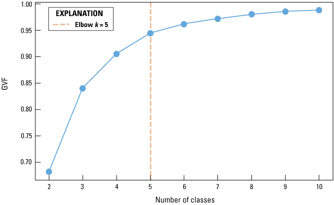
Graph showing Jenks goodness of variance fit (GVF) versus the number of classes (k), with the optimal number of classes identified at the elbow point (k = 5).
-
• The Jenks natural breaks optimization method was applied to the optimal number of classes, which was k = 5.
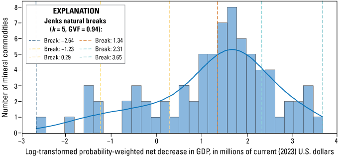
Graph showing the Jenks natural breaks optimization method applied to log-transformed values of probability-weighted net decreases in gross domestic product (GDP) in millions of U.S. dollars. Histogram bars represent the distribution of the number of mineral commodities for given observed log-transformed values. The blue curve overlying the histogram data is a kernel density estimate to more clearly visualize the shape of the distribution. Vertical lines indicate the optimized breakpoints. GVF, goodness of variance fit; k, number of classes.
-
• The resulting class boundaries were transformed back for interpretability in the original scale (millions of U.S. dollars), with cutoff intervals at 0.00 to 0.06, 0.06 to 1.97, 1.97 to 21.97, 21.97 to 205.76, and 205.76 to 4,497.89, which were used to determine the risk categories.
All computations were performed using reproducible Python code, with graphical output illustrating both the GVF curve and final classification breaks.
References Cited
Satopaa, V., Albrecht, J., Irwin, D., and Raghavan, B., 2011, Finding a “Kneedle” in a haystack—Detecting knee points in system behavior, in 2011 31st International Conference on Distributed Computing Systems Workshops, Minneapolis, Minn. June 20–24, 2011: Institute of Electrical and Electronics Engineers, p. 166–171.
Abbreviations
BEA
U.S. Bureau of Economic Analysis
GDP
gross domestic product
HTS
Harmonized Tariff Schedule of the United States
IO
input-output
LCM
List of Critical Minerals
MOFCOM
Ministry of Commerce of the People’s Republic of China
NAICS
North American Industry Classification System
NAPCS
North American Product Classification System
SPOF
single point of failure
USGS
U.S. Geological Survey
Disclaimers
Any use of trade, firm, or product names is for descriptive purposes only and does not imply endorsement by the U.S. Government.
Although this information product, for the most part, is in the public domain, it also may contain copyrighted materials as noted in the text. Permission to reproduce copyrighted items must be secured from the copyright owner.
Suggested Citation
Nassar, N.T., Pineault, D., Allen, S.M., McCaffrey, D.M., Padilla, A.J., Brainard, J.L., Bayani, M., Shojaeddini, E., Ryter, J.W., Lincoln, S., and Alonso, E., 2025, Methodology and technical input for the 2025 U.S. List of Critical Minerals— Assessing the potential effects of mineral commodity supply chain disruptions on the U.S. economy (ver. 2.0, 2026): U.S. Geological Survey Open-File Report 2025–1047, 215 p., https://doi.org/10.3133/ofr20251047.
ISSN: 2331-1258 (online)
| Publication type | Report |
|---|---|
| Publication Subtype | USGS Numbered Series |
| Title | Methodology and technical input for the 2025 U.S. List of Critical Minerals—Assessing the potential effects of mineral commodity supply chain disruptions on the U.S. economy |
| Series title | Open-File Report |
| Series number | 2025-1047 |
| DOI | 10.3133/ofr20251047 |
| Edition | Version 1.0: August 2025; Version 2.0: April 2026 |
| Publication Date | August 25, 2025 |
| Year Published | 2025 |
| Language | English |
| Publisher | U.S. Geological Survey |
| Publisher location | Reston, VA |
| Contributing office(s) | National Minerals Information Center |
| Description | Report: vi, 215 p.; Data Release |
| Online Only (Y/N) | Y |
| Additional Online Files (Y/N) | N |