

Development of a Two-Stage Lifecycle Model to Inform the Trap-and-Haul Program for Oncorhynchus kisutch (Coho Salmon) in the Lewis River, Washington
Links
- Document: Report (5.95 MB pdf) , HTML , XML
- Superseded Publications:
- Download citation as: RIS | Dublin Core
Acknowledgements
We would like to thank Chris Karchesky with PacifiCorp for assistance in data preparation and the reporting of model output. We would also like to thank Kale Bentley with the Washington Department of Fish and Wildlife for his insightful input on model formulation. This study was funded by PacifiCorp and uses data provided by the organization. These data have limited availability. Contact PacifiCorp for more information.
Abstract
Restoration of salmon populations in the upper Lewis River Basin, Washington, depends on a trap-and-haul program owing to the Lewis River Hydroelectric Project (hereinafter referred to as “Project”) operated by PacifiCorp and Cowlitz Public Utilities District (hereinafter referred to as “Utilities”), which has been a barrier to salmon passage since the 1930s. Thus, sustaining the Oncorhynchus kisutch (Walbaum, 1792; coho salmon) population upstream from the Project currently depends on two fundamental factors: (1) the collection of upstream migrating adult coho salmon at Merwin Dam, the lowermost dam within the Project, and transporting them by truck to spawn above Swift Dam, the uppermost dam within the Project; and (2) the collection of out-migrating juvenile coho salmon at the downstream collection facility at Swift Dam for transport and release below the Project. The reintroduction program began once the downstream collection facility at Swift Dam was commissioned in late 2012, with the first year of transport data being collected in 2013. Over the past decade, the Utilities have been collecting data on juvenile outmigrants and adult fish returns at the dams. The need to construct a lifecycle model for Lewis River anadromous fish was identified by the Lewis River Aquatic Technical Subgroup, with the understanding that many years (more than 15 years) of data collection are needed to adequately measure the lifecycle production of salmon. The U.S. Geological Survey was contracted to develop and apply the model to past data at the Lewis River dams to help inform future data collection and provide a framework that can be updated annually to measure trap-and-haul program performance within a lifecycle context.
Because coho salmon can live as long as 5 years, estimating demographic parameters for coho salmon populations over their lifecycle requires at least 10 or more years of data collection. Over the past decade, PacifiCorp has been collecting data on fish collection efficiency and the numbers of adult and juvenile salmon transported around the Lewis River dams, making this an ideal time to formulate a lifecycle model that can guide future data collection efforts and provide preliminary information to resource managers. The goal of the statistical lifecycle model is to estimate annual production and survival during two critical life-stage transitions: (1) the freshwater production from escapement of adults released upstream from Swift Dam, and the collection of downstream migrating juveniles at the downstream passage facility at Swift Dam; and (2) the smolt-to-adult survival from the time of collection at Swift Dam to their return as adults. We used the Beverton-Holt stock-recruitment model to estimate juvenile production from the number of spawners (Beverton and Holt, 1957). This approach allowed us to test for density dependence at current spawner abundances while estimating annual productivity, defined as the number of juveniles produced per spawner at low spawner abundance. Productivity was then expressed as a function of the number of juveniles collected and transported downstream from the Project. Because juvenile fish collection efficiency (FCE) directly affects the number of juveniles that survive to continue downstream migration, FCE is a primary determinant of fish production. Consequently, the modeling framework is well suited to evaluate the performance of trap-and-haul programs within a lifecycle context.
The objectives of this study were to (1) gather and collate available data on adult and juvenile coho salmon at Merwin and Swift Dams; (2) quantify adult escapement, juvenile abundance, and the age at outmigration and adult return; (3) describe, formulate and fit the integrated population model to the data; and (4) summarize our findings, identify data gaps, and identify opportunities for future studies that could improve model estimation and inference. Our key findings were: (1) over and above the number of spawning females, FCE was the primary factor affecting productivity of coho salmon above Swift Dam; (2) smolt-to-adult return (SAR) rates were relatively high considering that harvest was included in the estimate, averaging about 4.5 percent and ranging as high as 12.9 percent; and (3) juvenile capacity upstream from Swift Dam was difficult to estimate due to the limited range in spawning females over the time series of data, suggesting the model may be improved by collecting data at higher spawner abundances. In addition, by including FCE in the model, we estimated that the median pre-collection productivity, defined as the number of juveniles produced per spawner when FCE=1, was 64 juveniles per spawner. Because the two-stage lifecycle model partitions factors that affect fish production in rivers versus the ocean, the model estimates may help inform fishery managers about the overall role that fish collection at Swift Dam plays in the recovery and sustainability of Lewis River coho salmon. By providing the model with (1) more years of data, (2) higher numbers of spawning females, and (3) data on age at juvenile migration in relation to age at adult return, greater certainty in the estimates of capacity and SAR can be attained. Ultimately, information provided by the model may assist in the evaluation and continued improvement of the current trap-and-haul program to support anadromous fishes in the Lewis River Basin.
Introduction
In this report, we present a two-stage state-space lifecycle model (or integrated population model [IPM]) for Oncorhynchus kisutch (Walbaum, 1792; coho salmon) in the Lewis River, Washington (fig 1). The IPM is intended to complement existing spreadsheet-based deterministic lifecycle models often used by fisheries managers to track demographic parameters and determine appropriate hatchery production. In contrast to the deterministic spreadsheet model, the IPM approach incorporates observation and process error in abundance and production estimates (Gelman and others, 2004), allowing users to estimate mean and annual lifecycle demographic parameters and associated uncertainty. Our approach is an extension of the single-stage state-space framework first developed by Fleischman and others (2013) and applied by Courter and others (2019) to Clackamas River O. mykiss (Walbaum, 1792; steelhead), representing a variation of the two-stage state-space model applied to coho salmon in the Cowlitz River Basin, Washington (Plumb and Perry, 2020). Here, the state-space model developed by the U.S. Geological Survey applied to data collected by PacifiCorp consists of two parts: (1) a process model for the underlying state dynamics, and (2) an observation model that links the data to the true underlying state. The state-space model may also be thought of as a hierarchical model where the state (abundance of fish) evolves according to a dynamic population process, such as a Ricker (1954) or Beverton and Holt (1957) model with some process error, and observations on the state (“the data”) are made conditional on the true but unobservable state.
The modeling approach first breaks the lifecycle into juvenile and adult life stages, and then includes population composition, which comprises sex (hatchery or naturally produced), rearing origin, and juvenile and adult-age structure. Multistage lifecycle models provide a powerful analytical framework for understanding how each life stage of a population contributes to population growth rate (Moussalli and Hilborn, 1986; Greene and Beechie, 2004). Multistage models may also be used as an analytical framework to explicitly estimate demographic parameters of a population model. This approach has an advantage over single-stage stock-recruitment models by allowing population growth rates to be partitioned among life stages rather than aggregated over an entire lifecycle. Partitioning among life stages facilitates estimation of (1) stage-specific density dependence, and (2) stage-specific effects of environmental factors or management actions. For example, Zabel and others (2006) estimated parameters of a multistage model used in the context of a population viability analysis for spring and summer O. tshawytscha (Walbaum in Artedi, 1792; Chinook salmon) in the Snake River.
Typically, data informing estimates of abundance at particular “checkpoints” in the lifecycle determine the complexity of the multistage model that can be fit to the data. For coho salmon in the Lewis River Basin, we have developed a two-stage model that encompasses (1) upstream passage of spawners at Merwin Dam to the subsequent downstream passage of their progeny at Swift Dam, and (2) downstream collection of juveniles at Swift Dam to their subsequent return from the ocean and passage at Merwin Dam 1‒3 years later. This approach partitions the lifecycle of coho salmon spatially and temporally, which allows us to fit and compare alternative models with covariates specific to each stage. This report describes the structure of the two-stage lifecycle model as applied to Lewis River coho salmon, presents preliminary results from fitting the model to data, and outlines future directions and developments.
Study Area
The Lewis River Hydroelectric Project (hereinafter referred to as “Project”) begins approximately 16 kilometers (km) east of Woodland, Washington (fig. 1), and consists of 4 impoundments. The sequence of the four Lewis River impoundments upstream from the confluence of the Lewis and Columbia Rivers is as follows: Lake Merwin, Yale Lake, and Swift Reservoir, which includes Swift No. 1 and Swift No. 2 impoundments. Currently, reintroduction efforts for anadromous salmonids are occurring in habitats upstream from Swift Dam. The target species identified for reintroduction are spring Chinook salmon, coho salmon, and winter steelhead. As part of this program, adult salmonids are collected at Merwin Dam and then transported by truck and released into Swift Reservoir to continue their migration to the upper watershed of the Lewis River. When juvenile salmonids migrate downstream, they are collected at the collection facility at Swift Dam, referred to as the Swift Dam floating surface collector (FSC), located at the downstream extent of Swift Reservoir. From there, the juveniles are transported by truck to below Merwin Dam and released at the Woodland Release Ponds before volitionally reentering the Lewis River to continue their downstream migration (fig. 1). Because there is no fish passage currently at Yale or Merwin Dams, juvenile fish that pass Swift Dam into Yale Lake are currently considered lost to the anadromous population.
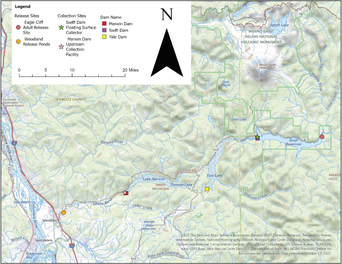
Map of the Lewis River Hydroelectric Project, Washington, showing dams, reservoirs, and locations important to the trap-and-haul program for salmonids.
Methods
Lifecycle models can range from very simple, theoretically based population models (for example, the Beverton-Holt or Ricker stock-recruitment models) to very complex spatially explicit simulation models linked to hydrosystem hydrodynamic models (for example, the COMPASS model for a single transition in a lifecycle model; Zabel and others, 2008). We chose to develop a model of intermediate complexity that casts the two-stage lifecycle model in a state-space framework (Newman and others, 2014). We chose to use a state-space framework implemented in a Bayesian context for the following reasons:
-
• The model provides a statistical estimation framework for retrospective statistical analysis and a stochastic simulation framework for prospective analysis to evaluate alternative management actions.
-
• The model accounts for uncertainty in abundance estimates. A state-space framework accounts for observation uncertainty in the abundance estimates and other data (for example, age structure) while simultaneously estimating process uncertainty.
-
• The model allows for missing data. By drawing missing data from an appropriate probability model, uncertainty owing to missing data can be propagated without having to omit data or assume fixed values for missing data.
Thus, a two-stage state-space lifecycle model for coho salmon strikes an appropriate balance between model complexity, tractability, and applicability given the goals of performing retrospective and prospective analyses to guide future management.
Lifecycle Structure of Lewis River Basin Coho Salmon
The state-space model consists of two parts: (1) a process model for the underlying state dynamics, and (2) an observation model that links the data to the true underlying state. The state-space model may also be thought of as a hierarchical model where the state (abundance) evolves according to a process model for population dynamics (for example, a Beverton-Holt model) with some process error, and observations on the state (“the data”) are made conditional on the true but unobservable state.
First, to model the adult-to-juvenile transition (fig. 2), we used the Beverton-Holt model as opposed to the Ricker model to express the number of juveniles collected at Swift Dam as a density-dependent function of the number of female adults passing Swift Dam in brood year y (PacifiCorp, 2024; Ricker, 1954; Beverton and Holt, 1957):
whereRJ,y
is the true but unobserved number of collected juvenile recruits produced by female spawners,
EF,y
female adult escapement in brood year y,
α
is the productivity parameter estimating the slope at the origin (juvenile recruits per female spawner at low spawner abundance in the absence of density dependence), and
K
is carrying capacity of juvenile recruits and is defined as the maximum number of juveniles that can be produced upstream from Swift Dam.
The process error term, εP,J,y, quantifies annual variation in productivity driven by environmental variation with a mean of zero and a standard deviation of σP,J. Because the productivity of juveniles directly depends on the fraction of juvenile coho salmon collected at Swift Dam, we used annual estimates of FCE (PacifiCorp, 2024), which measures fish capture relative to the number of fish that approached the floating fish collector. This provides an index of fish facility performance from year to year. We modeled the productivity parameter α as a function of the annual FCE and other covariates for coho salmon in the following manner:
whereexp(θ0)
is the mean productivity at the mean covariate value,
θi
is the slope for the effect of the ith covariate on annual productivity, and
xi,y+h
is the ith covariate with an offset of h years on brood year to reflect the life stage in which the covariate is hypothesized to most affect productivity.
The proportion of early spawning coho salmon was defined as those adult coho salmon that arrive at Merwin Dam and are transported during the early (September) compared to the late (October) part of the spawning migration. Note that because the stock-recruitment model was informed by just 10 years of data, we did not fit the model using all covariates on productivity simultaneously. We instead used a stepwise approach where x2−x5 were respectively used to estimate θ2−θ5 within separate models that also included the effect of FCE with θ1x1,y+2. Specifically, x2,y+0 was the data vector for the proportion of hatchery-origin female spawners, x3,y+0 was the proportion of early spawners (Ep), and x4,y+0 was the maximum monthly winter flow indexed to brood year y. The minimum summer flows, x5,y+2, were indexed to the yearling outmigration in year y + 2. Flow data were obtained from the U.S. Geological Survey monitoring site (site identification number 14216500) on the Muddy River located at the upper end of Swift Reservoir (U.S. Geological Survey, 2023). Importantly, when drawing inferences about the effect of FCE on productivity or SAR, we used the model that only included the effect of FCE on productivity in the model. Although the model’s framework is designed to accommodate covariates associated with oceanic effects on SAR, we refrained from adding covariates on SAR at this time because of the lack of information linking juvenile at outmigration to adult age at return to Merwin Dam.
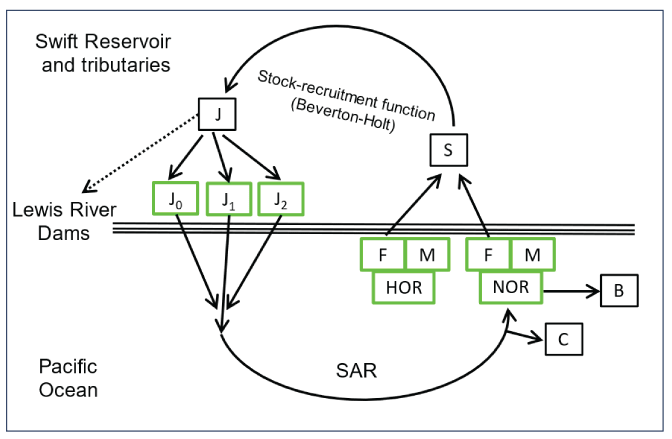
Diagram showing the current structure of the two-stage lifecycle model for Lewis River Oncorhynchus kisutch (Walbaum, 1792; coho salmon), showing juvenile (J) age structure at Swift Dam, Washington (J0, subyearling; J1, yearling; J2, 2-year-old outmigrants), and sex (F, female; M, male) and origin (HOR, hatchery; NOR, natural) of spawning adults (S), while accounting for harvest (C) and brood stock removal (B). The spawner-to-juvenile transition is modeled using a stock-recruitment function, and the juvenile-to-adult transition is modeled with a smolt-to-adult return rate (SAR). Solid arrows designate the structure that is currently incorporated into the model. The dashed arrows designate an unknown quantity of fish that passed downstream from Swift Dam and were lost to the anadromous population. Note that the age structure of returning females and males is only partially known from the jack return of males and, therefore, is not shown.
For the juvenile-to-adult transition, we model the number of adult returns as a lognormal function of a density independent smolt-to-adult return rate (SAR):
whereRA,y
is the number of adult recruits (male and female) produced from the RJ,y juveniles collected at Swift Dam that arose from female spawners in brood year y, and
εP,A,y
is a normally distributed process error with mean of zero and standard deviation of σP,A.
Given that juveniles can pass Swift Dam at ages 0–2 and adults return at ages 1–3, the initial 2 years of juvenile recruits and 3 years of adult recruits that produced returns beginning in 2013 were not linked to the two-stage stock-recruitment model. These initial state vectors were estimated as draws from common lognormal distributions with parameters ln(RJ,0), σRJ0 and ln(RA,0), σRA0, respectively, for juveniles and adults.
Given juvenile recruits, the number of juveniles aJ passing Swift Dam in calendar year t was modeled as the following:
whereis the number of juveniles in year t of age aJ, and
is the proportion of juvenile recruits from brood year y = t – aJ emigrating at age aJ (fig. 3).
Given adult recruits, we model the number of adults returning at age aA of sex s and outmigration strategy o as the following:
whereis the number of adults returning in year t at age aA, of sex s and outmigration strategy o; and
is the proportion of the recruits from brood year y = t – aA returning at age aA, of sex s and outmigration strategy o (fig. 3).
Outmigration strategy refers to whether juveniles were collected at Swift Dam as subyearlings, yearlings, or 2-year-old outmigrants. Because data on the age structure of returning adults for a given age at juvenile outmigration are absent, our current formulation of the two-state model does not account for juvenile age at outmigration in the adult returns, but in the future such information would allow us to estimate SAR separately for each outmigration strategy. Nonetheless, given three adult ocean-age classes (MacLellan and Gillespie, 2015; fig. 3) and three outmigration strategies, the brood-year-specific return probabilities are .
Hypothetical data to reconstruct age-specific juvenile abundance (RJ) and ocean-age-specific adult returns (RA) conditional on juvenile age at outmigration from juveniles (J) generated by spawners (S) in brood year y. Colors represent different brood year classes.
We model the brood-year composition using this structure applied to empirical data on coho salmon in the Lewis River for several reasons. First, juvenile recruitment is expressed as a function of female escapement, requiring estimation of sex structure. Second, age 0–2 juvenile proportions are of direct interest. Third, jack and adult abundances have been recorded since 2012, whereas comprehensive age-structure data have not yet been collected. Thus, using the jack and adult abundance data requires estimating the proportion of jacks in the brood-year return.
Vectors of brood-year-specific marginal and conditional probabilities were modeled hierarchically as draws from a Dirichlet distribution (Fleischman and others, 2013; Scheuerell and others, 2021):
whereis the vector of mean proportions in each age, sex, and age at ocean entry category and is an inverse variance parameter.
Given age-specific juvenile emigration and adult returns from brood year y in calendar year t, the total number of juveniles passing Swift Dam in calendar year t is the sum of the abundance-at-age over all ages:
Note that the current model for coho salmon at Swift Dam accounts for brood stock removal but does not account for juvenile age at outmigration or harvest rates; however, we show here how these estimates can be incorporated into the current framework of the model for future applications. For example, the total number of returning adults in year t is the sum of the abundances across all age, sex, and outmigration classes:Returns of subclasses in year t are calculated similarly by summing over the appropriate indices. For example, the number of female returns in year t is
In addition, the age, sex, and outmigration structure in the adult returns each calendar year is whereis the fraction of the adults returning in year t at age aA, sex s, and outmigration strategy o (in other words, if data on outmigration strategy were included in the model).
Escapement (Et) of spawners past Swift Dam in calendar year t includes hatchery-origin adults released upstream from Swift Dam to spawn in the wild (Ht) plus naturally produced spawners (Nt). The model can accommodate those naturally produced spawners that survive harvest (Ct) or those taken for hatchery brood stock (Bt):
Where the annual harvest rate below Swift Dam can be a composite of ocean harvest that is assumed constant across ages and sexes of returns each year, such that catch is:
whereEscapement of female spawners, which dictates juvenile recruits, is shown in equation 13:
wherefF,t
is the fraction of hatchery-origin adults that are female, and
qF,t
is the proportion of females in naturally produced returns, calculated using equation 14:
The Observation Models
Observations to inform the parameters of the state model include the following:
-
• catch of age-0, age-1, and age-2 outmigrants collected annually at the Swift FSC from 2013–23;
-
• census counts of annual abundance of hatchery-origin and naturally produced adults released above Swift Dam for 2013–23;
-
• estimates of annual run composition of hatchery and naturally produced adults in terms of jacks, adults, and sex for 2013–23;
-
• estimates of the annual number of naturally produced adults removed for hatchery brood stock for 2013–23; and
-
• estimates of ocean harvest rate indices as well as harvest above Swift Dam for 2013–23 (not yet included in the model).
Juvenile Abundance
Estimates of abundance of naturally produced juvenile coho salmon collected at Swift Dam were assumed equivalent to (~) a lognormal distribution about the true abundance:
whereĴt
is the total abundance estimate that includes age-0, age-1, and age-2 fish collected at Swift Dam in year t;
Jt
is the true but latent state vector of juvenile abundances; and
is the observation error.
The observation model for juvenile age composition was done by expressing the juvenile abundance estimates for age 0, age 1, and age 2 as a multinomial distribution:
whereAdult Abundance
The census counts for adult escapement upstream from Swift Dam were assumed to be lognormally distributed with a known coefficient of variation (CV=0.01) calculated as , following Fleischman and others (2013):
whereÊt
is the total escapement for jacks, males, and females released upstream from Swift Dam in year t;
Et
is the true but latent state vector of adult escapement; and
σE
is the observation error.
In the observation model for adult-age composition, census counts of jacks, older males, and females were expressed as a multinomial distribution:
whereParameter Estimation
All parameters and unknown states were estimated in a Bayesian framework using JAGS software (Plummer, 2009) as implemented through the ‘runjags’ package of the R statistical programming platform (R Core Team, 2023). JAGS is a Bayesian estimation software package that implements Markov chain Monte Carlo (MCMC) sampling using a Gibbs or Metropolis-Hastings sampler. Prior distributions for most parameters were set according to Fleischman and others (2013). However, a preliminary model using a weakly informed prior distribution indicated that the data were insufficient to estimate capacity. Therefore, we used information from a meta-analysis on coho salmon populations throughout the Pacific Northwest region to inform the prior distribution on capacity (Korman and Tompkins, 2014). We compare posterior distributions when using the weakly informed versus the informed prior distribution. We used the lognormal distribution parameters provided by Korman and Tompkins (2014) with a mean of 7.46 and standard deviation (SD) equal to 0.67 as the informed prior distribution on capacity. For the weakly informed prior, we used a truncated normal distribution with a μ of 10,000 and an SD of 1,000,000. Comparison of posterior distributions resulting from different prior distributions should help provide a range in capacity estimates for the estimated habitat upstream from Swift Dam. Importantly, the Korman and Tompkins (2014) estimates of capacity were provided on a per-kilometer basis. Therefore, we used 186.9 km of habitat upstream from Swift Reservoir and an additional 14.5 km for the reservoir, resulting in a total of 201.4 km of habitat for salmon. This assumes similar habitat carrying capacity between the reservoir and riverine habitats upstream from Swift Dam.
We ran 3 independent MCMC chains each for 80,000 iterations, discarding the first 30,000 to ensure each chain had converged to its stationary stable distribution. We then thinned the final 50,000 iterations to 1 in 50 to reduce autocorrelation, yielding a final sample of 1,000 draws from each chain. Convergence of each parameter was checked visually to ensure mixing of the chains, and quantitatively by ensuring that the Rubin-Gelman statistic () was less than 1.1 (Gelman and others, 2004).
Estimation of Abundance of Juvenile Coho Salmon Collected at Swift Dam
To implement the two-stage lifecycle model, we first had to estimate the abundance of juveniles collected at Swift Dam. Of the total fish collected, a varying fraction of fish is sampled to determine size and age composition. Although 100 percent of the fish are sampled on most days, on infrequent days during high fish passage, sample rates are lowered for logistical reasons. Over the time series, daily sample rates were as low as 0.1, but 87 percent of the time, sample rates=1. We used the daily sample rates in year t (rd,t) and the counts of juvenile salmon in the sample tank at Swift Dam (cd,t), to estimate the age-specific (a) total abundance of juveniles collected (Jd,t) at the dam.
Estimating age-specific abundance requires classifying juveniles by age (0, 1, and 2). Catch-at-age was determined by PacifiCorp personnel, and we assumed no classification error in age assignment (fig. 4). Daily counts of age-0 fish were considered a complete census, without classification error, owing to their small size at date. Thus, estimation of the total number of age-0 fish (J0d,t) involved simply inflating sample-tank counts by the sample rate, if counts (c0d,t) were binomially distributed:
and for age-1, and age-2 fish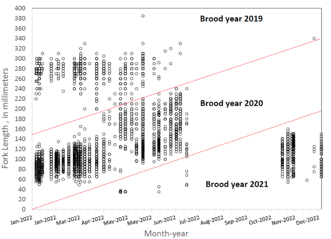
Scatterplot showing an example of age assignment to brood year by fish size and month for juvenile Oncorhynchus kisutch (Walbaum, 1792; coho salmon) collected at Swift Dam, Washington, during 2022.
However, protocols for age assignment of older fish varied across years. In years prior to 2017, age-1 or age-2 was assigned based on size thresholds for subsampled groups (g) whose lengths were measured. The subsampled groups of the collected fish were pooled over 1–6-month periods depending on the year. Because age assignments were based on a measured subsample, we accounted for this sampling error by first estimating age fractions from the subsample and then applying these fractions to the total catch of fish in the sample tank. First, the total number of age-1 and age-2 fish subsampled for a group (sg,t) and the number of age-1 fish (n1g,t) were used to estimate the fraction of age-1 fish (p1g,t):
Given that day d,t fell within the period encompassed by group g,t the daily abundance of age-1 juvenile coho salmon was calculated using the following:
By subtraction, the abundance of age-2 juvenile coho salmon was calculated using the following:Thus, we assume a constant age fraction over each subsample period. The total annual abundance for each age at outmigration (o) was then obtained by adding the Jo,d,t over the total number of sample and fish collection days in calendar year t (Dt):
Results
Summary of Data Used in the Lifecycle Model
The total escapement of coho salmon upstream from Swift Dam was variable but increased slightly over time with the lowest escapement recorded in 2015 (3,754 fish) and the highest escapement in 2020 (9,486 fish; fig. 5). The annual escapement of hatchery-origin fish averaged 5,417 (SD=1,486) with the highest number and fraction of hatchery fish escaping in 2014, whereas natural-origin escapement increased steadily over the time series (fig. 6). In 2013, just 28 naturally produced adult coho salmon were transported upstream from Swift Dam and by 2020, 4,863 natural-origin adults were transported. The fraction of hatchery-origin female spawners (pHOS) generally decreased over time, but pHOS was highly variable, averaging 0.75 (SD=0.182) over the time series. Values of pHOS ranged from a high of 0.99 in 2013 to a low of 0.48 in 2017 and 2020 (fig. 7). The fraction of early spawning coho salmon transported upstream from Swift Dam (Ep) was 1.0 during 2013 and 2014, sharply dropping to 0.08 in 2015, and then showing an increasing trend with Ep=0.8 in 2023 (fig. 8).

Time series of total and female escapement for Lewis River Basin Oncorhynchus kisutch (Walbaum, 1792; coho salmon) upstream from Swift Dam, Washington, 2013–23.
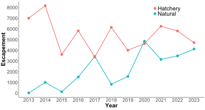
Time series of hatchery and natural-origin escapement for Lewis River Basin Oncorhynchus kisutch (Walbaum, 1792; coho salmon) upstream from Swift Dam, Washington, 2013–23.
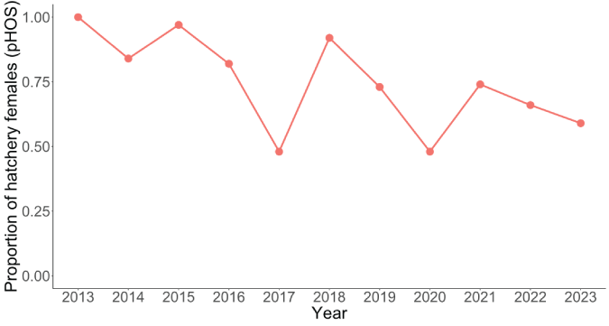
Time series of the proportion of hatchery-origin females out of the total female Oncorhynchus kisutch (Walbaum, 1792; coho salmon) spawning upstream from Swift Dam, in the Lewis River Basin, Washington, 2013–23.
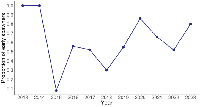
Time series of the proportion of early spawning females out of the total Oncorhynchus kisutch (Walbaum, 1792; coho salmon) spawning upstream from Swift Dam, in the Lewis River Basin, Washington, 2013–23.
The number of natural-origin juvenile coho salmon collected at the Swift FSC (from hatchery and natural-origin spawners) showed an increasing trend over time (fig. 9). Over the annual time series, the average number of juvenile coho salmon collected at the Swift FSC was 50,896 fish (SD±30,771) and ranged from 9,201 fish (SD±46) in 2014 to 100,137 fish (SD±766) in 2019.
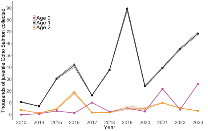
Time series of Lewis River juvenile Oncorhynchus kisutch (Walbaum, 1792; coho salmon) by age at outmigration collected annually at the Swift floating surface collector, in the Lewis River Basin, Washington, 2013–23. The shaded area represents the 5th and 95th credible limits.
Calculation of the proportion of juveniles transported by age at outmigration showed that over the entire time series, age-1 juveniles always represented a majority (greater than 0.55) of the fish collected at the Swift FSC each year (fig. 10). However, in some years either age-0 or age-2 fish represented a sizable proportion of the total number of fish transported. For instance, in 2016, age-2 fish represented 30 percent of all fish collected. Similarly, age-0 fish represented 36 percent of all collected juveniles in 2017 and 30 percent in 2021. Thus, even though age-1 fish were predominant in each year, in some years either very young or older fish represented a sizeable proportion of the juveniles collected.
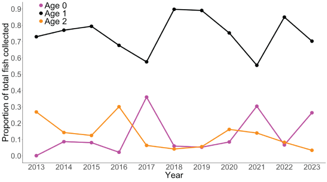
Time series of the proportion of age-0, age-1, and age-2 juvenile Oncorhynchus kisutch (Walbaum, 1792; coho salmon) collected at the Swift floating surface collector, in the Lewis River Basin, Washington, 2013–23.
Fundamentally, the number of juveniles collected at the Swift FSC is determined by the number of spawning females upstream from Swift Dam and the FCE of juveniles at the Swift FSC. Juvenile coho salmon FCE at Swift Dam averaged 0.375 (SD=0.196) and ranged from a low of 0.06 in 2013 to a high of 0.64 in 2019. The time series of FCE suggests an increasing trend in FCE over time (fig. 11). More recent years (2019–23) had higher FCE (mean=0.536, SD=0.129) than years before 2019 (mean=0.242, SD=0.127; fig. 11). These changes in FCE correspond to improvements made to the Swift FSC since it was commissioned in late 2012 (PacifiCorp, 2024). Because the number of spawning adults and juveniles has increased, the number of female spawners and the effect of FCE must be accounted for when estimating lifecycle productivity.
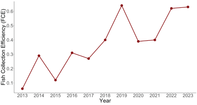
Time series of average annual fish collection efficiency (FCE) at the Swift floating surface collector, in the Lewis River Basin, Washington, 2013–23.
One factor that could also affect the productivity and survival of juvenile coho salmon upstream from Swift Dam is the minimum summer flows during outmigration. Lower summer flows could result in warmer temperatures and physiological stress, higher predator activity, reduced habitat area and thus, lower fish production at Swift Dam. On average, the minimum mean monthly summer flow for our index site on the Muddy River was 149 cubic feet per second (ft3/s; SD=29.4) and ranged from 111 ft3/s in 2015 to 209 ft3/s in 2017 (fig. 12).
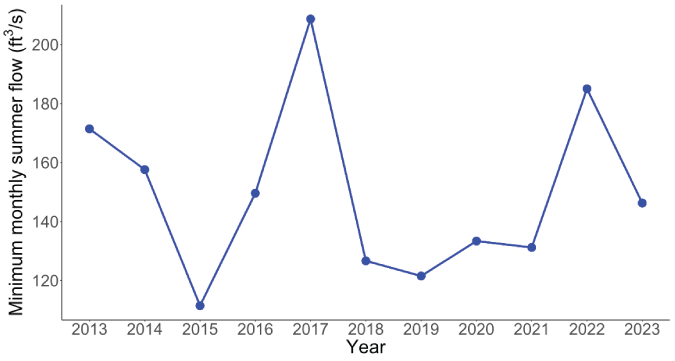
Time series of minimum mean monthly summer (June, July, and August) flow as measured at the Muddy Creek tributary upstream from Swift Reservoir, Washington, 2013–23. Data are from U.S. Geological Survey (2023). [ft3/s, cubic foot per second]
Parameter Estimates Under the State-Space Model
Posterior distributions represent the uncertainty about the model parameters (table 1; figs. 13 and 14). Annual FCE was found to have a strong positive effect on productivity with a median of 1.962 (95-percent credible interval [CI]=0.247–4.079). The fraction of the posterior distribution less than zero was 0.008, indicating that FCE at the Swift FSC had a positive effect on the number of recruits per spawner that contribute to the population. The median of the posterior for mean productivity across years when FCE=1 was αFCE=1=64 naturally produced juvenile recruits per female spawner (95-percent CI=10.37–245.79; table 1.1; fig. 14). Assuming a mean fecundity of 2,600 eggs (Beacham, 1982) per female, this equates to a mean egg-to-juvenile outmigrant survival of about 2.4 percent at low spawner density.
Evaluations of individual effects on productivity over and above the effects of FCE indicated that minimum monthly summer flow had a negative effect on annual productivity (tables 1, 1.1, and 1.2; fig. 13). About 95 percent of the posterior distribution for θ5were less than 0, indicating statistical support for an effect of minimum summer flow on productivity. Also, the fraction of hatchery spawners tended to have a negative effect on productivity, with 80 percent of the posterior distribution having θ2 less than 0. In contrast, a larger fraction of early spawning coho salmon was associated with generally higher juvenile productivity, with 17.5 percent of the posterior distribution having θ3 less than 0. The effect of maximum monthly winter flows on juvenile productivity was not statistically supported with a posterior that encompassed zero, with 34 percent of the posterior less than zero.
Using population level estimates of capacity from Korman and Tompkins (2014) to inform the prior distribution for capacity (K) of Lewis River coho salmon resulted in a well-defined posterior distribution with a median capacity of 297,901 (95-percent CI=84,584–812,488) maximum juveniles produced (table 1; figs. 14 and 15). Uncertainty about the estimate of capacity is demonstrated by how the choice in prior distribution can influence the estimate of capacity. For example, when a weakly informed prior using a truncated normal distribution where K ~ normal(μ=10,000, SD=1,000,000), median capacity was 645,779 (95-percent CI=58,373–1,903,420) juveniles, and the posterior distribution was much more protracted compared to the posterior distribution informed by Korman and Tompkins (2014; fig. 14), K ~ lognormal(μ=7.34, SD=0.67). Nonetheless, the posterior distributions were similar to their respective prior distributions, supporting the conclusion that the data provided little information towards the estimation of capacity in the lifecycle model.
Table 1.
Summary statistics for posterior distributions for the two-stage lifecycle model of Lewis River Oncorhynchus kisutch (Walbaum, 1792; coho salmon) showing parameters for the Beverton-Holt model, smolt-to-adult return rate, observation, and process error, as well as the autocorrelation coefficients, in the Lewis River Basin, Washington.[Also shown is the estimated mean productivity when fish collection efficiency (FCE)=1 and capacity (K) as estimated using an informed and weakly informed prior distribution. Notice that all estimates are provided while estimating the effects (θ0−5) of FCE on juvenile productivity is included in the model. Abbreviations: %, percent; CI, credible interval; SD, standard deviation; pHOS, fraction of hatchery-origin female spawners; max, maximum; min, minimum]
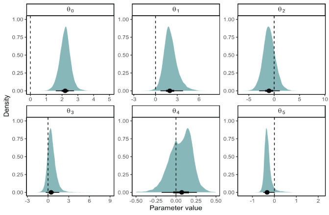
Posterior distributions for the intercept θ0and the effect of fish collection efficiency (θ1) on productivity, the effect of the fraction of hatchery female spawners (θ2) and early spawners (θ3), and effects of the maximum monthly winter flow (θ4) and minimum monthly summer flow (θ5) under the Beverton-Holt stock-recruitment model for Lewis River Oncorhynchus kisutch (Walbaum, 1792; coho salmon) in the Lewis River Basin, Washington. Posterior summaries at the bottom of each panel show the median (circle), 90-percent credible interval (thin line), and 50-percent credible interval (thick line). Vertical dashed line denotes 0.
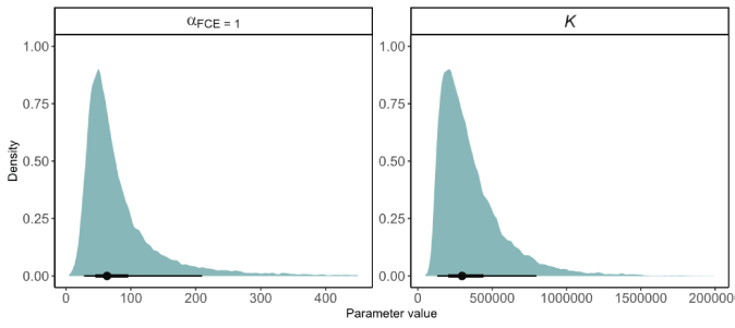
Posterior distributions of productivity estimated when fish collection efficiency (FCE)=1 and carrying capacity (K) as estimated under the Beverton-Holt stock-recruitment model for Lewis Oncorhynchus kisutch (Walbaum, 1792; coho salmon), in the Lewis River Basin, Washington. A prior distribution with parameters from Korman and Tompkins (2014) was used to inform the posterior distributions. Posterior summaries at the bottom of each panel show the median (circle), 90-percent credible interval (thin line), and 50-percent credible interval (thick line).
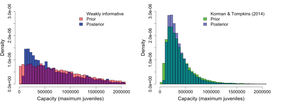
Histograms showing the use of a weakly informed (left panel) or informed (right panel) prior distributions and their resulting posterior distributions for estimating the carrying capacity of Lewis Oncorhynchus kisutch (Walbaum, 1792; coho salmon) upstream from Swift Dam, Washington.
The curves from the Beverton-Holt stock-recruitment model illustrate how recruitment of naturally produced juveniles varies as a function of the number of female spawners (fig. 16). The data used to inform the stock-recruitment model encompassed a relatively narrow range in the number of spawners and juveniles, from a low of 1,074 to about 4,993 female spawners. So, our estimated stock-recruitment model parameters provide inference over a narrow range of observed population levels as supported by the uncertainty in our estimates of capacity (fig. 15).
For the juvenile-to-adult transition, the median of the posterior for the mean SAR across all years was 0.045 (95-percent CI=0.001–0.13; table 1). Thus, in the absence of accounting for harvest, a median of 4.5 percent of juvenile outmigrants returned to the Lewis River. Owing to the hierarchical structure of the state-space model, annual variation in productivity and SAR can be estimated as random effects drawn from the lognormal process error (σP,J and σP,A; table 1.1; figs. 16 and 17). SAR and productivity vary considerably over time and generally increase after brood year 2015. The higher productivity since brood year 2015 coincides with increasing FCE since 2015 (fig. 11). The number of juveniles collected at Swift Dam given the number of female spawners showed the increase in productivity of natural juveniles upstream from Swift Dam because of higher juvenile fish collection performance at the Swift FSC (figs. 16 and 18).
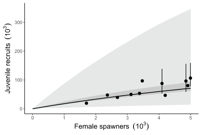
Plot showing the fitted Beverton-Holt function based on posterior medians of parameters expressed as production of juvenile recruits. Note that the stock-recruitment curve was estimated using the mean fish collection efficiency (FCE)=0.375 over the time series. The dark shaded area represents the 95-percent credible interval about the mean trend, and the light shaded area represents the 95-percent credible interval when process error is considered. The error bars represent the point-wise 95-percent credible interval about the estimated juvenile recruits.
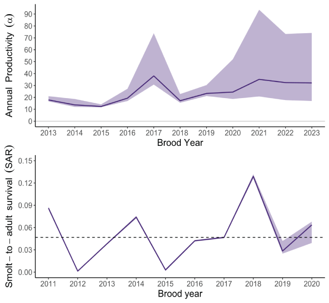
Plots showing annual estimates of juvenile productivity (recruits per spawner; top panel) between brood years 2013 and 2023 and smolt-to-adult return rate (SAR; bottom panel) between brood years 2011 and 2020. Lines connect annual medians of posterior distributions, shaded areas represent the 5th–95th credible interval, and the dashed line shows the overall median for SAR (0.045).

Plot showing the relation between fish collection efficiency (FCE) and the number of juveniles per spawner, shaded area represents the 95-percent credible interval about the mean effect of FCE, and the error bars represent the 95-percent credible interval about the estimated annual productivity. The dashed line represents the extrapolated estimate of productivity when FCE=1 (pre-collection productivity).
Conclusions
The state-space lifecycle model for Lewis River Oncorhynchus kisutch (Walbaum, 1792; coho salmon) in the upper Lewis River Basin, Washington, is a model of intermediate complexity but can be used to gain insight about population dynamics and factors affecting different life stages as part of the ongoing reintroduction program. The state-space formulation of the model accounts for observation and process error, provides estimates of uncertainty in abundance and demographic parameters, and quantifies contributions of age and sex to the aggregate population. Our formulation of the state-space model provides a wealth of information about population dynamics such as estimates of process uncertainty, carrying capacity and density dependence, juvenile-to-adult survival rates, and factors affecting production of juvenile coho salmon upstream from Swift Dam, the latter being particularly important for understanding how fish collection efforts at the Swift floating surface collector (FSC) affect population sustainability and recovery. We also demonstrate how the model can be expanded to include juvenile age at outmigration and subsequent age at return, harvest, as well as ocean effects on demographic parameters such as juvenile-to-adult return rate.
The lifecycle model for Lewis River coho salmon can be used to provide estimates of the effect of fish collection efficiency (FCE) on adult-to-juvenile productivity. This analysis represents an initial effort that illustrates the utility of multistage statistical lifecycle models for understanding the interplay between population dynamics and trap-and-haul programs that seek to sustain salmon populations. There are many other aspects of the dynamics of this population that we have yet to explore. For example, there is much uncertainty in the estimation of capacity under the Beverton-Holt model because of the limited range in escapement and the number of spawning females. Regardless of the uncertainty, our informed estimates of capacity (median=297,901) were much larger than recent juvenile fish collection at the Swift FSC, supporting the conclusion that higher escapement numbers might result in higher juvenile abundance. Therefore, firm conclusions regarding the capacity of habitat for coho salmon upstream from Swift Dam should be withheld at this time. Additional information regarding productivity at higher escapement is needed before a more definitive conclusion can be made. By also incorporating a fuller set of covariates, harvest rates, and juvenile age structure in relation to their age at adult return into the model, parameter estimates may provide a broader set of inferences to the individual contribution of these factors to the lifecycle of coho salmon upstream from Swift Dam.
We estimated the effect of several covariates on juvenile production. Perhaps high flows push fish into the reservoir where they experience a higher predation rate. Thus, even though we found strong statistical support for the negative effects of high flows on juvenile coho salmon productivity, the mechanisms behind such an effect are unclear. For other effects on juvenile productivity, higher fractions of hatchery fish were moderately associated with lower juvenile productivity, with 80 percent of the posterior distribution having θ2 less than 0, suggesting lower juvenile production at higher fractions of hatchery escapement (fig. 13). Higher fractions of early spawning females also were poorly associated with higher juvenile productivity, with 82.5 percent of the posterior distribution having θ3 greater than 0. After including FCE in the model, there was little variation to be explained from 10 data points, and uncertainty in model parameters has much room for improvement, so inferences about model covariates should be made cautiously. Additional years of data may help provide a clearer picture of the factors that affect juvenile production upstream from Swift Dam.
There are several significant updates that could improve model fit and provide greater inference for fishery management. These updates include (1) accounting for ocean harvest rates for naturally produced fish; (2) obtaining data on age at return for each juvenile age at outmigration, allowing for more precise indexing of covariates and the estimation of smolt-to-adult return rate (SAR); and (3) evaluating other covariates to explain variation in adult-to-juvenile productivity (α) and SAR (Logerwell and others, 2003).
Some of the future covariates that could help explain variation in adult-to-juvenile production include using the median date of adult transportation as an alternative measure of spawn timing effects.
Future covariates that may help explain variation in annual smolt-to-adult return rates include the following:
-
• juvenile age at outmigration,
-
• Pacific decadal oscillation,
-
• coastal upwelling index,
-
• sea surface temperatures, and
-
• harvest estimates in the ocean and freshwater downstream from Merwin Dam.
Regardless of the improvements that can be made to the model, we can safely draw some conclusions. First and perhaps foremost, we were able to quantify how FCE at the Swift FSC directly determines the productivity of juveniles. This was demonstrated by the relation between mean annual productivity and FCE. Thus, the annual progression towards higher FCE at the Swift FSC (in other words, since 2013) contributed to the higher productivity and greater numbers of juveniles collected in recent years. However, there is little data at high FCE values (those greater than 0.64) with much uncertainty in juvenile productivity at the upper end of the FCE curve, such as when FCE=1.
Perhaps the model’s most uncertain parameter for the adult-to-juvenile life stage is carrying capacity of the habitat upstream from Swift Dam, K. Over the historical time series, there have not been enough spawners released upstream from Swift Dam to elicit compensation in juvenile fish production. Consequently, there is much uncertainty in our estimation of coho salmon capacity for the habitat upstream from Swift Dam. This uncertainty is evident when comparing the results from using an informed and uninformed prior distribution to estimate capacity. Using the distribution parameters from the meta-analysis of coho salmon capacity provided by the literature as an informed prior distribution yielded a much lower and certain estimate of capacity than using a weakly informed prior, which yielded a much higher and uncertain estimate of capacity than using the informed prior. Both posterior distributions closely followed their respective prior distribution, which suggests the data alone are insufficient for estimating capacity. In preliminary model runs, we compared median capacity with and without the 14.5 kilometers distance of the reservoir, and the difference was trivial when considering the uncertainty in the capacity estimate, with the distance of the reservoir producing an additional 21,447 juveniles. However, including the distance of the reservoir in the calculation in this way assumes that the reservoir and riverine habitats upstream from the reservoir provide the same production and capacity benefits for coho salmon. Future efforts towards releasing a sufficiently high number of adult coho salmon upstream from Swift Dam may help inform our estimate of capacity and when compensation in juvenile production should be expected.
The median SAR over all estimable years of about 4.5 percent is relatively high when one considers that this survival rate includes harvest mortality. Estimates of SAR by brood year ranged from 0.1 percent in 2012 to 12.9 percent in 2018. However, we should be cautious in drawing many inferences from our current estimates of SAR because the model does not yet account for juvenile outmigration and their respective age at return, which can bias age-averaged estimates of SAR. Analysis of scale samples from returning adults with juvenile age at ocean entry and adult age at return could be incorporated into the model to help resolve this uncertainty. Notwithstanding this limitation, our annual estimate of SAR suggests that in some years, return rates may be high enough to meet replacement and sustain the population, as long as juvenile production and fish collection remain at some yet unknown, but sufficiently high value. Future applications of the model could include a population viability analysis to determine what FCE target may be needed to sustain Lewis River coho salmon.
Ultimately, fisheries managers need tools to help understand how potential management actions affect population abundance at different parts of the lifecycle in order to assess whether recovery goals are being achieved. The state-space lifecycle model for Lewis River coho salmon takes a first step towards developing such a tool. Additional work could help better account for key management factors affecting the population (for example, harvest), to quantify the contribution of the trap-and-haul program performance, and to incorporate the effects of environmental variation. Because the model incorporates unaccounted for variability in demographic parameters, we can use the model to simulate stochastic population trajectories that include important factors that might be altered for the purposes of management (for example, FCE and harvest) under expected environmental variation. Such a model could allow managers to assess the relative effect of alternative management scenarios on population trajectories in a probabilistic manner to understand the likelihood of success of a given management action in the face of environmental variability and uncertainty.
References Cited
Korman, J., and Tompkins, A., 2014, Estimating regional distributions of freshwater stock productivity, carrying capacity, and sustainable harvest rates for coho salmon using hierarchical Bayesian modelling: Department of Fisheries and Oceans, Canadian Science Advisory Secretariat research document 2014/089, 53 p.
Newman, K.B., Buckland, S.T., Morgan, B.J.T., King, R., Borchers, D.L., Cole, D.J., Besbeas, P., Gimenez, O., and Thomas, L., 2014, Modeling population dynamics—Model formulation, fitting and assessment using state-space methods: New York, Springer, 215 p. [Also available at https://doi.org/10.1007/978-1-4939-0977-3.]
Plumb, J.M., and R.W. Perry, 2020, Development of a two-stage life cycle model for Oncorhynchus kisutch (coho salmon) in the upper Cowlitz River Basin, Washington: U.S. Geological Survey Open-File Report 2020–1068, 25 p., accessed June 1, 2021 at https://doi.org/10.3133/ofr20201068.
Plummer, M., 2009, Jags version 1.0.3 manual—Technical report: Halifax, Nova Scotia, Canada, Dalhousie University, 47 p. [Also available at https://www2.stat.duke.edu/~rcs46/jags_tutor.pdf.]
R Core Team, 2023, R—A language and environment for statistical computing, version 4.2.1 (runjags): R Foundation for Statistical Computing software release, accessed June 2022, at http://www.r-project.org and https://cran.r-project.org/web/packages/runjags/index.html.
U.S. Geological Survey, 2023, USGS Water Data for the Nation: U.S. Geological Survey National Water Information System database, accessed July 18, 2023, at https://doi.org/10.5066/F7P55KJN.
Zabel, R.W., Faulkner, J., Smith, S.G., Anderson, J.J., Van Holmes, C., Beer, N., Iltis, S., Krinke, J., Fredricks, G., Bellerud, B., Sweet, J., and Giorgi, A., 2008, Comprehensive passage (COMPASS) model—A model of downstream migration and survival of juvenile salmonids through a hydropower system: Hydrobiologia, v. 609, no. 1, p. 289–300.
Appendix 1
Table 1.1.
Summary statistics for posterior distributions of adult-to-juvenile productivity for Oncorhynchus kisutch (Walbaum, 1792) estimated for each brood year.[Abbreviations: %, percent; CI, credible interval; SD, standard deviation]
Table 1.2.
Summary statistics for posterior distributions of smolt-to-adult return rates (SAR) for Oncorhynchus kisutch (Walbaum, 1792) showing parameters for each brood year.[Abbreviations: %, percent; CI, credible interval; SD, standard deviation]
For more information about the research in this report, contact
Director, Western Fisheries Research Center
U.S. Geological Survey
5501-A Cook Underwood Road,
Cook, Washington 98605-9717
Manuscript approved on March 18, 2026
Publishing support provided by the U.S. Geological Survey Science Publishing Network, Baltimore and Tacoma Publishing Service Centers
Disclaimers
Any use of trade, firm, or product names is for descriptive purposes only and does not imply endorsement by the U.S. Government.
Although this information product, for the most part, is in the public domain, it also may contain copyrighted materials as noted in the text. Permission to reproduce copyrighted items must be secured from the copyright owner.
Suggested Citation
Plumb, J.M., and Perry, R.W., 2026, Development of a two-stage lifecycle model to inform the trap-and-haul program for Oncorhynchus kisutch (coho salmon) in the Lewis River, Washington: U.S. Geological Survey Open-File Report 2026–1004, 24 p., https://doi.org/10.3133/ofr20261004. [Supersedes preprint https://doi.org/10.1101/2025.04.30.651546.]
ISSN: 2331-1258 (online)
Study Area
| Publication type | Report |
|---|---|
| Publication Subtype | USGS Numbered Series |
| Title | Development of a two-stage lifecycle model to inform the trap-and-haul program for Oncorhynchus kisutch (coho salmon) in the Lewis River, Washington |
| Series title | Open-File Report |
| Series number | 2026-1004 |
| DOI | 10.3133/ofr20261004 |
| Publication Date | April 22, 2026 |
| Year Published | 2026 |
| Language | English |
| Publisher | U.S. Geological Survey |
| Publisher location | Reston, VA |
| Contributing office(s) | Western Fisheries Research Center |
| Description | vii, 24 p. |
| Country | United States |
| State | Washington |
| Other Geospatial | Lewis River |
| Online Only (Y/N) | Y |
| Additional Online Files (Y/N) | N |