

High-Resolution Magnetic Survey Using an Unoccupied Aerial Vehicle to Constrain Buried Lava Flow Geometry, Volume, and Eruptive History of Little Cones, Crater Flat, Nevada
Links
- Document: Report (5.6 MB pdf) , HTML , XML
- Larger Work: This publication is Chapter R of Distributed volcanism—Characteristics, processes, and hazards
- Data Release: USGS data release - Data and codes utilized for the study of the lava flow of Little Cones, Nevada, USA, using UAV magnetic data (ver. 1)
- NGMDB Index Page: National Geologic Map Database Index Page (html)
- Download citation as: RIS | Dublin Core
Acknowledgments
The authors would like to thank our reviewers Victoria Langenheim and Takao Koyama for their comments and suggestions. We also want to thank the editors and the U.S. Geological Survey for organizing this volume along with the organizers of the American Geophysical Union Chapman Conference where this work was initially presented. Lastly, we would like to thank SENSYS Magnetometers & Survey Solutions for help with the magnetometer. Most color schemes used here are from Crameri (2023), which are color vision deficiency (color-blindness) friendly.
Abstract
Magnetic surveys are an important tool used to augment geologic mapping in distributed volcanic fields. Using magnetic anomalies, it is possible to model the geometry of shallowly buried volcanic features, such as conduits, sills, and lava flows. This subsurface mapping is important for understanding eruption dynamics and emplacement of lava flows, and it sometimes reveals buried volcanoes no longer visible at the surface. These data are critical to better interpret the numbers, styles, and magnitudes of eruptions in distributed volcanic fields and their associated volcanic hazards. New advances in unoccupied aerial vehicles (UAVs) offer an attractive middle range of resolution and aerial coverage between ground-based magnetic surveys and aeromagnetic surveys.
Here, we present the results of a UAV fluxgate magnetic survey of the Little Cones, Nevada, scoria cones, which have been the target of previous ground and aeromagnetic surveys. The magnetic anomalies at Little Cones are of interest because the surrounding alluvium conceals lava flows that erupted from Little Cones, making it very difficult to understand the volume and morphology of lava flows from geologic mapping alone. Nonlinear inversion of UAV-collected magnetic data were used to model the thickness and morphology of buried Little Cones’ lava flows with higher precision than achieved previously. The sequence of events and calculated flow characteristics are then interpreted. The total volume of Little Cones, including concealed lava flows, is approximately 0.016 cubic kilometer, and the initial sheet flow erupted in less than 24 hours. The findings presented herein demonstrate that UAV-based magnetic surveys are a reliable method of data collection and an efficient alternative to other survey methods, facilitating development of a three-dimensional perspective of distributed volcanic fields.
Introduction
Volcano morphology and eruptive products provide insights into the scales of past eruptive events, eruption dynamics, changes in eruptive behavior, and volcanotectonic interactions (for example, Wright and others, 2006; Whelley and others, 2015; Bakowski, 2025). Characterization of these eruptive features is critical for volcanic hazards assessments (Bebbington, 2014; Sheldrake, 2014; Idaho National Laboratory [INL], 2024). For example, the volumes of lava flows are used to estimate eruption rates and how they change with time, as well as to forecast future eruption rates (Bacon, 1982; Kuntz and others, 1986; Valentine and Perry, 2007; Gallant and others, 2018). Volume data coupled with isotopic age determinations can be used to estimate recurrence rates and changes in eruptive volume with time (Kuntz and others, 1986; Fleck and others, 1996; Heizler and others, 1999; Nicholis and Rutherford, 2004; INL, 2024). Determining the eruptive history informs forecasts about future eruptive activity, especially in spatially distributed volcanic fields (Connor and Hill, 1995; Gallant and others, 2018; INL, 2024); however, these volcanic deposits may be obscured in some cases by more recent products, thereby complicating interpretations.
Purpose of Magnetic Survey
Magnetic surveys are highly effective for mapping buried features in basaltic volcanic fields because basalts have high remanent magnetization and magnetic susceptibilities, as documented for the basalt in our study area (Champion and others, 1988; Fleck and others, 1996) and elsewhere (for example, INL, 2024). Shallow volcanic features, such as dikes, sills, and buried lava flows, produce high magnetic gradients and complex anomalies. Magnetic surveys usually must have the following to accurately capture such detail: very high spatial resolution (line spacing <100 meters [m]), high sample density along survey lines (<2 m), and consistent low sensor height (10–40 m above ground level [AGL]). The high fidelity of magnetic inversions achieved is demonstrated herein by using high-resolution data collected by unoccupied aerial vehicles (UAVs). These inversions, which translate magnetic anomalies into geometric models of the subsurface, provide essential details about lava flow volume and morphology.
The survey documented herein is of the Little Cones volcanoes and surrounding alluvium in Crater Flat, Nevada. Crater Flat has been studied extensively to characterize the hazards associated with a distributed volcanic field located near the proposed nuclear waste repository at Yucca Mountain (for example, Carr and Parrish, 1985; Champion, 1991; Connor and Hill, 1995; Langenheim, 1995; Fleck and others, 1996). These studies resolved uncertainties about the number of volcanic features in this region, some of which are completely buried in alluvium, and provided constraints to the risk posed by this volcanism to the proposed waste repository. Of particular interest here, the use of high-resolution magnetic surveys by several of these studies (for example, Connor and others, 1997; Stamatakos and others, 1997; Perry, 2005; Valentine and others, 2006) identified volcanic cones that are not visible at the surface.
The Little Cones are two small-volume scoria cones located in the southern part of Crater Flat (fig. 1), a slowly subsiding basin within which sediment is accumulating, bounded by the Bare Mountain fault and the Yucca Mountain fault zone, eastern and western groups (Stamatakos and others, 1997). Because of post-eruptive sediment accumulation in the basin, nearly the entire lava flow field associated with the Little Cones eruptions is not visible at the surface. Previous magnetic surveys and drilling have been used to identify the buried basaltic lavas of Little Cones as well as other buried lavas and sills in Crater Flat and adjacent basins (Connor and others, 1997; Blakely and others, 2000; La Femina and others, 2002; George and others, 2015).
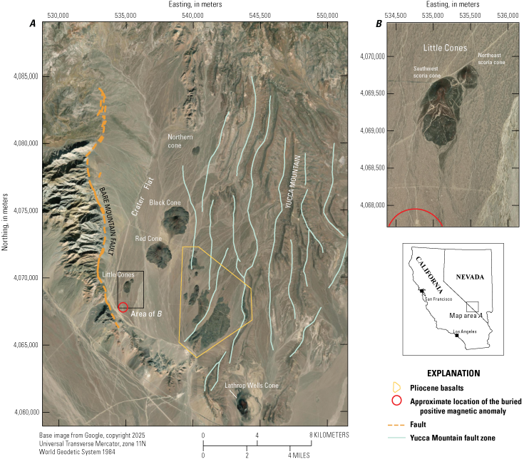
A, Map of Little Cones in southern Crater Flat, Nevada. B, Map of study area extent around Little Cones. Fault line data in A are from U.S. Geological Survey and New Mexico Bureau of Mines and Mineral Resources [2021]. The buried positive magnetic anomaly has been referred to colloquially in the scientific community since 1995 as the “Jerry Garcia anomaly.”
In this study, we used UAVs to collect high-resolution magnetic data that were then inverted to map in great detail the subsurface lava flows associated with Little Cones. The following section provides a brief review of literature on small-volume basaltic volcanism relevant to the interpretation of magnetic anomalies. The field methods used to collect magnetic data and high-resolution digital topography by UAV are then described, including the use of survey lines at multiple altitudes to check survey fidelity. The magnetic data are then modeled using inversion codes written for this purpose, and these lava flow models are used to propose a model of lava flow emplacement and eruption dynamics. By achieving high data density with the UAV survey and by implementing high-resolution inversion, we show that it is possible to deduce the sequence of events and volcanic processes that formed Little Cones, even though these are largely obscured at the surface. Data and codes used in this manuscript are available in Van Alphen and others (2026).
Geology of Scoria Cones, Lava Flows, and their Magnetic Anomalies
Scoria cones and their attendant vents and lava flows are sometimes described as simple volcanic structures, but they evolve through stages of activity, growth, and destruction. The morphology and relation of scoria cones and vents to lava flow fields reveal important details of their eruptive histories (Martin and Németh, 2006; Riggs and Duffield, 2008; Németh and others, 2011; Kereszturi and others, 2012; Courtland and others, 2013; Kiyosugi and others, 2014). These eruptions are often initiated by dike intrusion, leading to fissure eruptions at the surface. As flow localizes along the fissure, Hawaiian- or Strombolian-style cone building begins. The scoria cone consists of layers of scoria, agglutinate, and blocks that are usually emplaced by downslope movements and variable welding, creating complex facies within the cone (Martin and Németh, 2006). Laboratory models (Tibaldi,1995; Németh and others, 2011) indicate that pressure can then increase inside cones, leading to lava breaching of the cone flanks. Breaching then rafts away blocks of the inner and outer flanks and can produce a more violent style of eruption caused by the sudden drop in overpressure (Németh and others, 2011; Kiyosugi and others, 2014). Either the cones heal these breached sections or the eruptive phase ends, leaving a cone with a missing flank section (Tibaldi, 1995). Alternatively, horseshoe shaped cones can form syn-eruptively as spatter material is continuously transported downslope during active lava emission. This process leaves a section of the cone missing where the cone never built up. (Németh and others, 2011; Kereszturi and others, 2012).
These different eruptive processes leave magnetic signatures that can be delineated with very high-resolution magnetic mapping techniques. For example, early, less explosive Strombolian phases and accumulation of ephemeral lava lakes will create relatively coherent and high-amplitude magnetic anomalies because these processes allow basalt bodies to accumulate with coherent vectors of magnetization owing to their high temperature of emplacement (Riggs and Duffield, 2008; Marshall and others, 2015; Özyalın, 2023). Processes from Strombolian or other explosive eruption types lead to relatively high eruption columns and pyroclasts that cool through the Curie point in flight or as they hit the ground, shatter, and roll. Such deposits will have low bulk remanent magnetization and do not produce strong magnetic anomalies (López Loera and others, 2008; Athens and others, 2014). Similarly, rafting of cone walls results in lowering of bulk magnetization of the rafted strata if they break apart. Conversely, if the rafted cone sections remain internally intact but rotate (Sumner, 1998), magnetic anomalies will be produced that are caused by the rotated, remanent component of magnetization. Importantly, these scoria cone and lava flow structures are often tens of meters in scale. Magnetic surveys and inversion modeling algorithms must have comparable resolution to adequately map these features and their associated complexities, thereby providing a view of near-surface and deeper interfaces that can help distinguish geologic structures and the order of eruptive events.
In surface exposures, Little Cones are composed of fragmented pyroclastic material (predominantly unconsolidated scoria) and lava flows that crop out near the cones before being buried in alluvium in their distal parts (fig. 2A; Faulds and others,1994). The lava flows were previously modeled to be 15–20 m beneath the alluvium (Stamatakos and others,1997) and are associated with strong negative magnetic anomalies indicating eruption during the Matuyama reversed polarity chron (Connor and others, 1997; Stamatakos and others, 1997; Blakely and others, 2000). The isotopic age of Little Cones is 1.042 ±0.045 mega annum (Ma) (Faulds and others, 1994), which places it either just before or during the Jaramillo normal polarity sub-chron (Horng and others, 2002), indicating some uncertainty in its age. Regardless, Little Cones are two of several cones in a local sequence of aligned vents consisting of an unnamed northern cone, Black Cone, Red Cone, and Little Cones (fig. 1; Faulds and others, 1994; Heizler and others, 1999). Stamatakos and others (1997) estimated an exposed volume of approximately 0.00063 cubic kilometer (km3) for the southwest scoria cone of Little Cones, approximately 0.00017 km3 for the northeast scoria cone of Little Cones, and more than 0.01 km3, possibly as much as 0.02 km3, for the total volume of the cones and associated lava flows, as mapped by ground magnetic data. Hereafter, the two scoria cones will be referred to individually in generic form as “the southwest scoria cone” and “the northeast scoria cone.”
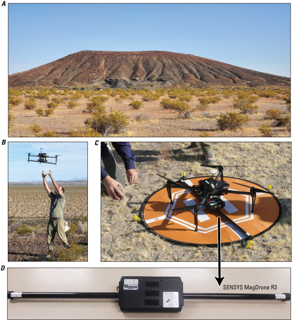
A, Photograph showing the southwest scoria cone of Little Cones looking approximately east. Photograph by Laura Connor taken in 2019, used with permission. B, Photograph showing unoccupied aerial vehicle (UAV) being caught before landing on vegetation. Photograph by Laura Connor taken in 2019, used with permission. C, Photograph showing DJI Matrice 100 UAV with SENSYS Mag Drone R3. Photograph by Laura Connor taken in 2019, used with permission. D, Photograph showing SENSYS Mag Drone R3. Photograph by Robert Van Alphen taken in 2025.
Methods
Field Methods
Magnetic Survey
The magnetic and photogrammetry surveys were conducted during October 17–22, 2019. Because of high-wind conditions and technical problems, data were not collected every day. We used a Sensys MagDrone R3 Fluxgate magnetometer rigidly mounted on a DJI Matrice 100 UAV (fig. 2B–D). The lightweight magnetometer (884 grams) contains two triaxial fluxgate sensors, one at each end of a 1-m-long carbon fiber rod, with the data-logger, Global Navigation Satellite System receiver, and battery pack housed between the two sensors (fig. 2D). The sensor assembly was mounted at the base of the UAV; hence, the magnetic sensors were each located about half a meter away from the center of the UAV (fig. 2C).
The UAV flew 40 m AGL as defined by the 30 m SRTM digital elevation model (DEM) (Farr and others, 2007). This draped survey allowed terrain effects to be accounted for. Survey lines were spaced at 50 m intervals across most of the field site, with an additional set of survey lines spaced 10 m apart above the two scoria cones, where topographic and magnetic gradients are steepest (fig. 3). Both north-south and east-west lines were flown. We downloaded data from the magnetometer between flights and created magnetic maps in the field, thereby allowing flight planning updates in the field to ensure that the full extent of the magnetic anomaly was mapped. Areas of low magnetic signals were avoided, and flights were extended where a strong magnetic signal or gradient was observed. During the 3.5 days of magnetic surveying, over 200 line kilometers (km) of data were collected at 200 hertz (Hz), covering an area 1.7 km x 3 km (fig. 3). A Global Positioning System (GPS) unit embedded in the Sensys MagDrone collected data at 5 Hz and was used to time and locate the magnetic measurements.
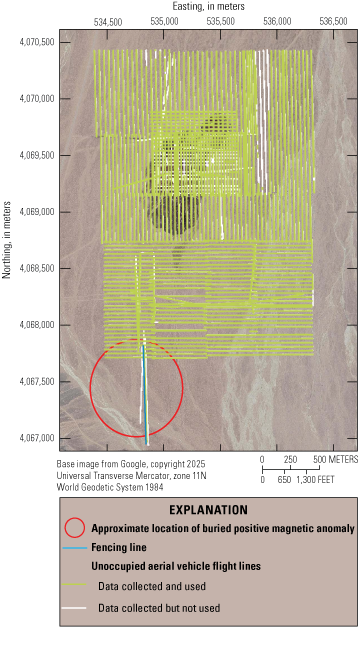
Map showing unoccupied aerial vehicle flight survey lines used for data collection, color-coded to indicate where data were either used or not used for analysis. Diagonal survey lines are ferry lines to and from the take-off and landing site. Where possible, data from the ferry lines were used as data for tie lines. The buried positive magnetic anomaly has been referred to colloquially in the scientific community since 1995 as the “Jerry Garcia anomaly.”
In the southwest corner of the surveyed region, there is a high positive magnetic anomaly (Langenheim, 1995; Connor and others, 1997; Perry, 2005) known informally and referred to colloquially in the scientific community since 1995 as the “Jerry Garcia anomaly.” This magnetic anomaly is not part of the lava flow associated with Little Cones, and it was generated by a buried sill or the upper part of an eroded volcanic conduit, with a depth beneath the ground surface of 148 m based on drilling and coring (Perry, 2005). Although the analysis of this magnetic anomaly is not part of the main investigation documented herein, the well-constrained signal was used to explore the use of magnetic data “fencing” in quantifying variations in the measured magnetic anomalies associated with the uncertainties in the flight altitude measurements. For the fencing, the UAV was flown at different altitudes along the same north-south line to capture the full vertical magnetic field profile. Repeated single-line passes were performed across the anomaly following the same horizontal trajectory but with the altitude AGL incrementally increased by 10 m with each pass, from 20 to 100 m AGL.
Structure From Motion Photogrammetry Survey
The topography of a smaller area (900 m x 900 m) surrounding the two scoria cones was mapped using the DJI Matrice 100 and a GoPro Hero 5 camera. This elevation survey was flown 80 m AGL. The camera was set to Linear FOV recording at 1-second time intervals, downward facing at ~5° forward of nadir. Seven ground control points (GCPs) were collected around Little Cones using a Trimble R10 RTX Receiver with Centerpoint correction service. In addition, a Global Navigation Satellite System profile, using the same Trimble receiver as above, was collected across Little Cones in a north-northeast–south-southwest direction to compare with the elevation model created from photogrammetry (appendix 1, fig. 1.1; Van Alphen and others, 2026).
Data Processing and Modeling
Data Processing
The raw data collected by the magnetometer were converted into American Standard Code for Information Interchange (ASCII) files containing the time of collection, the position, and the three components of the magnetic field measured by each magnetometer. The MagDrone R3 was attached to the UAV so that each end of the bar was equidistant from the center and placed perpendicular to the direction of flight. Hence, each measurement consisted of three components of the magnetic field, each 0.5 m from the center of the drone. We were unable to adequately extract attitude data from the inertial measurement unit on the UAV and thus remove the effect of platform motion on the x, y, and z sensor components. The total field of each sensor (being the square root of the sum of the square of each component) was therefore used and values from the two sensors were averaged to obtain a single magnetic field value.
An analysis of the measurement at each sensor indicated that the heading correction of the two single measurements was larger than the average value (possibly because of non-symmetric magnetic noise from the UAV, or a nonlevel attitude of the UAV to counteract cross winds) and that the average value had less scatter than the single component measurement. Following the analysis of Accomando and others (2021), the noise induced on the measurements by the electronic and mechanical noise of the UAV was evaluated. The motor of the UAV produced noise on the order of tens of nanoTeslas (nT) in the magnetic signal, concentrated at a frequency of about 50 Hz, and was greatly reduced at frequencies below 10 Hz (appendix 1, fig. 1.2); therefore, a low-pass filter was applied to the data to remove signal at frequencies higher than 5 Hz. Given an average flight speed of 8 meters per second, this filtering resulted in a resolution of 0.625 observations per meter.
A local magnetic base station was not available, so to account for diurnal variation in the magnetic field, we used observations from the INTERMAGNET geomagnetic observatory FRN in O’Neals, California (lat 37.0913° N., long 119.7193° W.), shifted by 752 seconds to account for the different longitudes of the two sites (St Louis, 2024). The use of a station 200 km away from the survey area is not ideal; however, the applicability of this approach was confirmed by cross-correlation of the magnetic signal of FRN with data from observatories FRD near Fredericksburg in Corbin, Virginia (lat 38.2100° N., long 77.3670° W.) and FUR in Fürstenfeldbruck, Germany (lat 48.1700° N., long 11.2800° E.), which had a similar quasi-dipole latitude with respect to International Geomagnetic Reference Field 13 (IGRF-13) in October 2019. The cross-correlation of the diurnal variation at station FRN with both FRD and FUR is shown in appendix 1, figure 1.3.
Flight lines were extracted from the data by comparing the horizontal components of the measured magnetic field to those of the expected local magnetic field. In the sensor configuration used for this study, the x-axis pointed to the right of the UAV and the y-axis was in the forward direction; hence, the x and y components of the UAV’s observed magnetic vector B were relative to the direction of the aircraft. The orientation of the UAV was computed by comparing the components of the UAV’s observed magnetic vector B to the horizontal components of the local magnetic field from the current World Magnetic Model (NOAA NCEI Geomagnetic Modeling Team, 2024). Individual flight lines were then extracted in the north-south and east-west directions. Only those lines longer than 100 m were retained, and the last 10 m of each line was removed to eliminate noise caused by the acceleration of the UAV during changes in flight direction. The flight lines used in the following analysis are shown in figure 3.
The geolocation of each measurement was obtained using the internal GPS of the Sensys MagDrone instrument. Collecting data for several hours with the UAV stationary, we observed that the internal GPS has a measurement repeatability of about 4 m horizontal and 8 m vertical. This repeatability was assumed to be a good proxy for the uncertainties associated with the GPS unit in the magnetic sensor, although this static test did not account for changes in aircraft attitude and potential shielding during flight conditions. An analysis of the location of each measurement indicated that in high-wind conditions (greater than [>]10 knots), the UAV had difficulty maintaining a fixed 40-m altitude AGL (as defined by the SRTM topography). Although a draped survey at 40 m AGL was flown, all the points that deviated from 40 m AGL were removed to avoid potential noise resulting from variation between planned and actual flight altitude, allowing a buffer of ±7 m to account for the precision of the GPS sensor. An analysis of the UAV's trajectory indicated that the flights were mostly within 1 m of the planned flight altitude. It was not possible to synchronize the geolocalization of the UAV with the magnetic data collection, necessitating the use of the internal GPS unit of the magnetometer. The 7-m buffer is a compromise derived by a comparison of the magnetometer position to the UAV flight path. An analysis of the fencing data confirmed that the altitude AGL of the flight had an average bias of 2 ±4 m, and that the uncertainties associated with the magnetic anomalies introduced by the vertical measurement were on the order of 15–50 nT. Appendix 1 discusses the fencing technique in greater detail.
We checked the crossing points provided by ferry lines and those provided by the north-south and east-west lines in the area of high-resolution data collection near the cones. For 267 crossing points, the horizontal separation was less than 1 m. Apart from seven points where the difference was ~100 nT (which are in areas of large gradients), the average difference of the crossing points was −0.5 nT, with a standard deviation of 21 nT and a range of measurement differences between –61 and +49 nT. Overall, survey error was <60 nT.
The geolocation of the remaining dataset was then transformed into Universal Transverse Mercator (zone 11 north) coordinates for ease of processing. To facilitate the interpretation and modeling of this dataset, the data were gridded using a minimum curvature method (Wessel and others, 2019) with a grid spacing of 10 m. Following the method of Leblanc and Morris (2001), the gridded dataset was micro-leveled using a wavelet method. Lastly, to remove the tectonic signal caused by local faulting, the dataset was detrended using a plane that best fit the observations of the micro-levelled magnetic field. All of the analysis and discussion that follows refers to the gridded, micro-levelled, and detrended dataset as the “observed” magnetic field, which is shown in figure 4B.
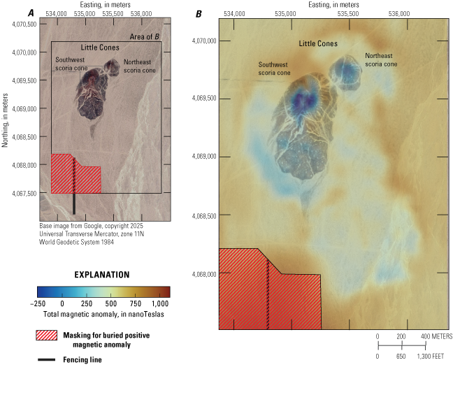
A, Satellite image showing Little Cones. B, Magnetic map after filtering, gridding, levelling, and detrending of unoccupied-aerial-vehicle-collected data. The buried positive magnetic anomaly has been referred to colloquially in the scientific community since 1995 as the “Jerry Garcia anomaly,” and is not a part of the scoria cone system and was not used for inversions.
Three-Dimensional Data Inversion
The gridded, levelled, and detrended observed field (fig. 4B) was inverted to map the buried lava flow and the magnetic field induced by the cones. For the forward modeling, the source of the magnetic anomaly was approximated by means of triangular prisms of different thicknesses, and the resulting magnetic field at the observation point was computed using the method described by Plouff (1976). We ran a model using the full dataset, and two models at higher spatial resolutions for the southwest scoria cone and the southern end of the anomaly. The full dataset (lava flow and cones) was simulated through a tessellation with triangles having a maximum area of 1300 square meters (m2), representing a spatial resolution of the lava flow of about 50 m. For the region around the largest cone (the southwest scoria cone), the maximum area was 400 m2, or about 30 m resolution, and for the southern extent of the magnetic anomaly the maximum area was 800 m2, corresponding to a resolution of about 40 m.
The lower base of the prisms was assumed to rest on the alluvial paleosurface over which the lava from Little Cones erupted, and the paleoplain was assumed to be parallel to the current surface, which slopes at approximately 0.6–0.7° to the south-southeast. Given the correction to the observed data and the modality of data collection (in other words, constantly flying 40 m above the current surface), the paleoplain was assumed to be a planar surface in the inversion process.
Using the local sedimentation-rate evidence and magnetic inversion, Stamatakos and others (1997) suggested that the depth of the paleosurface is approximately 15 m. The paleosurface depth was allowed to be a free parameter in the inversion, varying from 10 to 30 m. For the buried lava flow, the upper surface of the prisms was allowed to vary, and this value was used to estimate the thickness of the lava flow. For the cones and the exposed part of the lava flow (that is, where the thickness of the prism is higher than the depth of the paleoplain), the top surface was constrained to match the observed topography. This constraint implies that the magnetic anomaly contribution from the prisms associated with the outcropping lava flow and cones was simulated as a topographic correction, with the only free parameters being the intensity of remanent magnetization and the depth of the paleoplain. For the high-resolution inversion of the cone, models were run for which the depth to the bottom of the prisms could vary deeper than the paleoplain to test for the presence of feeder dikes.
We assumed that the intensity of remanent magnetization is constant within each triangular prism and that there are two different intensities of remanent magnetization: one representing the value for all the prisms representing the lava flow and one for all the prisms representing the cone. For the inversion, a prism is defined as belonging to the cone if the observed ground elevation at the center of the prism exceeds 886 m on the DEM (dark yellow in fig. 5). This results in a shape resembling an almost circular cone. The two intensities of remanent magnetization are free parameters in the inversion. The values for the intensity of magnetization were allowed to vary from 0.2 to 10 amperes per meter (A/m).
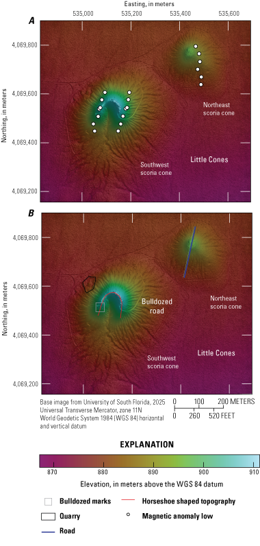
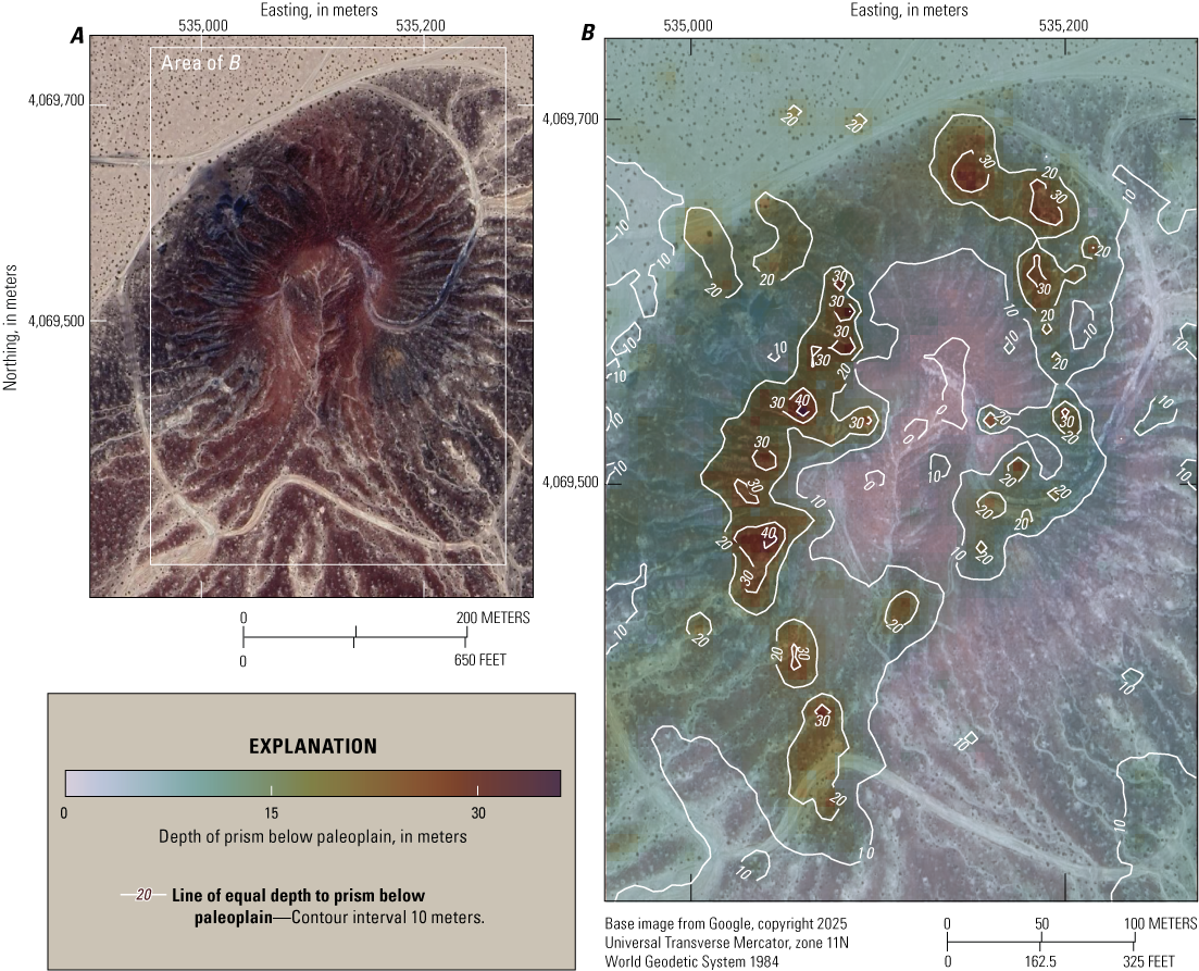
Photogrammetry-based digital elevation model (DEM) of Little Cones, with associated magnetic anomaly lows and selected anthropogenic features. A, Geographic locations of magnetic anomaly lows plotted in figure 6. B, Location of small quarry, bulldozed road, and bulldozer marks on and near the southwest cone, and location of road that crosses the summit of the northeast cone. DEM data are available in Van Alphen and others (2026).
The inversion was run using a Python code that minimizes the residuals of the synthetic field with respect to the observed field through both the Nelder-Mead (Nelder and Mead, 1965; Gao and Han, 2012) and Broyden-Fletcher-Goldfarb-Shanno (BFGS; Nocedal and Wright, 2006) methods provided by SciPy. The code was implemented using the NUMBA library to run on an intel 9 processor with Nvidia 2090 graphics processing unit and 64 gigabytes of memory. Each inversion of the full gridded and detrended dataset for the full tessellation took approximately 132 hours. The inversion parameters and associated values used in the inversion model are shown in table 1.
Table 1.
Inversion parameters for scoria cone and lava flow inversion model.[IGRF, International Geomagnetic Reference Field; A/m, ampere per meter; m, meter; DEM, digital elevation model]
Stamatakos and others (1997) provides estimates for both the inclination and declination of Little Cones.
Digital Terrain Modeling
Images from the GoPro Hero 5 camera were collected once per second. For ease of processing, every fifth image (5-second sampling) was extracted. Agisoft Metashape was used for structure-from-motion (SfM)-photogrammetry data processing (Agisoft LLC, 2022). Initial camera positions were taken from the GPS inside the GoPro for initial alignment, and then the seven high-precision ground control points were used to georeference the model. The high-density point cloud model and input images were used to produce the DEM shown in figure 5 and orthophoto at a resolution of 16 centimeters per pixel (Van Alphen and others, 2026).
Results
Qualitative Results
The high resolution (16 centimeters per pixel) DEM (fig. 5; Van Alphen and others, 2026) shows that much of the erosion at both Little Cones is focused in channels and rills present on all flanks of the cones. Obvious signs of human use and modification of both cones include, for example, a small quarry on the northwestern flank of the southwest scoria cone; a north-south dirt road that crosses the northeast scoria cone; a dirt road that leads up to the top of the southwest scoria cone; and markings indicating the movement of heavy machinery (fig. 5B). The morphology of the southwest scoria cone is that of a horseshoe crater open to the south-southwest.
The observed negative magnetic anomaly is most prominent at the two cones, with negative values extending to the south beyond the subaerial outcrops of basalt (fig. 4B). As noted by Connor and others (1997), these negative values clearly outline the presence of a reversely magnetized lava flow underneath the current ground surface. Assuming that the magnitude of the magnetic anomaly is proportional to the thickness of the flow, a possible thicker flow is observed in the direction of the open side of the crater in the southwest scoria cone and a longer thinner flow is observed to the south of the northeast scoria cone.
The internal structure of the cone can be investigated on the basis of the magnetic profiles (fig. 6) and the magnetic map (fig. 4). The magnetic profiles (fig. 6) show small superposed magnetic lows across both cones. At the southwest scoria cone, the lows follow a north-northeast–south-southwest trend, whereas at northeast scoria cone, the lows follow a north-south trend. These orientations are consistent with the overall northeast-southwest alignment of volcanic cones within Crater Flat (Connor and others, 2000; fig. 1A). The magnetic lows along the profile lines bracket the topographic low of the open crater at the southwest scoria cone (fig. 5A).
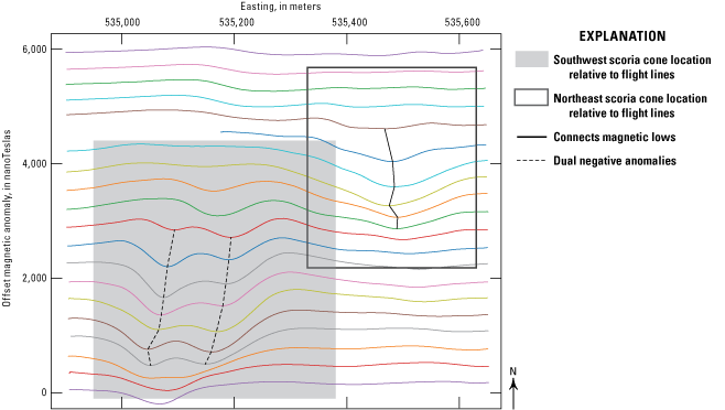
Graph showing east-west survey transects across Little Cones that are offset for visualization, such that the lowest of the magnetic anomaly lines is the southernmost profile, and successively greater anomaly lines are successively farther north. The lines connecting the magnetic lows on the graph correspond to the locations of the magnetic lows shown in figure 5A.
Quantitative Results
Paleoplain Depth and Magnetization
The depth of the paleoplain, thickness of the lava flow, and magnitude of the magnetization are closely related parameters in magnetic field modelling. This relation arises from the inherent non-uniqueness present in all potential field measurements (Telford and others, 1990). The deeper the source of the measured magnetic field, the weaker the induced field at the surface, resulting in longer wavelengths of the observed signal. For the buried part of the flow, there are two options to reproduce the observed signal while accommodating a deeper paleoplain: either increase the magnetization or allow larger variation of the thickness of the lava flow. For the exposed part of the flow, a deeper paleoplain would increase the volume of the magnetic field source, producing a greater magnetic anomaly. Therefore, to reproduce the observed field while accommodating a deeper paleoplain, it is necessary to reduce the magnetization. Having such opposite requirements for the buried and exposed parts of the flow can help to better constrain our inversion.
Although we could theoretically fit the observations by varying either the gradient of the edges of the lava flow or the magnetization value while changing the depth of the paleoplain, all of the inversions prefer the latter. Both the Nelder-Mead and BFGS schemes were used for the inversion, and independent of the initial thickness of the buried lava flow used to initialize the model, all of the inversions converge toward a larger magnetization of the basalt flow at a greater paleoplain depth while keeping the best fitting thickness of the lava flow almost constant.
To better understand the influence of paleoplain depth, several inversions were conducted by fixing the paleoplain depth at different values while solving for the remaining parameters. The best-fitting values of magnetization range from 10 A/m for a paleoplain 30 m deep to 0.9 A/m for a paleoplain 10 m deep. Although all the best-fit models having paleoplain depths ranging from 24 to 12 m yield approximately the same average residuals and are statistically indistinguishable, the spatial variation in the residuals was observed to change across all models. Models with greater paleoplain depths tend to produce larger misfits in the area of the exposed lava flow while fitting the flow toes very well. In contrast, models with shallower paleoplain depths tend to fit the exposed flow better but have larger misfits at the flow toes. To preserve the correct observed anomaly at the flow toes for paleoplain depths less than 10 m, either the intensity of magnetization would need to be too low (of the order of 0.6 A/m or less) or the thickness of the flow would need to be extremely low (less than half a meter). Models having paleoplain depths between 17 and 15 m appear to have a more homogeneous misfit throughout the entire modeled area. To better compare results of this study with those of previous studies (Stamatakos and others, 1997; Valentine and others, 2006), a paleoplain depth of 15 m was utilized for the rest of the analysis, as suggested by Stamatakos and others (1997). For models having a paleoplain depth of 15 m, the optimal intensity of magnetization for the lava flow, ranging from 0.6 to 2 A/m, is statistically indistinguishable, and the lava flow morphologies observed for models using all of these intensities of magnetization are similar. The following discussion presents the results using an intensity of magnetization for the lava flow of 1 A/m.
Regardless of the depth of the paleoplain, the results indicate that the magnetization of the exposed cones cannot exceed 0.6 A/m without producing a signal significantly larger than the one observed. Indeed, our best-fit models for the magnetization of the cones range from 0.35 to 0.6 A/m, increasing as the paleoplain depth decreases from 27 to 10 m. This range is significantly lower than the measured magnetization of exposed basalts in the region, which ranges from 7.5 to 15 A/m (Champion, 1991). This finding indicates that the bulk magnetization of the cones at the outcrop scale is less than the magnetization determined by paleomagnetic sampling, likely because of the random accumulation of scoria after it cooled below the Curie temperature.
Lava Flow Thickness Inversion
The inversion for a paleoplain depth of 15 m, with a magnetization for the cone of 0.6 A/m and for the lava flow of 1 A/m, is shown in figure 7A–C. The residual for this inversion is presented in figure 7C, which represents the difference between the calculated magnetic anomaly (fig. 7B) and observed magnetic anomaly (fig. 7A). The average residual for this inversion is 6 nT, with a standard deviation of 22 nT. The largest residuals are in and near the southwest scoria cone. Part of this residual is related to the size of the modeled prisms (discussed later in this section). The observed magnetic anomaly at the southwest scoria cone consists of two distinct, approximately north-south trending sigmoid-shaped negative anomalies (fig. 7A). The size of the prisms for the global inversion precludes resolving these two features, leading to a calculated anomaly that is circular and resembles the general shape of the cone. Another region with a larger-than-average residual lies southwest of the southwest scoria cone, where the lava flow is thickest and the cone has a breach-like morphology. This residual is related to the choice of the lower magnetization definition for the cone and the decision to assume only two different magnetizations for the cone and for the lava flow. It is likely that the actual transition is more gradual and that the original shape of the cone was not circular; rather, the breach is a feature of the cone that was present during the full eruption, as observed in recent eruptions in Hawaii and Iceland (Neal and Anderson, 2020; Eibl and others, 2024). All of these effects are not modeled in our inversion, which assumes the presence of only two main bulk magnetizations constant on each prism.
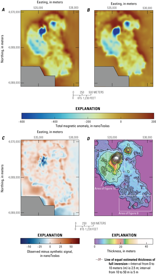
Maps showing (A) Observed signal, (B) synthetic signal, (C) difference between observed and synthetic signal for the full inversion and (D) estimated thickness of the full inversion (fig. 8 shows greater detail).
The final thickness map (figs. 7D, 8) includes the cone, the exposed lava flow, and the buried lava flow sections. This map represents the combined thickness of the volcanic products and not explicitly the topography of the lava flow surface. (In other words, topography would only reflect the upper surface variation, whereas the thickness allows for variation of both the upper and lower surfaces.) The thickness map can be used to reconstruct the eruptive history in the same manner one would map active or recent lava flows using topography.
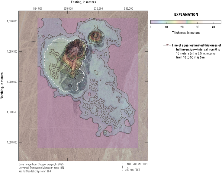
Maps showing thickness of Little Cones and flows for the full preferred inversion. The white outline on the map highlights the 7.5-meter contour, which in the interpretation documented herein represents lava erupted onto the inflated surface of the lava flow.
A higher resolution model was used to estimate the thickness of the lava flow in two smaller areas: the southern end of the lava flow (fig. 9A–D) and in the area of the southwest Little Cone (fig. 10A–D). Both models use the same paleoplain depth of 15 m below the surface. The intensity for the southwest scoria cone is fixed at 0.6 A/m and the intensity for the toe is fixed at 1 A/m. Although the low-resolution model is not able to reproduce the observed sigmoid shape of the anomaly, the high-resolution model for the cone can resolve this feature (fig. 10D).
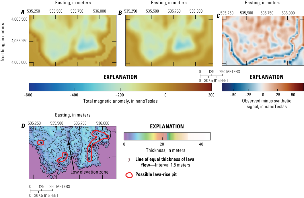
A, Observed signal. B, Synthetic signal. C, Difference between observed and synthetic signal for the higher-resolution model in the southernmost extent of the lava flow (location shown in fig. 7). Positive anomalies in the northern section are caused by edge effects. D, Estimated thickness of the southernmost extent of the concealed lava flow. Low-elevation zone indicates area of possibly uninflated lava.
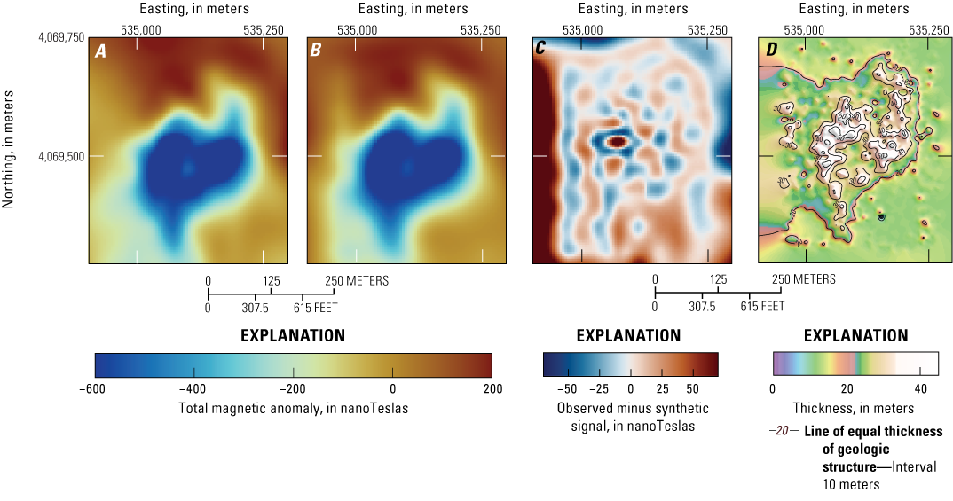
A, Observed signal. B, Synthetic signal. C, Difference between observed and synthetic signal for the higher-resolution model in the area around the southwest scoria cone of Little Cones (location shown in fig. 7). D, Estimated deposit thickness in the southwest scoria cone area.
The total erupted volume was estimated by summing the modeled thickness (figs. 7D, 8) of each prism across the entire extent of the map. The total flow volume for a model that assumes a paleoplain depth of 15 m, with a magnetization intensity of 0.6 A/m for the cone and 1 A/m for the lava flow, is approximately 0.016 km3. Uncertainties inherent to the inversion model—for example, the comparison of results from Nelder-Mead with those from BFGS, or different initializations of the recursive models—can account for a volume variation of approximately 15 percent (about 0.002 km3). The variations in the paleoplain and the intensity of magnetization described in the previous section can lead to volume variations of up to 0.01 km3, with larger volumes associated with lower magnetization intensity. The volume estimated by the results of this study is roughly half of the volume calculated by Valentine and others (2006) based on their assumption that the magnetic anomaly represents the lava flow area and that the lava flow maintains a constant thickness of 10 m beneath 10 m of alluvium. Despite the significant approximations in the calculations of Valentine and others (2006), the differences between their model and the model in this study are well within the uncertainties of our inversion.
Discussion
Although the inversion does not improve estimates of the total eruption volume for Little Cones, it does reveal details about the flow morphology and provides an opportunity to interpret the eruption from a volcanological perspective. The spatial relations and thickness maps from this study can be used to reconstruct a possible order of events during the eruption and use the lava flow morphology to infer emplacement mechanisms for the lava flow field.
Sequence of Events
We propose a volcanological model of the eruption as follows (figs. 11, 12). The initial dike surfaces as a northeast-southwest-trending fissure (figs. 11A, 12A). A pāhoehoe sheet flow erupts at high effusion rates, spreading somewhat radially with a dominant southward advance, guided by the paleoplain slope (figs. 11B, 12B). As effusion rates decrease, the sheet flow begins to cool and inflate in places but not uniformly (Bakowski, 2025; figs. 11C, 12C), producing a lava pad onto which new eruptive material flows (Valentine and others, 2006). Following the onset of inflation, eruptive activity localizes at two points along the fissure, corresponding to the development of the two Little Cones volcanoes and associated secondary lava pulses (fig. 11C). This spatial concentration of eruptive activity effectively reduces the lava supply sustaining inflation, resulting in a pronounced decline in surface uplift of the initial lava flow. As inflation diminishes, the viscoelastic crust of the flow progressively solidifies and becomes increasingly brittle, ultimately leading to the cessation of inflation (Bakowski, 2025; fig. 12D). Subsequent eruption pulses form the two scoria cones from spatter and agglutinate, eventually producing new lava flows around the cones on the surrounding, previously erupted and inflated lava flow surfaces. The path that these later-stage lava flows take is determined by the topography created by inflation. For example, the southern section of the initial lava flow experienced a higher degree of inflation compared to the northern section. This created a topographic high near the southern edge of the southwest scoria cone (fig. 12C–D) and caused late-stage lava pulses to be diverted to the north and northwest in a fan-like manner (figs. 11E, 12E). In addition, the topographic map and the magnetic signal indicate that the southern portion of the southwest scoria cone remained an open channel (Neal and Anderson, 2020; Eibl and others, 2024), influencing the direction of the lava flow. We found no evidence of rafted material in the exposed geology or in the magnetic mapping and inversion, indicating that the cone developed with, and maintained, an open flank. This interpretation builds on the ideas of Valentine and others (2006).
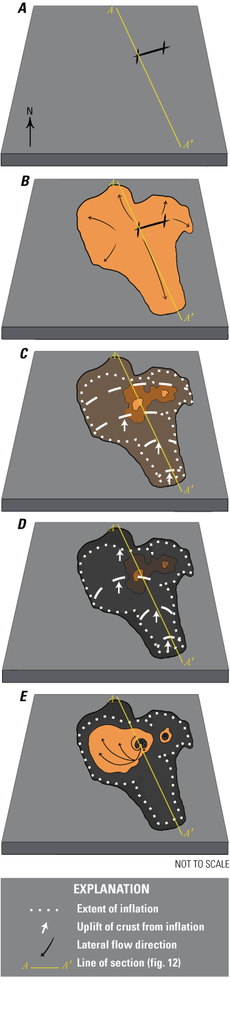
Conceptual block diagrams showing order of events at Little Cones. A, Initial fissure complex formation. B, Emplacement of sheet flow. C, Eruption continues, concentrates, and lava flow begins to inflate. D, Cone building creates two cones while flow inflation ceases. E, Late-stage lava flows are directed around the southwest scoria cone of Little Cones by post-inflation topography. Time steps here do not correspond to those in figure 12.
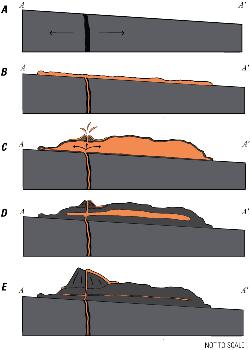
Schematic cross-section showing order of events at the southwest scoria cone of Little Cones. A, Initial fissure formation. B, Emplacement of a sheet flow. C, Inflation begins, which aids in concentrating subsequent pulses, and scoria cones begin to form above areas of focused venting. D, Inflation ceases, and flow concentrates around the cones. E, Cones fully formed, with southwest scoria cone having an open channel to the south. Time steps here do not necessarily correspond to those in figure 11.
Thickness Map Interpretations
The initial eruptive event at Little Cones is interpreted to issue from a group of fissure segments to explain the initial coherent sheet flow indicated by the 2.5-m contour in the full field thickness map (fig. 8). Specifically, the lava erupted from all fissure segments to produce the sheet flow. Moving up one contour to the 5-m line, the inflated portion of the initial sheet flow is evident, with the thickest part being southeast of the southwest scoria cone. Further eruptions from the southwest scoria cone are then directed around the cone, forming the thickest part of the flow surface. The northeast scoria cone produced relatively little lava after the initial flow emplacement. Perhaps a full cone formed with a lava lake that never breached or overtopped its crater rim. This interpretation is supported by the high-resolution DEM, which shows slopes steepening upward on the upper part of the northeast scoria cone, consistent with a dense, difficult-to-erode unit at the top of the cone (Van Alphen and others, 2026). It is also possible that the eruption became more focused at the southwest scoria cone, accounting for the remaining activity during the event. Our inversion of the southern terminus of the flow shows separation of the toe into possibly two segments and contains inflationary features within the toe (fig. 9D).
The southern terminus of the initial sheet flow displays significant topographic variation (fig. 9D). Specifically, the flow margins have a relief of 3 m, whereas the interior part of the flow reaches a greater relief of approximately 6.0–7.5 m. This variation is likely caused by differences in the amount of inflation experienced in this area of the flow—areas with the lowest current elevation experienced little to no inflation, whereas the currently higher-elevation areas experienced the most inflation. The inflated areas appear to be somewhat interconnected, forming features that reflect the preferred pathways of lava delivery during inflation. These connected zones are best described as lava rises (Walker, 1991). Surrounding the lava rises are circular, uninflated features. These features can either form in isolation, scattered individually across the surface, or form in close proximity to one another, sometimes creating recognizable patterns. Given the inferred inflation of this area and the distinctive morphology of these features, it is plausible that they represent lava-rise pits (fig. 9D), similar to those observed on inflated Holocene lava flows (Bakowski, 2025). Their formation probably involved the initial sheet flow encountering obstacles around which the lava diverted. As the flow inflated, these obstacles remained uninflated, leading to topographic inversions and the development of lava-rise pits (Walker, 1991). In addition to the lava-rise pit features, this area features a prominent low-elevation zone that trends north-south through the center (fig. 9D). This depression likely represents a portion of the flow that did not undergo inflation. The overall structure and morphology of this area and these features strongly support our interpretation that differential flow inflation played a central role in shaping the final topography of the flow’s southern terminus.
The high-resolution inversion of the southwest scoria cone identifies two en echelon north-south trending structures that match the observed sigmoid signal (fig. 10A, D). These features are thicker than expected from the observed height of the cone above the current surface (fig. 13A). The en echelon bodies can be interpreted either as a deeper structure below the cone, like a feeder dike, or as a more magnetic body within the cone, including agglutinated material.
A, Orthophoto background with, B, depth inversion map.
Calculated Flow Characteristics
The modeled lava flow geometry can serve as a basis to estimate the initial flow viscosity and yield strength. A cooling-limited lava flow field is assumed because the eruption continued after emplacement of the initial approximately 3-m-thick sheet flow. First, the effusion rate, Q, is calculated for the initial flow sheet based on Chevrel and others (2013):
whereGz
is the Grätz number (a dimensionless number that relates the rate at which heat is lost from the lava flow to the distance the lava flow has traveled from the vent),
is the bulk thermal diffusivity,
L
is the lava flow length (from the southwest scoria cone to the toe),
w
is the lava flow width, and
h
is the average flow thickness.
g
is gravitational acceleration;
ρ
is lava density, assumed to be 2,600 ±50 kilograms per cubic meter; and
β
is the paleoslope.
From the inversion model, the volume of the early emplaced lava flow sheet is inferred to be approximately 0.00678 km3, given a paleoplain depth of 15 m; thus, it took approximately 3–13 hours to emplace the initial flow sheet, which is the maximum extent of lava inundation for this eruption. Following emplacement of this cooling-limited lava flow, it is unclear whether pauses in the eruption were associated with inflation of the flow field, the construction of the cones, or subsequent lava flows, and the total eruption duration is not estimated.
The value added in conducting the UAV-borne magnetic survey of Little Cones is primarily the increased resolution of the lava flow field, the morphology of which yields constraints on the sequence of events during the eruption and allows eruption source parameters to be estimated for the lava flow field, such as effusion rate, that may be useful in lava flow hazard models.
Conclusions
This report presents the results of an unoccupied aerial vehicle fluxgate magnetic survey of Little Cones, Nevada, scoria cones and associated lava flows buried by alluvium. A nonlinear inversion reveals the morphology of the lava flow field and near-vent structures. The total volume of the cones and lava flow field was modeled as approximately 0.016 cubic kilometer. The southern flow toe reveals inflation structures, whereas the southwest scoria cone is characterized by a coherent sigmoidal structure beneath the edifice that may indicate a feeder structure or the presence of agglutinate. We conclude that the lava flow field was built from an initial sheet flow, then inflated by additional lava pulses. The eruption then became concentrated at the cones, with all subsequent lava flows confined to the area around them—primarily around the southwest scoria cone. These results emphasize a novel interpretation related to the formation of scoria cones and associated lava flows in the Crater Flat basin, highlighting the role of flow inflation and eruption concentration along a fissure system, both of which shape the subsurface and surface morphology of Little Cones. Combining the lava flow geometry from the inversion of unoccupied-aerial-vehicle-derived magnetic data with a sequence of events allows constraint of the initial eruption characteristics and calculation of eruption source parameters such as effusion rates. These parameters are a key input to lava flow inundation hazard models and can help better inform these predictive models.
References Cited
Accomando, F., Vitale, A., Bonfante, A., Buonanno, M., and Florio, G., 2021, Performance of two different flight configurations for drone-borne magnetic data: Sensors, v. 21, no. 17, article 5736, accessed February 2025 at https://doi.org/10.3390/S21175736.
Athens, N.D., Ponce, D.A., Jayko, A.S., Miller, M., McEvoy, B., Marcaida, M., Mangan, M.T., Wilkinson, S.K., McClain, J.S., Chuchel, B.A., and Denton, K.M., 2014, Magnetic and gravity studies of Mono Lake, east-central, California: U.S. Geological Survey Open-File Report 2014–1043, 14 p., accessed May 2025 at https://doi.org/10.3133/ofr20141043.
Bacon, C.R., 1982, Time-predictable bimodal volcanism in the Coso Range, California: Geology, v. 10, no. 2, p. 65–69, accessed February 2025 at https://doi.org/10.1130/0091-7613(1982)10<65:TBVITC>2.0.CO;2.
Bebbington, M.S., 2014, Long-term forecasting of volcanic explosivity: Geophysical Journal International, v. 197, no. 3, p. 1500–1515, accessed June 2021 at https://doi.org/10.1093/gji/ggu078.
Blakely, R.J., Langenheim, V.E., Ponce, D.A., and Dixon, G.L., 2000, Aeromagnetic survey of the Amargosa Desert, Nevada and California—A tool for understanding near-surface: U.S. Geological Survey Open-File Report 00-188, 32 p., accessed January 2020 at https://doi.org/10.3133/ofr2000188.
Carr, W.J., and Parrish, L.D., 1985, Geology of drill hole USW VH-2, and structure of Crater Flat, southwestern Nevada: U.S. Geological Survey Open-File Report 85-475, 41 p., accessed February 2022 at https://doi.org/10.3133/ofr85475.
Champion, D.E., 1991, Volcanic episodes near Yucca Mountain as determined by paleomagnetic studies as Lathrop Wells, Crater Flat, and Sleeping Butte, Nevada, in Annual American Nuclear Society (ANS) international high level radioactive waste management conference, 2nd, Las Vegas, NV., Apr. 28–May 3, 1991, High level radioactive waste management—Proceedings of the second annual international conference: New York, N.Y., American Society of Civil Engineers, p. 61–67, accessed June 2021 at https://inis.iaea.org/records/33wm3-y6545.
Champion, D.E., Lanphere, M.A., and Kuntz, M.A., 1988, Evidence for a new geomagnetic reversal from lava flows in Idaho—Discussion of short polarity reversals in the Brunhes and late Matuyama polarity chrons: Journal of Geophysical Research, v. 93, B10, p. 11667–11680, accessed February 2022 at https://doi.org/10.1029/JB093IB10p11667.
Chevrel, M.O., Platz, T., Hauber, E., Baratoux, D., Lavallée, Y., and Dingwell, D.B., 2013, Lava flow rheology—A comparison of morphological and petrological methods: Earth and Planetary Science Letters, v. 384, p. 109–120, accessed May 2025 at https://doi.org/10.1016/j.epsl.2013.09.022.
Civico, R., Ricci, T., Scarlato, P., Taddeucci, J., Andronico, D., Del Bello, E., D’Auria, L., Hernández, P.A., and Pérez, N.M., 2022, High-resolution digital surface model of the 2021 eruption deposit of Cumbre Vieja volcano, La Palma, Spain: Scientific Data, v. 9, no. 1, accessed May 2025 at https://doi.org/10.1038/s41597-022-01551-8.
Connor, C.B., and Hill, B.E., 1995, Three nonhomogeneous Poisson models for the probability of basaltic volcanism—Application to the Yucca Mountain region, Nevada: Journal of Geophysical Research, v. 100, no. B6, p. 10107–10125, accessed February 2022 at https://doi.org/10.1029/95JB01055.
Connor, C.B., Lane-Magsino, S., Stamatakos, J.A., Martin, R.H., LaFemina, P.C., Hill, B.E., and Lieber, S., 1997, Magnetic surveys help reassess volcanic hazards at Yucca Mountain, Nevada: Eos (Washington, D.C.), v. 78, no. 7, p. 73–78, accessed January 2020 at https://doi.org/10.1029/97EO00049.
Connor, C.B., Stamatakos, J.A., Ferrill, D.A., Hill, B.E., Ofoegbu, G.I., Conway, F.M., Sagar, B., and Trapp, J., 2000, Geologic factors controlling patterns of small-volume basaltic volcanism—Application to a volcanic hazards assessment at Yucca Mountain, Nevada: Journal of Geophysical Research, v. 105, no. B1, p. 417–432, accessed January 2020 at https://doi.org/10.1029/1999JB900353.
Courtland, L., Kruse, S., and Connor, C., 2013, Violent strombolian or not? Using ground-penetrating radar to distinguish deposits of low- and high-energy scoria cone eruptions: Bulletin of Volcanology, v. 75, no. 12, accessed May 2021 at https://doi.org/10.1007/s00445-013-0760-z.
Crameri, F., 2023, Scientific colour maps (8.0.1): Zenodo, accessed May 2025 at https://doi.org/10.5281/zenodo.8409685.
Dietterich, H.R., Grant, G.E., Fasth, B., Major, J.J., and Cashman, K.V., 2022, Can lava flow like water? Assessing applications of critical flow theory to channelized basaltic lava flows: Journal of Geophysical Research—Earth Surface, v. 127, no. 9, article e2022JF006666, 26 p., accessed April 2026 at https://doi.org/10.1029/2022JF006666.
Eibl, E.P.S., Thordarson, T., Moreland, W.M., Gudnason, E.Á., Höskuldsson, Á., Hersir, G.P., and Heimann, S., 2024, Illuminating the transition from an open to a semi-closed volcanic vent system through episodic tremor duration and shape: Journal of Geophysical Research. Solid Earth, v. 129, no. 5, accessed April 2025 at https://doi.org/10.1029/2023JB028323.
Farr, T.G., Rosen, P.A., Caro, E., Crippen, R., Duren, R., Hensley, S., Kobrick, M., Paller, M., Rodriguez, E., Roth, L., Seal, D., Shaffer, S., Shimada, J., Umland, J., Werner, M., Oskin, M., Burbank, D., and Alsdorf, D.E., 2007, The shuttle radar topography mission: Reviews of Geophysics, v. 45, no. 2, accessed October 2022 at https://doi.org/10.1029/2005RG000183.
Fleck, R.J., Turrin, B.D., Sawyer, D.A., Warren, R.G., Champion, D.E., Hudson, M.R., and Minor, S.A., 1996, Age and character of basaltic rocks of the Yucca Mountain region, southern Nevada: Journal of Geophysical Research, v. 101, no. B4, p. 8205–8227, accessed February 2022 at https://doi.org/10.1029/95JB03123.
Gallant, E., Richardson, J., Connor, C., Wetmore, P., and Connor, L., 2018, A new approach to probabilistic lava flow hazard assessments, applied to the Idaho National Laboratory, eastern Snake River Plain, Idaho, USA: Geology, v. 46, no. 10, p. 895–898, accessed April 2020 at https://doi.org/10.1130/G45123.1.
Gao, F., and Han, L., 2012, Implementing the Nelder-Mead simplex algorithm with adaptive parameters: Computational Optimization and Applications, v. 51, no. 1, p. 259–277, accessed April 2025 at https://doi.org/10.1007/s10589-010-9329-3.
George, O.A., McIlrath, J., Farrell, A., Gallant, E., Tavarez, S., Marshall, A., McNiff, C., Njoroge, M., Wilson, J., Connor, C., Connor, L., and Kruse, S., 2015, High-resolution ground-based magnetic survey of a buried volcano—Anomaly B v. 1: Amargosa Desert, NV, Statistics in Volcanology, p. 1–23, accessed February 2022 at https://doi.org/http://dx.doi.org/10.5038/2163-338X.1.3.
Heizler, M.T., Perry, F.V., Crowe, B.M., Peters, L., and Appelt, R., 1999, The age of Lathrop Wells volcanic center—An 40Ar/39Ar dating investigation: Journal of Geophysical Research, v. 104, no. B1, p. 767–804, accessed February 2022 at https://doi.org/10.1029/1998JB900002.
Horng, C.S., Lee, M.Y., Palike, H., Wei, K.Y., Liang, W.T., Iizuka, Y., and Torii, M., 2002, Astronomically calibrated ages for geomagnetic reversals within the Matuyama chron: Earth, Planets, and Space, v. 54, no. 6, p. 679–690, accessed may 2025 at https://doi.org/10.1186/BF03351719.
Hulme, G., 1974, The Interpretation of Lava Flow Morphology: Geophysical Journal International, v. 39, no. 2, p. 361–383, accessed may 2025 at https://doi.org/10.1111/j.1365-246X.1974.tb05460.x.
Idaho National Laboratory [INL], 2024, Idaho National Laboratory integrated multisite SSHAC Level 3: Probabilistic volcanic hazard assessment: INL/RPT-24-78997, accessed May 2025 at https://www.osti.gov/biblio/2497337.
Kereszturi, G., Jordan, G., Németh, K., and Dóniz-Páez, J.F., 2012, Syn-eruptive morphometric variability of monogenetic scoria cones: Bulletin of Volcanology, v. 74, no. 9, p. 2171–2185, accessed January 2020 at https://doi.org/10.1007/s00445-012-0658-1.
Kiyosugi, K., Horikawa, Y., Nagao, T., Itaya, T., Connor, C.B., and Tanaka, K., 2014, Scoria cone formation through a violent Strombolian eruption—Irao Volcano, SW Japan: Bulletin of Volcanology, v. 76, no. 1, accessed June 2021 at https://doi.org/10.1007/s00445-013-0781-7.
Kuntz, M.A., Champion, D.E., Spiker, E.C., and Lefebvre, R.H., 1986, Contrasting Magma Types and Steady-State, Volume-Predictable, Basaltic Volcanism along the Great Rift, Idaho: Geological Society of America Bulletin, v. 97, no. 5, p. 579–594, accessed September 2022 at https://doi.org/10.1130/0016-7606(1986)97<579:CMTASV>2.0.CO;2.
La Femina, P.C., Connor, C.B., Stamatakos, J.A., and Farrell, D.A., 2002, Imaging an active normal fault in alluvium by high-resolution magnetic and electromagnetic surveys: Environmental & Engineering Geoscience, v. 8, no. 3, p. 193–207, accessed June 2023 at https://doi.org/10.2113/8.3.193.
Langenheim, V.E., 1995, Magnetic and gravity studies of buried volcanic centers in the Amargosa Desert and Crater Flat, southwest Nevada: U.S. Geological Survey Open-File Report 95-564, 37 p., accessed February 2022 at https://doi.org/10.3133/ofr95564.
Leblanc, G.E., and Morris, W.A., 2001, Denoising of aeromagnetic data via the wavelet transform: Geophysics, v. 66, no. 6, p. 1793–1804, accessed July 2021 at https://doi.org/10.1190/1.1487121.
López Loera, H.L., Aranda-Gómez, J.J., Arzate, J.A., and Molina-Garza, R.S., 2008, Geophysical surveys of the Joya Honda maar (México) and surroundings; volcanic implications: Journal of Volcanology and Geothermal Research, v. 170, no. 3-4, p. 135–152, accessed May 2025 at https://doi.org/10.1016/j.jvolgeores.2007.08.021.
Marshall, A., Connor, C., Kruse, S., Malservisi, R., Richardson, J., Courtland, L., Connor, L., Wilson, J., and Karegar, M.A., 2015, Subsurface structure of a maar-diatreme and associated tuff ring from a high-resolution geophysical survey, Rattlesnake Crater, Arizona: Journal of Volcanology and Geothermal Research, v. 304, p. 253–264, accessed January 2020 at https://doi.org/10.1016/j.jvolgeores.2015.09.006.
Martin, U., and Németh, K., 2006, How Strombolian is a “Strombolian” scoria cone? Some irregularities in scoria cone architecture from the Transmexican Volcanic Belt, near Volcán Ceboruco, (Mexico) and Al Haruj (Libya): Journal of Volcanology and Geothermal Research, v. 155, no. 1-2, p. 104–118, accessed June 2021 at https://doi.org/10.1016/j.jvolgeores.2006.02.012.
Moore, H.J., 1987, Preliminary estimates of the rheological properties of 1984 Mauna Loa lava, chap. 58 of Decker, R.W., Wright, T.L., and Stauffer, P.H., eds., Volcanism in Hawaii—Papers to Commemorate the 75th Anniversary of the Founding of the Hawaiian Volcano Observatory: U.S. Geological Survey Professional Paper 1350, p. 1569–1588, https://doi.org/10.3133/pp1350.
Neal, C.A., and Anderson, K.R., 2020, Preliminary analyses of volcanic hazards at Kīlauea Volcano, Hawai’i, 2017–2018: U.S. Geological Survey Open-File Report 2020–1002, 34 p., accessed April 2025 at https://doi.org/10.3133/ofr20201002.
Nelder, J.A., and Mead, R., 1965, A simplex method for function minimization: The Computer Journal, v. 7, no. 4, p. 308–313, accessed February 2025 at https://doi.org/10.1093/comjnl/7.4.308.
Németh, K., Risso, C., Nullo, F., and Kereszturi, G., 2011, The role of collapsing and cone rafting on eruption style changes and final cone morphology—Los Morados scoria cone, Mendoza, Argentina: Open Geosciences, v. 3, no. 2, p. 102–118, accessed February 2021 at https://doi.org/10.2478/s13533-011-0008-4.
Nicholis, M.G., and Rutherford, M.J., 2004, Experimental constraints on magma ascent rate for the Crater Flat volcanic zone hawaiite: Geology, v. 32, no. 6, p. 489–492, accessed August 2020 at https://doi.org/10.1130/G20324.1.
Nichols, R.L., 1939, Viscosity of lava: The Journal of Geology, v. 47, no. 3, p. 290–302, accessed May 2025 at https://doi.org/10.1086/624778.
NOAA NCEI Geomagnetic Modeling Team, British Geological Survey, 2024, World Magnetic Model 2025: NOAA National Centers for Environmental Information. accessed January 2022 at https://doi.org/10.25921/aqfd-sd83.
Nocedal, J., and Wright, S.J., 2006, Numerical optimization (2d ed.): New York, N.Y., Springer, accessed April 2025 at https://doi.org/10.1007/978-0-387-40065-5.
Özyalın, Ş., 2023, Interpretation of volcanic magnetic anomalies using differential search algorithm—Case study from the Kula volcanic park, western Türkiye: Acta Geophysica, v. 71, no. 3, p. 1203–1224, accessed May 2025 at https://doi.org/10.1007/s11600-022-00975-5.
Pedersen, G.B.M., Belart, J.M.C., Magnússon, E., Vilmundardóttir, O.K., Kizel, F., Sigurmundsson, F.S., Gísladóttir, G., and Benediktsson, J.A., 2018, Hekla Volcano, Iceland, in the 20th century—Lava volumes, production rates, and effusion rates: Geophysical Research Letters, v. 45, no. 4, p. 1805–1813, accessed May 2025 at https://doi.org/10.1002/2017GL076887.
Pedersen, G.B.M., Belart, J.M.C., Óskarsson, B.V., Gudmundsson, M.T., Gies, N., Högnadóttir, T., Hjartardóttir, Á.R., Pinel, V., Berthier, E., Dürig, T., Reynolds, H.I., Hamilton, C.W., Valsson, G., Einarsson, P., Ben-Yehosua, D., Gunnarsson, A., and Oddsson, B., 2022, Volume, effusion rate, and lava transport during the 2021 Fagradalsfjall eruption—Results from near real-time photogrammetric monitoring: Geophysical Research Letters, v. 49, no. 13, accessed May 2025 at https://doi.org/10.1029/2021GL097125.
Perry, F.V., 2005, Uncovering buried volcanoes—New data for probabilistic volcanic hazard assessment at Yucca Mountain: Office of Scientific and Technical Information (OSTI) 861074, accessed February 2021 at https://doi.org/10.2172/861074.
Pinkerton, H., and Norton, G., 1995, Rheological properties of basaltic lavas at sub-liquidus temperatures—Laboratory and field measurements on lavas from Mount Etna: Journal of Volcanology and Geothermal Research, v. 68, no. 4, p. 307–323, accessed May 2025 at https://doi.org/10.1016/0377-0273(95)00018-7.
Plank, S., Shevchenko, A.V., d’Angelo, P., Gstaiger, V., González, P.J., Cesca, S., Martinis, S., and Walter, T.R., 2023, Combining thermal, tri-stereo optical and bi-static InSAR satellite imagery for lava volume estimates—The 2021 Cumbre Vieja eruption, La Palma: Scientific Reports, v. 13, accessed May 2025 at https://doi.org/10.1038/s41598-023-29061-6.
Plouff, D., 1976, Gravity and magnetic fields of polygonal prisms and application to magnetic terrain corrections: Geophysics, v. 41, no. 4, p. 727–741, accessed February 2022 at https://doi.org/10.1190/1.1440645.
Riggs, N.R., and Duffield, W.A., 2008, Record of complex scoria cone eruptive activity at Red Mountain, Arizona, USA, and implications for monogenetic mafic volcanoes: Journal of Volcanology and Geothermal Research, v. 178, no. 4, p. 763–776, accessed January 2020 at https://doi.org/10.1016/j.jvolgeores.2008.09.004.
Rowland, S.K., and Walker, G.P.L., 1988, Mafic-crystal distributions, viscosities, and lava structures of some Hawaiian lava flows: Journal of Volcanology and Geothermal Research, v. 35, no. 1-2, p. 55–66, accessed February 2022 at https://doi.org/10.1016/0377-0273(88)90005-4.
Sheldrake, T., 2014, Long-term forecasting of eruption hazards—A hierarchical approach to merge analogous eruptive histories: Journal of Volcanology and Geothermal Research, v. 286, p. 15–23, accessed May 2021 at https://doi.org/10.1016/j.jvolgeores.2014.08.021.
Stamatakos, J.A., Connor, C.B., and Martin, R.H., 1997, Quaternary basin evolution and basaltic volcanism of crater flat, Nevada, from detailed ground magnetic surveys of the little cones: The Journal of Geology, v. 105, no. 3, p. 319–330, accessed January 2020 at https://doi.org/10.1086/515926.
Sumner, J.M., 1998, Formation of clastogenic lava flows during fissure eruption and scoria cone collapse—The 1986 eruption of Izu-Oshima Volcano, eastern Japan: Bulletin of Volcanology, v. 60, no. 3, p. 195–212, accessed February 2022 at https://doi.org/10.1007/s004450050227.
Tanguy, J.C., 1973, The 1971 Etna eruption—Petrography of the lavas, in Guest, J.E., and Skelhorn, R.R., eds.: Mount Etna and the 1971 eruption: Philosophical Transactions of the Royal Society of London. Series A, Mathematical and Physical Sciences, v. 274, p. 45–53, accessed May 2025 at https://doi.org/10.1098/rsta.1973.0024.
Tibaldi, A., 1995, Morphology of pyroclastic cones and tectonics: Journal of Geophysical Research, v. 100, p. 24521–24535, accessed January 2020 at https://doi.org/10.1029/95JB02250.
U.S. Geological Survey and New Mexico Bureau of Mines and Mineral Resources, [2021], Quaternary fault and fold database for the United States: U.S. Geological Survey database accessed July 21, 2021, accessed January 2020 at https://www.usgs.gov/natural-hazards/earthquake-hazards/faults.
Valentine, G.A., and Perry, F.V., 2007, Tectonically controlled, time-predictable basaltic volcanism from a lithospheric mantle source (central Basin and Range Province, USA): Earth and Planetary Science Letters, v. 261, no. 1-2, p. 201–216, accessed January 2021 at https://doi.org/10.1016/j.epsl.2007.06.029.
Valentine, G.A., Perry, F.V., Krier, D., Keating, G.N., Kelley, R.E., and Cogbill, A.H., 2006, Small-volume basaltic volcanoes—Eruptive products and processes, and post-eruptive geomorphic evolution in Crater Flat (Pleistocene), southern Nevada: Geological Society of America Bulletin, v. 118, no. 11-12, p. 1313–1330, accessed May 2021 at https://doi.org/10.1130/B25956.1.
Van Alphen, R., Malservisi, R., Rodgers, M., and Connor, C., 2026, Data and codes utilized for the study of the lava flow of Little Cones, Nevada, USA, using UAV magnetic data (ver. 1): University of South Florida digital commons, https://doi.org/10.17632/zdcsk3rz9z.1.
Walker, G.P.L., 1991, Structure, and origin by injection of lava under surface crust, of tumuli, “lava rises”, “lava-rise pits”, and “lava-inflation clefts” in Hawaii: Bulletin of Volcanology, v. 53, no. 7, p. 546–558, accessed May 2025 at https://doi.org/10.1007/BF00298155.
Wessel, P., Luis, J.F., Uieda, L., Scharroo, R., Wobbe, F., Smith, W.H.F., and Tian, D., 2019, The generic mapping tools version 6: Geochemistry, Geophysics, Geosystems, v. 20, no. 11, p. 5556–5564, accessed August 2022 at https://doi.org/10.1029/2019GC008515.
Whelley, P.L., Newhall, C.G., and Bradley, K.E., 2015, The frequency of explosive volcanic eruptions in southeast Asia: Bulletin of Volcanology, v. 77, no. 1, p. 1–11, accessed May 2021at https://doi.org/10.1007/s00445-014-0893-8.
Wright, R., Garbeil, H., Baloga, S.M., and Mouginis-Mark, P.J., 2006, An assessment of shuttle radar topography mission digital elevation data for studies of volcano morphology: Remote Sensing of Environment, v. 105, no. 1, p. 41–53, accessed May 2021 at https://doi.org/10.1016/j.rse.2006.06.002.
Appendix 1. Supplemental Material
Digital Elevation Model Georeference Validation
In unoccupied-aerial-vehicle (UAV) photogrammetry, models are georeferenced using either ground control points, geotags of input imagery, or both. Both methods were utilized for this study. The point cloud model initially was roughly georeferenced using image geotags. Then, ground control points were used to georeference the point cloud (fig. 1.1B). After a digital elevation model was made, the georeferencing was validated against a topographic profile collected across the southwest scoria cone (fig. 1.1A). This plot shows good agreement between our model and the ground truth.
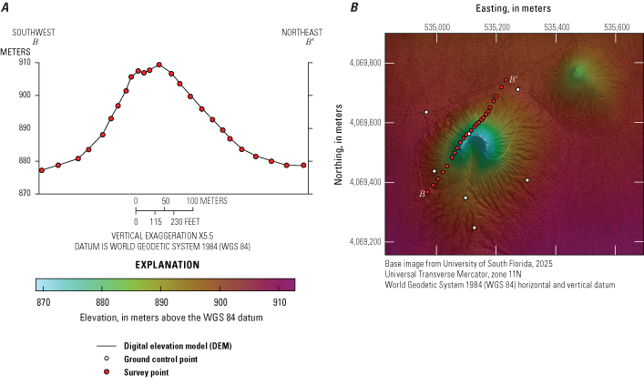
A, Extracted topographic profile from structure-from-motion (SfM) model along line of survey. B, Photogrammetry based digital elevation model (DEM) with Global Positioning System (GPS) survey points. DEM data are available in Van Alphen and others (2026).
Unoccupied Aerial Vehicle (UAV) Motor-Induced Noise Filtering
Following the methods described in Accomando and others (2021) and outlined here, a scalogram was produced to visualize the noise in the collected data before most of the data filtering, detrending, and so forth were performed (fig. 1.2). As in Accomando and others (2021), a large signal was observed at ~50 hertz, associated with the UAV’s motors.
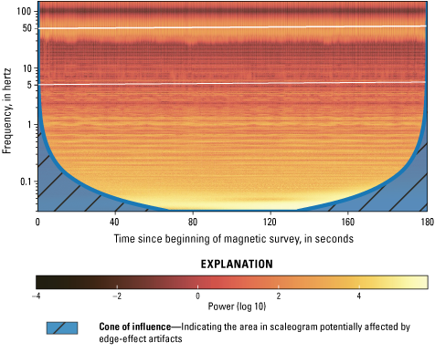
Scalogram of the observed unfiltered, untrended, ungridded magnetic data collected during 20 seconds of surveying. Strong signal at ~50 hertz shows the primary noise from unoccupied-aerial-vehicle motors.
Magnetic Base Station Cross-Correlation
The validity of using a remote base station to correct for the daily variation of the magnetic field was tested by calculating the cross-correlation of the observed total field between other stations at the same magnetic latitude. O’Neals, Calif. (FRN) was compared to the observed total field in Corbin, Va. (FRD), and to an even more remote station in Fürstenfeldbruck, Germany (FUR) (table 1.1). The maximum difference between the time-shifted total field observed at the different observatories is ~18 nanoTeslas (nT) for FRN-FUR, and ~10 nT for FRN-FRD (figure 1.3). The maximum correlation for FRN-FRD is 0.85 and 0.8 for FRN-FUR (table 1.2).
Table 1.1.
Locations of the geomagnetic observatories used for the cross-correlation.[IAGA, International Association of Geomagnetism and Aeronomy; IGRF, International Geomagnetic Reference Field; geomag., geomagnetic]
Location high resolution magnetic survey performed for this study: lat 36.77° N., long 116.61° W; quasi-dipole geomagnetic latitude of survey: lat 42.87° N.
Quasi-dipole latitude calculated using the calculator from British Geological Survey (2025).
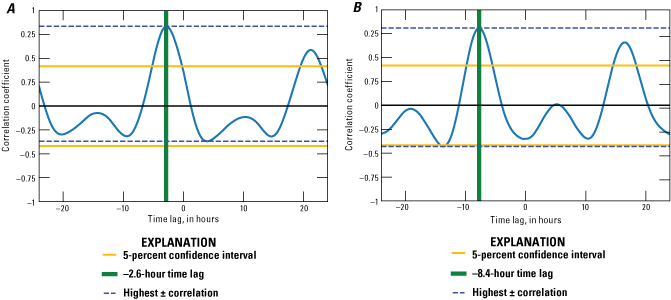
Graphs showing cross-correlation between the total observed field at observatories A, FRN and FRD, and B, FRN and FUR, October 18, 2019.
UAV Fencing
By using a UAV, it is easy to repeat the same survey lines at different survey altitudes above ground level. This fencing method provides an observed field that is a measurement of the upward continuation of the signal observed at the ground (or single flight altitude). These repeated flights along the same path allow us to observe the variation of the magnetic signal with altitude, both in terms of attenuation, and in terms of change in wavelength. Data were collected with consecutive flights above the same line at nine different altitudes from 20 to 100 meters (m) above ground level. Each line was approximately 1,400 m long, and the lines were flown in a north-south direction. Figure 1.4 represents the gridded data with vectors indicating the northern and vertical components of the observed field.
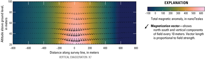
Graph showing gridded magnetic signal from “fencing” flights. Two-dimensional vector of magnetization shown with arrows representing the northern and vertical components of the field every 10 meters. The data are represented with respect to the average value of the magnetic field above the anomaly.
The ”fencing” dataset was used to verify the uncertainties introduced in the observed total field by altitude measurement errors. Using the field observed along a line at a particular altitude, it was possible to use an upward continuation filter (Henderson and Zietz, 1949; Dobrin and Savit, 1988) to compute the synthetic observation at a higher level. This value was then compared with the observed field measured at that altitude. The line at 40 m altitude was chosen and an upward continuation of 60 m (that is, taking it to 100 m) was performed. Comparing this line to the actual measured line flown at 100 m altitude, the upwardly continued line was observed to be ~20 nT lower than the value of the flown flight line (fig. 1.5). This difference indicates that the actual flight altitude difference should be less than 60 m. Varying the height of the upward continuation, the observed and the calculated lines overlapped at 56 m of altitude difference (fig. 1.6). This result indicates that for this pair of lines, the uncertainties associated with the flight altitude measurements are ~4 m, which corresponds to uncertainties of approximately 20 nT in the measured field. As indicated in 1.5A, the upward continuation filter performs well at the center of the flight line but not at the two ends.
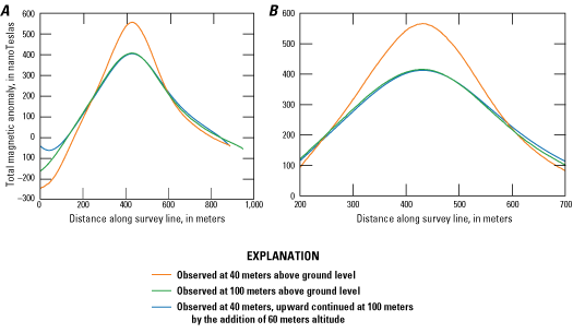
A. Comparison of the total field observed at the unoccupied-aerial-vehicle-measured altitudes of 40 and 100 meters (m) above ground level, with the upward continuation of the 40-m curve elevated by 60 m. B, Zoomed-in central part of panel A.
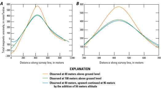
Best-fit upward continuation. A, Comparison of the total field observed at the unoccupied-aerial-vehicle-measured flight altitudes of 40 and 100 meters (m) above ground level, with the upward continuation of the 40-m curve elevated by 56 m. B, Zoomed-in central part of panel A.
Table 1.3 shows the difference in altitude required to achieve a good fit between the actual observed field at the higher altitude and the upwardly continued version of the lower flight line. The average difference in altitude between the UAV-flown flight altitude and its best-fit upwardly continued equivalent is 2.5 m, with a standard deviation of 4 m.
Table 1.3.
Difference in altitude between the upper flight altitude measured by the unoccupied aerial vehicles and the altitude of the best-fit upwardly continued lower line.[Every pair combination is listed here. All measurements in meters. All flight altitudes are above ground level.]
Notably, this fencing method not only provides a way to check the uncertainties associated with the flight altitudes, but it also provides the real field at different altitudes without the need to perform an upward continuation calculation. Furthermore, it also provides a downward continuation of the field, an operation that, in general, is not feasible using a mathematical formulation because it introduces noise that is often too large to be of any practical use. The fencing data collection also provides a measurement of the field at different altitudes along the full lateral extent of the flight line, whereas the mathematical formulation is accurate only in the central part of the flight line (as shown by the “tail” in the first ~100 m of the upward continued at 100 meters line in figs. 1.5, 1.6). The fencing method provides a full measurement of the three components of the magnetic field, including the rotation of the vector, which is not easily performed with mathematical filtering.
The ability to measure the full magnetic field at varying altitudes along an entire line provides additional data to constrain model inversions and offers insight that can be invaluable when differentiating between sources at different depths, or when performing topographic corrections to the observed data when magnetic material is present at the surface (for example, in an exposed lava flow).
References Cited
Accomando, F., Vitale, A., Bonfante, A., Buonanno, M., and Florio, G., 2021, Performance of two different flight configurations for drone-borne magnetic data: Sensors, v. 21, no. 17, article 5736, accessed February 2025 at https://doi.org/10.3390/S21175736.
British Geological Survey, 2025, Geomagnetic coordinate calculator: British Geological Survey website accessed February 2021 at https://geomag.bgs.ac.uk/data_service/models_compass/coord_calc.html.
Henderson, R.G., and Zietz, I., 1949, The upward continuation of anomalies in total magnetic intensity fields: Geophysics, v. 14, no. 4, p. 517–534, accessed May 2025 at https://doi.org/10.1190/1.1437560.
Van Alphen, R., Malservisi, R., Rodgers, M., and Connor, C., 2026, Data and codes utilized for the study of the lava flow of Little Cones, Nevada, USA, using UAV magnetic data (ver. 1): University of South Florida digital commons, https://doi.org/10.17632/zdcsk3rz9z.1.
Conversion Factors
International System of Units to U.S. customary units
Datums
Vertical coordinate information is referenced to the World Geodetic System of 1984 (WGS 84).
Horizontal coordinate information is referenced WGS 84.
Elevation, as used in this report, refers to distance above the vertical datum.
Altitude, as used for survey flights in this report, refers to height above local ground level.
Moffett Field Publishing Service Center
Manuscript approved for publication April 13, 2026
Edited by Mike Deacon
Illustration support by Kimber Petersen
Disclaimers
Any use of trade, firm, or product names is for descriptive purposes only and does not imply endorsement by the U.S. Government.
Although this information product, for the most part, is in the public domain, it also may contain copyrighted materials as noted in the text. Permission to reproduce copyrighted items must be secured from the copyright owner.
Suggested Citation
Van Alphen, R., Rodgers, M., Malservisi, R., Connor, C.B., Bakowski, R., and Berkey, T., 2026, High-resolution magnetic survey using an unoccupied aerial vehicle to constrain buried lava flow geometry, volume, and eruptive history of Little Cones, Crater Flat, Nevada, chap. R of Poland, M.P., Ort, M.H., Stovall, W.K., Vaughan, R.G., Connor, C.B., and Rumpf, M.E., eds., Distributed volcanism—Characteristics, processes, and hazards: U.S. Geological Survey Professional Paper 1890, 28 p., https://doi.org/10.3133/pp1890R.
ISSN: 2330-7102 (online)
Study Area
| Publication type | Report |
|---|---|
| Publication Subtype | USGS Numbered Series |
| Title | High-resolution magnetic survey using an unoccupied aerial vehicle to constrain buried lava flow geometry, volume, and eruptive history of Little Cones, Crater Flat, Nevada |
| Series title | Professional Paper |
| Series number | 1890 |
| Chapter | R |
| DOI | 10.3133/pp1890R |
| Publication Date | June 05, 2026 |
| Year Published | 2026 |
| Language | English |
| Publisher | U.S. Geological Survey |
| Publisher location | Reston, VA |
| Contributing office(s) | Volcano Science Center |
| Description | Report: vii, 28 p.; Data Release |
| Country | United States |
| State | Nevada |
| Other Geospatial | Crater Flat |
| Online Only (Y/N) | Y |
| Additional Online Files (Y/N) | N |