

Prospectivity Mapping for Geologic Hydrogen
Links
- Document: Report (23.4 MB pdf) , HTML , XML
- Related Work: Interactive web application for geologic hydrogen
- Data Release: USGS data release - Data Release for Prospectivity Mapping for Geologic Hydrogen
- Version History: Version History (8.00 KB pdf)
- NGMDB Index Page: National Geologic Map Database Index Page (html)
- Download citation as: RIS | Dublin Core
Abstract
Geologic, or naturally occurring, hydrogen has the potential to become a new, low-carbon, primary energy resource. Often referred to as “white” or “gold” hydrogen, this gas occurs naturally in the Earth’s subsurface, similar to petroleum resources. However, unlike petroleum, which releases carbon dioxide when burned, burning hydrogen only produces water as a byproduct. Exploration for geologic hydrogen remains in an early stage and discoveries of high concentrations of subsurface hydrogen are still relatively rare. To facilitate research and exploration for this potential resource, this report presents the first publicly available prospectivity map of geologic hydrogen accumulations in the conterminous United States. Prospective regions are those regions in which all major components necessary for a hydrogen accumulation likely are present—a source of sufficient hydrogen generation, porous reservoirs for storage, and seals to prevent leakage. The midcontinent region of the United States and the central California coast are revealed as having high prospectivity. This analysis also identifies previously unrecognized prospective regions that may be favorable due to long distance lateral migration of subsurface hydrogen, such as the offshore eastern seaboard of the United States, and can provide a linkage between surface observations of hydrogen degassing and far-field source regions. The methodology developed to create this map is expandable and flexible and may be adapted to incorporate new concepts in the hydrogen system and for application to other regions of the world.
Introduction
Hydrogen is ubiquitous at the Earth’s surface, and locally high surface fluxes of hydrogen have been known for decades, particularly at midocean ridges (Zgonnik, 2020). However, the potential for substantial subsurface hydrogen resources has been dismissed because hydrogen is highly reactive and diffusive (Apps and van der Kamp, 1993). Recent modeling has challenged this assumption, suggesting that thousands to billions of megatons of hydrogen may reside in the subsurface (Ellis and Gelman, 2024). Although much of this hydrogen likely is inaccessible because it is too deep, too far offshore, or in small accumulations that are not economically viable, even a small fraction could fill a substantial portion of the projected hydrogen demand in the coming years (Ellis and Gelman, 2024).
Until recently, subsurface hydrogen discoveries were generally unintentional and most likely went unreported because drilling mud gas logging tools do not routinely measure hydrogen, and hydrogen commonly is used as a carrier gas in laboratory gas analyses, preventing analysis of natural concentrations. In a world that historically has sought petroleum, discoveries of hydrogen-saturated formation fluids, if recognized at all, were generally considered a failure, and were ultimately abandoned. Therefore, despite the millions of exploratory and production boreholes that have been drilled throughout the United States (app. 1, fig. 1.1), the possibility of hydrogen as a new potential fluid target remains.
Recent discoveries of hydrogen across the globe include the Bourakebougou field in Mali (Prinzhofer and others, 2018; Maiga and others, 2023,56 2024) and in the Yorke Peninsula in South Australia (Boreham and others, 2021), as well as isolated but high concentrations observed in North America; other parts of Africa, Europe, Asia; and other parts of Australia (Zgonnik [2020] and references therein). Hydrogen also has been associated with subsurface helium discoveries (Milkov, 2022). Within the United States, hydrogen has recently been reported in Arizona, California, Kansas, Montana and Nebraska (U.S. Geological Survey [USGS], 2019; Zgonnik, 2020). Observations of hydrogen in concentrations of more than 0.5 mole percent (mol%) are shown in figure 1, illustrating a general scattering of hydrogen occurrences throughout the United States (USGS, 2019; Zgonnik, 2020; Brennan and others, 202113). Particularly high concentrations have been found in the midcontinent region, around the Four Corners area (Arizona, Colorado, New Mexico, and Utah), and along the coast of California. However, little has been published on establishing the controls on the locations of these occurrences and thus, predictability remains low.

Map showing concentrations of geologic hydrogen greater than 0.5 mole percent as reported in drill-well gas samples throughout the conterminous United States (data from U.S. Geological Survey [2019], Zgonnik [2020], and Brennan and others [2021]). Symbol size correlates with concentration. Labeled concentrations are rounded to the nearest integer value.
To facilitate continued exploration of this new potential energy resource, research into ways to identify regions that may be favorable for hydrogen exploration is underway. In 2021, Boreham and others (2021) published a radiolytic production rate map for Australia, delivering the first regional-scale map depicting relative favorability for hydrogen throughout that country. However, that map relied heavily on surface geology extrapolated to a depth of one kilometer (km), which may be of limited utility due to lithologic heterogeneity along such distances, and the map did not fully integrate the spatial distribution of hydrogen generation sources with other potential factors, such as reservoir or seal potential. In particular, the use of geophysical potential fields data may provide an understanding of geology at depths greater than 1 km. Considering several additional sources of hydrogen generation and integrating a variety of surface and subsurface datasets, this report presents the first publicly available map of geologic hydrogen prospectivity for the conterminous United States.
Purpose and Scope
Geologic evaluations of subsurface resources are initiated on broad spatial scales that narrow with increasing knowledge. Studies begin with regional or “play” assessments that serve to prioritize areas for future, more focused efforts (Lottaroli and others, 2018). Because geologic hydrogen is a resource recently discovered, our methodology is designed for the regional—or even continental—scale, and our purpose is to identify areas of the conterminous United States for more indepth research.
In defining the geologic hydrogen system and the components necessary for potential accumulations to exist, this report distinguishes between the “play” scale and the “prospect” scale. At the play scale, we do not try to define where or at what depth specific hydrogen accumulations may exist, but instead, focus on the spatial layering of processes that are required for accumulations to occur generally. Processes such as the generation of geologic hydrogen, its broad migration direction, reservoir porosity for its storage, and seal capacity for prevention of leakage to the surface are tractable to evaluate at regional scales. Processes that define or are related to localized prospects may include subsurface traps; reservoir temperature; biotic or abiotic consumption; or the detailed migration, mixing, and phase behavior with other fluids (water, hydrocarbon, nitrogen, and so on). Although these latter processes are also relevant and important at the play scale, they are difficult to map accurately on broad spatial scales and thus we have not incorporated them into our 2024 methodology. Future work may address this difficulty as it becomes more feasible and as more is learned about the subsurface hydrogen system.
Hydrogen System Components
For purposes of this report, the geologic hydrogen system at the continental scale is defined as comprising three primary components: source, reservoir, and seal. Future work may add a fourth component addressing the preservation of hydrogen, because it is highly reactive. The source component is defined by the mechanism for the generation of geologic hydrogen and incorporates possible vertical and lateral fluid migration. The reservoir component is defined by the presence of porosity in the subsurface to store hydrogen. The seal component is defined by the presence of low-permeability rocks paired with potential reservoirs to prevent seepage and loss of hydrogen to the surface.
The source component of the hydrogen system has received the most attention in previous studies and several potential mechanisms have been proposed for the presence of hydrogen in the mid-to-upper crust (Sherwood Lollar and others, 2014). For example, serpentinization, or the oxidation of iron in the presence of water, is the main source of hydrogen in midocean ridge settings (Frost and Beard, 2007; Liu and others, 2023), in subduction zones within the mantle wedge or slab itself (Guillot and others, 2001), and may occur when ultramafic rocks are in contact with water at moderately high temperature (200–315 degrees Celsius [°C]; McCollom and Bach, 2009). The radiolysis, or molecular splitting of groundwater through contact with radiogenic rocks, is another commonly cited source of hydrogen. Helium is also generated by decay of radiogenic nuclides in similar rocks and may be colocated with hydrogen; figure 1.2 in appendix 1 shows the subsurface helium distribution in the conterminous United States. Radiolysis, however, tends to rely on potassium-thorium-uranium series decay from crystalline, granitoid-type rocks and, therefore, requires long residence times (hundreds of millions to billions of years) for an effective volume of hydrogen generation. Some authors have also proposed that hydrogen is generated from overmature, organic-rich rocks (Horsfield and others, 2022; Mahlstedt and others, 2022; Boreham and others, 2023; Hanson and Hanson, 2024), although this hypothesis remains difficult to represent on broad spatial scales because of a lack of sampling of very high maturity rocks since they have limited utility for hydrocarbon exploration. Alternatively, hydrogen is likely to be consumed by lower-maturity, organic-rich rocks during thermal maturation and petroleum generation (Apps and van der Kamp, 1993; Smith and others, 2005) or adsorbed in some clay minerals that may be present in fine-grained mudrocks (Wang and others, 2023). In both cases, the depths of organic-rich rocks become critically important (optimal conditions require great depths for hydrogen generation and shallow depths for hydrogen consumption) and may be addressed more tractably at basin or subregional spatial scales. Poorly defined deep sources of hydrogen may exist from the primordial Earth formation, with slow degassing during Earth’s history, or may consist of hydrogen of indeterminate origin that has migrated through the lithosphere to mid- or upper-crustal levels along deep crustal-scale faults (Zgonnik, 2020).
As a first approach, we have simplified the source subcomponent mechanisms to include the following:
• Serpentinization-type reactions based on the identification of ultramafic rocks but without consideration of water or temperature ranges;
• Radiolysis of water based on the identification of Archean or Proterozoic granitoids, without consideration of the presence of water; and
• Deep sources of hydrogen.
The details of these modeled subcomponents are provided in the “Methods” section of this report. Additionally, buoyant migration of subsurface fluids allows for the transportation of hydrogen from source to reservoir and allows a broad footprint of reservoirs to access hydrogen that is generated downdip. Long-distance lateral migration is well established in petroleum systems (Tissot and Welte, 1984; Hunt, 199640). Here, we use a similar approach to model the migration pathways that may be expected from hydrogen source rocks, which realistically expands the spatial reach of these source rocks and incorporates lateral migration into the source subcomponents.
Reservoir and seal components are likely to be broadly comparable to those components of hydrocarbon and other subsurface natural gases. Because the diffusivity of hydrogen is similar to that of helium (Jacops and others, 2017), hydrogen may be sealed by similar rock facies and in similar trapping configurations. Because most helium and hydrocarbon gases are in sedimentary reservoirs with sedimentary seals, the presence of sedimentary strata is given preference as a first proxy for the presence of reservoir and adequate sealing facies. Lateral and vertical migration of hydrogen from source rocks (some of which may be quite deep, for example, serpentinization sources) is also modeled using methodologies developed for other subsurface gases where long distance migration is well-established (Tissot and Welte, 1984; Hunt, 1996).
Methods
The spatial distributions of hydrogen system components are integrated based on presence to identify highly prospective regions. However, because there is uncertainty in the presence of these components in the subsurface, a chance of sufficiency (COS) methodology was selected to establish fractional probabilities of each component’s presence and effectiveness, which is explained in more detail in the “Assigning Chances of Sufficiency” and “Risk Analysis” sections of this report. “Sufficiency” is defined as the viability of a hydrogen system component to contribute to a subsurface occurrence of hydrogen. Because no volumes are known yet for subsurface hydrogen occurrences, this definition is not benchmarked to any specific volume. The minimum concentration for an occurrence is 0.5 mole percent (mol%; fig. 1). The COS similarly does not imply a statistical likelihood of subsurface hydrogen being found. For example, a source COS of 0.5 does not imply that 50 percent of wells in a particular location will successfully observe hydrogen or even a hydrogen source. Rather, this COS metric is used in this early exploratory stage to establish a relative scale on which to evaluate prospectivity from one location to another, based on the stacking of hydrogen system components. Similar knowledge-based quantitative probability methods have been used in petroleum evaluations (White, 1993; Otis and Schneidermann, 1997), geothermal studies (Ito and others, 2017), seabed mineral deposit studies (Juliani and Ellefmo, 2019), and even subsurface radioactive waste disposal studies (Malvić and others, 2020).
The hydrogen prospectivity map of the conterminous United States integrates 21 layers of geological and geophysical data. Table 1 outlines the 3 primary model components, the 3 source subcomponents, the 21 individual layers, the distribution of the COS assigned to each layer, the spatial buffers applied, and the layers that incorporate lateral migration—all of which inform the geologic hydrogen model. Raster grids for each of these layers are provided in the associated USGS data release (Hearon, 2025). The COS for each layer is assigned based on interpretations of the geologic hydrogen model and broad knowledge of the geology of the conterminous United States.
Table 1.
Primary components, input layers, and risk analysis summary of the geologic hydrogen model.[Low, mid, and high values for chance of sufficiency (COS) are used to quantify subcomponent uncertainty ranges during the stochastic uncertainty analysis part of the modeling. The methodology for lateral migration is explained in detail in the “Lateral Migration of Subsurface Fluids” section of this report. SP, serpentinization; km, kilometer; RD, radiolysis; DP, deep; mW/m2, milliwatt per square meter; ±, plus or minus; RS, reservoir; SL, seal]
Serpentinization as a Hydrogen Source
Reduction of water by oxidation of iron-containing minerals in ultramafic rocks (that is, serpentinization-type reactions) is one of the most widely cited mechanisms for the formation of natural hydrogen (Gaucher, 2020; Zgonnik, 2020; Blay-Roger and others, 20248). The modeled serpentinization subcomponent (SP) comprises five layers (SP1 to SP5) predicated on the presence of subsurface ultramafic rocks (fig. 2). Layer SP1 is the area defined by the east coast magnetic anomaly (ECMA), which is expressed as an offshore, high-amplitude, positive magnetic anomaly extending from the coast of Georgia to the coast of Nova Scotia. Previous studies suggest that the anomaly may be caused by the presence of subsurface ultramafic rocks or serpentinized mantle material associated with the boundary between rifted continental and oceanic crust (McBride and Nelson, 1988; Wu and others, 2006; Biari and others, 2017). Layer SP2 is defined by areas where ultramafic rocks are present at the surface (Krevor and others, 2009; Faure, 2010; Horton and others, 2017) and are inferred to potentially extend into the subsurface. This layer includes broad coverage of ultramafic rocks, including banded iron formations, which have been proposed as additional hydrogen source rocks beyond traditional peridotitic lithologies (Geymond and others, 2022, 2023). Layer SP3 contains areas that are underlain by the midcontinent rift, the southern Oklahoma aulacogen, and the Reelfoot rift (Elling and others, 2022). These areas represent three failed Proterozoic midcontinental rifts that are defined by prominent, high Bouguer gravity anomalies. Rift settings are known for isostatic shallowing of the crust-mantle boundary, promoting the presence of shallow ultramafic rocks and commonly featuring exhumed mantle (McKenzie, 1978; Boillot and others, 1980; Manatschal, 2004; Gillard and others, 2019).
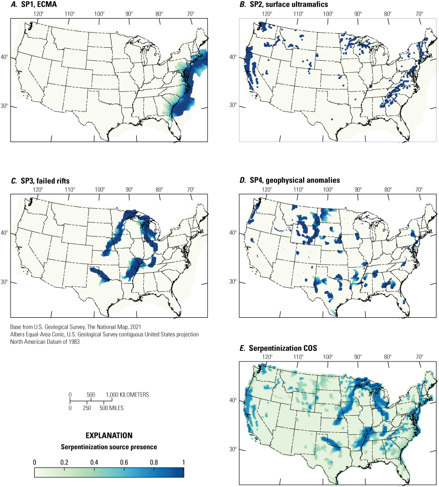
Maps showing the presence of serpentinization subcomponent (SP) source layers SP1–SP4 from table 1 and the chance of sufficiency (COS) for the composite serpentinization source subcomponent. A, SP1 shows the location of and migration pathways from the east coast magnetic anomaly (ECMA). B, SP2 shows the location of surficial ultramafic rocks with a 20-kilometer buffer. C, SP3 shows the location of and migration pathways from three failed rifts. D, SP4 shows the location of and migration from geophysical anomalies. E, The final, deterministic serpentinization source subcomponent COS.
Layer SP4 outlines subsurface regions that may contain ultramafic rocks based on geophysical potential fields data. Isostatic gravity data (Kucks, 1999) and magnetic data (Bankey and others, 2002) were considered where overlapping positive anomalies in both datasets were initially hypothesized to indicate the presence of potentially serpentinized, dense ultramafic rocks at depth. Because potential fields signals can be generated by numerous nonunique sources, this filter is being used to target dense and magnetic rocks in general, which can include serpentinites (which may be lower density than their unserpentinized precursors, but still are dense relative to granitoids and most sedimentary rocks) as well as banded iron formations. To better identify sources at midcrustal depths, the magnetic data are a 500 km high-pass filtered dataset (Bankey and others, 2002), which removes long wavelengths. Two magnetic maps were then generated: (1) a reduced-to-pole dataset and (2) a dataset with a pseudogravity transformation (Blakely, 1995; Oakey and Saltus, 2016). The latter was created to better highlight magnetic source bodies and provide a more comparable wavelength spectrum to the gravity data. Two index maps were created to display gravity and magnetic data using both datasets (fig. 3) and were used to highlight regions with positive gravity and positive magnetic signatures which may indicate greater potential for subsurface ultramafic lithologies. The regions from layer SP3 (failed rifts) were used to check for expected positive gravity-magnetic signatures but were observed to contain positive gravity, but mixed magnetic anomalies. This observation aligns with that of Bonnemains and others (2016) in which the magnetic signatures of serpentinized ophiolites can depend on the temperature and thus mineralogy of the serpentinization reaction, as well as the degree of serpentinization. Given the ambiguous magnetic signature of serpentinites, only isostatic gravity was ultimately considered in the model for layer SP4. Furthermore, although Laramide-associated basement uplifts (for example, the Wind River Range, Bighorn Mountains, Laramie Mountains, and Granite Mountains in Wyoming, and Black Hills in South Dakota and Wyoming) display strong, positive isostatic gravity anomalies, these mountains were expected to be predominantly felsic, yet remain in the model results; we note that rare ultramafic rocks have been observed in these ranges (Potts, 1972; Manzer and Heimlich, 1974; Harper, 1986), and hypothesize that more may exist at depth, accounting for the strong positive gravity anomaly. The midcontinent rift, southern Oklahoma aulacogen, and Reelfoot rift defined in SP3 were then removed from layer SP4 so that they are not represented twice in this analysis.

Magnetic and gravity maps to identify subsurface ultramafic rocks. Isostatic gravity (data from Kucks [1999]) and magnetic (data from Bankey and others [2002]) maps were combined into index maps to identify regions with overlapping positive (+) and negative (−) gravity and magnetic signatures. Dark brown regions indicate areas with positive gravity and positive magnetic signatures, whereas light green regions indicate areas with positive gravity but negative magnetic signatures. A, Index map using a high pass (500 kilometers) reduced-to-pole (RTP) magnetic dataset (Bankey and others, 2002). B, Index map using a pseudogravity approach to the magnetic data. In A and B, the index map indicates signs of both potential fields data, where positive gravity and positive magnetics were initially hypothesized to indicate potential ultramafic subsurface bodies. Ultimately, a mixed magnetic signature is instead observed in failed rift regions where ultramafic rocks are more likely to occur in the subsurface. Therefore, only gravity data were used in the final model for serpentinization subcomponent (SP) source layer SP4. The outline of the failed rifts (Elling and others, 2022) is shown in black for reference.
Finally, layer SP5 represents potential serpentinization sources throughout the entire United States that are unknown and have not been explicitly accounted for in layers SP1–SP4. Thus, this layer is given an evenly applied nonzero COS across the Nation.
Radiolysis as a Hydrogen Source
Along with serpentinization, radiolysis of water by ancient, radiogenic rocks also is commonly considered a major source of geologic hydrogen (Sherwood Lollar and others, 2014; Gaucher, 2020; Zgonnik, 2020). The modeled radiolysis subcomponent (RD) is split into five layers (RD1 to RD5) that represent the presence of radiogenic subsurface rocks (fig. 4). Layer RD1 contains areas with known subsurface uranium deposits and RD2 displays areas that are favorable for the concentration of uranium in the subsurface. These layers were compiled by the USGS from published sources and are available from the U.S. Energy Information Administration (U.S. Energy Information Administration, 2020a, b91). Because uranium decay can cause the radiolysis of water, both layers were used but have different COS values.

Maps showing the presence of radiolysis subcomponent (RD) source layers RD1–RD5 from table 1 and the composite chance of sufficiency (COS) for the radiolysis subcomponent source layer. A, RD1 shows the location of and migration pathways from known uranium deposits with a 10-kilometer (km) buffer. B, RD2 shows the location of and migration pathways from the areas favorable for uranium with a 10-km buffer. C, RD3 shows the location of the Precambrian craton with a 100-km buffer. D, RD4 shows the location of accreted terranes with a 100-km buffer. E, RD5 shows the location of young, Phanerozoic granitoids with a 20-km buffer. F, Map showing the composite radiolysis COS source subcomponent.
Layer RD3 covers regions that are underlain by the Archean and Proterozoic cratonic platform (Marshak and others, 2016). The granites and granitoids of the North American craton are commonly enriched in radioactive elements such as uranium and thorium and are sufficiently old to allow for abundant decay of these long-lived radionuclides. Layer RD4 contains geologically younger regions that are not underlain by the craton and thus is an inverse layer from RD3. The area outlined in RD4 is underlain by terranes of the western and eastern North American cordillera as well as the southeastern coastal plain that were accreted throughout the Phanerozoic (Marshak and others, 2016). These rocks are highly variable in lithology and age and, therefore, also highly variable in the concentration of radioactive elements and time for decay. Thus, a lower COS is assigned to RD4 regions relative to those regions in RD3.
Finally, layer RD5 represents areas with Phanerozoic granites and granitoids (Horton and others, 2017). These rocks are common along the western cordillera of the United States, and may be enriched in uranium and thorium, but have not had the long residence time needed for abundant radioactive decay.
Deep Sources of Hydrogen
The deep-sourced subcomponent captures a potential supply of geologic hydrogen that is derived from sources in the lower crust, or possibly deeper in the Earth’s interior. The exact generation mechanism for this inferred source is not known but may be the decomposition or dehydration melting of dense, hydrous silicate phases introduced by subducted slabs to the deep mantle (Williams and Hemley, 2001; Hirschmann, 2006; Ohira and others, 2014) or the outgassing of primordial hydrogen from the core and mantle (Williams and Hemley, 2001; Loewen and others, 2019; Olson and Sharp, 2022). The deep source subcomponent (DP) is split into four layers (DP1 to DP4; fig. 5). Layer DP1 includes areas of mapped, kilometer-depth scale surface faults (McCafferty and others, 2023). Faults can connect to and provide pathways for geologic hydrogen to migrate from lower crustal sources into reservoirs for storage. Layer DP2 consists of areas of Proterozoic suture zones (Whitmeyer and Karlstrom, 2007). These areas are interpreted to represent significant internal lithospheric boundaries that may promote fluid migration from depth. Phanerozoic suture zones, such as the Coast Range, San Andreas Fault, the various Appalachian and Ouachita belts, and the Suwannee suture zone (among others) may also represent similar lithospheric boundaries. These areas were not included in initial mapping because of the lack of a unified data layer; however, these areas can be incorporated into this workflow when available. Layer DP3 captures regions of high heat flow (Blackwell and others, 2011), defined here as greater than 80±10 milliwatts per square meter (mW/m2). These high heat flow regions are commonly associated with geothermal fluid circulation and may promote hydrogen migration from depth. Volcanic fluids and geothermal springs have been observed to contain hydrogen as well as hydrogen-metabolizing organisms (Spear and others, 2005; Lindsay and others, 2019; Zgonnik, 2020). Lastly, layer DP4 represents potential deep sources of hydrogen throughout the United States that are unknown and have not been explicitly accounted for in layers DP1, DP2, and DP3. Similar to SP5, DP4 is given an evenly applied, nonzero COS across the United States.
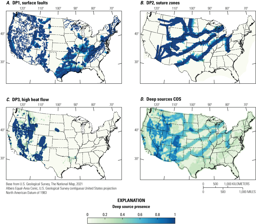
Maps showing the presence of deep source subcomponent (DP) source layers DP1–DP3 from table 1 and the composite chance of sufficiency (COS) for the deep sources subcomponent. A, DP1 shows the location of and migration pathways from surface faults with a 10-kilometer (km) buffer. B, DP2 shows the location of and migration pathways from suture zones with a 40-km buffer. C, DP3 shows areas of high heat flow (defined here as 80 milliwatts per square meter [mW/m2] with a ±10 mW/m2 buffer. D, Map showing the composite COS for the DP subcomponent.
Lateral Migration of Subsurface Fluids
Migration of subsurface fluids is governed by porosity and permeability pathways within and between rock units, including permeability induced by naturally occurring fractures and faults. Furthermore, in multiphase immiscible fluid systems (such as hydrocarbon and water or a hydrogen gaseous phase and hydrogen-saturated water), buoyancy forces also drive migration. These processes are complex and can occur in both sedimentary settings, as has been shown abundantly in petroleum systems (Tissot and Welte, 1984; Hunt, 199640), as well as in metamorphic and igneous rocks, as has been demonstrated primarily in geothermal applications (Ingebritsen and Manning, 2010; Lamur and others, 2017). The direction of fluid flow also is complex (Bjorlykke, 2010), and a detailed examination is beyond the scope of this preliminary favorability mapping study. To determine favorable areas for possible hydrogen accumulations, we focus on the flow directions associated with the long-distance lateral migration that commonly occurs in sedimentary basins. For this report, this long-distance lateral migration is defined as migration across map distances of up to 250 km. Simple methods for mapping lateral fluid flow are well established from petroleum and hydrologic studies and include drainage area delineation (Hubbert, 1953) and flow line mapping (Tóth, 1962), both of which are used for this report.
To provide a single migration surface for modeling lateral hydrogen migration in sedimentary settings throughout the United States, an elevation map of basement rocks was created. This surface is defined as the base of the stratigraphic section in regions with sedimentary surface geology and is otherwise coincident with topography in regions with metamorphic or igneous surface geology. The map was created by subtracting the total thickness of sedimentary rocks (Frezon and others, 1983) from the GEBCO 2023 digital elevation model (GEBCO Bathymetric Compilation Group, 2024). Because lateral migration was only modeled in sedimentary settings for this study, regions that have metamorphic or igneous rocks cropping out were ultimately removed from the map. The resultant basement elevation surface is shown in figure 6.
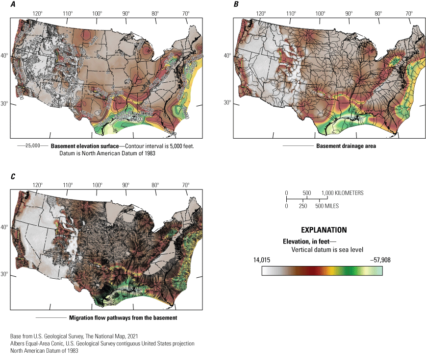
Basement structure map and hydrogen migration flow lines. Maps showing A, the basement elevation surface in feet; B, basement drainage areas; and C, migration flow pathways from the basement. A higher resolution version of part C is available in figure 1.3 in appendix 1.
Map-based migration analysis began with the delineation of drainage areas and was followed by the creation of flow lines in all areas with sedimentary cover (fig. 6). The migration pathways were created with SLB PetroMod version 2020.1 (SLB, 2020), using the PetroCharge Express tool, and were modeled on the basement elevation surface described in the preceding paragraph; a high-resolution version of these flow lines is shown in fig. 1.3 in appendix 1. During lateral migration, hydrogen is assumed to be a separate phase that is buoyant relative to groundwater and is consumed biotically and abiotically (Gregory and others, 2019); this consumption is accounted for in the model by linearly decreasing the COS as lateral migration distance increases from 0 to 250 km from the source.
For each source layer that explicitly represents a subsurface source (identified in table 1 as “Lateral migration”), the following workflow was developed:
-
1. Source presence defined by the layer is clipped to only include source in areas with sedimentary cover.
-
2. A spatial buffer was applied, as given in table 1, to provide coarser spatial resolution to point features.
-
3. A Matlab script (app. 2) was developed that first created a list of grid cells with source presence, and then:
-
4. A resulting pointset with migration distances for the layer was then interpolated using the ArcGIS Empirical Bayesian Kriging tool (Krivoruchko and Gribov, 2019) to provide a raster map of migration distance.
-
5. The migration distance grid was then converted to a COS grid by linearly interpolating between 0 and 250 km distances corresponding to a COS of 1 and 0, respectively.
-
6. Any migration distance beyond 250 km was given a COS of zero.
Reservoir and Seal
Although a source of hydrogen is critically important for determining where hydrogen may be flowing in the subsurface, a porous reservoir that is sealed by low permeability caprock is likely to be required for economic accumulations to be realized. This analysis treats reservoir and seal on a continental scale and, therefore, the main discriminator for predicting the potential for lithologies with sufficient reservoir quality is simply the presence or absence of sedimentary strata. Although fractured crystalline rock may be permeable as is demonstrated in geothermal applications (Lamur and others, 2017), or as has been observed in relatively rare petroleum accumulations (Petford and McCaffrey, 2003), the same geologic processes that led to those fractures likely preclude the existence of a competent seal.
The reservoir component (RS) focuses on the presence of predictable porosity and permeability and is composed of three layers (RS1 to RS3; fig. 7). Layer RS1 indicates the presence of sedimentary strata based on surface geology; layer RS2 is the inverse (Horton and others, 2017), indicating regions with metamorphic or igneous rocks at the surface and therefore likely an absence of sedimentary strata in the subsurface as well. The COS assigned to RS1 is higher than that assigned to RS2 (table 1), representing the higher likelihood of sufficient reservoir when sedimentary rocks are present. Finally, many regions of the United States have sedimentary rocks at the surface, but the overall sedimentary cover may be thin (less than a few kilometers), leading to a marginally lower likelihood of a viable hydrogen reservoir. Layer RS3, which highlights regions within well-defined sedimentary basins (Frezon and Finn, 1988), is included to capture the benefit of having a thick sedimentary column and, therefore, many potentially viable reservoirs available.
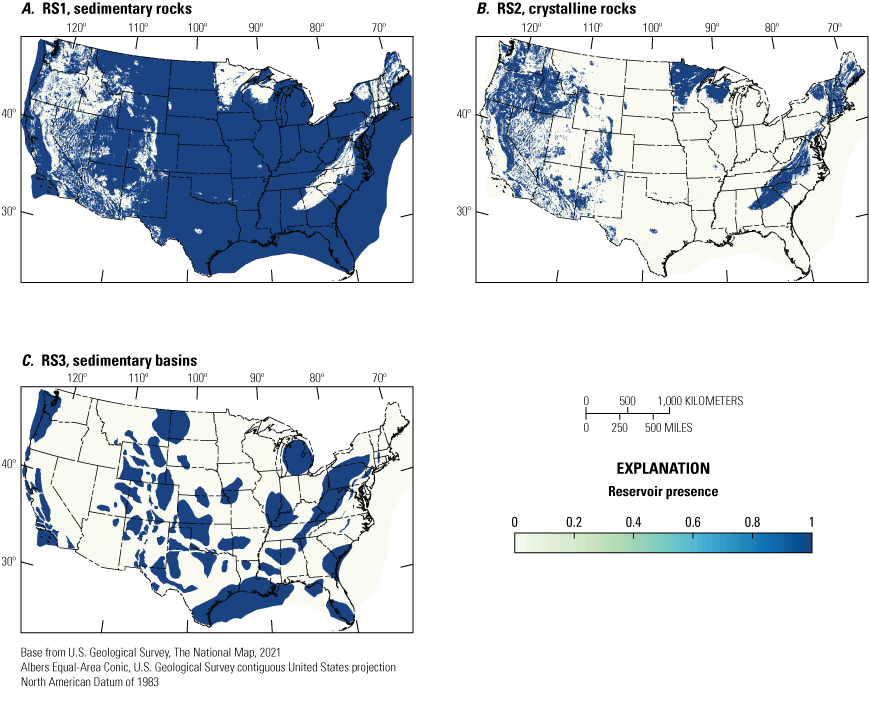
Maps showing the presence of reservoir component (RS) layers RS1–RS3 from table 1. A, RS1 shows the location of sedimentary rocks. B, RS2 shows the location of crystalline rocks. C, RS3 shows the location of sedimentary basins.
The seal component defines the presence of predictable, low-permeability rocks paired with reservoirs that can keep hydrogen in the subsurface and prevent seepage to the surface. This component is composed of four seal (SL) layers (SL1 to SL4; fig. 8). Layer SL1 defines the presence of evaporites in the subsurface (Ege, 1985) as salt layers provide notably good sealing facies (Beauheim and Roberts, 2002). Layers SL2, SL3, and SL4 are the same as the reservoir layers RS1, RS2, and RS3 because the presence or absence of sedimentary strata is taken as the primary driver for the possibility of a viable sealing facies in the subsurface. However, the COS values are lower when these layers were used in the seal component, reflecting an increased general sense of risk in seal over reservoir. Furthermore, thicker sedimentary strata associated with basins are interpreted to offer the benefit of (1) sufficient burial to compact rocks to low porosity and (2) a higher likelihood of one or more potential sealing formations throughout the stratigraphic column.
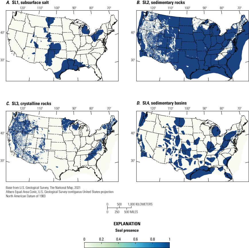
Maps showing the presence of potential seal component (SL) layers SL1–SL4 from table 1. A, SL1 shows the location of subsurface salt deposits. B, SL2 shows the location of sedimentary rocks. C, SL3 shows the location of crystalline rocks. D, SL4 shows the location of sedimentary basins.
Assigning Chances of Sufficiency
The COS values for each component and subcomponent were assigned using an expert elicitation, or expert-driven, approach using a peer review panel (O’Hagan and others, 2006). During this panel, the authors presented all data layers and gained feedback on the methods and COS confidence ranking between components and subcomponents. The panel audience was two geoscience subsurface data specialists, a geoscientist with extensive experience conducting petroleum assessments in the public sector, a geoscientist with extensive experience conducting petroleum play and prospect assessments in the private sector, and two geophysicists with extensive backgrounds in the public and private sectors using potential fields data.
The final COS values for each hydrogen system component are illustrated with an uncertainty matrix (fig. 9). Uncertainty matrices are widely used to represent the effect and uncertainty in a model parameter (Fugelli and Olsen, 2005; Speziale and Geneletti, 2014). As provided in table 1, subcomponent layers are assigned a median COS and an uncertainty range represented by high and low COS endmembers. To determine these values, the data layer is considered in terms of its sufficiency for the hydrogen system, as well as confidence that includes uncertainty in the input data layer itself and uncertainty in its sufficiency median value. Recommended COS values and ranges are shown in an uncertainty matrix format in figure 9A. The COS values in this matrix were obtained during an iterative process of balancing confidence in data layers with their importance for the hydrogen system. Model results are less sensitive to the absolute COS value and instead depend more on relative COS differences assigned to various model layers. Increasing knowledge of the hydrogen system may result in modifications to these preliminary COS values. Uncertainty ranges assigned in figure 9A generally indicate increasing (but symmetrical) ranges with decreasing confidence. The exception is the lowest left domain (low confidence, low sufficiency); this uncertainty range is only 0.1 to prevent negative numbers while maintaining symmetrical distributions. To illustrate the methodology, source subcomponent data layers are plotted in figure 9B. The reservoir and seal component layers followed the same methodology.
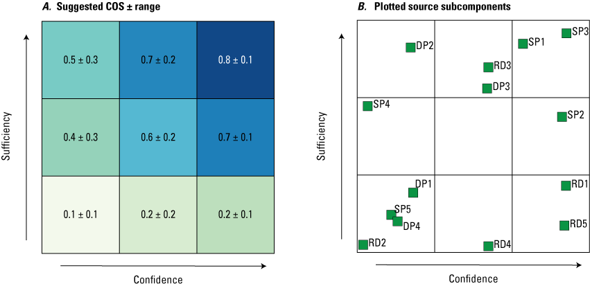
Graphs showing the chance of sufficiency (COS) for source subcomponents. An expert-driven approach was combined with a 3 by 3 uncertainty matrix to assign COS values to hydrogen system component and subcomponent layers. A, An uncertainty matrix provides consistent median and range values for COS. Increasing confidence corresponds with reduced or tighter COS ranges, whereas increasing sufficiency corresponds with increasing median COS. B, All source subcomponents plotted in the same uncertainty matrix format. Refer to table 1 for layer COS median and range values (high and low COS endmembers) used in the prospectivity model. ±, plus or minus; DP, deep sources of hydrogen subcomponent layer; RD, radiolysis subcomponent layer; SP, serpentinization subcomponent layer.
Risk Analysis
All three primary model components—source, reservoir, and seal—are required for a successful subsurface accumulation of geologic hydrogen. Mathematically, we quantified the likelihood of sufficiency of each of these primary components with a COS as described in the beginning of the “Methods” section of this report. The COS values for the primary model components are shown in table 1. The total hydrogen prospectivity, P, is then described by:
whereP
is the value for the total hydrogen prospectivity;
COS
is the chance of sufficiency;
SC
is the COS for the source components;
RS
is the COS for the reservoir component; and
SL
is the COS for the seal component.
Within each primary hydrogen system component, multiple layers have been considered that may contribute to the sufficiency of that component. We treat these using the following relations for each primary hydrogen system component:
whereSP
is the value for the source subcomponent of serpentinization;
RD
is the value for the source subcomponent of radiolysis; and
DP
is the value for the source subcomponent of deep sources.
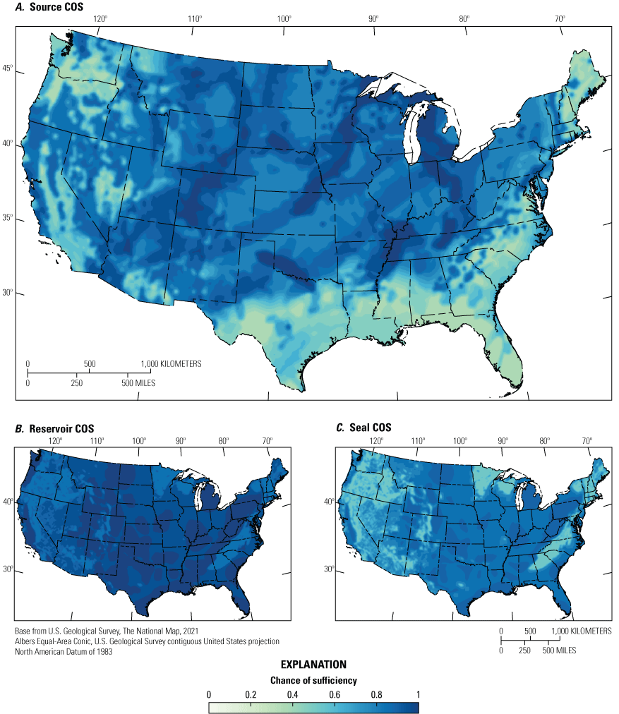
Maps showing the deterministic chance of sufficiency (COS) for the three primary hydrogen system components: source, reservoir, and seal. Composite source COS is drawn from three subcomponents: serpentinization, radiolysis, and deep sources of hydrogen. Quantitative integration of these subcomponents is described in the “Risk Analysis” subsection of the “Methods” section of this report. A, Source COS serves as an important map for hydrogen capture or stimulation resources, as reservoirs, traps, and seals are not required. B, Reservoir COS is based primarily on the occurrence of sedimentary rocks, which provide predictable porosity to store subsurface fluids. C, Seal COS is likewise based primarily on the occurrence of sedimentary rocks, which provide predictable low-permeability facies to prevent subsurface fluid leakage.
Finally, since each source subcomponent itself incorporates several layers, these are defined by:
where the subscripts in equations 5, 6, and 7 are described for each layer in the “Serpentinization as a Hydrogen Source,” “Radiolysis as a Hydrogen Source,” and “Deep Sources of Hydrogen” subsections of this report. The COS maps are shown for equation 5 (fig. 2E), equation 6 (fig. 4F), and equation 7 (fig. 5D).Equations 2–7 all incorporate multiple layers by multiplying chances of insufficiency, which is defined as 1–COS, rather than COS directly. The COS for each hydrogen system component or subcomponent is then recovered by subtracting the cumulative chance of insufficiency. This method allows multiple layers to contribute by increasing the COS where they spatially overlap, and unlike the primary components, not all layers must exist simultaneously for an accumulation to occur. Using this methodology, multiple overlapping layers results in only an incremental improvement in the overall component or subcomponent COS. For example, for the seal component in a region where sedimentary rocks are present, the additional presence of salt improves the overall COSRS from 0.8 to 0.82 (for the midcase COS values in table 1). Furthermore, if that region is within a well-defined sedimentary basin, the COSRS improves to 0.874.
All layers were mapped on an initial 1-km square grid; the final risk analysis was performed on a slightly coarser 5-km square grid. A Matlab script to solve equations 1–7 is provided in appendix 2. Equations 1–7 can also be easily solved using raster calculators in geographic information systems (GIS) software.
Uncertainty Quantification
Although the COS assigned to each layer represents a quantification of a likelihood or probability of sufficiency, these values remain uncertain. To quantify the range of uncertainty in each layer, we used a stochastic Monte Carlo approach to our modeling. Table 1 provides the low, mid, and high COS values for each layer, which were used to create triangular distributions for sampling during the probabilistic simulation (sampling distributions are shown in figs. 1.4 and 1.5). Triangular distributions were assigned because low and high values were intended to represent the bounds of acceptable values but were less likely than mid COS values. A total of 5,000 simulations solving equations 1–7 were then calculated, and resultant maps were created displaying the exceedance probability for 10 percent (P10), 50 percent (P50), and 90 percent (P90) values for the COS of the serpentinization (fig. 1.6), radiolysis (fig. 1.7), and deep sources (fig. 1.8) subcomponents; for the primary source (fig. 1.9), reservoir (fig. 1.10), and seal (fig. 1.11) components; and the final prospectivity (fig 1.12).
Compiled Observational Data Sources
Several sources of observed data were compiled to support this study. These sources include a map showing the distribution of previously drilled oil and gas wells from Skinner and others (2022), which helps illustrate where the subsurface has or has not been extensively sampled (fig. 1.1). Occurrences of hydrogen, as shown in figure 1, were compiled from USGS (2019), Zgonnik (2020), and Brennan and others (2021), and occurrences of helium, as shown in figure 1.2, from USGS (2019) and Brennan and others (2021) also were compiled and spatially plotted. Additional data sources to support the component and subcomponent layers are provided in the associated USGS data release (Hearon, 2025).
Results
The potential for a viable hydrogen source is shown as a COS map in figure 10A. This map illustrates the important role that the North American craton plays in providing a general source of old (Archean and Proterozoic) granitoids in the central part of the United States that are potential sources of radiolytic hydrogen. Overall, the highest COS regions for hydrogen sources occur where serpentinization sources (mapped surface or subsurface ultramafic rocks) coincide with the North American craton, thus providing multiple possible hydrogen generation mechanisms. Examples of these areas include southern Oklahoma and the Texas Panhandle (the southern Oklahoma aulacogen), and northeastern Kansas, southeastern Nebraska, west-central Iowa, eastern Minnesota, and Michigan (the midcontinent rift). A few high COS source regions that do not overly the North American craton include the coast of central and northern California, which contain ophiolite sequences, and the Salton Sea area of southeastern California and southwestern Arizona. The source COS map is particularly important for exploration efforts that focus on capturing actively seeping or migrating hydrogen, or for stimulated hydrogen generation (Osselin and others, 2022), since reservoirs and seals are unnecessary in those scenarios (Prinzhofer and Cacas-Stentz, 2023).
The reservoir and seal COS maps are shown in figures 10B and 10C, respectively. Both primary components, which are mapped on the continental scale, mainly depend on the occurrence of sedimentary strata. Although fractured crystalline (igneous and metamorphic) rocks may be locally porous, reservoirs are assigned a higher COS when sedimentary rocks are present in the subsurface because sedimentary rocks typically exhibit higher porosity and more predictable permeability. In general, although reservoir quality is critically important for the development of fields and placement of wells, we do not view reservoir quality as particularly risky on the continental or play scale, which are focused on regions of high prospectivity but not the specific placement of wells. The seal component is viewed as generally riskier than the reservoir component but follows similar logic and the map is created using similar underlying data. Hydrogen is more diffusive than methane and heavier hydrocarbons, and competent seals are critical for retaining subsurface accumulations (Maiga and others, 2024).
A stochastic uncertainty analysis was performed, varying the COS of the primary components and their underlying subcomponents, which generally results in a bulk shift to higher or lower COS for the composite map with only small variations from region to region (fig. 1.11). The final median (P50) hydrogen prospectivity map of the conterminous United States is shown in figure 11. Reflecting the significant uncertainty remaining in subsurface hydrogen potential, there are no areas in the United States with a COS of either 1 (100 percent certain sufficiency) or 0 (100 percent certainty of insufficiency). Instead, values range from 0.15 to 0.85, with a mean of 0.54 (refer to fig. 11). A COS of 0.5 generally indicates equal chances of sufficiency and insufficiency and, like a coin flip, indicates little or no preferential weight in either outcome. The COS values are generally higher than 0.5 in the region of the North American craton that contains sedimentary subsurface rocks. Overall, the highest COS values for hydrogen prospectivity occur in Michigan; parts of Kansas; north Texas; southern Oklahoma; on the western side of the Williston Basin of North Dakota and eastern Montana; and near the Four Corners region of Arizona, Utah, Colorado, and New Mexico (fig. 11). Additionally, the region intersecting western Kentucky and southern Illinois overlies the New Madrid seismic zone, the ancient Reelfoot rift, and a mineralized fluorspar district associated with serpentinized ultramafic intrusions of Permian age (Smith-Schmitz and Appold, 2022) and has hydrogen prospectivity values reaching 0.85.

Map showing prospectivity (P) of geologic hydrogen in the conterminous United States. Source, reservoir, and seal primary component chance of sufficiency (COS) values were multiplied to result in a final, median (P50) prospectivity map, quantified as P in equation 1 in the “Risk Analysis” subsection of the “Methods” section of this report.
Discussion
Recent exploration in the United States has focused on the region of the midcontinent rift in Kansas, Nebraska, and Iowa. A four-way, structurally elevated closure exists at the basement level called the Nemaha High where high concentrations of hydrogen were observed in several wells in the 1980s through the early 2000s. Previous studies concluded that the hydrogen in these wells was sourced from kimberlites west of the feature (Coveney and others, 1987) or from iron oxidation within the underlying fractured Archean and Proterozoic basement (Guélard and others, 2017). Our analysis also supports the alternative hypotheses that hydrogen originates from the serpentinization of deep-seated, ultramafic rocks in the core of the midcontinent rift or from the migration of deep-sourced hydrogen along the rift border faults. In either of these scenarios, migration pathways generated using a basement structure map (described in the “Lateral Migration of Subsurface Fluids” subsection of this report) indicate that updip lateral migration focuses fluid flow directly from the midcontinent rift towards tested well locations (fig. 12A). Similarly, high concentrations of hydrogen (96 mole percent hydrogen [mol% H2]) have been observed in the Hofmann #3 well in Iowa (Moore and Sigler, 1987). This well location is along the west flank of the midcontinent rift and in an area where lateral migration flow lines converge before flowing updip to the northwest (fig. 12A). The regions along the midcontinent rift, especially those regions where migration is focusing, are likely favorable for hydrogen and have some of the highest composite COS in our prospectivity analysis. However, reliance on crystalline rocks for the reservoir and seal components reduces prospectivity for accumulations in the farthest northern part of the midcontinent rift in Minnesota (fig. 11).
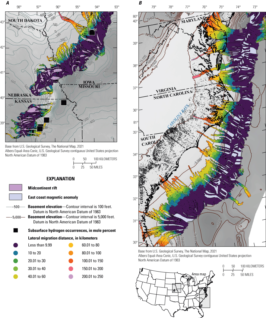
Maps showing the lateral migration from source to hydrogen occurrences. A, Migration flow pathways from a potential hydrogen source in the midcontinent rift (pink polygon in background; modified from Elling and others [2022]) show that fluid flow is directed towards known hydrogen occurrences (black squares). B, Migration flow pathways from a hypothesized source along the east coast magnetic anomaly (blue polygon in background; modified from Biari and others [2017]) show fluid flow is directed inboard towards to the onshore east coast of the United States. The distribution of Carolina bays is shown in thin black outlines (data from Lundine and Trembanis [2021]), which compares favorably with the distribution of onshore-directed flowlines. Lateral migration distance is indicated by the color scale. Contours and grey shaded background map indicate basement elevation in feet (fig. 6).
Although hydrogen occurrences have been discovered in wells targeting other natural gases or fluids (for example, water, helium, and hydrocarbons), other detections have been made with soil gas surveys. Recently, high concentrations of hydrogen in soil gas have been observed in shallow, ellipsoidal surface depressions known colloquially as “fairy circles” or Carolina bays (Zgonnik and others, 2015). These features have been theorized to be formed by processes as varied as impact craters; thermokarst lakes; or wind, wave, or groundwater processes; however, their depth and aspect ratio preclude compatibility with impact craters and thermokarst lake processes (Lundine and Trembanis, 2021). Although these features are not always associated with hydrogen degassing, a correlation between these features and elevated surface hydrogen observations has been widely supported, for example in Australia (Frery and others, 2021), Brazil (Moretti and others, 2021), Mali (Prinzhofer and others, 2018), Namibia (Moretti and others, 2022), Russia (Larin and others, 2015), and elsewhere in the United States (Zgonnik and others, 2015). Fluxes have been noted to vary rapidly throughout daily cycles (Moretti and others, 2021). The mechanism underlying the association has not been thoroughly established, although shallow transport models have sought to explain their periodicity (Myagkiy and others, 2020). In the United States, Carolina bays occur in some parts of Nebraska (known locally as the Nebraska “rainwater basins” or in Kansas as playa-lunette systems) and extensively along the eastern seaboard (Lundine and Trembanis, 2021).
The eastern seaboard of the United States is a passive margin created during the rifting of Pangea. Globally, many rifted margins are often associated with serpentinized mantle, and previous researchers have hypothesized that exhumed or otherwise serpentinized mantle rocks may exist offshore along the eastern seaboard of the United States at depth (Biari and others, 2017). We used the ECMA to delineate the rifted edge of continental crust and propose it as a potential spatial proxy for a source of subsurface hydrogen due to serpentinization. Lateral migration flow pathways from this potential source are shown in figure 12B and indicate flow updip from offshore to onshore. Many flow lines, and the drainage areas that encapsulate them (fig. 6), overlie the region of Carolina bays in the United States, from northern Florida to southern New Jersey (Lundine and Trembanis, 2021). North of the Baltimore Canyon Trough, a major basement depression off the coast of New Jersey (Grow and others, 1988), flow is redirected outboard, rather than inboard; this transition coincides with the disappearance of Carolina bays in the northeastern States. We hypothesize that Carolina bays, with sporadic hydrogen degassing, may represent the far inboard surface seepage of hydrogen that has migrated long-distance from deep, offshore serpentinized mantle-derived source rocks. If this is true, subsurface reservoirs may contain hydrogen that was trapped along this route near the coastline and offshore. Accordingly, relative increases in COS are shown in our prospectivity map, particularly along the coast of North Carolina, eastern Maryland, Delaware, and southern New Jersey, where the ECMA is particularly close to the shoreline (figs. 11 and 12). This hypothesis can be further tested by examining subsurface stratigraphic relations from offshore to onshore to characterize potential carrier beds with sufficient porosity and permeability to facilitate this migration.
Summary
Although much remains unknown and untested in the geologic hydrogen system, this study seeks to integrate basic concepts for hydrogen generation, migration, and storage to provide a useful and publicly available methodology for continental-scale mapping of geologic hydrogen prospectivity. The method has been applied in the conterminous United States and provides critical information to guide further detailed studies. Our methodology leverages decades of exploration tools and concept development from other subsurface resources to quantify spatial trends in prospectivity. As more is learned about the hydrogen system, this flexible and open methodology can be easily adapted to consider alternative or additional ideas and can be applied at a variety of spatial scales in other regions of the Earth and potentially other planets.
Acknowledgments
The authors greatly appreciate several U.S. Geological Survey colleagues for their assistance in various portions of this work. Ani Tikku is thanked for her geophysical expertise in the processing of magnetic and gravity data used for generation model layer SP4. Scott Kinney, Rob Miller, Chris Skinner, Molly O’Halloran, and Mel Zhang are thanked for their help in sourcing, compiling, and filtering various data layers used in this study. Reviews by Dave Houseknecht, Laura Dair, Isabelle Moretti, and Chris Boreham are gratefully acknowledged and significantly improved this manuscript. SLB (formerly Schlumberger) is acknowledged for the use of PetroMod migration modeling software in this work.
References Cited
Apps, J.A., and van der Kamp, P.C., 1993, Energy gases of abiotic origin in the Earth’s crust, in Howell, D.G., ed., The future of energy gases: U.S. Geological Survey Professional Paper 1570, p. 81–132, accessed November 28, 2024, at https://pubs.usgs.gov/publication/pp1570.
Bankey, V., Cuevas, A., Daniels, D., Finn, C.A., Hernandez, I., Hill, P., Kucks, R., Miles, W., Pilkington, M., Roberts, C., Roest, W., Rystrom, V., Shearer, S., Snyder, S., Sweeney, R.E., Velez, J., Phillips, J.D., and Ravat, D.K.A., 2002, Digital data grids for the magnetic anomaly map of North America: U.S. Geological Survey Open-File Report 2002–414, scale 1:10,000,000, 2 pamphlet, [variously paged; 48 p.], accessed November 28, 2024, at https://doi.org/10.3133/ofr02414.
Beauheim, R.L., and Roberts, R.M., 2002, Hydrology and hydraulic properties of a bedded evaporite formation: Journal of Hydrology, v. 259, no. 1–4, p. 66–88, accessed November 28, 2024, at https://doi.org/10.1016/S0022-1694(01)00586-8.
Biari, Y., Klingelhoefer, F., Sahabi, M., Funck, T., Benabdellouahed, M., Schnabel, M., Reichert, C., Gutscher, M.-A., Bronner, A., and Austin, J.A., 2017, Opening of the central Atlantic Ocean—Implications for geometric rifting and symmetric initial seafloor spreading after continental breakup: Tectonics, v. 36, no. 6, p. 1129–1150, accessed November 28, 2024, at https://doi.org/10.1002/2017TC004596.
Bjorlykke, K., 2010, Petroleum geoscience—From sedimentary environments to rock physics: Heidelberg, Springer-Verlag Berlin, 508 p., accessed November 28, 2024, at https://doi.org/10.1007/978-3-642-02332-3.
Blackwell, D.D., Richards, M.C., Frone, Z.S., Batir, J.F., Williams, M.A., Ruzo, A.A., and Dingwall, R.K, 2011, SMU Geothermal Laboratory heat flow map of the conterminous United States, 2011: Southern Methodist University, 1 sheet, accessed November 28, 2024, at https://www.smu.edu/dedman/academics/departments/earth-sciences/research/geothermallab/datamaps/geothermalmapofnorthamerica.
Blakely, R.J., 1995, Potential theory in gravity and magnetic applications: Cambridge, England, Cambridge University Press, 464 p., accessed November 28, 2024, at https://doi.org/10.1017/CBO9780511549816.
Blay-Roger, R., Bach, W., Bobadilla, L.F., R7amirez Reina, T., Odriozola, J.A., Amils, R., and Blay, V., 2024, Natural hydrogen in the energy transition—Fundamentals, promise, and enigmas: Renewable and Sustainable Energy Reviews, v. 189, art. 113888, 9 p., accessed November 28, 2024, at https://doi.org/10.1016/j.rser.2023.113888.
Boillot, G., Grimaud, S., Mauffret, A., Mougenot, D., Kornprobst, J., Mergoil-Daniel, J., and Torrent, G., 1980, Ocean-continent boundary off the Iberian margin—A serpentinite diapir west of the Galicia Bank: Earth and Planetary Science Letters, v. 48, no. 1, p. 23–34, accessed November 28, 2024, at https://doi.org/10.1016/0012-821X(80)90166-1.
Bonnemains, D., Carlut, J., Escartín, J., Mével, C., Andreani, M., and Debret, B., 2016, Magnetic signatures of serpentinization at ophiolite complexes: Geochemistry, Geophysics, Geosystems, v. 17, no. 8, p. 2969–2986, accessed November 28, 2024, at https://doi.org/10.1002/2016GC006321.
Boreham, C.J., Edwards, D.S., Czado, K., Rollet, N., Wang, L., van der Wielen, S., Champion, D., Blewett, R., Feitz, A., and Henson, P.A., 2021, Hydrogen in Australian natural gas—Occurrences, sources and resources: The APPEA Journal, v. 61, no. 1, p. 163–191, accessed November 28, 2024, at https://doi.org/10.1071/AJ20044.
Boreham, C.J., Edwards, D.S., Feitz, A.J., Murray, A.P., Mahlstedt, N., and Horsfield, B., 2023, Modelling of hydrogen gas generation from overmature organic matter in the Cooper Basin, Australia: The APPEA Journal, v. 63, no. 2, p. S351–S356, accessed November 28, 2024, at https://doi.org/10.1071/AJ22084.
Brennan, S.T., Rivera, J.L., Creitz, R.H., Varela, B., and Park, A.J., 2021, Natural gas compositional analyses dataset of gases from United States wells: U.S. Geological Survey data release, accessed November 28, 2024, at https://doi.org/10.5066/P9TR93E3.
Coveney, R.M., Jr., Goebel, E.D., Zeller, E.J., Dreschhoff, G.A.M., and Angino, E.E., 1987, Serpentinization and the origin of hydrogen gas in Kansas: AAPG Bulletin, v. 71, no. 1, p. 39–48, accessed November 28, 2024, at https://doi.org/10.1306/94886D3F-1704-11D7-8645000102C1865D.
Ege, J.R., 1985, Maps showing distribution, thickness, and depth of salt deposits of the United States: U.S. Geological Survey Open-File Report 1985–28, 12 p., 4 pls., accessed November 28, 2024, at https://doi.org/10.3133/ofr8528.
Elling, R., Stein, S., Stein, C.A., and Gefeke, K., 2022, Three major failed rifts in Central North America—Similarities and differences: GSA Today, v. 32, no. 6, p. 4–11, accessed November 28, 2024, at https://doi.org/10.1130/GSATG518A.1.
Ellis, G., and Gelman, S.E., 2024, Model predictions of global geologic hydrogen resources: Science Advances, v. 10, no. 50, 11 p., accessed November 28, 2024, at https://doi.org/10.1126/sciadv.ado0955.
Faure, S., 2010, World kimberlites CONSOREM database (ver. 3): Universite du Quebec a Montreal: Consortium de Recherche en Exploration Minerale database, accessed November 28, 2024, at https://consorem2.uqac.ca/production_scientifique/fiches_projets/world_kimberlites_and_lamproites_consorem_database_v2010.xls.
Frery, E., Langhi, L., Maison, M., and Moretti, I., 2021, Natural hydrogen seeps identified in the North Perth Basin, Western Australia: International Journal of Hydrogen Energy, v. 46, no. 61, p. 31158–31173, accessed November 28, 2024, at https://doi.org/10.1016/j.ijhydene.2021.07.023.
Frezon, S.E., and Finn, T.M., 1988, Map of sedimentary basins in the conterminous United States: U.S. Geological Survey Oil and Gas Investigation Map OM–223, 1 sheet, scale 1:5,000,000, accessed November 28, 2024, at https://doi.org/10.3133/om223.
Frezon, S.E., Finn, T.M., and Lister, J.M., 1983, Total thickness of sedimentary rocks in the conterminous United States: U.S. Geological Survey Open-File Report 1983–920, 1 pl., [scale approximately 1:4,836,600], accessed November 28, 2024, at https://doi.org/10.3133/ofr83920.
Frost, B.R., and Beard, J.S., 2007, On silica activity and serpentinization: Journal of Petrology, v. 48, no. 7, p. 1351–1368, accessed November 28, 2024, at https://doi.org/10.1093/petrology/egm021.
Fugelli, E.M.G., and Olsen, T.R., 2005, Risk assessment and play fairway analysis in frontier basins—Part 2—Examples from offshore mid-Norway: AAPG Bulletin, v. 89, no. 7, p. 883–896, accessed November 28, 2024, at https://doi.org/10.1306/02110504030.
Gaucher, E.C., 2020, New perspectives in the industrial exploration for native hydrogen: Elements, v. 16, no. 1, p. 8–9, accessed November 28, 2024, at https://doi.org/10.2138/gselements.16.1.8.
GEBCO Bathymetric Compilation Group, 2024, The GEBCO_2024 grid—A continuous terrain model of the global oceans and land: NERC EDS British Oceanographic Data Centre NOC dataset, accessed November 28, 2024, at https://doi.org/10.5285/1C44CE99-0A0D-5F4F-E063-7086ABC0EA0F.
Geymond, U., Ramanaidou, E., Lévy, D., Ouaya, A., and Moretti, I., 2022, Can weathering of banded iron formations generate natural hydrogen? Evidence from Australia, Brazil and South Africa: Minerals, v. 12, no. 2, art. 163, 28 p., accessed November 28, 2024, at https://doi.org/10.3390/min12020163.
Geymond, U., Briolet, T., Combaudon, V., Sissmann, O., Martinez, I., Duttine, M., and Moretti, I., 2023, Reassessing the role of magnetite during natural hydrogen generation: Frontiers in Earth Science, v. 11, art. 1169356, 11 p., accessed November 28, 2024, at https://doi.org/10.3389/feart.2023.1169356.
Gillard, M., Tugend, J., Müntener, O., Manatschal, G., Karner, G.D., Autin, J., Sauter, D., Figueredo, P.H., and Ulrich, M., 2019, The role of serpentinization and magmatism in the formation of decoupling interfaces at magma-poor rifted margins: Earth-Science Reviews, v. 196, art. 102882, 18 p., accessed November 28, 2024, at https://doi.org/10.1016/j.earscirev.2019.102882.
Gregory, S.P., Barnett, M.J., Field, L.P., and Milodowski, A.E., 2019, Subsurface microbial hydrogen cycling—Natural occurrence and implications for industry: Microorganisms, v. 7, no. 2, art. 53, 27 p., accessed November 28, 2024, at https://doi.org/10.3390/microorganisms7020053.
Grow, J. A., Klitgord, K.D., and Schlee, J.S., 1988, Structure and evolution of Baltimore Canyon Trough, in Sheridan, R.E., and Grow, J.A., eds., The Atlantic continental margin—U.S.: The Geological Society of America, v. 1–2, p. 269–290 accessed November 28, 2024, at https://doi.org/10.1130/DNAG-GNA-I2.269.
Guélard, J., Beaumont, V., Rouchon, V., Guyot, F., Pillot, D., Jézéquel, D., Ader, M., Newell, K.D., and Deville, E., 2017, Natural H2 in Kansas—Deep or shallow origin?: Geochemistry, Geophysics, Geosystems, v. 18, no. 5, p. 1841–1865, accessed November 28, 2024, at https://doi.org/10.1002/2016GC006544.
Guillot, S., Hattori, K.H., De Sigoyer, J., Nägler, T., and Auzende, A.-L., 2001, Evidence of hydration of the mantle wedge and its role in the exhumation of eclogites: Earth and Planetary Science Letters, v. 193, no. 1–2, p. 115–127, accessed November 28, 2024, at https://doi.org/10.1016/S0012-821X(01)00490-3.
Hanson, J., and Hanson, H., 2024, Hydrogen’s organic genesis: Unconventional Resources, v. 4, art. 100057, 8 p., accessed November 28, 2024, at https://doi.org/10.1016/j.uncres.2023.07.003.
Harper, G.D., 1986, Dismembered Archean ophiolite in the southeastern Wind River Mountains Wyoming—Remains of Archean oceanic crust, in deWit, M.J., and Ashwal, L.D., eds., Proceedings of a Workshop on Tectonic Evolution of Greenstone Belts, Houston, Tex., January 16–18, 1986: Houston, Tex., Lunar Planetary Institute Technical Report 86–10, p. 108, accessed November 28, 2024, at https://ui.adsabs.harvard.edu/abs/1986tegb.work..108H.
Hearon, J.S., Gelman, S.E., Ellis, G.S., Kinney, S.A., Miller, R.F., Tikku, A.A., Skinner, C.C., O'Halloran, M.M., and Zhang, M., 2025, Data release for prospectivity mapping for geologic hydrogen: U.S. Geological Survey data release, https://doi.org/10.5066/P13WCG5U.
Hirschmann, M.M., 2006, Water, melting, and the deep Earth H2O cycle: Annual Review of Earth and Planetary Sciences, v. 34, p. 629–653, accessed November 28, 2024, at https://doi.org/10.1146/annurev.earth.34.031405.125211.
Horsfield, B., Mahlstedt, N., Weniger, P., Misch, D., Vranjes-Wessely, S., Han, S., and Wang, C., 2022, Molecular hydrogen from organic sources in the deep Songliao Basin, P.R. China: International Journal of Hydrogen Energy, v. 47, no. 38, p. 16750–16774, accessed November 28, 2024, at https://doi.org/10.1016/j.ijhydene.2022.02.208.
Horton, J.D., San Juan, C.A., and Stoeser, D.B., 2017, The State Geologic Map Compilation (SGMC) geodatabase of the conterminous United States (ver. 1.1, August 2017): U.S. Geological Survey Data Series 1052, 46 p., accessed November 28, 2024, at https://doi.org/10.3133/ds1052.
Hubbert, M.K., 1953, Entrapment of petroleum under hydrodynamic conditions: AAPG Bulletin, v. 37, no. 8, p. 1954–2026, accessed November 28, 2024, at https://pubs.geoscienceworld.org/aapg/aapgbull/article-abstract/37/8/1954/33940/Entrapment-of-Petroleum-Under-Hydrodynamic.
Ingebritsen, S.E., and Manning, C.E., 2010, Permeability of the continental crust—Dynamic variations inferred from seismicity and metamorphism: Geofluids, v. 10, p. 193–205, accessed November 28, 2024, at https://doi.org/10.1111/j.1468-8123.2010.00278.x.
Ito, G., Frazer, N., Lautze, N., Thomas, D., Hinz, N., Waller, D., Whittier, R., and Wallin, E., 2017, Play fairway analysis of geothermal resources across the State of Hawaii—2. Resource probability mapping: Geothermics, v. 70, p. 393–405, accessed November 28, 2024, at https://doi.org/10.1016/j.geothermics.2016.11.004.
Jacops, E., Aertsens, M., Maes, N., Bruggeman, C., Swennen, R., Krooss, B., Amann-Hildenbrand, A., and Littke, R., 2017, The dependency of diffusion coefficients and geometric factor on the size of the diffusing molecule—Observations for different clay-based materials: Geofluids, v. 2017, art. 8652560, 16 p., accessed November 28, 2024, at https://doi.org/10.1155/2017/8652560.
Juliani, C., and Ellefmo, S.L., 2019, Multi-scale quantitative risk analysis of seabed minerals—Principles and application to seafloor massive sulfide prospects: Natural Resources Research, v. 28, p. 909–930, accessed November 28, 2024, at https://doi.org/10.1007/s11053-018-9427-y.
Krevor, S.C., Graves, C.R., Van Gosen, B.S., and McCafferty, A.E., 2009, Mapping the mineral resource base for mineral carbon-dioxide sequestration in the conterminous United States: U.S. Geological Survey Digital Data Series 414, accessed November 28, 2024, at https://pubs.usgs.gov/ds/414/.
Krivoruchko, K., and Gribov, A., 2019, Evaluation of empirical Bayesian kriging: Spatial Statistics, v. 32, art. 100368, 27 p., accessed November 28, 2024, at https://doi.org/10.1016/j.spasta.2019.100368.
Kucks, R.P., 1999, Isostatic residual gravity anomaly data grid for the conterminous US [sic]: U.S. Geological Survey dataset, accessed November 28, 2024, at https://mrdata.usgs.gov/geophysics/gravity.html. [Extracted from U.S. Geological Survey Digital Data Series DDS–9 available at https://pubs.usgs.gov/publication/ds9.]
Lamur, A., Kendrick, J.E., Eggertsson, G.H., Wall, R.J., Ashworth, J.D., and Lavallée, Y., 2017, The permeability of fractured rocks in pressurised volcanic and geothermal systems: Scientific Reports, v. 7, art. 6173, 9 p., accessed November 28, 2024, at https://doi.org/10.1038/s41598-017-05460-4.
Larin, N., Zgonnik, V., Rodina, S., Deville, E., Prinzhofer, A., and Larin, V.N., 2015, Natural molecular hydrogen seepage associated with surficial, rounded depressions on the European craton in Russia: Natural Resources Research, v. 24, p. 369–383, accessed November 28, 2024, at https://doi.org/10.1007/s11053-014-9257-5.
Lindsay, M.R., Colman, D.R., Amenabar, M.J., Fristad, K.E., Fecteau, K.M., Debes, R.V., II, Spear, J.R., Shock, E.L., Hoehler, T.M., and Boyd, E.S., 2019, Probing the geological source and biological fate of hydrogen in Yellowstone hot springs: Environmental Microbiology, v. 21, no. 10, p. 3816–3830, accessed November 28, 2024, at https://doi.org/10.1111/1462-2920.14730.
Liu, Z., Perez-Gussinye, M., García-Pintado, J., Leila Mezri, L., and Bach, W., 2023, Mantle serpentinization and associated hydrogen flux at North Atlantic magma-poor rifted margins: Geology, v. 51, no. 3, p. 284–289, accessed November 28, 2024, at https://doi.org/10.1130/G50722.1.
Loewen, M.W., Graham, D.W., Bindeman, I.N., Lupton, J.E., and Garcia, M.O., 2019, Hydrogen isotopes in high 3He/4He submarine basalts—Primordial vs. recycled water and the veil of mantle enrichment: Earth and Planetary Science Letters, v. 508, p. 62–73, accessed November 28, 2024, at https://doi.org/10.1016/j.epsl.2018.12.012.
Lottaroli, F., Craig, J., and Cozzi, A., 2018, Evaluating a vintage play fairway exercise using subsequent exploration results—Did it work?: Petroleum Geoscience, v. 24, p. 159–171, accessed November 28, 2024, at https://doi.org/10.1144/petgeo2016-150.
Lundine, M.A., and Trembanis, A.C., 2021, Using convolutional neural networks for detection and morphometric analysis of Carolina Bays from publicly available digital elevation models: Remote Sensing, v. 13, no. 18, art. 3770, 27 p., accessed November 28, 2024, at https://doi.org/10.3390/rs13183770.
Mahlstedt, N., Horsfield, B., Weniger, P., Misch, D., Shi, X., Noah, M., and Boreham, C., 2022, Molecular hydrogen from organic sources in geological systems: Journal of Natural Gas Science and Engineering, v. 105, art. 104704, 24 p., accessed November 28, 2024, at https://doi.org/10.1016/j.jngse.2022.104704.
Maiga, O., Deville, E., Laval, J., Prinzhofer, A., and Diallo, A.B., 2023, Characterization of the spontaneously recharging natural hydrogen reservoirs of Bourakebougou in Mali: Scientific Reports, v. 13, art. 11876, 13 p., accessed November 28, 2024, at https://doi.org/10.1038/s41598-023-38977-y.
Maiga, O., Deville, E., Laval, J., Prinzhofer, A., and Diallo, A.B., 2024, Trapping processes of large volumes of natural hydrogen in the subsurface—The emblematic case of the Bourakebougou H2 field in Mali: International Journal of Hydrogen Energy, v. 50, part B, p. 640–647, accessed November 28, 2024, at https://doi.org/10.1016/j.ijhydene.2023.10.131.
Malvić, T., Pimenta Dinis, M.A., Velić, J., Sremac, J., Ivšinović, J., Bošnjak, M., Barudžija, U., Veinović, Z., and Pedrosa e Sousa, H.F., 2020, Geological risk calculation through probability of success (PoS), applied to radioactive waste disposal in deep wells—A conceptual study in the pre-Neogene basement in the northern Croatia: Processes, v. 8, no. 7, art. 755, 24 p., accessed November 28, 2024, at https://doi.org/10.3390/pr8070755.
Manatschal, G., 2004, New models for evolution of magma-poor rifted margins based on a review of data and concepts from West Iberia and the Alps: International Journal of Earth Sciences, v. 93, p. 432–66, accessed November 28, 2024, at https://doi.org/10.1007/s00531-004-0394-7.
Manzer, G.K., Jr., and Heimlich, R.A., 1974, Petrology and geochemistry of mafic and ultramafic rocks from the northern Bighorn Mountains, Wyoming: Geological Society of America Bulletin, v. 85, no. 5, p. 703–708, accessed November 28, 2024, at https://pubs.geoscienceworld.org/gsa/gsabulletin/article-abstract/85/5/703/201604/Petrology-and-Geochemistry-of-Mafic-and-Ultramafic?redirectedFrom=fu lltext.
Marshak, S., Domrois, S., Abert, C., and Larson, T., 2016, DEM of the great unconformity, USA cratonic platform: Urbana-Champaign, Ill., University of Illinois at Urbana-Champaign dataset, accessed November 28, 2024, at https://doi.org/10.13012/B2IDB-7546972_V1.
McBride, J.H., and Nelson, K.D., 1988, Integration of COCORP deep reflection and magnetic anomaly analysis in the southeastern United States—Implications for origin of the Brunswick and east coast magnetic anomalies: Geological Society of America Bulletin, v. 100, no. 3, p. 436–445, accessed November 28, 2024, at https://pubs.geoscienceworld.org/gsa/gsabulletin/article-abstract/100/3/436/182136/Integration-of-COCORP-deep-reflection-and-magnetic?redirectedFrom=f ulltext.
McCafferty, A.E., San Juan, C.A., Lawley, C.J.M., Graham, G.E., Gadd, M.G., Huston, D.L., Kelley, K.D., Paradis, S., Peter, J.M., and Czarnota, K., 2023, National-scale geophysical, geologic, and mineral resource data and grids for the United States, Canada, and Australia—Data in support of the tri-national Critical Minerals Mapping Initiative: U.S. Geological Survey data release, accessed November 28, 2024, at https://doi.org/10.5066/P970GDD5.
McCollom, T.M., and Bach, W., 2009, Thermodynamic constraints on hydrogen generation during serpentinization of ultramafic rocks: Geochimica et Cosmochimica Acta, v. 73, no. 3, p. 856–875, accessed November 28, 2024, at https://doi.org/10.1016/j.gca.2008.10.032.
McKenzie, D., 1978, Some remarks on the development of sedimentary basins: Earth and Planetary Science Letters, v. 40, no. 1, p. 25–32, accessed November 28, 2024, at https://doi.org/10.1016/0012-821X(78)90071-7.
Milkov, A.V., 2022, Molecular hydrogen in surface and subsurface natural gases—Abundance, origins and ideas for deliberate exploration: Earth-Science Reviews, v. 230, art. 104063, 27 p., accessed November 28, 2024, at https://doi.org/10.1016/j.earscirev.2022.104063.
Moretti, I., Geymond, U., Pasquet, G., Aimar, L., and Rabaute, A., 2022, Natural hydrogen emanations in Namibia—Field acquisition and vegetation indexes from multispectral satellite image analysis: International Journal of Hydrogen Energy, v. 47, no. 84, p. 35588–35607, accessed November 28, 2024, at https://doi.org/10.1016/j.ijhydene.2022.08.135.
Moretti, I., Prinzhofer, A., Françolin, J., Pacheco, C., Rosanne, M., Rupin, F., and Mertens, J., 2021, Long-term monitoring of natural hydrogen superficial emissions in a Brazilian cratonic environment—Sporadic large pulses versus daily periodic emissions: International Journal of Hydrogen Energy, v. 46, no. 5, p. 3615–3628, accessed November 28, 2024, at https://doi.org/10.1016/j.ijhydene.2020.11.026.
Myagkiy, A., Moretti, I., and Brunet, F., 2020, Space and time distribution of subsurface H2 concentration in so-called “fairy circles”—Insight from a conceptual 2-D transport model: BSGF Earth Sciences Bulletin, v. 191, art. 13, 13 p., accessed November 28, 2024, at https://doi.org/10.1051/bsgf/2020010.
Oakey, G.N., and Saltus, R.W., 2016, Geophysical analysis of the Alpha–Mendeleev ridge complex—Characterization of the High Arctic Large Igneous Province: Tectonophysics, v. 691, part A, p. 65–84, accessed November 28, 2024, at https://doi.org/10.1016/j.tecto.2016.08.005.
Ohira, I., Ohtani, E., Sakai, T., Miyahara, M., Hirao, N., Ohishi, Y., and Nishijima, M., 2014, Stability of a hydrous δ-phase, AlOOH–MgSiO2(OH)2, and a mechanism for water transport into the base of lower mantle: Earth and Planetary Science Letters, v. 401, p. 12–17, accessed November 28, 2024, at https://doi.org/10.1016/j.epsl.2014.05.059.
Olson, P.L., and Sharp, Z.D., 2022, Primordial helium‐3 exchange between Earth’s core and mantle: Geochemistry, Geophysics, Geosystems, v. 23, no. 3, art. e2021GC009985, 18 p., accessed November 28, 2024, at https://doi.org/10.1029/2021GC009985.
Osselin, F., Soulaine, C., Fauguerolles, C., Gaucher, E.C., Scaillet, B., and Pichavant, M., 2022, Orange hydrogen is the new green: Nature Geoscience, v. 15, no. 10, p. 765–769, accessed November 28, 2024, at https://doi.org/10.1038/s41561-022-01043-9.
Otis, R.M., and Schneidermann, N., 1997, A process for evaluating exploration prospects: AAPG Bulletin, v. 81, no. 7, p. 1087–1109, accessed November 28, 2024, at https://doi.org/10.1306/522B49F1-1727-11D7-8645000102C1865D.
Potts, M.J., 1972, Origin of a Precambrian ultramafic intrusion in southeastern Wyoming, U.S.A.: Contributions to Mineralogy and Petrology, v. 36, no. 4, p. 249–264, accessed November 28, 2024, at https://doi.org/10.1007/BF00444335.
Prinzhofer, A., and Cacas-Stentz, M.-C., 2023, Natural hydrogen and blend gas—A dynamic model of accumulation: International Journal of Hydrogen Energy, v. 48, no. 57, p. 21610–21623, accessed November 28, 2024, at https://doi.org/10.1016/j.ijhydene.2023.03.060.
Prinzhofer, A., Tahara Cissé, C.S., and Diallo, A.B., 2018, Discovery of a large accumulation of natural hydrogen in Bourakebougou (Mali): International Journal of Hydrogen Energy, v. 43, no. 42, p. 19315–19326, accessed November 28, 2024, at https://doi.org/10.1016/j.ijhydene.2018.08.193.
Sherwood Lollar, B., Onstott, T.C., Lacrampe-Couloume, G., and Ballentine, C.J., 2014, The contribution of the Precambrian continental lithosphere to global H2 production: Nature, v. 516, p. 379–382, accessed November 28, 2024, at https://doi.org/10.1038/nature14017.
Skinner, C.C., Miller, R.F., Kinney, S.A., Gianoutsos, N.J., Gunther, G.L., and Shorten, C.M., 2022, Aggregated oil and natural gas drilling and production history of the United States (ver. 1.1, April 2023): U.S. Geological Survey data release, accessed November 28, 2024, at https://doi.org/10.5066/P9UIR5HE.
SLB, 2020, PetroMod (ver. 2020.1, April 2020): SLB software release, accessed November 28, 2024, at https://www.software.slb.com/software-news/software-top-news/petromod/petromod-2020-1. [Formerly Schlumberger.]
Smith, N.J.P., Shepherd, T.J., Styles, M.T., and Williams, G.M., 2005, Hydrogen exploration—A review of global hydrogen accumulations and implications for prospective areas in NW Europe: London, Geological Society, Petroleum Geology Conference Series, v. 6, p. 349–358, accessed November 28, 2024, at https://doi.org/10.1144/0060349.
Smith-Schmitz, S.E., and Appold, M.S., 2022, Reactive transport modeling of the role of fluorine-rich groundwater in the formation of fluorite ore deposits in the Illinois-Kentucky District, USA: Hydrogeology Journal, v. 30, p. 1199–1218, accessed November 28, 2024, at https://doi.org/10.1007/s10040-022-02479-4.
Spear, J.R., Walker, J.J., McCollom, T.M., and Pace, N.R., 2005, Hydrogen and bioenergetics in the Yellowstone geothermal ecosystem: Proceedings of the National Academy of Sciences, v. 102, no. 7, p. 2555–2560, accessed November 28, 2024, at https://doi.org/10.1073/pnas.0409574102.
Speziale, L., and Geneletti, D., 2014, Applying an ecosystem services approach to support land-use planning—A case study in Koboko district, Uganda: Ecological Processes, v. 3, art. 10, 13 p., accessed November 28, 2024, at https://doi.org/10.1186/2192-1709-3-10.
Tissot, B.P., and Welte, D.H., 1984, Petroleum formation and occurrence (2d ed.): Heidelberg, Springer-Verlag Berlin, 702 p., accessed November 28, 2024, at https://doi.org/10.1007/978-3-642-87813-8.
Tóth, J., 1962, A theory of groundwater motion in small drainage basins in central Alberta, Canada: Journal of Geophysical Research, v. 67, no. 11, p. 4375–4388, accessed November 28, 2024, at https://doi.org/10.1029/JZ067i011p04375.
U.S. Energy Information Administration 2020a, Uranium—Identified resource areas: U.S. Energy Information Administration dataset, accessed November 28, 2024, at https://atlas.eia.gov/datasets/eia::uranium-identified-resource-areas/about.
U.S. Energy Information Administration, 2020b, Uranium—NURE favorable areas: U.S. Energy Information Administration dataset, accessed November 28, 2024, at https://atlas.eia.gov/datasets/eia::uranium-nure-favorable-areas/about.
U.S. Geological Survey [USGS], 2019, Energy geochemistry database: U.S. Geological Survey provisional database, accessed November 28, 2024, at https://certmapper.cr.usgs.gov/data/apps/geochem-db/.
Wang, L., Cheng, J., Jin, Z., Sun, Q., Zou, R., Meng, Q., Liu, K., Su, Y., and Zhang, Q., 2023, High-pressure hydrogen adsorption in clay minerals—Insights on natural hydrogen exploration: Fuel, v. 344, art. 127919, 12 p., accessed November 28, 2024, https://doi.org/10.1016/j.fuel.2023.127919.
White, D.A., 1993, Geologic risking guide for prospects and plays: AAPG Bulletin, v. 77, no. 12, p. 2048–2061, accessed November 28, 2024, at https://doi.org/10.1306/BDFF8FCE-1718-11D7-8645000102C1865D.
Whitmeyer, S.J., and Karlstrom, K.E., 2007, Tectonic model for the Proterozoic growth of North America: Geosphere, v. 3, no. 4, p. 220–259, accessed November 28, 2024, at https://doi.org/10.1130/GES00055.1.
Williams, Q., and Hemley, R.J., 2001, Hydrogen in the deep Earth: Annual Review of Earth and Planetary Sciences, v. 29, p. 365–418, accessed November 28, 2024, at https://doi.org/10.1146/annurev.earth.29.1.365.
Wu, Y., Louden, K.E., Funck, T., Jackson, H.R., and Dehler, S.A., 2006, Crustal structure of the central Nova Scotia margin off Eastern Canada: Geophysical Journal International, v. 166, no. 2, p. 878–906, accessed November 28, 2024, at https://doi.org/10.1111/j.1365-246X.2006.02991.x.
Zgonnik, V., 2020, The occurrence and geoscience of natural hydrogen—A comprehensive review: Earth-Science Reviews, v. 203, art. 103140, 51 p., accessed November 28, 2024, at https://doi.org/10.1016/j.earscirev.2020.103140.
Zgonnik, V., Beaumont, V., Deville, E., Larin, N., Pillot, D., and Farrell, K.M., 2015, Evidence for natural molecular hydrogen seepage associated with Carolina Bays (surficial, ovoid depressions on the Atlantic coastal plain, province of the USA): Progress in Earth and Planetary Science, v. 2, art. 31, 15 p., accessed November 28, 2024, at https://doi.org/10.1186/s40645-015-0062-5.
Appendix 1. Supplementary Figures
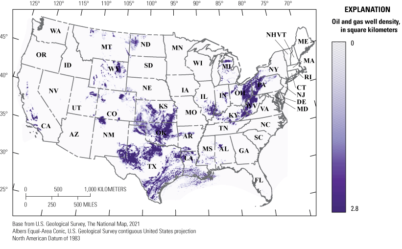
Density map showing the distribution of previously drilled wells that produced either oil or hydrocarbon gas in the conterminous United States (data from Skinner and others [2022]). Dry holes are not included in this compilation since some of these may include previously unrecognized hydrogen gas.
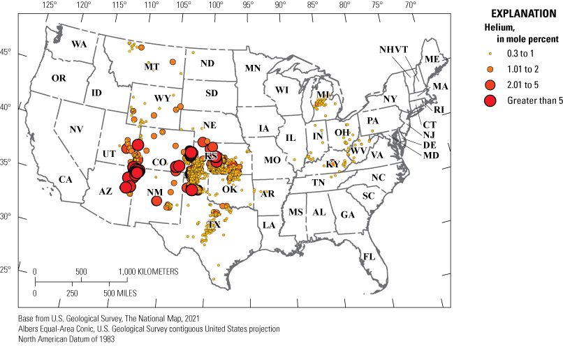
Map showing reported concentrations of helium from oil and gas wells with greater than 0.3 mole percent (mol%) in gas samples throughout the conterminous United States (data from U.S. Geological Survey [2019] and Brennan and others [2021]). Symbol size qualitatively correlates with concentration.
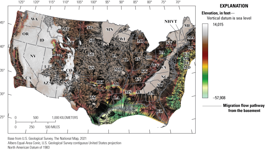
High resolution map showing hydrogen migration flow lines throughout the conterminous United States in regions with sedimentary cover.
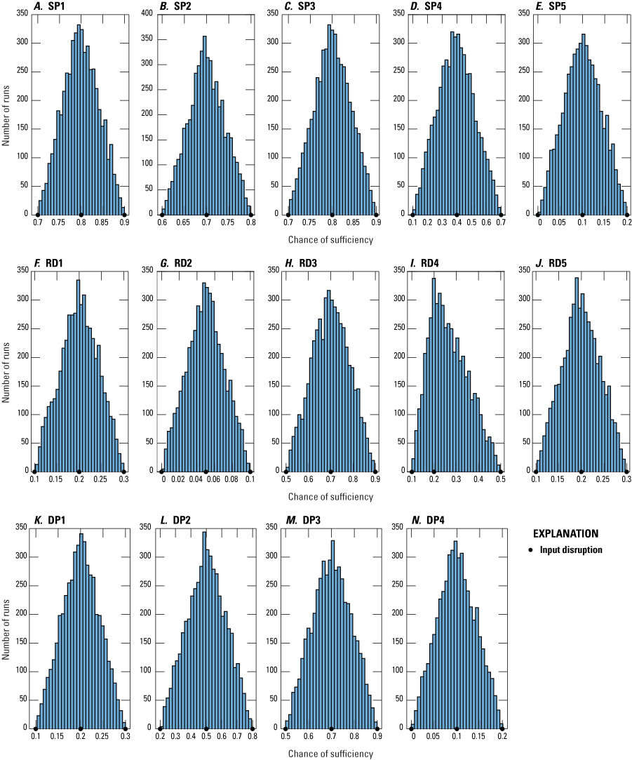
Graphs showing input distributions for Monte Carlo model for source subcomponent layers. A total of 5,000 stochastic simulations were calculated to generate the final prospectivity map. Input distributions are defined by low, mid, and high chance of sufficiency (COS) values given in table 1 and are indicated with black circles. A–E, Serpentinization (SP) layers SP1–SP5, F–J, radiolysis (RD) layers RD1–RD5, and K–N, deep sources (DP) input layers DP1–DP4 are defined by triangular distributions.
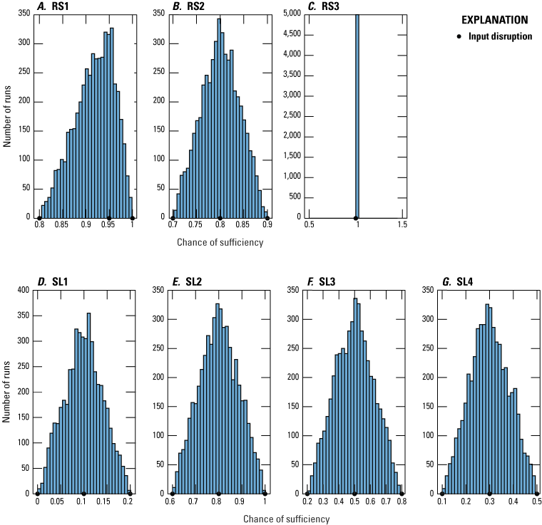
Graphs showing the input distributions for Monte Carlo model for reservoir and seal component layers. A total of 5,000 stochastic simulations were calculated to generate the final prospectivity map. Input distributions are defined by low, mid, and high chance of sufficiency (COS) values defined in table 1 and are indicated with black circles. A–C, Reservoir (RS) and D–G, seal (SL) input layers RS1–RS3 and SL1–SL4 are defined by triangular distributions.
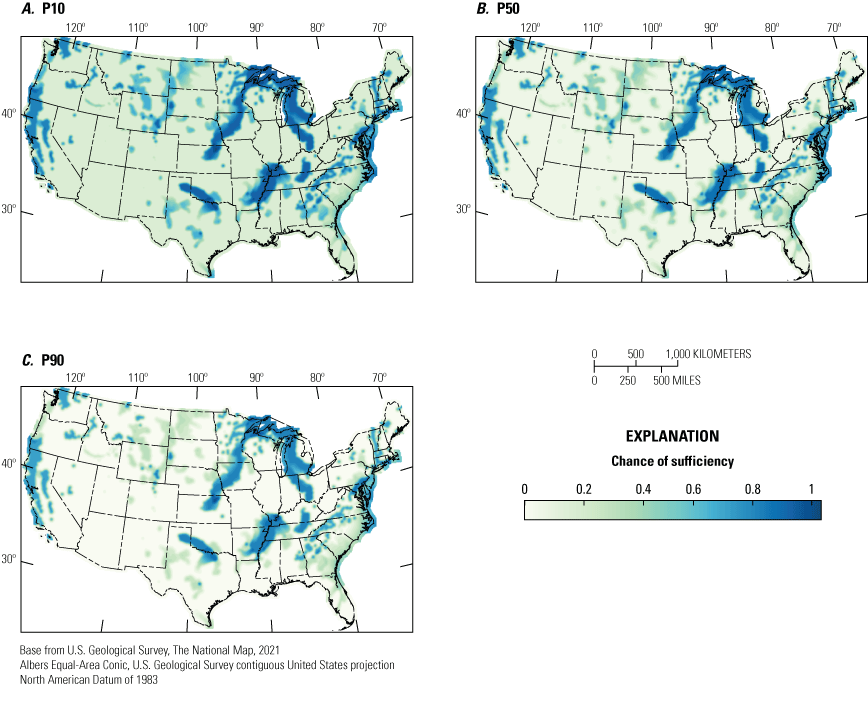
Maps showing the Monte Carlo results for serpentinization source COS. Stochastic results are plotted for 5,000 simulations showing the A, 10 percent of runs exceed this chance of sufficiency (COS) value; B, the P50, that is 50 percent of runs exceed this COS value; and C, P90, that is 90 percent of runs exceed this COS value.
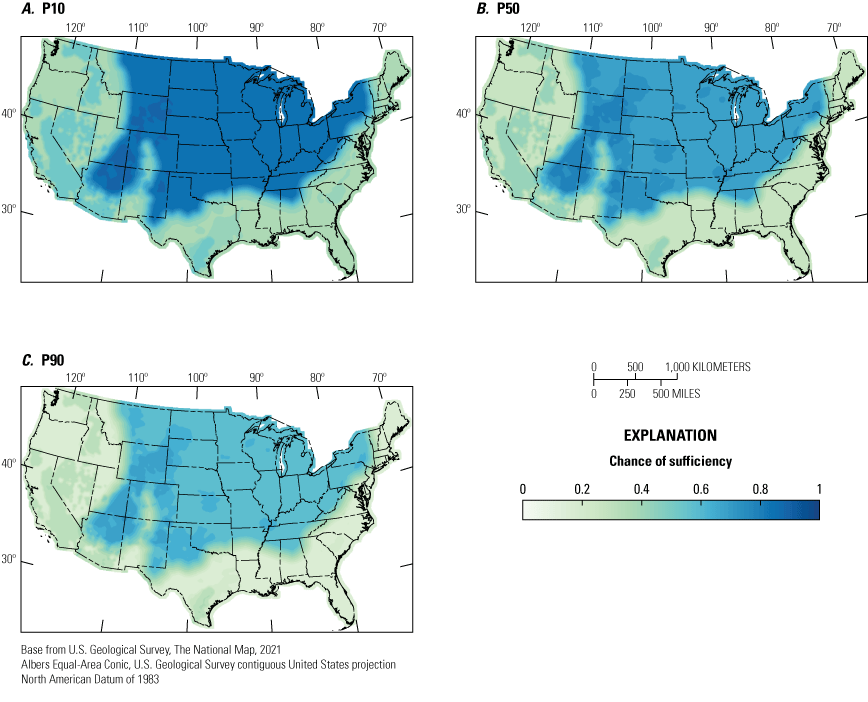
Maps showing the Monte Carlo results for radiolysis source. Stochastic results are plotted for 5,000 simulations showing the A, P10, that is 10 percent of runs exceed this chance of sufficiency (COS) value; B, P50, that is 50 percent of runs exceed this COS value; and C, P90, that is 90 percent of runs exceed this COS value.

Maps showing the Monte Carlo results for deep source. Stochastic results are plotted for 5,000 simulations showing the A, P10, that is 10 percent of runs exceed this chance of sufficiency (COS) value; B, P50, that is 50 percent of runs exceed this COS value; and C, P90, that is 90 percent of runs exceed this COS value.
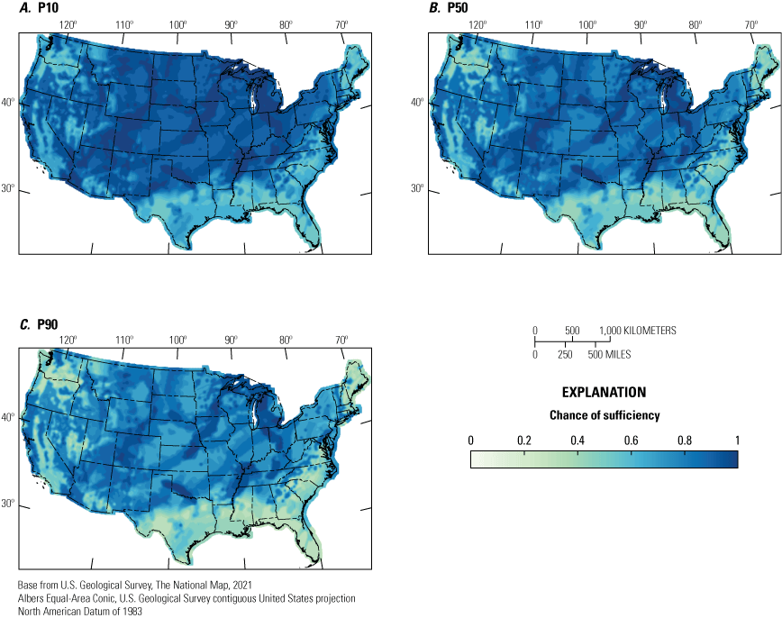
Maps showing the Monte Carlo results for the composite source. Stochastic results are plotted for 5,000 simulations showing the A, P10, that is 10 percent of runs exceed this chance of sufficiency (COS) value; B, P50, that is 50 percent of runs exceed this COS value; and C, P90, that is 90 percent of runs exceed this COS value.

Maps showing the Monte Carlo results for the composite reservoir. Stochastic results are plotted for 5,000 simulations showing the A, P10, that is 10 percent of runs exceed this chance of sufficiency (COS) value; B, P50, that is 50 percent of runs exceed this COS value; and C, P90, that is 90 percent of runs exceed this COS value.

Maps showing the Monte Carlo results for the composite seal. Stochastic results are plotted for 5,000 simulations showing the A, P10, that is 10 percent of runs exceed this COS value; B, P50, that is 50 percent of runs exceed this COS value; and C, P90, that is 90 percent of runs exceed this COS value.
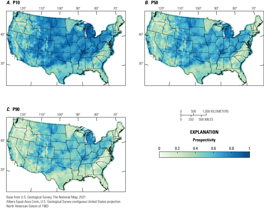
Maps showing the Monte Carlo results for final prospectivity. Stochastic results are plotted for 5,000 simulations showing the A, 10 percent exceedance probability (P10), B, 50 percent exceedance probability (P50) and C, 90 percent exceedance probability (P90) values. Exceedance probabilities describe the statistical likelihood that a particular prospectivity value will be exceeded. A P10 map displays the prospectivity value at each mapped location that 10% of simulation runs exceed.
Appendix 2. Matlab Script to Calculate Prospectivity
% Sarah Gelman
% H2 Favorability Version 1
% May 21, 2024

format long g;
set(groot,'DefaultFigureColor','white')
set(groot,'DefaultAxesBox','on')
set(groot,'DefaultAxesXGrid','on')
set(groot,'DefaultAxesYGrid','on')

clear all; close all; clc;

write_output = 0;

grid_interval = 5;

%% Set the COS weights.

range_sp1 = 0.8;
range_sp2 = 0.7;
range_sp3 = 0.8;
range_sp4 = 0.4;
range_sp5 = 0.1;

range_rd1 = 0.2;
range_rd2 = 0.05;
range_rd3 = 0.7;
range_rd4 = 0.2;
range_rd5 = 0.2;

range_dp1 = 0.2;
range_dp2 = 0.5;
range_dp3 = 0.7;
range_dp4 = 0.1;

range_rs1 = 0.95;
range_rs2 = 0.8;
range_rs3 = 1.0;

range_sl1 = 0.1;
range_sl2 = 0.8;
range_sl3 = 0.5;
range_sl4 = 0.3;


%% Load grids.
% CHANGE FILE NAMES ACCORDINGLY.

[SP1_orig,R_sp1] = readgeoraster('src_sp1_emca.asc');
SP1_orig = single(SP1_orig);
[SP2_orig,R_sp2] = readgeoraster('src_sp2_surfaceumafic.asc');
SP2_orig = single(SP2_orig);
[SP3_orig,R_sp3] = readgeoraster('src_sp3_failedrifts.asc');
SP3_orig = single(SP3_orig);
[SP4_orig,R_sp4] = readgeoraster('src_sp4_geophysics.asc');
SP4_orig = single(SP4_orig);

[RD1_orig,R_rd1] = readgeoraster('src_rd1_uraniumdep.asc');
RD1_orig = single(RD1_orig);
[RD2_orig,R_rd2] = readgeoraster('src_rd2_uraniumfav.asc');
RD2_orig = single(RD2_orig);
[RD3_orig,R_rd3] = readgeoraster('src_rd3_craton.asc');
RD3_orig = single(RD3_orig);
[RD4_orig,R_rd4] = readgeoraster('src_rd4_accreted.asc');
RD4_orig = single(RD4_orig);
[RD5_orig,R_rd5] = readgeoraster('src_rd5_kgranites.asc');
RD5_orig = single(RD5_orig);

[DP1_orig,R_dp1] = readgeoraster('src_dp1_faults.asc');
DP1_orig = single(DP1_orig);
[DP2_orig,R_dp2] = readgeoraster('src_dp2_sutures.asc');
DP2_orig = single(DP2_orig);
[DP3_orig,R_dp3] = readgeoraster('src_dp3_highheat.asc');
DP3_orig = single(DP3_orig);

[RS1_orig,R_rs1] = readgeoraster('res_rs1_sedrocks.asc');
RS1_orig = single(RS1_orig);
[RS2_orig,R_rs2] = readgeoraster('res_rs2_nonsedrocks.asc');
RS2_orig = single(RS2_orig);
[RS3_orig,R_rs3] = readgeoraster('res_rs3_sedbasin.asc');
RS3_orig = single(RS3_orig);

[SL1_orig,R_sl1] = readgeoraster('seal_sl1_salt.asc');
SL1_orig = single(SL1_orig);
[SL2_orig,R_sl2] = readgeoraster('res_rs1_sedrocks.asc');
SL2_orig = single(SL2_orig);
[SL3_orig,R_sl3] = readgeoraster('res_rs2_nonsedrocks.asc');
SL3_orig = single(SL3_orig);
[SL4_orig,R_sl4] = readgeoraster('res_rs3_sedbasin.asc');
SL4_orig = single(SL4_orig);


%% Downsample all of the grids'cell size, for monte carlo memory-sake.


x_orig = (R_sp2.XWorldLimits(1)+(R_sp2.CellExtentInWorldX/2):R_sp2.CellExtentInWorldX:R_sp2.XWorldLimits(2)-(R_sp2.CellExtentInWorldX/2))';
y_orig = R_sp2.YWorldLimits(1)+(R_sp2.CellExtentInWorldY/2):R_sp2.CellExtentInWorldY:R_sp2.YWorldLimits(2)-(R_sp2.CellExtentInWorldY/2);

x_new = (R_sp2.XWorldLimits(1)+(R_sp2.CellExtentInWorldX/2):R_sp2.CellExtentInWorldX*grid_interval:R_sp2.XWorldLimits(2)-(R_sp2.CellExtentInWorldX/2))';
y_new = R_sp2.YWorldLimits(1)+(R_sp2.CellExtentInWorldY/2):R_sp2.CellExtentInWorldY*grid_interval:R_sp2.YWorldLimits(2)-(R_sp2.CellExtentInWorldY/2);

F_SP1 = griddedInterpolant({y_orig,x_orig},SP1_orig); SP1 = F_SP1({y_new,x_new});
F_SP2 = griddedInterpolant({y_orig,x_orig},SP2_orig); SP2 = F_SP2({y_new,x_new});
F_SP3 = griddedInterpolant({y_orig,x_orig},SP3_orig); SP3 = F_SP3({y_new,x_new});
F_SP4 = griddedInterpolant({y_orig,x_orig},SP4_orig); SP4 = F_SP4({y_new,x_new});

F_RD1 = griddedInterpolant({y_orig,x_orig},RD1_orig); RD1 = F_RD1({y_new,x_new});
F_RD2 = griddedInterpolant({y_orig,x_orig},RD2_orig); RD2 = F_RD2({y_new,x_new});
F_RD3 = griddedInterpolant({y_orig,x_orig},RD3_orig); RD3 = F_RD3({y_new,x_new});
F_RD4 = griddedInterpolant({y_orig,x_orig},RD4_orig); RD4 = F_RD4({y_new,x_new});
F_RD5 = griddedInterpolant({y_orig,x_orig},RD5_orig); RD5 = F_RD5({y_new,x_new});

F_DP1 = griddedInterpolant({y_orig,x_orig},DP1_orig); DP1 = F_DP1({y_new,x_new});
F_DP2 = griddedInterpolant({y_orig,x_orig},DP2_orig); DP2 = F_DP2({y_new,x_new});
F_DP3 = griddedInterpolant({y_orig,x_orig},DP3_orig); DP3 = F_DP3({y_new,x_new});

F_RS1 = griddedInterpolant({y_orig,x_orig},RS1_orig); RS1 = F_RS1({y_new,x_new});
F_RS2 = griddedInterpolant({y_orig,x_orig},RS2_orig); RS2 = F_RS2({y_new,x_new});
F_RS3 = griddedInterpolant({y_orig,x_orig},RS3_orig); RS3 = F_RS3({y_new,x_new});

F_SL1 = griddedInterpolant({y_orig,x_orig},SL1_orig); SL1 = F_SL1({y_new,x_new});
F_SL2 = griddedInterpolant({y_orig,x_orig},SL2_orig); SL2 = F_SL2({y_new,x_new});
F_SL3 = griddedInterpolant({y_orig,x_orig},SL3_orig); SL3 = F_SL3({y_new,x_new});
F_SL4 = griddedInterpolant({y_orig,x_orig},SL4_orig); SL4 = F_SL4({y_new,x_new});

%% Smooth all of the input grids.

% Replace all the nan values with actual NaNs.
SP1(SP1==-9999) = NaN;
SP2(SP2==-9999) = NaN;
SP3(SP3==-9999) = NaN;
SP4(SP4==-9999) = NaN;

RD1(RD1==-9999) = NaN;
RD2(RD2==-9999) = NaN;
RD3(RD3==-9999) = NaN;
RD4(RD4==-9999) = NaN;
RD5(RD5==-9999) = NaN;

DP1(DP1==-9999) = NaN;
DP2(DP2==-9999) = NaN;
DP3(DP3==-9999) = NaN;

RS1(RS1==-9999) = NaN;
RS2(RS2==-9999) = NaN;
RS3(RS3==-9999) = NaN;

SL1(SL1==-9999) = NaN;
SL2(SL2==-9999) = NaN;
SL3(SL3==-9999) = NaN;
SL4(SL4==-9999) = NaN;


%% Determine the AOI.

nlong = length(SP1(1,:));
nlat = length(SP1(:,1));

AOI_subs = find(SL1>=0);
[AOI_lat,AOI_long] = ind2sub([nlat nlong],AOI_subs);

ncells = length(AOI_subs);

%% Calculate the deterministic prospectivity map. (Testing).

% Calculate the Source COS.
% Serpentinization COS.
cos_sp = 1-((1-(range_sp1*SP1(AOI_subs))).*(1-(range_sp2*SP2(AOI_subs))).*...
    (1-(range_sp3*SP3(AOI_subs))).*(1-(range_sp4*SP4(AOI_subs))).*(1-(range_sp5)));

% Radiolysis COS.
cos_rd = 1-((1-(range_rd1*RD1(AOI_subs))).*(1-(range_rd2*RD2(AOI_subs))).*...
    (1-(range_rd3*RD3(AOI_subs))).*(1-(range_rd4*RD4(AOI_subs))).*...
    (1-(range_rd5*RD5(AOI_subs))));

% Deep Source COS.
cos_dp = 1-((1-(range_dp1*DP1(AOI_subs))).*(1-(range_dp2*DP2(AOI_subs))).*...
    (1-(range_dp3*DP3(AOI_subs))).*(1-(range_dp4)));

% Calculate the total source COS.
cos_sc = 1-((1-cos_sp).*(1-cos_rd).*(1-cos_dp));

% Calculate the Reservoir COS.
cos_rs = 1-((1-(range_rs1*RS1(AOI_subs))).*(1-(range_rs2*RS2(AOI_subs))).*...
    (1-(range_rs3*RS3(AOI_subs))));

% Calculate the Seal COS.
cos_sl = 1-((1-(range_sl1*SL1(AOI_subs))).*(1-(range_sl2*SL2(AOI_subs))).*...
    (1-(range_sl3*SL3(AOI_subs))).*(1-(range_sl4*SL4(AOI_subs))));

% Calculate the total prospectivity.
P = cos_sc.*cos_rs.*cos_sl;


%% Write out outputs.

cos_sp_gd = NaN*ones(nlat,nlong);
cos_rd_gd = NaN*ones(nlat,nlong);
cos_dp_gd = NaN*ones(nlat,nlong);
cos_rs_gd = NaN*ones(nlat,nlong);
cos_sl_gd = NaN*ones(nlat,nlong);
cos_sc_gd = NaN*ones(nlat,nlong);
p_gd = NaN*ones(nlat,nlong);

% Convert everything back to a grid format from linear indexing.

for i = 1:length(AOI_subs)
    row = AOI_lat(i); col = AOI_long(i);
    cos_sp_gd(row,col) = cos_sp(i);
    cos_rd_gd(row,col) = cos_rd(i);
    cos_dp_gd(row,col) = cos_dp(i);
    cos_sc_gd(row,col) = cos_sc(i);
    cos_rs_gd(row,col) = cos_rs(i);
    cos_sl_gd(row,col) = cos_sl(i);
    p_gd(row,col) = P(i);
end

%% Smooth the final grids at the end of the calculation!
smooth_window = 10;

cos_sp_gd = smoothdata2(cos_sp_gd,"gaussian",smooth_window); cos_sp_gd = smoothdata2(cos_sp_gd,"gaussian",smooth_window/2);
cos_rd_gd = smoothdata2(cos_rd_gd,"gaussian",smooth_window); cos_rd_gd = smoothdata2(cos_rd_gd,"gaussian",smooth_window/2);
cos_dp_gd = smoothdata2(cos_dp_gd,"gaussian",smooth_window); cos_dp_gd = smoothdata2(cos_dp_gd,"gaussian",smooth_window/2);
cos_sc_gd = smoothdata2(cos_sc_gd,"gaussian",smooth_window); cos_sc_gd = smoothdata2(cos_sc_gd,"gaussian",smooth_window/2);
cos_rs_gd = smoothdata2(cos_rs_gd,"gaussian",smooth_window); cos_rs_gd = smoothdata2(cos_rs_gd,"gaussian",smooth_window/2);
cos_sl_gd = smoothdata2(cos_sl_gd,"gaussian",smooth_window); cos_sl_gd = smoothdata2(cos_sl_gd,"gaussian",smooth_window/2);
p_gd = smoothdata2(p_gd,"gaussian",smooth_window); p_gd = smoothdata2(p_gd,"gaussian",smooth_window/2);

%% Plot results.

stoplight_colormap = [165,0,38;...
    215,48,39;...
    244,109,67;...
    253,174,97;...
    254,224,139;...
    217,239,139;...
    166,217,106;...
    102,189,99;...
    26,152,80;...
    0,104,55]./255;

% Interpolate the colorbar.
cb1 = interp1([1:10]',stoplight_colormap(:,1),[1:0.25:10]');
cb2 = interp1([1:10]',stoplight_colormap(:,2),[1:0.25:10]');
cb3 = interp1([1:10]',stoplight_colormap(:,3),[1:0.25:10]');
stoplight_colormap_hr = [cb1,cb2,cb3];


figure('Position',[500 100 1600 800]); h = imagesc(cos_sp_gd,[0 1]); set(h,'AlphaData',~isnan(cos_sp_gd)); colormap(stoplight_colormap_hr); title('Combined COS Serpentinization Deterministic'); axis equal; colorbar;

figure('Position',[500 100 1600 800]); h = imagesc(cos_rd_gd,[0 1]); set(h,'AlphaData',~isnan(cos_rd_gd)); colormap(stoplight_colormap_hr); title('Combined COS Radiolysis Deterministic'); axis equal; colorbar;

figure('Position',[500 100 1600 800]); h = imagesc(cos_dp_gd,[0 1]); set(h,'AlphaData',~isnan(cos_dp_gd)); colormap(stoplight_colormap_hr); title('Combined COS Deep Sources Deterministic'); axis equal; colorbar;

figure('Position',[500 100 1600 800]); h = imagesc(cos_sc_gd,[0 1]); set(h,'AlphaData',~isnan(cos_sc_gd)); colormap(stoplight_colormap_hr); title('Combined Source COS Deterministic'); axis equal; colorbar;

figure('Position',[500 100 1600 800]); h = imagesc(cos_rs_gd,[0 1]); set(h,'AlphaData',~isnan(cos_rs_gd)); colormap(stoplight_colormap_hr); title('Reservoir COS Deterministic'); axis equal; colorbar;

figure('Position',[500 100 1600 800]); h = imagesc(cos_sl_gd,[0 1]); set(h,'AlphaData',~isnan(cos_sl_gd)); colormap(stoplight_colormap_hr); title('Seal COS Deterministic'); axis equal; colorbar;

figure('Position',[500 100 1600 800]); h = imagesc(p_gd,[0 1]); set(h,'AlphaData',~isnan(p_gd)); colormap(stoplight_colormap_hr); title('Total Combined Prospectivity Deterministic'); axis equal; colorbar;
Conversion Factors
Datums
Horizontal coordinate information is referenced to the North American Datum of 1983 (NAD 83).
Elevation, as used in this report, refers to distance above the mean sea level.
Abbreviations
COS
chance of sufficiency
DP
deep sources of hydrogen subcomponent
ECMA
east coast magnetic anomaly
GIS
geographic information systems
mol%
mole percent
mol% H2
mole percent hydrogen
P
prospectivity
RD
radiolysis subcomponent
RS
reservoir component
RTP
reduced-to-pole
SC
source component
SL
seal component
SP
serpentinization subcomponent
USGS
U.S. Geological Survey
Publishing support provided by the Science Publishing Network, Denver and Reston Publishing Service Centers
For more information concerning the research in this report, contact the Center Director, USGS Central Energy Resources Science Center
Box 25046, Mail Stop 939
Denver, CO 80225
(303) 236-1647
Or visit the Central Energy Resources Science Center website at https://www.usgs.gov/centers/central-energy-resources-science-center
Disclaimers
Any use of trade, firm, or product names is for descriptive purposes only and does not imply endorsement by the U.S. Government.
Although this information product, for the most part, is in the public domain, it also may contain copyrighted materials as noted in the text. Permission to reproduce copyrighted items must be secured from the copyright owner.
Suggested Citation
Gelman, S.E., Hearon, J.S., and Ellis, G.S., 2025, Prospectivity mapping for geologic hydrogen (ver. 1.2, January 22, 2025): U.S. Geological Survey Professional Paper 1900, 43 p., https://doi.org/10.3133/pp1900.
ISSN: 2330-7102 (online)
Study Area
| Publication type | Report |
|---|---|
| Publication Subtype | USGS Numbered Series |
| Title | Prospectivity mapping for geologic hydrogen |
| Series title | Professional Paper |
| Series number | 1900 |
| DOI | 10.3133/pp1900 |
| Edition | Version 1: January 16, 2025; Version 1.1: January 17, 2025; Version 1.2: January 22, 2025 |
| Publication Date | January 16, 2025 |
| Year Published | 2025 |
| Language | English |
| Publisher | U.S. Geological Survey |
| Publisher location | Reston VA |
| Contributing office(s) | Central Energy Resources Science Center |
| Description | Report: iv, 43 p.; Data Release |
| Country | United States |
| Other Geospatial | conterminous United States |
| Online Only (Y/N) | Y |