

Numerical Modeling of Groundwater Flow in the Crystalline-Rock Aquifer in the Vicinity of the Savage Municipal Water-Supply Well Superfund Site, Milford, New Hampshire
Links
- Document: Report (12.2 MB pdf) , HTML , XML
- Data Release: USGS data release - MODFLOW -2005, MODPATH, and MOC3D used for groundwater flow simulation, pathlines analysis, and solute transport in the crystalline-rock aquifer in the vicinity of the Savage Municipal Water-Supply Well Superfund site, Milford, New Hampshire
- Download citation as: RIS | Dublin Core
Acknowledgments
This study was completed as part of characterization and remediation efforts at the Savage Municipal Water-Supply Well Superfund site and is a collaborative effort between Federal, State, and local government agencies and private companies and individuals. The author wishes to thank Gerardo Millan-Ramos, current site remedial project manager, and Richard Hull, former site manager, both from the U.S. Environmental Protection Agency, and Robin Mongeon, project manager from the New Hampshire Department of Environmental Services, for their leadership in managing remediation efforts and their support.
Abstract
In 2010, tetrachloroethylene (PCE), a chlorinated volatile organic compound, was detected in groundwater from deep (more than 300 feet below land surface) fractures in monitoring wells tapping a crystalline-rock aquifer. The aquifer underlies the Milford-Souhegan glacial-drift aquifer, a high water-producing aquifer, and the Savage Municipal Water-Supply Well Superfund site in Milford, New Hampshire. Between 30 and 40 residential water-supply wells are near (0.25 mile north of) the PCE-contaminated monitoring wells. Some of the residential water-supply wells are likely installed in similar rock types and formations as those of the monitoring wells installed as part of the Superfund site. As of 2020, periodic sampling by the U.S. Environmental Protection Agency and New Hampshire Department of Environmental Services (cooperative partners for this study) since 1996 had not detected PCE in groundwater from the residential water-supply wells. Nevertheless, understanding the vulnerability of the residential water wells to capture PCE contaminated groundwater was of concern.
A numerical groundwater flow model was developed by the U.S. Geological Survey to assess groundwater flow and advective transport of PCE-contaminated groundwater in the crystalline-rock aquifer of the Milford area. The model (called the area-wide model) encompasses a 26.5-square mile area to allow for more accurate computation of water fluxes near the PCE-contaminated monitoring wells and the residential water wells. Simulations with the area-wide model show that, with the 2016 configuration of residential wells, capture of PCE by the residential water wells appears unlikely for hydrologic conditions typical of 2010 based on steady-state, advective transport modeling. However, simulations also show that adding residential water wells to the north of the PCE-contaminated monitoring wells could affect the transport of PCE. Groundwater withdrawals at other adjacent wells in the overlying Milford-Souhegan glacial-drift aquifer affect advective transport in the crystalline-rock aquifer. Therefore, the potential for future changes in withdrawals in the area, as well as changes in hydrologic conditions, including groundwater recharge and streamflow amounts, should be considered in the remedial assessment process. The development of the area-wide model and linkages established by this study with previously developed Milford-Souhegan glacial-drift aquifer transport models will help facilitate the development of remedial strategies for this Superfund site.
Introduction
High concentrations (more than 3,000 parts per billion [ppb]) of tetrachloroethylene [PCE]), a chlorinated volatile organic compound, were detected in groundwater in 2010 from deep (more than 300 feet [ft] below land surface [bls]) fractures in monitoring wells tapping a crystalline-rock aquifer beneath operable unit 1 (OU1) of the Savage Municipal Water-Supply Well Superfund site in Milford, New Hampshire (Weston Solutions, Inc., 2010). Operable units define remedial areas of contaminant concern. The areal extent of PCE concentrations in the bedrock that are more than 1,000 ppb, as reported in Weston Solutions, Inc. (2010), is generally confined to areas south of the Souhegan River (fig. 1). PCE contamination previously was detected in the overlying glacial sand and gravel deposits and basal till, hereafter referred to as the Milford-Souhegan glacial drift (MSGD) aquifer, as early as 1983 (Harte, 2004, 2006). The primary original source of contamination for OU1 has been identified as a former O.K. Tool Co., Inc., manufacturing facility (HMM Associates, Inc., 1991; Weston Solutions, Inc., 2010).
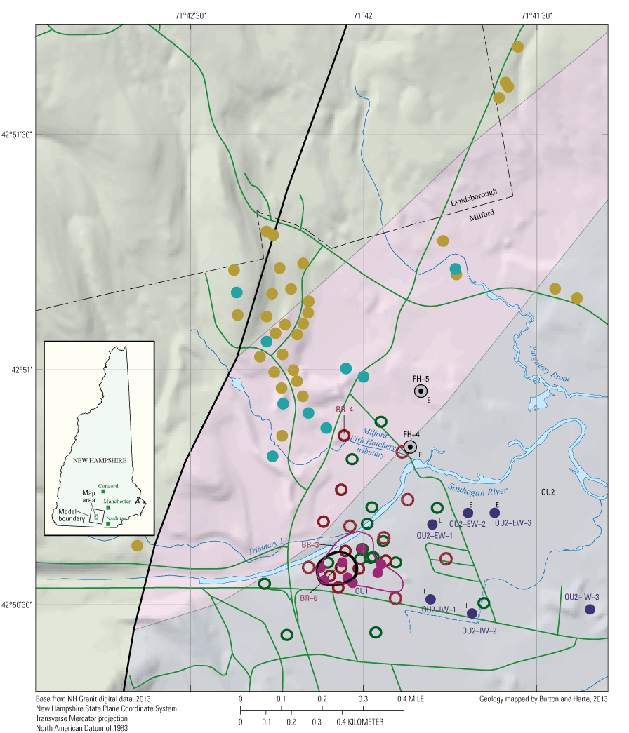
Map showing the locations of selected monitoring wells and bedrock residential water-supply wells near the Savage Municipal Water-Supply Well Superfund site, Milford, New Hampshire. OU1 is the primary source area of tetrachloroethylene (PCE), and OU2 is the extended plume area of PCE. PCE was detected in well BR–3; no PCE was detected in well BR–4. ft, feet; msl, mean sea level; ppb, parts per billion; >, greater than; <, less than.
Thirty to 40 residential water-supply wells are in close proximity (approximately 0.25 mile north) from the PCE-contaminated monitoring wells and the area delineated with bedrock PCE concentrations more than 1,000 ppb (fig. 1). Residential water-supply wells are likely installed in similar rocks (granite and gneiss) as the monitoring wells as interpreted by overlaying well locations with formations mapped on the New Hampshire State geologic map (fig. 1; Bennett and others, 2006). More residential water wells were constructed in the early 1990s. After the discovery of PCE contamination in groundwater from deep fractures in 2010, an investigation began in that same year by the U.S. Environmental Protection Agency (EPA) and the New Hampshire Department of Environmental Services (NHDES) to assess the potential for PCE transport from known contaminant locations to the residential water wells. The U.S. Geological Survey (USGS) and the EPA entered into an interagency agreement in 2011 and a cooperative agreement with the NHDES in 2012 to help assess PCE transport in the crystalline-rock aquifer from known PCE concentration areas.
Periodic sampling by the EPA and the NHDES from 1996 to 2020 had not detected PCE in groundwater from the residential water-supply wells. However, part of assessing the potential for PCE transport involves understanding the movement of groundwater in the crystalline-rock aquifer. One of the tools for understanding movement of groundwater, particularly in complex, highly heterogeneous crystalline-rock aquifers, is numerical modeling of groundwater flow (Harte and Winter, 1995; Tiedeman and others, 1997; Mack, 2009). This report describes the development of a numerical groundwater-flow model and summarizes findings from simulations of flow in the crystalline-rock aquifer of the Milford area. The model is called the area-wide model (fig. 2) because it encompasses a relatively large area (26.5 square miles). By having the model cover a large area, distal water fluxes that contribute flow to the residential water-supply wells and the area shown in figure 1 can be more accurately computed. According to Reilly and Harbaugh (2004), “The extent of the model is expanded outward from the area of concern both vertically and horizontally so that the physical extent coincides with physical features of the groundwater system that can be represented as boundaries.” Furthermore, fluxes computed by the area-wide model can be used as input to existing models for the area of interest to improve simulations and better account for flow into and out of the bedrock. For this report, the area of interest refers to the areal extent shown in figure 1, whereas the model area refers to the larger area covered by the area-wide model.
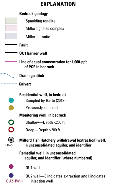
Map showing geologic rock types of the crystalline-rock aquifer and residential water-supply well yields as a ratio of yield per foot of well opening for the area-wide model in the vicinity of the Savage Municipal Water-Supply Well Superfund site, Milford, New Hampshire. MSGD, Milford-Souhegan glacial-drift.
Hydrogeology
The glaciated northeastern United States in areas underlain by crystalline rock is characterized by generally shallow depths to water (less than 30 ft bls) because the bulk permeability of the bedrock is low and recharge is relatively high (Harte and Winter, 1995). Bedrock exposures are few. A mantle of glacial till or recent alluvium overlying the bedrock in the uplands and stratified-drift deposits commonly overly the bedrock in the valleys. Flow is primarily through fractures that were created by a combination of cooling, uplift, and structural deformity. Nonfractured rock blocks have low (less than 5 percent) primary porosity (Zhou and others, 2007). Flow is often proportionally greater at shallower depths (less than 300 ft bls) than flow at deeper depths in the bedrock; although highly transmissive fractures at deep depths have been intercepted by wells. Nevertheless, the transmissivity of the bedrock is typically several orders of magnitude less than the overlying unconsolidated sediments. Transmissivities of crystalline-rock aquifers are typically less than 1,000 feet squared per day (Tiedeman and others, 1997), whereas transmissivities between 2,500 and 50,000 feet squared per day have been measured for the stratified-drift aquifers of the northeast (Randall, 2001).
Surface water and groundwater interactions are an important part of the groundwater system in the glaciated northeastern United States. Surface water recharges the groundwater where upland streams cross permeable deposits in the valleys. Surface water also can recharge the groundwater where there are large changes in the bulk permeability of an aquifer in valleys (Harte and Kiah, 2009). Groundwater discharges to surface water in uplands and valleys, but particularly in valleys.
In rural areas of the northeast, residential water-supply wells and monitoring wells open to the crystalline-rock aquifer intersect multiple fractures over the open interval of the well (open borehole). Groundwater, therefore, mixes in the borehole from the contribution of groundwater flow from multiple fractures (Harte, 2013).
In the model area, most of the uplands above altitudes of more than 330 ft mean sea level (msl) surrounding OU1 are served by residential wells set in the crystalline-rock aquifer (fig. 2). Most residential wells outside the MSGD aquifer are in the uplands. Yields of residential water wells range from 0.13 to 150 gallons per minute (gal/min) with an average of approximately 13 gal/min (New Hampshire Department of Environmental Services, written commun., 2011). The median well depth for residential water wells is 400 ft bls (an average of 421 ft bls). Most monitoring wells in OU1 are drilled to similar depths.
The crystalline-rock aquifer that underlies the model area consists of tonalite, granite, and gneiss (figs. 1 and 2; Bennett and others, 2006). Some metapelite strings are present in the uplands. Burton and Harte (2013) mapped the metapelite strings in the uplands coincident with a schist unit. Tonalite is mapped to the west and lies within the higher terrain. Tonalite is separated from the granite and gneiss to the east in the Milford-Souhegan River Valley (Bennett and others, 2006; Burton and Harte, 2013) by the Campbell Hill Fault (figs. 1 and 2). The fault appears to be primarily a normal fault that also may have a strike slip component (Burton and Harte, 2013). The position of the Campbell Hill fault is shown in Burton and Harte (2013) approximately 900 ft to the east of that shown in Bennett and others (2006) and in figure 1.
Fractures are predominantly northeast striking and steeply inclined (more than 45 degrees [°]; Weston Solutions, Inc., 2012; Burton and Harte, 2013) and dip to the northwest. The placement of the area of interest on the western limb of the Massabesic anticlinorium is likely a major factor in the number of foliation features and fractures that dip to the northwest (Burton and Harte, 2013). Water-yielding fractures generally occur every 30 to 80 ft in a borehole; fractures, whether water bearing, low permeability, or unconnected, occur every 5 to 10 ft. Although some wells drilled 500 to 600 ft into bedrock have negligible water-bearing yield.
Lineaments are linear features seen on the surface of the Earth with remotely sensed imagery. Lineaments are potentially related to structural features and high-water yielding zones within the bedrock (Mabee and Hardcastle, 1997). Lineaments were mapped in the area coincident with the area-wide model by Clark and others (1997). For the nearby Pinardville quadrangle (fig. 2), Moore and others (2002) documented statistical differences in well yield (higher) with wells along lineaments that coincide with the regional fracture directions observed at outcrops (primarily trending north-northeast).
The hydraulic conductivity of the rock is inferred from residential water well yields reported from driller logs because of widespread availability of driller logs in the State. Moore and others (2002) documented relatively high well yields associated with tonalite rocks in the USGS 7.5-minute Pinardville quadrangle directly to the northeast of the model area. They also determined tonalite rocks statewide had relatively high yields. Tonalite rocks extend from the Pinardville to the Milford quadrangle (fig. 2). The model area comprises the northern one-half of the Milford quadrangle. Wells in the gneiss rocks tended to have low yields.
Well yields normalized by the open borehole length of the well are shown in figure 2. Normalizing yields per open length provide insight into the bulk, nondirectional, hydraulic conductivity of the rock. Although not shown, lineaments do not appear to play a factor in well yield and by association the hydraulic conductivity of the rock except for the lineaments mapped coincident with the Campbell Hill Fault. The residential water wells north of OU1 appear to have a higher bulk hydraulic conductivity than other wells. These wells are proximal to the Campbell Hill fault and the contact between upland tonalite and valley granite and gneiss.
Harte (2013) sampled several residential wells near OU1 for chemical and isotopic analysis (fig. 1). These residential well data were used to infer the degree of mixing in boreholes and the origin of groundwater recharging the wells. Residential water well water was determined to have characteristics of being derived from short and long flow path lengths (Harte, 2013). Long flow paths were hypothesized as potentially being able to transport PCE given the distances of residential water wells from contamination areas. However, several of the wells with water characterized as originating from long flow paths were adjacent to the hillside where it was more likely that flow paths came from the western hillsides rather than from PCE-contaminated areas to the south and east.
The surficial aquifer of the Milford quadrangle, which covers the entire model area, was mapped by Koteff (1970). The Milford-Souhegan River Valley is directly underlain by alluvium and glacially derived sand and gravel that in turn overlie thin, discontinuous glacial till mantling bedrock (Harte, 2010). The sand and gravel and till units are discontinuous, but one of the two is generally present because bedrock exposure is limited. The highly permeable sand and gravel ranges from 50 to 130 ft in thickness and constitutes most of the MSGD aquifer (Harte and Mack, 1992; Harte, 2010). The horizontal hydraulic conductivity of the most permeable units was simulated at 450 feet per day (ft/d) in the MSGD aquifer model by Harte and others (1999). North and south of the Milford-Souhegan River Valley, the landscape is dominated by abundant glacial deposits, including till and glacial outwash, with relatively sparse bedrock outcrops (Koteff, 1970). The till has a hydraulic conductivity typically less than 10 ft/d (Harte, 2010).
Remedial Systems
The unconsolidated sediments of the MSGD aquifer have been undergoing cleanup by a pump and treat method to help contain and capture the dissolved PCE plume that is associated with the Savage Municipal Water-Supply Well Superfund site. Pump and treat cleanup started in 1999 in OU1 and in 2004 in OU2 (Gradient Corp., 2011). In addition to the OU1 pump and treat system, a low permeability, slurry barrier wall encircles areas of potential PCE source areas in the form of dense nonaqueous phase liquids or sorbed contaminated sediments. The barrier wall was installed in late 1998 and sits atop the bedrock or is keyed several feet into the till. The location of the barrier wall, OU1 pumping and injection points where treated effluent is injected back into the aquifer, and selected OU2 pumping and injection wells are shown in figure 1.
Previous and Current Numerical Modeling Investigations
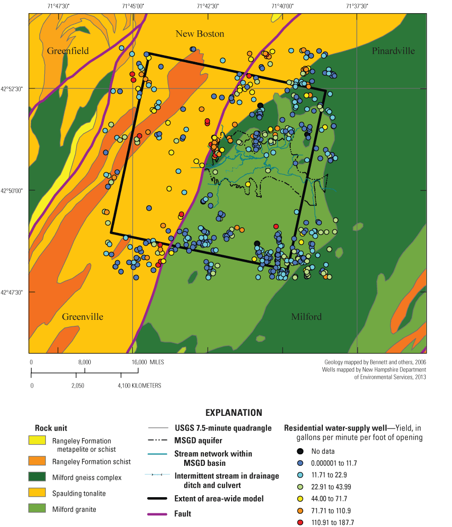
Several numerical models of flow and transport have been constructed for the unconsolidated sediments of the MSGD aquifer (table 1). However, previous models did not explicitly simulate the underlying crystalline-rock aquifer. Previous models constructed for the Milford-Souhegan River Valley included Harte and Mack (1992) and for the western one-half of the valley that focused on the Savage Municipal Water-Supply Well Superfund site previous models included Harte and others (1999). The areal extent of previous models and the area-wide model of flow are shown in figure 3. All models use some form of the USGS three-dimensional finite-difference groundwater-flow model (MODFLOW; U.S. Geological Survey, 2014).
Table 1.
Groundwater flow models for the Milford area, Savage Municipal Water-Supply Well Superfund site, Milford, New Hampshire.[Model extents shown in figure 3. MODFLOW–88 is from McDonald and Harbaugh (1988); MODFLOW–96 is from Harbaugh and McDonald (1996); MOC3D is from Konikow and others (1996); MODFLOW–GWT is from Heberton and others (2000) and U.S. Geological Survey (2011); MT3D is from Zheng (1990); MT3D99 is from Zheng and Wang (1999) and Zheng and others (2001); MODFLOW–2005 is from Harbaugh (2005). OU, operable unit; PCE, tetrachloroethylene; MODFLOW, modular three-dimensional finite-difference groundwater flow model; MODFLOW–GWT, groundwater transport module of MODFLOW; MOC3D and MT3D99, three-dimensional method-of-characteristics groundwater flow and solute transport models; MT3D, modular three-dimensional groundwater solute transport model; NA, not applicable]
| Model report | Areal extent | Simulated hydrogeologic units | Primary objective | Model code |
|---|---|---|---|---|
| Harte and Mack (1992) | Milford-Souhegan River valley | Milford-Souhegan glacial drift aquifer | Delineation of capture zones for the Savage and Keyes wells | MODFLOW–88 |
| Harte and others (1999) | Western half of the Milford-Souhegan River valley covering the Savage Municipal Water-Supply Well Superfund site | Western half of Milford- Souhegan glacial drift aquifer | Calibration of groundwater flow model and simulation of advective transport of the OU1–OU2 PCE plume | MODFLOW–88 |
| Harte (2004) | Western half of the Milford-Souhegan River valley covering the Savage Municipal Water-Supply Well Superfund site | NA | Simulation of solute transport for the OU1–OU2 PCE plume | MODFLOW–96, MOC3D, MODFLOW–GWT |
| U.S. Environmental Protection Agency (2002) | Derivative of the Harte and others (1999) and Harte (2004) models; simulated western half of the Milford-Souhegan River valley covering the Savage Municipal Water-Supply Well Superfund site | NA | Simulation of remedial options for the PCE plume and OU2 part of the Savage site | MODFLOW–96 and MT3D |
| Gradient Corp. (2002) | Derivative of the U.S. Environmental Protection Agency (2002) model; simulated western half of the Milford-Souhegan River valley covering the Savage Municipal Water-Supply Well Superfund site | NA | Simulation of remedial options for the PCE plume and OU2 part of the Savage site | MODFLOW–96 and MT3D99 |
| Harte (2012) | Western half of the Milford-Souhegan River valley covering the Savage Municipal Water-Supply Well Superfund site | NA | Simulation of selected remedial operations for the PCE plume and OU1–OU2 part of the Savage site | MODFLOW–96, MOC3D, MODFLOW–GWT |
| Area-wide model (this report) | Northern quarter of the Milford quadrangle (U.S. Geological Survey, 1:24,000) | Bedrock units of Milford quadrangle, Milford-Souhegan glacial drift aquifer and surrounding unconsolidated sediments | Simulation of flow in the crystalline-rock aquifer for the surrounding area | MODFLOW–2005 |
Map showing the areal extent of the area-wide model and of previous models of the Milford-Souhegan glacial-drift (MSGD) aquifer and the extent of the aquifer in the vicinity of the Savage Municipal Water-Supply Well Superfund site, Milford, New Hampshire.
The areal extent of models is informed by the modeling objectives of a study. For previous models, simulations focused on the MSGD aquifer and the PCE plume contained therein; the areal and vertical extents were limited to the unconsolidated sediments in the Milford Souhegan River Valley (fig. 3; table 1). With the discovery of PCE in deep fractures in the underlying crystalline-rock aquifer, the need to understand and quantify flow and transport in the crystalline-rock aquifer became crucial in the assessment of strategies for remediation. The area-wide model simulates flow in the crystalline-rock aquifer and covers a much larger area than previous models with the goal of improving the computation of groundwater flow from distal locations to the residential water wells and the area shown in figure 1. The model is also aligned with the primary fracture strike direction as mapped by Burton and Harte (2013).
Model Construction
A finite-difference numerical groundwater flow model was constructed using the USGS MODFLOW–2005 (version 1.10) platform. All model input and output files, from simulations discussed in this report, are available in Harte and Watt (2021).
For this model (figs. 2 and 3), the aquifer layers option of MODFLOW–2005 (Harbaugh, 2005) was used to specify cell hydraulic properties. The harmonic mean method was used to specify interblock conductances between cells. Three hydrogeologic units were simulated with eight model layers: the sand and gravel unit (stratified drift and recent alluvium; layer 1), the glacial till (layer 2), and the underlying crystalline-rock aquifer (layers 3 through 8). The crystalline-rock aquifer was simulated as an equivalent porous medium in as much as the bulk flow in the rock was simulated by approximating trends in the distribution of fracture permeability and flow. The sand and gravel and the till units are discontinuously simulated, but typically one of the two is present because bedrock exposure is limited. The crystalline-rock aquifer is simulated as contiguous.
All model layers are simulated with the confined option of MODFLOW–2005 (specified thickness approximation; Sheets and others, 2015) to avoid simulating dewatering of cells in the upland areas (more than 330 ft land surface). Specifying model layers as confined introduces some inaccuracy but allows for a quicker model solution. Inaccuracies result from the inability of cells to be partially saturated. Partial saturation occurs under unconfined conditions. Therefore, the bulk transmissivity of cells in the area-wide model is not saturation dependent. The error is inconsequential for cells in the lowermost layers but introduces various levels of inaccuracy for the uppermost active cells. Inaccuracy is roughly proportional to the ratio of the unsaturated to saturated thickness multiplied by the total thickness of the cell; further detail on potential errors can be found in Sheets and others (2015). Some thin till cells appeared in the simulations as numerically dewatered.
Simulated Units and Hydraulic Properties
Simulated units include the glacial stratified-drift deposits (termed sand and gravel in this report), glacial till, and the underlying bedrock. The areal extent of the sand and gravel unit was restricted to land surface altitudes less than 330 ft to match general patterns observed by Koteff (1970) in the Milford-Souhegan River Valley. The areal extent of the till was primarily continuous. The areal extent of the bedrock was simulated as continuous throughout the active model area. Some sand and gravel units have been mapped by Toppin (1987) in adjacent river valleys above altitudes of 330 ft; however, these units are not simulated in the area-wide model because they are assumed to have negligible effect on flow in the area of interest (fig. 1).
Each hydrogeologic unit (sand and gravel, till, and bedrock) was assigned unique hydraulic properties. Simulated hydraulic properties included hydraulic conductivity (horizontal and vertical hydraulic conductivity), storage coefficient for transient simulations, and porosity for simulations of advective transport.
The hydrogeologic units (sand and gravel and till) initially were specified as horizontally homogeneous. However, during the calibration process and to better replicate previously published models of the MSGD, spatial heterogeneity was introduced into the sand and gravel unit. The horizontal hydraulic conductivity (kh)of the sand and gravel unit typically was set at least one order of magnitude greater than that of the till, following regional and local hydraulic information on stratified drift deposits and tills (Toppin, 1987; Melvin and others, 1992; Harte, 2010). The kh of the till was initially set at 3 ft/d, similar to kh rates for the till in previously published MSGD aquifer models. The kh of the bedrock was initially set at one order of magnitude less than the till (0.3 ft/d) and initially specified as horizontally homogeneous. Similar to the sand and gravel unit, spatial heterogeneity was incorporated into the bedrock during the calibration process for selected simulations. This spatial heterogeneity was introduced into model layers of the bedrock by incorporating kh values calculated from hydraulic testing with straddle packers of bedrock fractures detected with borehole geophysical logging (Weston Solutions, Inc., 2012). The kh of the bedrock was assigned to appropriate model layers based on vertical positioning. Between bedrock wells, the assigned kh was interpolated by using a point inverse distance algorithm (Winston, 2009). Bedrock kh also was adjusted based on rock type (Bennett and others, 2006) and the Campbell Hill Fault location (Burton and Harte, 2013). Bedrock kh was not adjusted based on mapped lineaments (Clark and others, 1997) because of the lack of observable trends between lineament locations and well yield for the Milford area, excluding lineament features associated with the Campbell Hill Fault.
The vertical hydraulic conductivity (kv) of the sand and gravel was set at 0.10 to 0.25 of the kh, respectively, to account for layered units found in the MSGD aquifer (Harte, 2010). The kv for the till was set the same as the kh of the till. The kv for the bedrock layers was initially set equal to kh. Many of the water-bearing fractures are steeply inclined (more than 45° slope), which facilitates vertical flow (Weston Solutions, Inc. 2012). During calibration, the kv of the bedrock was increased to a multiple of the kh to better simulate inclined fractures.
Simulated Conditions
A long-term average annual preremediation (before the barrier wall and remedial system were installed in OU1) period (pre-1998) was simulated under steady-state conditions (long-term mean simulation). A quasiequilibrium simulated period, which represents the time before an aquifer test (before December 6, 2010) but postremediation (after the barrier wall and remedial system were installed in OU1) period, was simulated also under steady-state conditions (early December 2010 simulation). Finally, a short-term dynamic period representing an aquifer test that was completed during December 6 and 9, 2010, when pumping of well BR–6 (fig. 1) occurred was simulated under transient conditions (short-pump test simulation). Results from the December 2010 simulations were used as the initial conditions for the short-pump test simulations.
Discretization
The model boundaries and subsequently discretization is aligned with the principal strike and dip direction of the fractured rock. Model columns are parallel to strike and rows parallel to dip direction. The horizontal grid spacing in the model ranges from 110 to 220 ft in the row direction and 73 to 220 ft in the column direction (fig. 4). The smaller cell sizes cover the area of interest (fig. 1). The total number of cells per layer is 36,966 (202 rows by 183 columns), which totals 295,728 cells (8 layers) for the model.
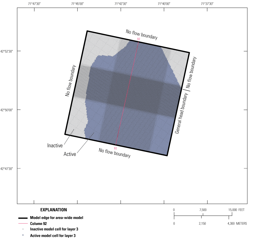
Map showing horizontal grid cells and active and inactive regions for the bedrock layers, in the area-wide model, Savage Municipal Water-Supply Superfund site, Milford, New Hampshire.
The model was constructed with eight model layers (fig. 5). The sand and gravel unit is assigned to layer 1 at altitudes less than 330 ft. The thickness of the sand and gravel unit varies from discontinuous (zero) to more than 100 ft. The till unit is assigned to layers 1 and 2 at altitudes equal to and greater than 330 ft. The thickness of the till unit typically varies from 1 to 3 ft in the valley. In some river valleys, the till is actually absent; for those areas in the model the till is specified as a thin layer (less than 1 ft) to avoid creating a discontinuity in simulated layers. Specifying a thin till layer has little effect on the vertical flow between the sand and gravel unit and the bedrock because flow is primarily controlled by the hydraulic properties of the upper bedrock. No adjustment of hydraulic properties of the till was specified for this condition besides specifying a thin layer.
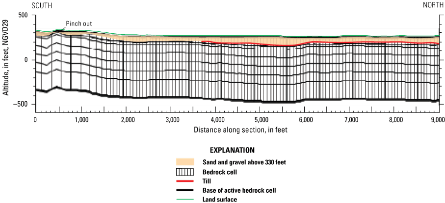
Cross section through column 92 of the area-wide model, Savage Municipal Water-Supply Superfund site, Milford, New Hampshire.
The underlying bedrock is assigned to the bottom six layers. The thickness of the uppermost bedrock layer (model layer 3) is 30 ft, which represents the maximum length of well casing penetrating the bedrock; typically, casing is 20 ft long. The well casing is impermeable, and no residential water-supply wells are simulated as open to layer 3. Bedrock layers 2 through 5 (model layers 4 through 7) are 100 ft thick. The lowermost bedrock layer (model layer 8) is 200 ft thick. The maximum simulated thickness is approximately 800 ft.
Hydrologic Boundaries
The area of the model is larger than the area of interest so that all lateral model boundaries should have a negligible effect on groundwater flow in the area of interest (fig. 1). The capture zones (zones contributing flow) of the residential water-supply wells to the north of OU1 likely extend to the west, into the uplands. The ability to delineate capture zones would be adversely affected if capture zones intersect inaccurately assigned lateral boundaries, such as a no-flow boundary where appreciable flow might occur. If affected by model lateral boundaries, capture zones might inaccurately extend farther to the south increasing the likelihood of capturing PCE-contaminated groundwater. Therefore, extending the model allows for an improved assessment of the potential capture of PCE-contaminated groundwater by the residential water-supply wells. Risk susceptibility based on potential capture of contaminated groundwater by residential water wells can further inform decision makers on the appropriateness of certain remedies in reducing risk.
The upper boundary of the model is a specified-flux condition to simulate areal recharge. The lowermost boundary is considered a no-flow boundary based on the hypothesis that open, hydraulically active fractures below this depth are less frequent than above this depth and that these deep fractures do not contribute appreciable flow to the simulated flow system. In addition, the model assumes that no appreciable deep underflow from outside the simulated area discharges or interacts with flow in the model area. The model edges are also no-flow boundaries except for the southeastern corner of the model, which is a head-dependent flux boundary for all model layers (fig. 4). Most model edges are aligned with local topographic highs where it is hypothesized that the underlying water table is high, forming a divide, and a subdued reflection of the topography because of the low bulk permeability of the bedrock (Harte and Winter, 1995). For the southeast corner edge boundary, specifying all layers as a head-dependent flux boundary promotes lateral groundwater flow and reduces upward discharge from the bedrock to the overlying unconsolidated sediments in that area. The actively simulated area along the southeastern part of the model boundary coincides with drainages that flow into the Milford-Souhegan River Valley and adjacent river valleys to the south, therefore some lateral flow is accounted for in the model.
Streams are a hydraulic boundary. Perennial streams were simulated with the River package of MODFLOW–2005 (Harbaugh, 2005). Digital stream coverages were obtained from NH Granit (2012) databases. Stream stage, streambed altitude (determined from water depth), and conductance (channel width, length, bed thickness, and hydraulic conductivity of bed material) were assigned based on previously collected data (Harte and others, 1997). In general, streams above an altitude of 330 ft were assigned narrow channels (5 ft across), shallow depth of water (less than 2 ft), and thin streambeds (1 ft thick). Conversely, streams below an altitude of 330 ft were assigned wide channels (as much as 60 ft across), greater depths of water (as much as 4 ft), and thick streambeds (3 ft thick). The hydraulic conductivity of the streambed was set at 3 ft/d in most areas based on work by Harte and others (1999).
Recharge and Groundwater Withdrawals
Areal recharge from precipitation and snowmelt was specified based on altitude. Where the land surface altitude was more than 330 ft, recharge was initially set at 0.5 foot per year (ft/yr). Where the land altitude was less than or equal to 330 ft, recharge was initially set at 2 ft/yr. Rates of recharge match published rates from Harte and Winter (1995) for upland areas and Harte and others (1999) for valleys. Recharge rates were allowed to vary during calibration for long-term mean annual and December 2010 simulations but were constrained in that the valley recharge was at least three times that of the uplands. For short-pump test simulations, recharge was applied during the first stress period (steady-state) but not applied during the subsequent transient stress periods to match the dry weather conditions immediately before and during the aquifer test.
Groundwater withdrawals varied based on the period of the simulation (table 2). For long-term mean annual simulation, groundwater withdrawals were simulated from residential water-supply wells drilled into the bedrock, withdrawals from wells at the New Hampshire Fish and Game Department’s Milford Fish Hatchery at Milford, N.H., and withdrawals from several other commercial wells. Rates of withdrawals were specified from New Hampshire water use reports (New Hampshire Department of Environmental Services, undated; Genevieve Al-Egaily, New Hampshire Department of Environmental Services, written commun., August 2, 2010), for commercial wells or estimated from typical per capita water use amounts for residential water-supply wells (Carolyn Hayek, U.S. Geological Survey, written commun., 2009). For the December 2010 simulations, additional groundwater withdrawals were specified to simulate the operation of remedial wells. For the short-pump test simulations, an additional groundwater withdrawal was specified for several days to simulate an aquifer test at well BR–6 inside the OU1 barrier. The short-pump test simulation uses the starting heads from the December 2010 simulation.
Table 2.
Groundwater withdrawals from simulations of the area-wide model, Savage Municipal Water-Supply Well Superfund site, Milford, New Hampshire.[Positive values indicate extraction; negative values indicate injection. gal/min, gallon per minute; OU, operable unit]
The average withdrawal for a residential water-supply well is low (0.2 gal/min; New Hampshire Department of Environmental Services, written commun., 2011). Each residential water well was simulated in all model simulations (table 2). Withdrawal rates represent an average of the cyclical nature of residential water use. There are 2,220 residential water wells that have a combined withdrawal of 444 gal/min; the effect of residential withdrawals is dispersed over a large area. Returned flows from septic systems were not included but considered within the margin of error in estimated withdrawals and indirectly simulated by the recharge parameter in layer 1 of the model. Groundwater is withdrawn from layers coincident with the open interval of the well as reported in well reports. Most residential water-supply wells are open to bedrock layers 2 and 3 (model layers 4 and 5).
Low-Permeability Barrier
A low-permeability barrier constructed of bentonite clay penetrates the full thickness of the sand and gravel unit and partially to fully penetrates the till in OU1 (Harte, 2006). Where the barrier fully penetrates the till, it sits atop the bedrock. In some places, the barrier depth exceeds 100 ft from land surface. The barrier encircles an area of 169,506 square feet (fig. 1).
The barrier was installed in 1998 and is specified in December 2010 and short-pump test simulations. The model simulates the barrier with the Horizontal Flow Barrier package of MODFLOW–2005 (Hsieh and Freckleton, 1993). The kh of the barrier was set at comparable values (0.071 to 0.000046 ft/d) as that simulated in the MSGD aquifer models (Harte, 2006). The thickness of the barrier was set at 3 ft in the sand and gravel unit (model layer 1) and at 1 ft in the till unit (model layer 2) to approximate partial penetration of the barrier into the till at some locations. During calibration, model-computed head gradients inside the barrier were compared with observed head gradients to ensure reasonable rates of simulated flow across the barrier.
Solution of Model
During convergence, some cells that represent thin till layers (less than 2 ft thick) numerically dewatered and dried up prematurely, causing the cells to go inactive. Typically, this occurred on less than 100 cells or 0.03 percent of model cells. Where the cells numerically dewatered, heads and flows in adjacent cells were checked to ensure reasonable solutions and that the premature dewatering did not cause pervasive model error; none were observed. Additionally, numerical water budgets (volumetric inflows and outflows) were balanced to zero, indicating that a good overall numerical solution was achieved.
The Geometric Multigrid Solver package of MODFLOW–2005 (Wilson and Naff, 2004) was used to solve the finite-difference equations for the MODFLOW model. The Geometric Multigrid Solver package was determined to be a more robust solver for the automated sensitivity and parameter estimation routines invoked for this study than other solvers, such as the Preconditioned Conjugate Gradient solver (Hill, 1990).
Parameterization
Selected model input was grouped into parameters (table 3) to facilitate model calibration and analysis. Parameterization helps facilitate model calibration, sensitivity analysis, and parameter estimation (Poeter and others, 2005).
Table 3.
Model parameters used for the area-wide model, Savage Municipal Water-Supply Well Superfund site, Milford, New Hampshire.| Parameter name | Description | Comments | |
|---|---|---|---|
| HYKL1 | Horizontal hydraulic conductivity of sand and gravel aquifer in layer 1 of model; equal to and below a land surface altitude of 330 feet | ||
| HYKLB | Horizontal hydraulic conductivity for layer two of bedrock (layer 4 of model; this parameter is decreased for the valley area using a second parameter called “kneg_upp”) | ||
| HKTILL | Horizontal hydraulic conductivity of till in layer 2 | ||
| HK1_UP | Horizontal hydraulic conductivity of layer 1 for till above a land surface altitude of 330 feet | ||
| HANI_Par1 | Horizontal anisotropy as a ratio of row-to-column direction for the bedrock | ||
| VK_ParL1 | Vertical hydraulic conductivity of sand and gravel aquifer in layer 1 of model | ||
| HANI_PAR2 | Horizontal anisotropy as a ratio of row-to-column direction for the unconsolidated sediments | ||
| HKBED_UP | Horizontal hydraulic conductivity of uppermost bedrock layer (layer 3 of model; this parameter is decreased for the valley area using a second parameter called kneg_upp) | ||
| VK_PAR2 | Vertical hydraulic conductivity of till in layer 2 | ||
| VK_PAR3 | Vertical hydraulic conductivity of uppermost bedrock (layer 3 of model) | ||
| VK_PAR4 | Vertical hydraulic conductivity of bedrock layers 4, 5, and 6 (layers 6, 7, and 8 of model) | ||
| vk_par1_up | Vertical hydraulic conductivity of till in layer 1 | ||
| HK_B4 | Horizontal hydraulic conductivity of bedrock layer 4 (layer 6 of model) | ||
| HK_B567 | Horizontal hydraulic conductivity of bedrock layers 5 and 6 (layers 7 and 8 of model) | ||
| HK_B3 | Horizontal hydraulic conductivity of bedrock layer 3 (layer 5 of model) | ||
| K_CHF | Horizontal hydraulic conductivity of a zone for all bedrock layers near the Campbell Hill Fault | The Campbell Hill Fault is mapped by Bennett and others (2006) and Burton and Harte (2013) | |
| K1_cobble | Horizontal hydraulic conductivity of a zone for sand and gravel unit by OU1 | Zone delineated by Harte and others (1999) | |
| K1_FH2 | Horizontal hydraulic conductivity of a zone for sand and gravel unit by the Milford Fish Hatchery wells | Zone delineated by Harte and others (1999) | |
| stor_bedp | Storage coefficient in bedrock | Constant storage coefficient for the bedrock for all layers | |
| stor_sandp | Storage coefficient in sand and gravel | Constant storage coefficient for the sand and gravel and the till in upland areas in layer one; because the dewatered part of the cell is small relative to the total saturated thickness of the cell, an average storage coefficient value between a specific yield and traditional storage coefficient for confined aquifers is used | |
| stor_tillp | Storage coefficient in till | Constant storage coefficient for the till in layer two of model | |
| SR_F1 | Riverbed conductance for the stream reach of the Souhegan River by OU1 | This reach of the aquifer is particularly permeable (Harte and Kiah, 2009) | |
| SR_F2 | Riverbed conductance for the stream reach of the Souhegan River by OU2 | Seepage data from Harte and others (1997) | |
| SR_FH | Riverbed conductance for the stream tributary by the Milford Fish Hatchery | ||
| RECH_MULT | Recharge rate applied to the valley areas equal to and below a land surface altitude of 330 feet | ||
| RECH_UP | Recharge rate applied to upland areas of the model above a land surface altitude of 330 feet | ||
| RCH_barpar | Recharge rate applied to inside area of barrier in OU1 | ||
Model Limitations
The spatial heterogeneity of the unconsolidated sediments (sand and gravel and till units) is oversimplified in the area-wide model because only two layers are used to simulate the unconsolidated sediments. Previous models of the MSGD aquifer have used multiple hydraulic conductivity zones and multiple layers to simulate the sand and gravel unit (Harte, 2012). The area-wide model improves on our ability to assess fluxes and potential transport (vertical flow) between the unconsolidated sediments and the underlying bedrock. However, because of the finer vertical discretization in the unconsolidated sediments for the previous MSGD aquifer models and the ability to simulate flow in the bedrock with the area-wide model, simulation of flow and transport within the MSGD aquifer should consider the use of dual simulations and the use of previously developed models of the site in addition to the new area-wide model (table 1).
Hydraulic boundaries by the southeastern corner of the model may need additional evaluation to assess the effect of those boundaries on flow in the system. Because the southeast corner is not coincident with a topographic high or groundwater divide, there is uncertainty on the amount of lateral flow in this area. Specification of a head-dependent boundary for this area of the model attempts to simulate lateral flow, but observed rates are unknown. Additional testing could include a thorough sensitivity analysis of this boundary on simulated heads and comparison to observed heads.
The model simulates the fractured bedrock as an equivalent porous medium continuum. For scales of several hundred feet, this approach can provide reasonable results in many settings. For scales less than several hundred feet, the area-wide model will likely not provide the detail needed to simulate discrete fracture networks.
Scenario testing of the model where several simulations of hypothetical changes in hydraulic stress or in fracture patterns, as adjusted in the model through changes in trends in bulk hydraulic conductivity, were done to gain insight on potential responses of the groundwater flow system. Model output reflects one possible deterministic outcome, and other outcomes may also occur.
Model Calibration
Several calibration datasets were used for the simulated hydrologic conditions (steady-state long-term mean annual and December 2010 simulations and transient short-pump test simulations). However, some datasets were reused in several simulations because of a lack of temporal data. For example, water levels for residential water wells from driller reports were included in both sets of steady-state long-term mean annual and December 2010 simulations because only one value was typically available from the time of drilling of the well. River seepage data from Harte and others (1997) were used for the long-term mean annual and December 2010 simulations, although hydrologic conditions at the time the river seepage data were collected better match the long-term mean annual simulations more so than the December 2010 simulations. Water levels from monitoring wells where temporal data were available were used to represent the appropriate time of simulation—1998 for long-term mean annual simulations and 2010 for December 2010 simulations. The transient dataset included aquifer test results and drawdown data from monitoring wells in the vicinity of the pumping well (BR–6) for the short-pump test simulation.
Calibration initially proceeded from steady-state to transient simulations. Subsequently, iterative calibration was done between the December 2010 and short-pump test simulations to better isolate the effects that the differences in data and conditions had on parameter estimates and sensitivities. Calibration was completed with a combination of inverse modeling using nonlinear regression (automated) using UCODE_2005 (Poeter and others, 2005) and trial and error procedures. The automated calibration was helpful for sensitivity analysis and parameter estimation of selected parameters, particularly bulk adjustments of hydraulic conductivity of the bedrock. As the model evolved from a simple homogeneous and isotropic representation of the bedrock to a complex heterogeneous and anisotropic representation of the bedrock with a corresponding increase in the number of model parameters from 11 to more than 20, it became necessary to refine solutions of parameter estimates based on results of the sensitivity analysis. Automated calibration of selected, highly sensitive parameters proved efficient because it reduced the solution time and the likelihood of unrealistic parameter estimates from insensitive parameters. New hypotheses on flow, including alternate conceptualizations of parameters, were tested through trial and error.
Numerical weights on observations were applied based on a relative ranking procedure (highest weights to the most reliable observations). Water levels measured from monitoring wells were ranked with higher weights than water levels from residential water wells because of the relative inaccuracy of water-level measurements from drill records and the lack of contemporaneous measurements following methods described by Mack (2009). River seepage data (Harte and others, 1997) were initially applied to the highest weights. However, reasonable parameter estimates could not be achieved with weights from river seepage observations ranked higher than heads from monitoring wells. Unreasonable parameter estimates using high weights from river seepage observations is partly attributed to the small areal coverage of the river seepage data (limited to the MSGD aquifer) relative to head coverage from residential water levels as well as the relative lack of heterogeneity specified in the area-wide model for the sand and gravel unit. Harte and others (1999) indicate that heterogeneity of the MSGD aquifer played a substantial role on patterns of river seepage. When the weights from river seepage data were ranked comparable to weights from selected heads (monitoring wells), solution time was reduced, and parameter estimates were within ranges from published studies (Harte and others, 1999).
Sensitivity Analysis of Parameters
Understanding the sensitivity of model parameters as related to field observation is important to gage the relative effect of parameter adjustments to model results and model fit. UCODE_2005 (Poeter and others, 2005) allows for automated sensitivity evaluation. A particularly useful sensitivity analysis is the ranking of parameter importance associated with the observed dataset based on the composite scaled sensitivities (CSS). The CSS value reflects the total amount of information provided by the observations for the estimation of one parameter (Hill and Tiedeman, 2007). A high CSS value means that the information provided by the observations gives more confidence that the parameter can be estimated than a low CSS value.
The horizontal anisotropy of the bedrock is the best-informed parameter (most sensitive) as measured by the CSS in the ability of the model to replicate results (match simulated transient heads to observed heads) from the short-pump test simulations. A CSS graph (fig. 6) from a typical example of a short-pump test simulation shows that the HANI_PAR1 parameter (table 3) is ranked the highest in its ability to affect model results and replicate transient head data from the observed data associated with the short-pump test simulation. Observed drawdowns from the short-pump test simulation show a strong preferred northeast to southwest pattern that aligns with the predominant strike direction of the rock (Burton and Harte, 2013). Recharge is the most informed parameter for the calibration of model-computed heads to observed heads from residential water wells because heads from the residential water wells are spread over the model domain and recharge controls heads, particularly in upland areas. The kh of the middle to deep layers of the bedrock is important for model fit to the short-pump test simulation because of the preponderance of water levels from the middle to deep bedrock layers. The storage coefficient of the bedrock is ranked the seventh most informed parameter overall, but in terms of model fit to the short-pump test simulation, storage coefficient is equally as important as the kh of the middle to deep bedrock layers. Because the residential water levels and some of the other water-level data represent one value in time, those data have no effect on the storage coefficient parameter. The least informed parameters are the kv of the upper units (sand and gravel and till units), which indicate parameter estimation of the kv for this model cannot be solved.
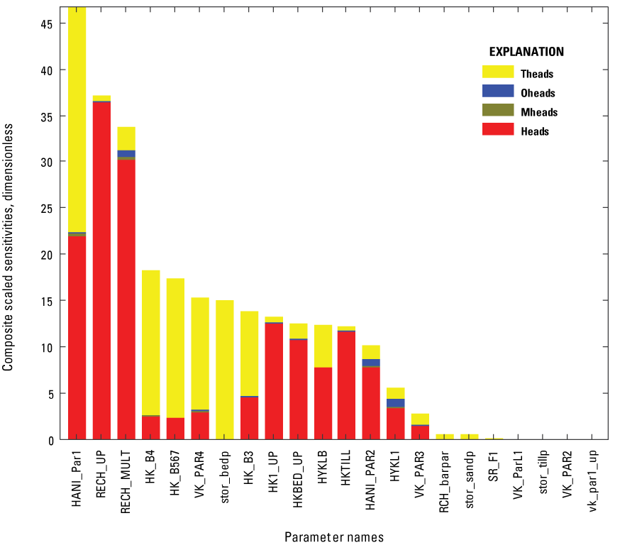
Graph showing composite scaled sensitives (CSS) of parameters to observation datasets for the transient short-term pump test simulation (SPT) of December 2010, area-wide model, Savage Municipal Water-Supply Superfund site, Milford, New Hampshire. Parameters are listed in table 3. theads, transient heads from monitoring wells; oheads, steady-state heads from observation wells (unconsolidated aquifer); mheads, steady-state heads from bedrock monitoring wells; heads, steady-state heads from residential water wells.
The steady-state December 2010 simulation includes observations from river seepage (Harte and others, 1997). Valley recharge (parameter RECH_MULT) has the highest CSS indicating that valley recharge is the most informed parameter by the river observations used in this simulation. Figure 7 shows an example of typical CSS results from a steady-state December 2010 simulation. Upland recharge (parameter RECH_UP) and bedrock anisotropy (parameter HANI_Par1) are the most informed by residential heads (water levels).
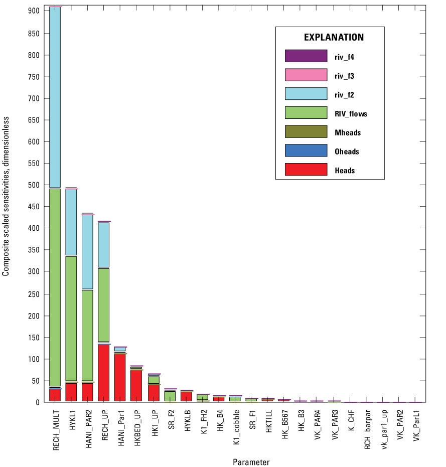
Graph showing composite scaled sensitives (CSS) of parameters to observation datasets for the steady-state simulation of early December 2010 (D2010). Parameters are listed in table 3. mheads, steady-state heads from bedrock monitoring wells; oheads, steady-state heads from observation wells (unconsolidated aquifer); heads, steady-state heads from residential water wells; riv_f4, weight applied to streamflows at Hartshorn Brook; riv_f3, weight applied to streamflows near the Milford Fish Hatchery withdrawal wells; riv_f2, weight applied to streamflows at Tucker Brook; RIV_flows, weight applied to streamflows on the Souhegan River by P2 and main stem (MS) 2, and by tributary 1; explanation of parameter names provided in table 3; river reaches are shown on figure 1.1.
Calibration Results
There are three simulation sets in this report (long-term mean annual, December 2010, and short-pump test). In discussing the simulation, different parameter variations are presented other than the calibrated version in order to highlight parameter sensitivity. The calibrated version per simulation set is always referred to as the calibrated simulation or base simulation for either long-term mean annual, December 2010, and short-pump test (Harte and Watt, 2021).
The long-term mean annual simulations were preliminary in nature and focused on bulk adjustments of hydraulic properties (kh, kv), recharge, and river properties (stage, bed, and hydraulic conductance). Layers were kept homogeneous, horizontally isotropic, and vertically anisotropic. Results from the long-term mean annual calibrated model indicate that model-computed heads are slightly higher than observed heads at low altitudes but slightly lower than observed heads at high altitudes (fig. 8). The automated calibration yielded a residual mean head difference (observed minus model-computed heads) of –6.3 ft, a median head difference of –1.4 ft, and an absolute mean head difference of 30.6 ft. Parameter estimation computed a kh of 0.154 ft/d for the uppermost bedrock layer and 0.0038 ft/d for the lowermost bedrock layers. Confidence intervals for both values are large (infinity), suggesting high uncertainty in parameter estimation.
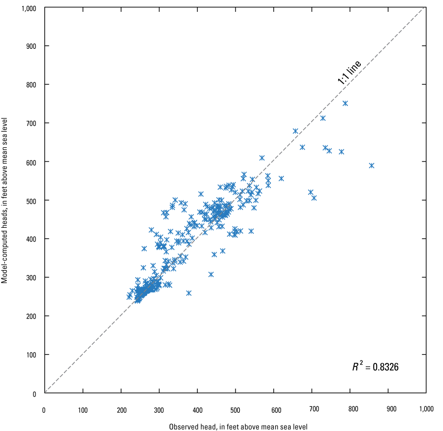
Graph showing observed and model-computed heads from the steady-state, long-term mean annual (LMA) pre-1998 conditions in the area-wide model of the Savage Municipal Water-Supply Superfund site, Milford, New Hampshire. R2, coefficient of determination.
The high uncertainty indicates that additional observation data are needed to constrain parameter estimation and improve the calibration. Parameters from the calibrated model of the long-term mean annual simulations were initially used as input into models of the December 2010 and short-pump test simulations and additional head data were incorporated into the December 2010 simulation. Further, to help the calibration, various levels of heterogeneity and anisotropy were evaluated in a series of simulations to minimize the bias in model-computed heads at high altitudes, as shown by the residuals. The following discussion describes the changes to the short-pump test and December 2010 simulations to evaluate different parameter complexities and improve calibration.
Parameters from the calibrated model of the long-term mean annual simulations were initially used as input into models of the December 2010 and short-pump test simulations. The initial parameter estimates from the calibrated model for the long-term mean annual simulations were used in the short-pump test simulation (called “isotropic, layered homogeneous”; table 4). Heterogeneity was incorporated into the model by interpolating hydraulic conductivities, calculated from the packer hydraulic tests (Weston Solutions, Inc., 2010) between wells.
Table 4.
Comparison of model-computed and observed heads from selected bedrock wells for the short-term pump test at the Savage Municipal Water-Supply Well Superfund site, Milford, New Hampshire.Head residuals (observed minus model-computed heads) for horizontal isotropic conditions, either layered homogeneous or heterogeneous, are large (table 4). When horizontal anisotropy in kh was incorporated into the model at a ratio of 20:1 (short-pump test-anisotropic heterogeneous simulation) in the row (y) to column (x) direction to approximate preferential flow along the prevalent fracture strike, head residuals greatly decreased. Head residuals changed by relatively small amounts when incorporating heterogeneity into the model from the packer hydraulic test data. Results of the short-pump test simulations indicate that horizontal anisotropy is one of the most important parameters controlling flow in the bedrock.
Anisotropy ratios of 10:1 and 20:1 (y to x direction) produce an elongated potentiometric head contour that extends to the northeast as a result of withdrawals at well BR–6. The heads are shown in figure 9A for the contour at 240 ft altitude above msl for model layer 4 (bedrock layer 2) at the end of short-pump test simulation (simulations identified in table 4 as isotropic and homogeneous, and anisotropic and heterogeneous). The 240-ft contour is a representative contour that illustrates the variations in model-computed heads when compared with results from multiple simulations. Simulations presented highlight differences between isotropic and anisotropic conditions. Model-computed heads from other model layers (layers 5, 6, and 7) show greater drawdown than the other layers and model-computed heads show that simulated heads vary based on the kh for those layers. The observed heads, where water levels were measured, are labeled next to the monitoring well (fig. 9A).
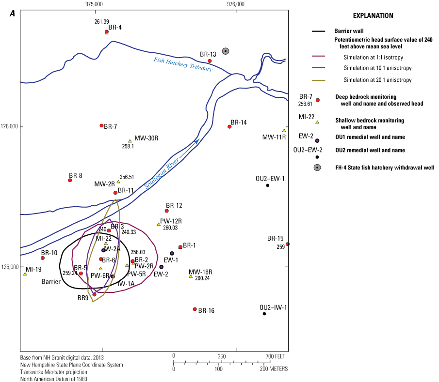
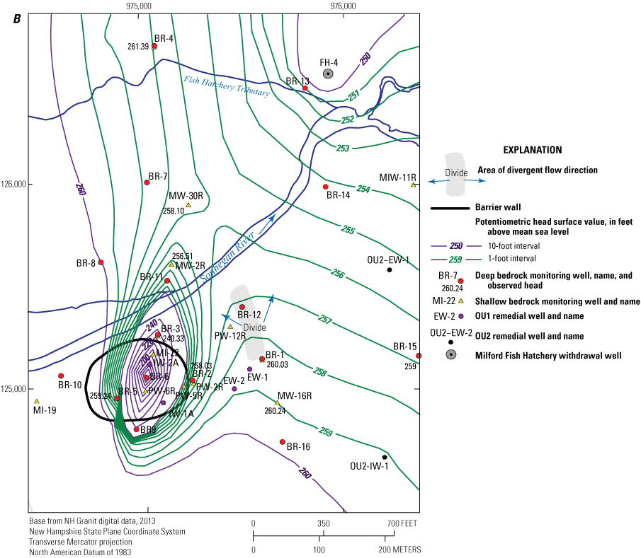
Maps showing contours of model-computed potentiometric heads by well BR–6 in bedrock layer 2 (model layer 4) for the transient short-term pump test (SPT), December 2010, and observed heads in selected bedrock wells, for A, the 240-foot potentiometric head contour for selected simulations, and B, for 1-foot-potentiometric-head-contours calibrated model from the calibrated SPT simulation, area-wide model, Savage Municipal Water-Supply Superfund site, Milford, New Hampshire. OU, operable unit.
Iterative calibration between the short-pump test and December 2010 simulations indicated that, at an anisotropy of 20:1 ratio (y to x direction), head residuals were larger than using a 10:1 ratio for the December 2010 simulations alone. The final calibrated model for the December 2010 and short-pump test simulations, which uses an anisotropy of 10:1, shows that, at the end of the short-pump test simulation, a groundwater divide forms near bedrock well BR–1. At the divide, flow diverges to the west back to the withdrawal well (BR–6) and to the east following the valley-wide direction of flow (fig. 9B). The location of the divide is beneficial in that it contains contaminants in the bedrock underlying OU1 from lateral transport to the east. The distribution of observed heads also corroborates that a divide forms in this area.
The calibrated results with a fully anisotropic heterogeneous model for the December 2010 simulation show an improvement in model fit (fig. 10) and less altitudinal bias compared with the long-term mean annual simulation (fig. 8). Model-computed heads in the December 2010 simulation match observed heads better at high altitudes (more than 700 ft above msl) unlike the long-term mean annual simulation. The automated calibration yielded a mean head difference (between observed and model-computed heads) of 14.5 ft, a median head difference of 3.7 ft, and an absolute mean head difference of 34.1 ft.
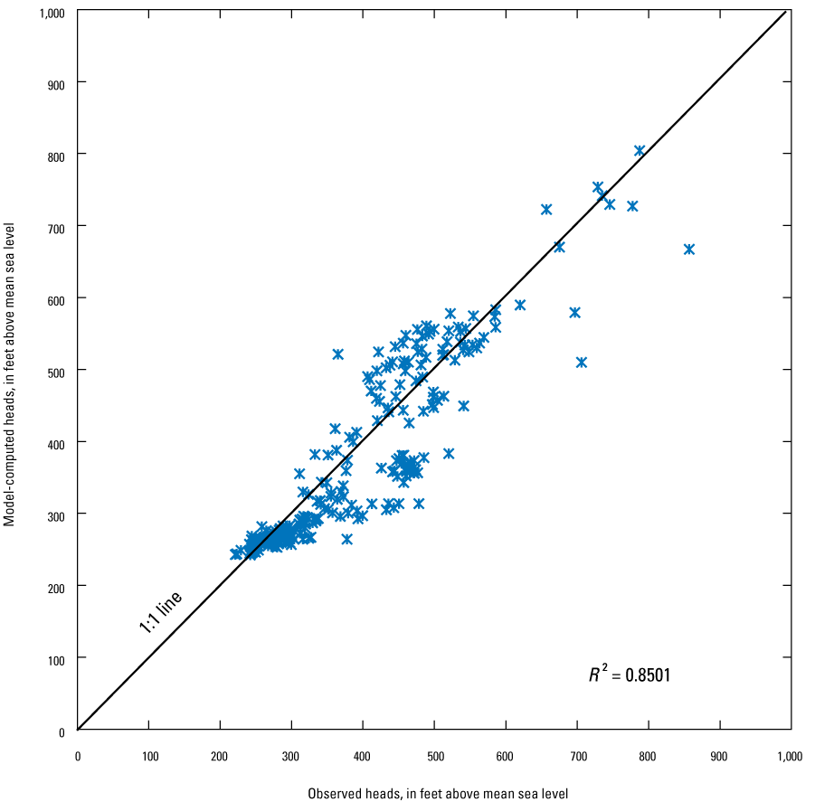
Graph showing observed and model-computed heads from the calibrated steady-state simulation for early December 2010 (D2010) conditions, area-wide model, Savage Municipal Water-Supply Superfund site, Milford, New Hampshire. R2, coefficient of determination.
Model-computed river seepage in the December 2010 simulation model matches well (relative percent difference of –2; table 5) with the observed river seepage for the second reach of the main stem (MS2) of the Souhegan River (app. 1). Model-computed river seepages for several tributaries match poorly (table 5). Less weight was applied in matching simulated to observed river seepages for the tributaries because of smaller flows.
Table 5.
River seepage of selected stream reaches from the calibrated model for steady-state simulation of early December 2010 conditions, Savage Municipal Water-Supply Well Superfund site, Milford, New Hampshire.From Harte and others (1997).
Parameters were estimated using a multiplicative factor to the heterogeneity distribution derived from the packer hydraulic test (Weston Solutions, Inc., 2010) and adjusted for rock type and altitude. The kh in areas underlying land surface altitudes more than 330 ft was set less than the kh less than 330 ft. The range in kh specified in the final models for December 2010 (and short-pump test) simulations is provided in table 6.
Table 6.
Final horizontal hydraulic conductivity for the area-wide model, December 2010 steady-state conditions, Savage Municipal Water-Supply Well Superfund site, Milford, New Hampshire.The uncertainty in parameter estimates are generally large (several orders of magnitude), indicating that model reliability could be improved with additional transient head and seepage data. In particular, river seepage data in upland areas would provide considerable leverage to constrain model parameterization.
Model-computed potentiometric heads in the bedrock for the calibrated December 2010 simulation model range from approximately less than 240 ft to more than 810 ft above msl (fig. 11). In the Milford-Souhegan River Valley, the potentiometric heads in the bedrock follow a similar pattern as do the heads in the MSGD aquifer as identified by Harte and others (1997). The head residuals are visible in figure 11 as a range of colors at wells with available water-level data; spatial bias is visible as a clustering of similar colors. Some clusters of similar colors occur in several areas, indicating head residuals differ by a similar amount; additional spatial parameterization of the bedrock kh could be incorporated into the model to help improve calibration. An area with large head residual occurs at the southeastern corner of the model (fig. 11).
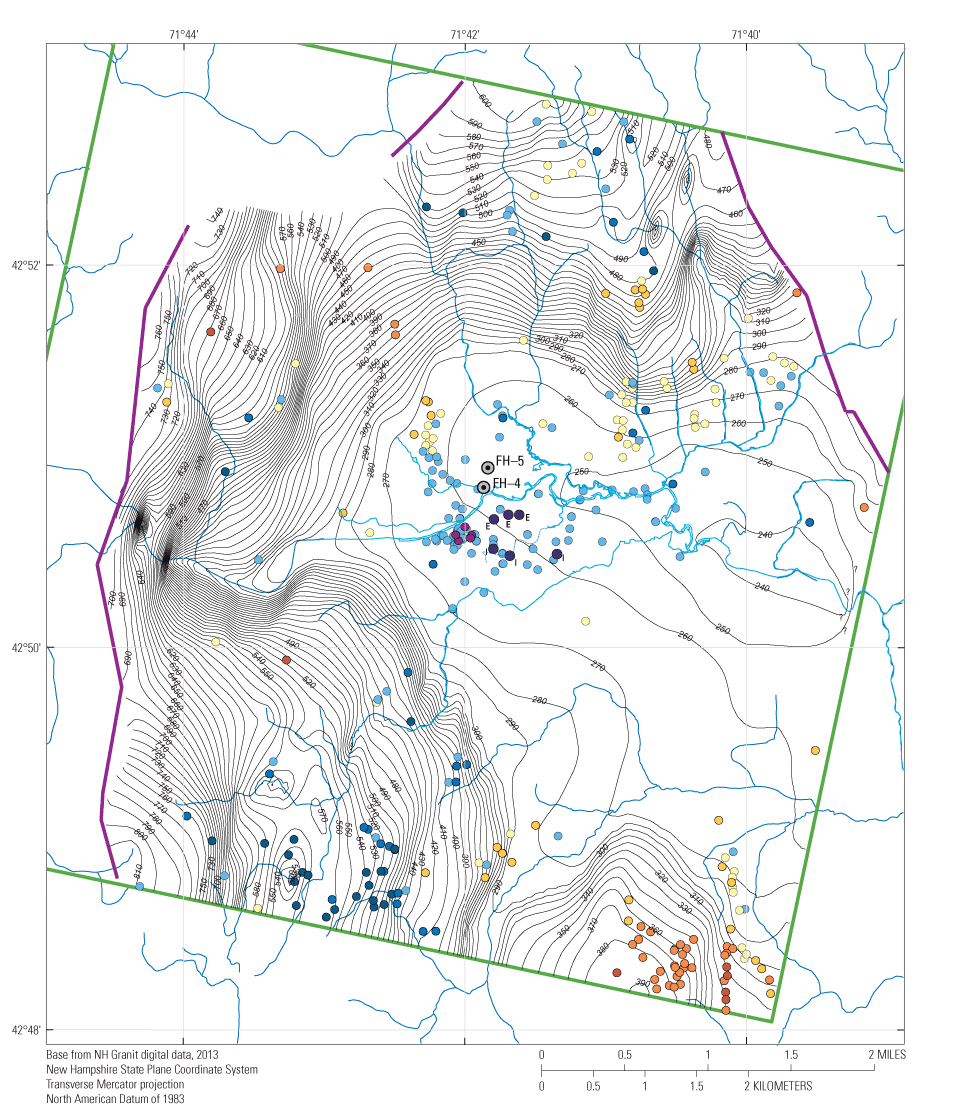
Map showing model-computed potentiometric-head contours from bedrock layer 2 (model layer 4) of the calibrated steady-state simulation of early December 2010 (D2010) conditions and head residuals from observations, Savage Municipal Water-Supply Superfund site, Milford, New Hampshire. OU1 is the primary source area of tetrachloroethylene (PCE) and OU2 is the extended plume area of PCE for the Savage Municipal Water-Supply Well Superfund site.
Model-computed heads in the valley for the calibrated December 2010 simulation model tend to be slightly higher than observed heads by 3 to 5 ft. Given that model-computed river seepage for the main-stem Souhegan River matches observed seepage, which is indicative that simulated rates of recharge in the valley are reasonable, it is possible that the hydraulic conductivity of the bedrock and unconsolidated sediments could be further refined in the valley to improve the calibration.
Model Testing
The model parameters were tested by simulating a second aquifer test of well BR–6 that was completed in April 2013 (Weston Solutions, Inc., 2013). The pump rates were similar to those from the short-pump test simulation, but the April 2013 test lasted several more days (total test time 9.5 days). The April 2013 aquifer test (called the extended test) was simulated using parameters from the calibrated short-pump test simulation model. For the extended test, simulated drawdowns stabilized and did not further decrease, similar to observed drawdowns from monitoring wells. The primary lesson learned about the flow system from the extended test is that the storage properties of the bedrock and adjacent boundary conditions appear to be reasonably approximated in the area-wide model. A storage coefficient of 0.00009 was used for all bedrock layers. Storage coefficients of 0.03 and 0.003 were used for the sand and gravel and the till units, respectively. The specified storage coefficient for the sand and gravel unit represents a thickness–based, proportionally averaged value between specific yield and storage coefficient, which is comparable to values reported in Harte (1997).
As part of the extended test at well BR–6, unique tracers were applied to adjacent bedrock monitoring wells (BR–2, BR–3, BR–12, and MW–2R; fig. 9) to identify transport pathways to well BR–6 (Weston Solutions, Inc., 2013). Emplacement of unique tracers at each of the four spiked wells allowed for the ability to identify the transport and origin of the tracer. Tracers were detected in pumped waters at well BR–6 from all wells except well MW–2R, which is a shallow-bedrock well across the river from well BR–6. A range of velocities was calculated from first arrival times reported by Weston Solutions, Inc. (2013). Velocities are faster oblique to fracture strike or parallel to fracture strike than orthogonal to fracture strike (updip; table 7).
Table 7.
Tracer first arrival times and calculated hydraulic parameters from adjacent bedrock monitoring wells from the April 2013 aquifer test at well BR–6, Savage Municipal Water-Supply Well Superfund site, Milford, New Hampshire.[—, no data]
Horizontal hydraulic conductivities (kh) were calculated based on the following one-dimensional equation based on Darcy’s law and substitution of velocities from tracer arrivals:
whereBulk kh and discrete fracture kh were calculated by using bulk rock and fracture specific porosities, respectively (table 7). The bulk rock porosity integrates unfractured and fractured volumes of the rock. A bulk rock porosity of 0.001 is equivalent to a 1/8-inch fracture aperture (approximately 0.01 ft) opening every 10 ft of rock thickness. A fracture porosity accounts for the fracture only, and a porosity of 0.5 assumes that the fracture surface is not perfectly planar and that some parts of the fracture surfaces are in contact with one another. To bracket estimated kh from diffuse flow (bulk rock) and fracture flow, both porosities are specified. For arrival time through flow in a fracture, a calculated kh based on equation 1 must be higher than a kh derived from an arrival time through the bulk rock.
The kh values estimated from tracer velocities for the bulk rock are comparable to the higher range of kh values in the model for bedrock layer 2 (table 6). The similarity between high values of model-derived kh and tracer estimates of kh is reasonable given that first arrivals of tracers will be controlled by the kh of high kh zones in the rock and suggests that the calibrated model provides reasonable estimates of kh. The maximum kh estimated from packer hydraulic test data (Weston Solutions, Inc., 2013) identified the most permeable fractures at well BR–2 (0.34 ft/d per ft of rock) compared with wells BR–12 (0.16 ft/d per ft of rock) and BR–3 (0.03 ft/d per ft of rock). However, the connectivity of the fractures is such that well BR–6 preferentially withdraws groundwater along the prevalent strike (northeastern) direction toward well BR–3. The kh values estimated from tracer velocities assuming flow in fractures are much higher than estimates of kh for the bulk rock (table 7).
Flow Path Analysis Simulations
Advective transport was simulated for the calibrated December 2010 model (base) and other modifications of the December 2010 model as described below, including selected parameter adjustments based on parameter uncertainty, hydrologic conditions such as recharge, and various scenarios such as changes in remedial operations. Advective transport is derived from the average interstitial flow of groundwater and does not include processes of dispersion, retardation, or matrix diffusion that affect PCE transport. The particle-tracking postprocessing software MODPATH (Pollock, 1994) was used.
The area-wide model approximates the bulk hydraulic properties of the fractured bedrock through an equivalent porous media representation. Discrete fracture connectivity is not simulated but implicitly incorporated into the bulk properties of the model. Advective transport (in the form of pathlines generated from models) is controlled by heads, bulk hydraulic properties, and porosity (which affects velocity). The model approximates transport because it does not explicitly simulate discrete fractures. Therefore, pathlines can be viewed as potential pathways dependent on fracture connectivity. Tetrachloroethylene (PCE) solute transport that follows the advective transport trajectory could be attenuated to low concentrations before the pathlines terminate at their final discharge location. Consequently, the pathlines presented in this report represent the maximum potential extent of PCE transport for that specified simulation.
Advective transport is simulated by forward tracking particles (points specified within the groundwater-flow model) from areas of contaminated bedrock layers (all bedrock layers). The extent of the contaminated bedrock layers is based on the 1,000-microgram per liter (µg/L) contour value of PCE concentrations (fig. 1; Weston Solutions, Inc., 2010; Burton and Harte, 2013, fig. 1). Particles were placed along the 1,000-µg/L contour value and forward tracked in December 2010 simulations (December 2010 calibrated model and variations thereof) to generate the model-computed pathlines.
Porosity was kept uniform within each modeled unit. Porosity of the sand and gravel and till was kept at 0.3 and the bedrock at 0.00000254. This low porosity for the bedrock was based on a fracture frequency of one fracture every 16 ft and estimated aperture of 0.039-inch of fractures divided by the bedrock thickness. Porosity affects velocity calculations only.
Particles are allowed to terminate at their final discharge location regardless of travel times. Travel times are difficult to quantify in fractured systems using an equivalent porous medium approach because of differences in advective transport in fractures and the bulk rock.
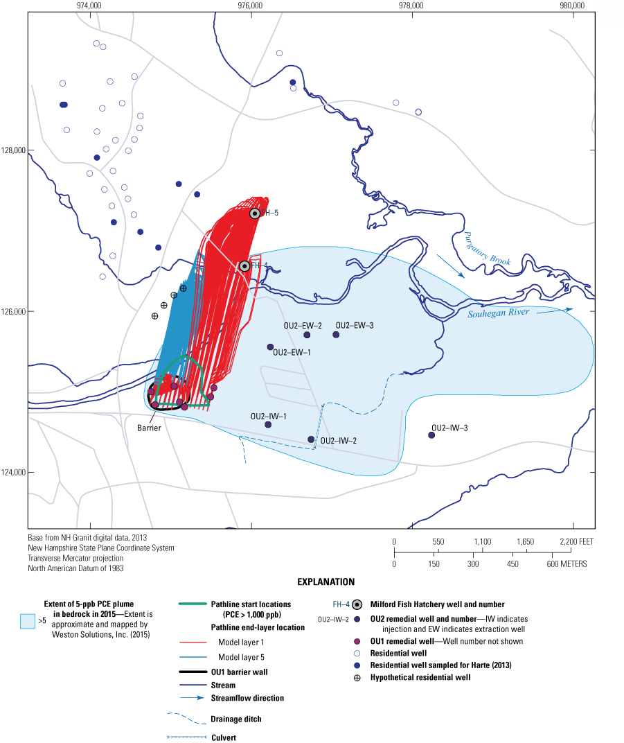
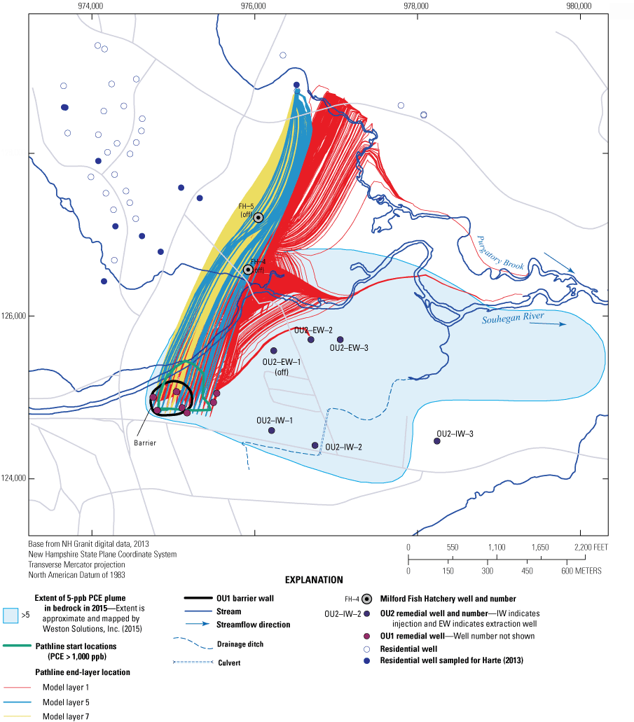
Pathlines from particle tracking are projected onto a two-dimensional surface from all model layers for the base December 2010 model (fig. 12, at back of report) and modifications to the December 2010 model for parameter/scenario evaluations. Path line illustrations for parameter and scenario evaluations are shown in figures 13 through 17 (at back of report). The calibrated December 2010 model is termed the base case for advective transport of particles. Pathlines are color coded to show their final discharge location (endpoint) per model layer. For the base case (fig. 12, at back of report) and for the other scenario evaluations (figs. 13–17, at back of report), the observed extent of the PCE plume in the bedrock, as mapped to the 5 µg/L concentration contour by Weston Solutions Inc. (2015), is shown as a reference. Model-computed pathlines within the observed extent are interpreted as more likely to occur than pathlines outside the observed extent.
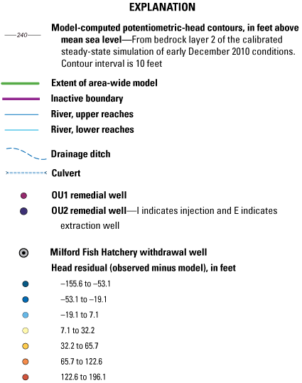
Map showing maximum potential pathlines forward tracked from areas with contaminated groundwater, calibrated model, steady-state simulation of early December 2010 conditions (D2010), area-wide model, Savage Municipal Water-Supply Superfund site, Milford, New Hampshire. D2010, steady-state simulation of early December 2010 conditions; PCE > 1,000 ppb, tetrachloroethylene greater than 1,000 parts per billion.
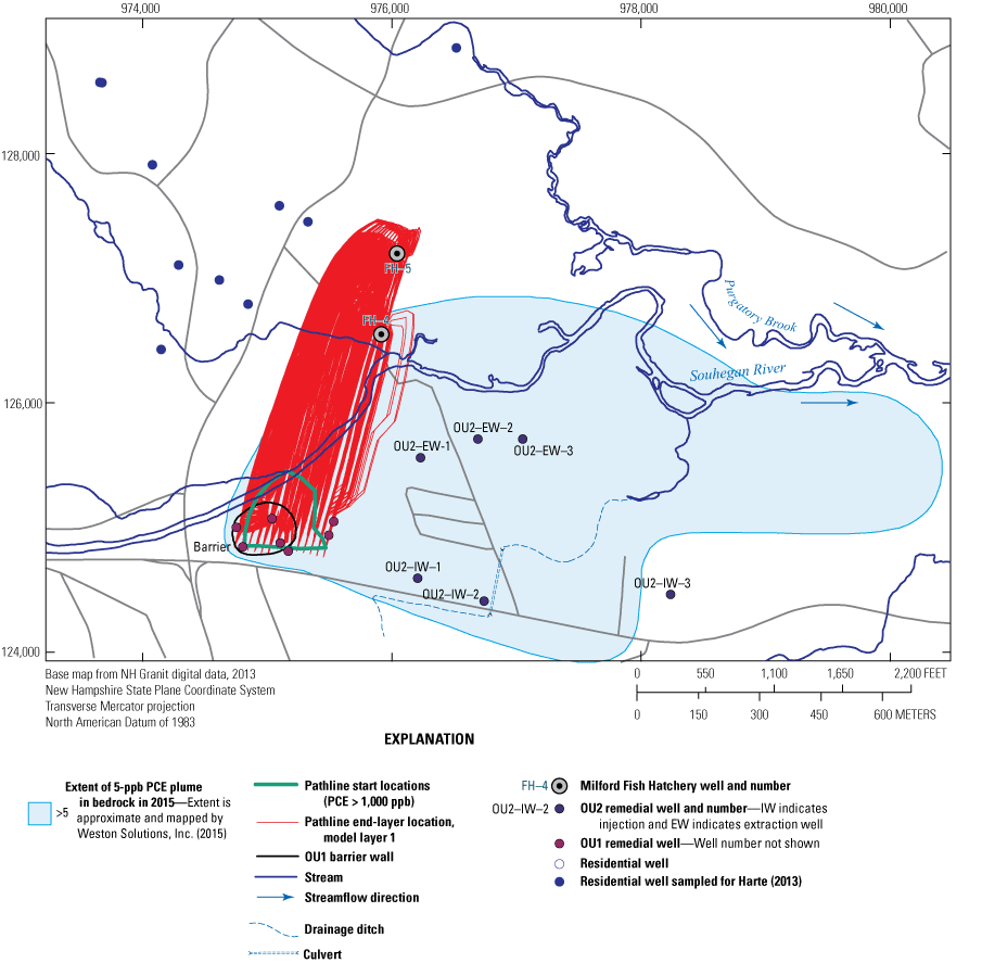
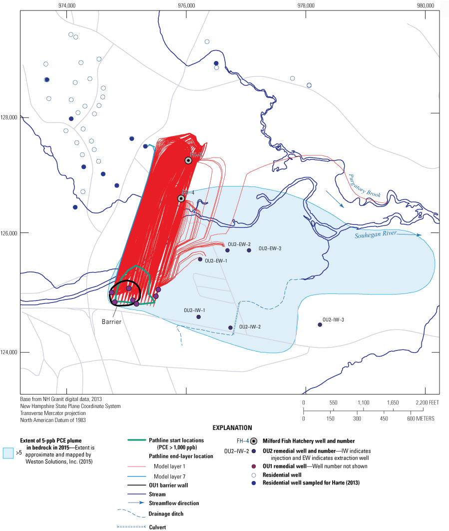
Map showing maximum potential pathlines forward tracked from areas with contaminated groundwater from a simulation with no anisotropy specified in the crystalline-rock aquifer for the steady-state simulation of early December 2010 (D2010) conditions, area-wide model, Savage Municipal Water-Supply Superfund site, Milford, New Hampshire. PCE > 1,000 ppb, tetrachloroethylene greater than 1,000 parts per billion.
Map showing maximum potential pathlines forward tracked from areas with contaminated groundwater from a simulation with the addition of hypothetical residential water-supply wells for the steady-state simulation of early December 2010 (D2010) conditions, area-wide model, Savage Municipal Water-Supply Superfund site, Milford, New Hampshire. PCE > 1,000 ppb, tetrachloroethylene greater than 1,000 parts per billion.
Map showing maximum potential pathlines forward tracked from areas with contaminated groundwater from a simulation with the hypothetical termination of withdrawals at Milford Fish Hatchery withdrawal wells for the steady-state simulation of early December 2010 (D2010) conditions, area-wide model, Savage Municipal Water-Supply Superfund site, Milford, New Hampshire. PCE > 1,000 ppb, tetrachloroethylene greater than 1,000 parts per billion.
Map showing maximum potential pathlines forward tracked from areas with contaminated groundwater from a simulation with increase withdrawals at well OU2–EW1 for early December 2010 (D2010) conditions, area-wide model, Savage Municipal Water-Supply Superfund site, Milford, New Hampshire. PCE > 1,000 ppb, tetrachloroethylene greater than 1,000 parts per billion; OU2–EW1, extraction well 1 for OU2 remedial system.
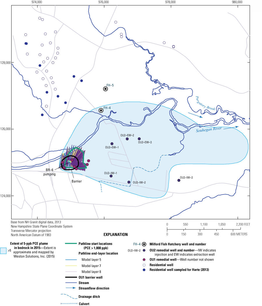
Map showing maximum potential pathlines forward tracked from areas with contaminated groundwater from a simulation with a continuous withdrawal at well BR–6 for early December 2010 (D2010) conditions, area-wide model, Savage Municipal Water-Supply Superfund site, Milford, New Hampshire. PCE > 1,000 ppb, tetrachloroethylene greater than 1,000 parts per billion.
The base case shows most pathlines travel in the crystalline rock and upwardly discharge near the Milford Fish Hatchery withdrawal wells in the MSGD aquifer (fig. 12, at back of report). A few pathlines (not visible) are captured by extraction of the existing OU1 remedial wells in the MSGD aquifer. All pathlines discharge to extraction wells in layer one of the model. The combination of preferred anisotropy in the northeastern direction in the bedrock and large withdrawals at the Milford Fish Hatchery withdrawal wells in the MSGD aquifer (table 2) creates a preferential transport to areas by the Milford Fish Hatchery withdrawal wells. In contrast, advective and solute transport of PCE in the MSGD aquifer indicates a predominantly easterly path and less pathlines discharge to the Milford Fish Hatchery withdrawal wells from the OU1 area (Harte and others, 1999; Harte, 2004). The observed PCE in the bedrock also shows an easterly transport pathway suggesting several alternate pathways including (1) a possible west-east fracture network, (2) alternate PCE source areas, and (3) communication and transport between the bedrock and the MSGD aquifer.
Alternative Conceptualization of the Crystalline-Rock Aquifer
Fracture length is an important control on flow in the bedrock aquifer and is an unknown variable. Fractures that truncate without intersecting an adjacent fracture would result in low permeability zones with little flow. To simulate finite fracture length, a simplified adjustment was made to the model where the anisotropy in the model was decreased by a factor of 100 for every 20th model row, or approximately 1,400 ft over the area-wide model. Simulated pathlines (not shown) moved to the northeast as in the base case but in a convex pattern, coinciding with the low anisotropy row where the fracture was hypothesized to terminate. At fracture terminal locations, pathlines moved upward, which would ultimately result in additional upward discharge to the sand and gravel and till units at fracture terminal locations and a corresponding decrease in groundwater flow in the bedrock. It is likely that many fractures terminate at cross-cutting connections with other fractures, which would cause sharp angular pathlines to form instead of upflow. Nevertheless, this simplified modification helps illustrate the importance of fracture lengths on flow.
Horizontal anisotropy, as shown in simulations of short-pump test, is a major control on flow in the crystalline-rock aquifer. Simulations with and without anisotropy show a distinctly different pattern of pathlines (figs. 12 and 13, at back of report). Without anisotropy, many pathlines discharge to tributaries to the Souhegan River farther east in the valley (fig. 13, at back of report) than in the base case (fig. 12, at back of report).
Changes in Hydrologic Conditions
Adjusting recharge rates by ±50 percent from the base case has a small effect on pathlines (not shown) that were forward tracked from PCE-contaminated areas underlying OU1. The general path line trajectory and patterns look similar to the base case, particularly for the high recharge model. However, low recharge causes some pathlines to move to the west by 100 ft, which puts the projection of the pathlines for the low recharge simulation closer to some residential water wells than pathlines for the base case. Recharge from the upland areas west of the residential water wells is likely an important control on limiting the northwestern transport of contaminated PCE from OU1.
Changes in Well Withdrawals
Several simulations were completed where well withdrawals were adjusted based on potential future scenarios. Scenarios included increased residential development and withdrawals at new residential water-supply wells, cessation of withdrawals at the Milford Fish Hatchery withdrawal wells, increase in withdrawals at OU2 (OU2–EW1 well), termination of remedial operation in OU1 and OU2, and initiation of a pump and treat remedy in the crystalline-rock aquifer underlying OU1.
The addition of new residential water-supply wells north and near the river affects advective transport of PCE contaminants. A scenario where four new hypothetical residential water wells were added to the base case was completed to represent the potential expansion of housing in that area (fig. 14, at back of report). The wells were simulated to depths of 400 ft bls and withdrawals were specified at rates similar to other residential water wells. For this scenario, some of the pathlines forward-tracked from contaminated areas discharge to the hypothetical residential water wells. The remaining pathlines either discharge to the Milford Fish Hatchery withdrawal wells or discharge to the remedial wells in OU1. Depending on the proportion of noncontaminated to contaminated PCE groundwater discharging to the hypothetical residential water wells, PCE concentrations in some wells could exceed maximum contaminant levels.
The hypothetical cessation of withdrawals at the Milford Fish Hatchery withdrawal wells (as of 2013 withdrawals were approximately 1,800 gal/min) causes some pathlines to discharge farther north toward residential water wells in the bedrock. Some pathlines discharge near tributaries to the north near high-yielding residential water wells in this area, whereas others discharge to the Souhegan River to the east (fig. 15, at back of report). A few pathlines discharge to remedial extraction wells in OU2. The overall pattern of pathlines is complex and is affected by multiple hydrologic sinks (withdrawal wells and discharge to rivers).
The hypothetical termination of remedial injections and extractions at OU1 and OU2 has a small effect on pathlines (not shown). For this scenario, pathlines show similar movement as in the base case excluding the pathlines that discharge to the Milford Fish Hatchery withdrawal wells, which formerly were captured by OU1 remedial extraction wells in the base case.
Increasing the rates of extraction at remedial wells in OU2 at EW–1 from 0 to 125 gal/min causes some pathlines to discharge to OU2 extraction wells (EW–1 and EW–2). Further, it has a ripple effect and causes a decrease in flow velocities by the Milford Fish Hatchery withdrawal wells that allows the partial capture of pathlines at one of the residential water wells (fig. 16, at back of report). However, it should be noted that the interception of one particle pathline to a single residential well is viewed as not strongly supportive of a major shift in flow but rather a minor shift in flow.
The addition of well BR–6 as a long-term (to steady-state conditions) withdrawal well captures almost all pathlines from the contaminated area (fig. 17, at back of report). Pathlines track back toward well BR–6 and no pathlines discharge to the north. Few pathlines discharge to the OU1 remedial wells inside the barrier, instead pathlines are captured by extraction at well BR–6. Results of this simulation indicate that continuous withdrawals at well BR–6 could be effective in preventing or reducing the transport of PCE contamination in the bedrock.
Tetrachloroethylene Transport
PCE transport was simulated to understand the potential effects of flow interactions with the bedrock on PCE concentrations in the MSGD aquifer. PCE transport was simulated with the MSGD model (Harte, 2012), using the Eulerian-Lagrangian localized adjoint method (ELLAM) algorithm for the three-dimensional method-of-characteristics groundwater flow and transport model (MOC3D; Heberton and others, 2000; Konikow and others, 1996) and fluxes apportioned from the area-wide model (calibrated December 2010 model) across the bedrock surface. Fluxes were applied following methods described by Banta and others (2008). Appendix 2 includes additional information on procedures used to apportion flux from the area-wide model to the MSGD-aquifer model. The ability to incorporate fluxes from the area-wide model (called parent model) into the smaller MSGD aquifer model (called target model) allows for a more realistic representation of flow in the basal part of the MSGD aquifer near the bedrock surface.
The MSGD-aquifer model simulates the solute transport of a single species, in the case of this model it is PCE. Dissolved and sorbed mass are accounted for in the model. A detailed explanation of the MSGD-aquifer model and solute transport processes can be found in Harte (2004, 2012). The base simulation case from Harte (2012, table 4) was rerun for this study with the addition of flow across the bedrock surface as computed by the parent model and assigned to the target model. The base model in Harte (2012) was based on proposed, operational, pump-and-treat rates for OU1 and OU2 following conditions described by Harte (2004).
The MSGD model and simulation uses the PCE concentration in 1998 as the starting plume condition and simulates approximately 20 years of PCE attenuation without additional PCE source terms, such as the dissolution of dense nonaqueous phase liquids. Starting conditions in late 1998 are contemporaneous with the installation of the barrier wall. Sources of PCE, outside the barrier wall within the MSGD aquifer in OU1 have not been identified to date based on decreases in PCE concentrations at monitoring wells outside the barrier wall (Weston Solutions, Inc., 2014). Therefore, based on containment of PCE sources, the MSGD-aquifer model satisfactorily reproduces the dissolved, disconnected PCE plume outside the barrier wall. Inside the barrier wall, PCE concentrations are not decreasing (PCE sources are likely present), thus the model should not be used to simulate conditions inside the barrier.
Two simulations were completed with potential end-member PCE concentrations. A PCE concentration of 0 µg/L was assigned to represent upflow of clean groundwater discharging from the bedrock to the basal part of the MSGD aquifer. Another simulation was completed with a PCE concentration of 100 µg/L in the basal part of the MSGD aquifer to represent contaminated groundwater. An upper bedrock groundwater concentration of 100 µg/L is representative of PCE concentrations from the upper bedrock (Weston Solutions, Inc., 2012). The purpose of assigning a 0-µg/L PCE concentration (and load) was to help assess the effect of the mixing of clean water on PCE attenuation in the basal parts of the MSGD aquifer.
Simulated upflow and downflow across the bedrock surface to the active regions of the MSGD aquifer total 0.07 cubic foot per second (ft3/s) and 0.15 ft3/s, respectively. Therefore, the interaction with the bedrock represents a net loss to the MSGD aquifer of 0.08 ft3/s. In comparison, recharge to the MSGD aquifer is 3.3 ft3/s; the net loss of the MSGD to the bedrock represents approximately 3 percent of recharge. Flow across the bedrock surface is volumetrically small relative to other parts of the MSGD water budget. Transport of PCE in the MSGD aquifer is slightly affected by bedrock upflow. The effect of bedrock upflow on PCE transport is particularly small when the PCE plume is relatively large and concentrations high (large mass) in the MSGD aquifer.
Figure 18 shows the changes in mass (dissolved and sorbed) of the PCE plume in the MSGD aquifer over time for the two end-member simulations. The amount of sorbed mass exceeds the dissolved mass because the retardation factor used in the model ranges from 2 to 2.5; a retardation factor of 1 means no retardation and little accumulation of PCE onto sorbed phases. The mass of PCE decreases because of attenuation of the plume primarily from capture of PCE by the remedial extraction wells in OU1 and OU2, and discharge of PCE to the Souhegan River. Before year 10 from the start of simulation (2008), the effect of contaminated bedrock water on the MSGD aquifer is not visible (fig. 18). However, after 2008, a divergence in the computed PCE mass is visible. Given that bedrock upflow (0.07 ft3/s) represents approximately 1 percent of the total inflow (7.7 ft3/s) into the aquifer, the potential load of PCE is low. By 2017 (the end of the simulation) when PCE mass in the MSGD aquifer is small (less than 66.14 pounds [30 kilograms]), the effect of PCE load from contaminated bedrock upflow results in twice the PCE mass in the MSGD aquifer as the simulation assuming no PCE load from bedrock upflow.
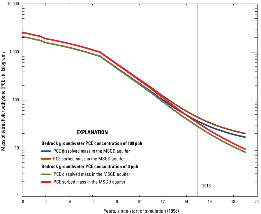
Graph showing mass of tetrachloroethylene (PCE) concentrations (dissolved and sorbed) in the Milford-Souhegan glacial-drift (MSGD) aquifer for simulations of a transport model with and without contaminated PCE from flow across the bedrock surface, as calculated from the area-wide model, Savage Municipal Water-Supply Superfund site, Milford, New Hampshire. Simulations based on Harte (2012, table 4); PCE assigned to the MSGD aquifer model from fluxes apportioned from the area-wide model and assigned PCE concentrations.
Bedrock upflow with contaminated PCE causes a small tailing effect in PCE concentrations in the MSGD aquifer. High concentrations (more than 1,000 ppb) of PCE in the bedrock will cause additional PCE mass to enter the MSGD aquifer. The effect of PCE transport and PCE load from the bedrock to the MSGD aquifer is likely less than the contribution of mass from the till because of high retardation and sorbed mass in the till (Harte, 2012).
Further work can be done to examine the spatiotemporal differences in PCE concentrations from the inclusion of bedrock flow across the bedrock surface, including an examination of linkages between the models for different hydrologic conditions. The procedures and utilities generated by this study and discussed in appendix 2 will help expedite further analysis.
Findings
Simulation of groundwater flow with the area-wide model demonstrates the complex interaction between uplands (more than 330 ft) and valleys in the Milford-Souhegan River Valley. Hillsides adjacent to OU1 affect flow to the residential water wells. The residential water wells also are affected by groundwater flow in the MSGD aquifer. Large withdrawals at the Milford Fish Hatchery withdrawal wells capture a large volume of flow in the bedrock and MSGD aquifer.
Automated calibration results indicate that the model is underconstrained by observed data. To help with underconstrained parameters, selected parameters were eliminated primarily based on CSS rankings (low ranks eliminated). However, additional parameter reductions could be done in the future by eliminating highly correlated parameters using the pcc (parameter correlation coefficients) function of UCODE. The uncertainty of parameters in the model is generally large (several orders of magnitude) except for parameters affected by the aquifer test at well BR–6 (short-pump test) and from river seepage data in the valley areas. River seepage data in upland areas would help refine recharge rates in the uplands and reduce the level of uncertainty in bedrock hydraulic properties.
Calibration of the aquifer test for well BR–6 identified a strong (approximately 10:1) anisotropy in the north-northeastern direction (approximately 15° from true north). Reasonable calibration results were achieved as seen from the simulated cone of depression, which generally matches the observed pattern. Model results also implicitly suggest that the flow system can be approximated with an equivalent porous medium approach for matching of bulk flow in the bedrock. Ranges of model-estimated kh (0.00002 to 0.98 ft/d) were comparable with estimates of bulk rock kh (0.05 to 0.28 ft/d) from observed tracer tests collected during an extended aquifer test at well BR–6 in 2013. Connectivity or preferred anisotropy in the bedrock appears to be more important than heterogeneity. At well BR–6, withdrawals preferentially captured groundwater along the strike of the predominant fracture set and foliation despite a higher kh in a well located updip than wells along the preferential fracture strike. The possibility exists that fractures in the updip direction crop out at the bedrock surface or are truncated by other features.
Advective transport from areas with known PCE contamination by OU1 indicate a preferential transport aligned with the anisotropy of the bedrock. The preferential transport may be enhanced by withdrawals from the Milford Fish Hatchery withdrawal wells in the MSGD aquifer. Although the Milford Fish Hatchery withdrawal wells capture some PCE-contaminated groundwater in many simulations, large withdrawals from the Milford Fish Hatchery withdrawal wells enhance dilution of contaminated groundwater with uncontaminated groundwater. Detection of PCE from pumped waters has not occurred at the well closest to the Souhegan River since 2006 but occurred sporadically before that date, based on samples collected by the NHDES (New Hampshire Department of Environmental Services, written commun., 2006, 2020). The combination of terminating or decreasing withdrawals at Milford Fish Hatchery withdrawal wells, and the additional extraction at OU2 remediation wells may cause an easterly transport of some pathlines.
The linkages established between the area-wide model and the previously developed MSGD aquifer model allow for an improved assessment of PCE transport in the basal parts of the MSGD. The simulations that evaluated the linkage of models showed that bedrock upflow is a small percentage (1 percent) of potential inflow into the MSGD aquifer. However, the PCE load from bedrock upflow to the MSGD aquifer could cause a small tailing effect in PCE concentrations and contribute to prolonging the attenuation of the PCE plume in the MSGD aquifer. Compared to potential variations in retardation factors of the till, the effect of bedrock upflow to the contribution of PCE mass in the MSGD aquifer is likely to be significantly less. Further simulations would be helpful to assess the effect that bedrock upflow and downflow have on PCE mass in the MSGD aquifer; particularly, the inclusion of alternative spatiotemporal patterns of PCE concentrations in simulations.
Implication on the Vulnerability of Residential Water-Supply Wells
Advective transport modeling simulations show that, with the configuration of residential houses and companion residential water-supply wells, as of 2016, capture of PCE by residential water wells appears unlikely for hydrologic conditions typical of 2010. However, simulations also show that adding additional houses and withdrawals from new residential water wells could affect PCE transport. Groundwater withdrawals at other adjacent wells, such as the Milford Fish Hatchery withdrawal wells, could affect advective transport near OU1. Therefore, the potential for future changes in withdrawals should be taken into consideration in the remedial assessment of the site. The development of the area-wide model and linkages established with the MSGD aquifer model should help facilitate any assessments of remediation for the site.
Although not a focus of this study, short (seasonal) and long-term (climatic) changes in hydrologic conditions such as recharge from climate change and variations in streamflow could have an effect on PCE transport. Uniform adjustments in recharge indicated small changes in advective transport, but spatiotemporal (nonuniform) variations may have unforeseen effects.
Summary
In 2010, tetrachloroethylene (PCE), a chlorinated volatile organic compound, was detected in groundwater from deep (more than 300 feet below land surface) fractures in monitoring wells tapping a crystalline-rock aquifer beneath operable unit 1 (OU1) of the Savage Municipal Water-Supply Well Superfund site. Operable units define remedial areas of contaminant concern. OU1 is in the western part of the Milford-Souhegan River Valley. Tetrachloroethylene contamination was previously detected in the overlying glacial sand and gravel deposits and basal till, hereafter referred to as the Milford-Souhegan glacial-drift (MSGD) aquifer, in OU1 and OU2 (western part of the Milford-Souhegan River Valley). Thirty to 40 residential water-supply wells are in close proximity (0.25 mile north) from the PCE-contaminated monitoring wells. Some of the residential water-supply wells are likely installed in similar rock types and formation as those of the monitoring wells. Periodic sampling of residential water-supply wells by the U.S. Environmental Protection Agency and New Hampshire Department of Environmental Services has never detected PCE in groundwater from the residential water-supply wells from the beginning of sampling in 1996 to the present [2020].
Part of assessing the potential for PCE transport involves understanding the movement of groundwater in the crystalline-rock aquifer. One of the tools in understanding movement of groundwater, particularly in complex, highly heterogeneous crystalline-rock aquifers, is the development of numerical models of flow. A numerical groundwater flow model was developed to assess groundwater flow in the crystalline-rock aquifer of the Milford area. The model is called the area-wide model because it encompasses a relatively large area (26.5 square miles). The model consists of 36,966 cells in each of the 8 layers (295,728 total cells) and simulates unconsolidated sediments and approximately 700 feet of the upper bedrock. The model was calibrated by automatic parameter estimation and selective trial and error procedures. Calibration to a short-term pump test in the bedrock yielded a strong, preferential anisotropy of approximately 10:1 in a northeast (row) direction. Model-estimated hydraulic conductivity of the bedrock ranged from 0.000091 to 0.98 ft/d.
Simulations with the area-wide model show that with the 2016 configuration of residential water-supply wells, capture of PCE by the residential water wells appears unlikely for annual hydrologic conditions typical of 2010 based on steady-state, advective transport modeling. However, simulations also indicate that adding residential water wells to the north of the PCE-contaminated monitoring wells could affect the transport of PCE. Groundwater withdrawals at other adjacent wells in the overlying MSGD aquifer could affect advective transport in the crystalline-rock aquifer. Therefore, the potential for future changes in withdrawals in the area, as well as changes in hydrologic conditions including recharge and streamflow, should be considered in the remedial assessment process. The development of the area-wide model and linkages established by this study with the previously developed MSGD aquifer models will help facilitate the development of remedial strategies for this Superfund site.
Selected References
Banta, E.R., Paschke, S.S., and Litke, D.W., 2008, User guide and documentation for five MODFLOW ground-water modeling utility programs: U.S. Geological Survey Techniques and Methods, book 6, chap. A28, 24 p., accessed 2012, at https://doi.org/10.3133/tm6A28.
Bennett, D.S., Lyons, J.B., Wittkop, C.A., and Dicken, C.L., 2006, Bedrock geologic map of New Hampshire, a digital representation of Lyons and others 1997 map and ancillary files: U.S. Geological Survey Data Series 215, 1 CD–ROM, accessed May 3, 2016, at https://doi.org/10.3133/ds215.
Burton, W.C., and Harte, P.T., 2013, Bedrock geology and outcrop fracture trends in the vicinity of the Savage municipal water-supply well superfund site, Milford, New Hampshire: U.S. Geological Survey Open-File Report 2013–1224, 17 p., accessed June 23, 2016, at https://doi.org/10.3133/ofr20131224.
Clark, S.F., Jr., Ferguson, E.W., Picard, M.Z., and Moore, R.B., 1997, Lineament map of area 2 of the New Hampshire bedrock aquifer assessment, south-central New Hampshire: U.S. Geological Survey Open-File Report 96–490, 1 sheet, scale 1:48,000. [Also available at https://doi.org/10.3133/ofr960490.]
Harbaugh, A.W., 2005, MODFLOW–2005, the U.S. Geological Survey modular ground-water model—The ground-water flow process: U.S. Geological Survey Techniques and Methods, book 6, chap. A16, [variously paginated]. [Also available at https://doi.org/10.3133/tm6A16.]
Harbaugh, A.W., and McDonald, M.G., 1996, User’s documentation for MODFLOW–96, an update to the U.S. Geological Survey modular finite-difference ground-water flow model: U.S. Geological Survey Open-File Report 96–485, 56 p. [Also available at https://doi.org/10.3133/ofr960485.]
Harte, P.T., 1997, Preliminary assessment of the lithologic and hydraulic properties of the glacial drift and shallow bedrock in the Mirror Lake area, Grafton County, New Hampshire, U.S. Geological Survey Open-File Report 96–654A, 56 p. [Also available at https://doi.org/10.3133/ofr96654A.]
Harte, P.T., 2004, Simulation of source transport of tetrachloroethylene in ground water of the glacial-drift aquifer at the Savage municipal water-supply well superfund site, Milford, New Hampshire, 1960–2000: U.S. Geological Survey Scientific Investigations Report 2004–5176, 78 p. [Also available at https://doi.org/10.3133/sir20045176.]
Harte, P.T., 2006, Effects of a remedial system and its operation on volatile organic compound-contaminated ground water, operable unit 1, Savage municipal water-supply well superfund site, Milford, New Hampshire, 1998–2004: U.S. Geological Survey Scientific Investigations Report 2006–5083, 80 p. [Also available at https://doi.org/10.3133/sir20065083.]
Harte, P.T., 2010, Hydrostratigraphic mapping of the Milford-Souhegan glacial drift aquifer, and effects of hydrostratigraphy on transport of PCE, operable unit 1, Savage superfund site, Milford, New Hampshire: U.S. Geological Survey Open-File Report 2010–1047, 34 p., 3 pl. [Also available at https://doi.org/10.3133/ofr20101047.]
Harte, P.T., 2012, Evaluation of modeling for groundwater flow and tetrachloroethylene transport in the Milford-Souhegan glacial-drift aquifer at the Savage municipal water-supply well superfund site, Milford, New Hampshire, 2011: U.S. Geological Survey Open-File Report 2012–1079, 29 p. [Also available at https://doi.org/10.3133/ofr20121079.]
Harte, P.T., 2013, Geochemical, isotopic, and dissolved gas characteristics of groundwater in a fractured crystalline-rock aquifer, Savage municipal water-supply well superfund site, Milford, New Hampshire, 2011: U.S. Geological Survey Open-File Report 2013–1089, 25 p., accessed December 2014, at https://doi.org/10.3133/ofr20131089.
Harte, P.T., and Kiah, R.G., 2009, Measured river leakages using conventional streamflow techniques—The case of Souhegan River, New Hampshire, USA: Hydrogeology Journal, v. 17, no. 2, p. 409–424. [Also available at https://doi.org/10.1007/s10040-008-0359-1.]
Harte, P.T., and Mack, T.J., 1992, Geohydrology of, and simulation of groundwater flow in, the Milford-Souhegan glacial-drift aquifer, Milford, New Hampshire: U.S. Geological Survey Water-Resources Investigations Report 91–4177, 75 p., 3 apps. [Also available at https://doi.org/10.3133/wri914177.]
Harte, P.T., and Watt, M.K, 2021, MODFLOW–2005, MODPATH, and MOC3D used for groundwater flow simulation, pathlines analysis, and solute transport in the crystalline-rock aquifer in the vicinity of the Savage Municipal Water-Supply Well Superfund site, Milford, New Hampshire: U.S. Geological Survey data release, https://doi.org/10.5066/F7J102FK.
Harte, P.T., and Winter, T.C., 1995, Simulations of flow in crystalline rock and recharge from overlying glacial deposits in a hypothetical New England setting: Ground Water, v. 33, no. 6, p. 953–964. [Also available at https://doi.org/10.1111/j.1745-6584.1995.tb00041.x.]
Harte, P.T., Flynn, R.J., and Mack, T.J., 1999, Construction and calibration of numerical ground-water-flow models of the western half of the Milford-Souhegan glacial-drift aquifer, Milford, New Hampshire: U.S. Geological Survey Open-File Report 99–462, 76 p. [Also available at https://doi.org/10.3133/ofr99462.]
Harte, P.T., Flynn, R.J., Kiah, R.G., and Severance, T., and Coakley, M.F., 1997, Information on hydrologic and physical properties of water to assess transient hydrology of the Milford-Souhegan glacial-drift aquifer, Milford, New Hampshire: U.S. Geological Survey Open-File Report 97–414, 96 p. [Also available at https://doi.org/10.3133/ofr97414.]
Heberton, C.I., Russell, T.F., Konikow, L.F., and Hornberger, G.Z., 2000, A three-dimensional finite-volume Eulerian-Lagrangian localized adjoint method (ELLAM) for solute-transport modeling: U.S. Geological Survey Water-Resources Investigations Report 00–4087, 63 p. [Also available at https://water.usgs.gov/nrp/gwsoftware/moc3d/moc3d.html.]
Hill, M.C., 1990, Preconditioned conjugate-gradient 2 (PCG2), a computer program for solving ground-water flow equations: U.S. Geological Survey Water-Resources Investigations Report 90–4048, 25 p. [Also available at https://doi.org/10.3133/wri904048.]
Hill, M.C., and Tiedeman, C.R., 2007, Effective groundwater model calibration, with analysis of data, sensitivities, predictions, and uncertainty: New York, Wiley and Sons, 464 p. [Also available at https://doi.org/10.1002/0470041080.]
Hsieh, P.A., and Freckleton, J.R., 1993, Documentation of a computer program to simulate horizontal-flow barriers using the U.S. Geological Survey modular three-dimensional finite-difference ground-water flow model: U.S. Geological Survey Open-File Report 92–477, 32 p. [Also available at https://water.usgs.gov/nrp/gwsoftware/modflow2000/ofr92_477_HFB.pdf.]
Konikow, L.F., Goode, D.J., and Hornberger, G.Z., 1996, A three-dimensional method of characteristics solute-transport model (MOC3D): U.S. Geological Survey Water-Resources Investigations Report 96–4267, 87 p. [Also available at https://doi.org/10.3133/wri964267.]
Koteff, C., 1970, Surficial geologic map of the Milford quadrangle, Hillsborough County, New Hampshire: U.S. Geological Survey Geologic Quadrangle 881, scale 1:62,500. [Also available at https://doi.org/10.3133/gq881.]
Mabee, S.B., and Hardcastle, K.C., 1997, Analyzing outcrop-scale fracture features to supplement investigations of bedrock aquifers: Hydrogeology Journal, v. 5, no. 4, p. 21–36. [Also available at https://doi.org/10.1007/s100400050106.]
Mack, T.J., 2009, Assessment of ground-water resources in the seacoast region of New Hampshire: U.S. Geological Survey Scientific Investigations Report 2008–5222, 188 p. [Also available at https://doi.org/10.3133/sir20085222.]
McDonald, M.G., and Harbaugh, A.W., 1988, A modular three-dimensional finite-difference ground-water flow model: U.S. Geological Survey Techniques of Water-Resources Investigations, book 6, chap. A1, 586 p. [Also available at https://doi.org/10.3133/twri6a1.]
Melvin, R.L., deLima, V.A., and Stone, B.D., 1992, The stratigraphy and hydraulic properties of tills in southern New England: U.S. Geological Survey Open-File Report 91–481, 51 p. [Also available at https://doi.org/10.3133/ofr910481.]
Moore, R.B., Schwarz, G.E., Clark, S.F., Jr., Walsh, G.J., and Degnan, J.R., 2002, Factors related to well yield in the fractured-bedrock aquifer of New Hampshire: U.S. Geological Survey Professional Paper 1660, 51 p. [Also available at https://doi.org/10.3133/pp1660.]
New Hampshire Department of Environmental Services, [undated], Water use registration and reporting program: New Hampshire Department of Environmental Services web page, accessed December 19, 2014, at https://des.nh.gov/organization/divisions/water/dwgb/dwspp/wurrp/index.htm.
Granit, N.H., 2012, Granit data discovery tool: University of New Hampshire database, accessed March 2012 at http://www.granit.unh.edu/data/search?dset=nhhd/nhhd01040001.
Poeter, E.P., Hill, M.C., Banta, E.R., Mehl, S., and Christensen, S., 2005, UCODE_2005 and six other computer codes for universal sensitivity analysis, calibration, and uncertainty evaluation: U.S. Geological Survey Techniques and Methods, book 6, chap. A11, 283 p. [Also available at https://doi.org/10.3133/tm6a11.]
Pollock, D.W., 1994, User’s guide for MODPATH/MODPATH–PLOT, version 3—A particle-tracking post-processing package for MODFLOW, the U.S. Geological Survey finite-difference ground-water flow model: U.S. Geological Survey Open-File Report 94–464, 249 p. [Also available at https://water.usgs.gov/ogw/modpath/.]
Randall, A.D., 2001, Hydrogeologic framework of stratified-drift aquifers in the glaciated northeastern United States, chap. B of Regional aquifer system analysis—Northeastern United States: U.S. Geological Survey Professional Paper 1415–B, 179 p., 1 pl. [Also available at https://doi.org/10.3133/pp1415B.]
Reilly, T.E., and Harbaugh, A.W., 2004, Guidelines for evaluating ground-water flow models: U.S. Geological Survey Scientific Investigations Report 2004–5038, 30 p. [Also available at https://doi.org/10.3133/sir20045038.]
Sheets, R.A., Hill, M.C., Haitjema, H.M., Provost, A.M., and Masterson, J.P., 2015, Simulation of water-table aquifers using specified saturated thickness: Ground Water, v. 53, no. 1, p. 151–157. [Also available at https://doi.org/10.1111/gwat.12164.]
Tiedeman, C.R., Goode, D.J., and Hsieh, P.A., 1997, Numerical simulation of ground-water flow through glacial deposits and crystalline bedrock in the Mirror Lake area, Grafton County, New Hampshire: U.S. Geological Survey Professional Paper 1572, 50 p. [Also available at https://doi.org/10.3133/pp1572.]
Toppin, K.W., 1987, Hydrogeology of stratified-drift aquifers and water quality in the Nashua Regional Planning Commission area, south-central New Hampshire: U.S. Geological Survey Water-Resources Investigations Report 86–4358, 45 p., 6 pls. [Also available at https://doi.org/10.3133/wri864358.]
U.S. Geological Survey, 2011, MF2K–GWT—Three-dimensional ground-water flow and solute-transport model integrated with MODFLOW–2000: U.S. Geological Survey web page, accessed December 19, 2011, at https://water.usgs.gov/nrp/gwsoftware/mf2k_gwt/mf2k_gwt.html.
U.S. Geological Survey, 2014, MODFLOW and related programs: U.S. Geological Survey web site, accessed October 14, 2014, at https://water.usgs.gov/ogw/modflow/.
Weston Solutions, Inc., 2012, Bedrock investigation technical memorandum Savage municipal water supply superfund site OU3 Milford, New Hampshire: Concord, N.H.: New Hampshire Department of Environmental Services, [variously paginated], accessed December 24, 2013, at https://www.epa.gov/region1/superfund/sites/savage/519711.pdf.
Wilson, J.D., and Naff, R.L., 2004, The U.S. Geological Survey modular ground-water model—GMG linear equation solver package documentation: U.S. Geological Survey Open-File Report 2004–1261, 47 p. [Also available at https://doi.org/10.3133/ofr20041261.]
Winston, R.B., 2009, ModelMuse—A graphical user interface for MODFLOW–2005 and PHAST: U.S. Geological Survey Techniques and Methods, book 6, chap. A29, 52 p. [Also available at https://doi.org/10.3133/tm6A29.]
Zheng, C., 1990, MT3D—A modular three-dimensional transport model for simulation of advection, dispersion, and chemical reactions of contaminants in groundwater systems: U.S. Environmental Protection Agency, 169 p., accessed June 3, 2013, at https://hydro.geo.ua.edu/mt3d/Mt3d_1990.pdf.
Zheng, C., and Wang, P.P., 1999, MT3DMS—A modular three-dimensional multi-species transport model for simulation of advection, dispersion, and chemical reactions of contaminants in groundwater system; documentation and user’s guide: Vicksburg, Miss., U.S. Army Corps of Engineers contract report SERDP–99–1, 169 p., 5 apps., accessed June 3, 2013, at http://el.erdc.usace.army.mil/elpubs/pdf/crserdp99-1.pdf.
Zheng, C., Hill, M.C., and Hsieh, P.A., 2001, MODFLOW–2000, the U.S. Geological Survey modular ground-water model—User guide to the LMT6 package, the linkage with MT3DMS for multi-species mass transport modeling: U.S. Geological Survey Open-File Report 01–82, 43 p. [Also available at https://doi.org/10.3133/ofr0182.]
Zhou, Q., Liu, H.-H., Molz, F.J., Zhang, Y., and Bodvarsson, G.S., 2007, Field-scale effective matrix diffusion coefficient for fractured rock—Results from literature survey: Journal of Contaminant Hydrology, v. 93, no. 1-4, p. 161–187. [Also available at https://doi.org/10.1016/j.jconhyd.2007.02.002.]
Appendix 1. Wells and Stream Segments Used in the Area-Wide Model, Savage Municipal Water-Supply Well Superfund Site, Milford, New Hampshire
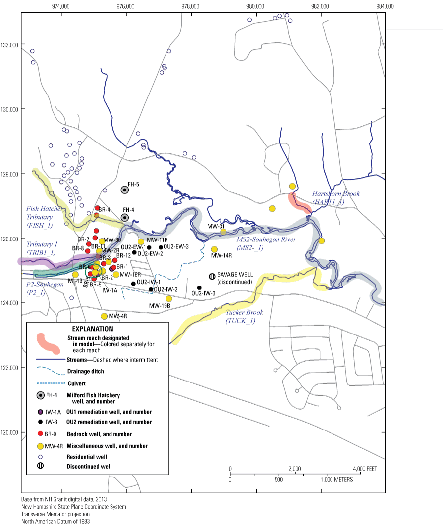
Map showing selected wells and stream segments used in the area-wide model, Savage Municipal Water-Supply Well Superfund site, Milford, New Hampshire. OU1, operable unit 1; OU2, operable unit 2.
Appendix 2. Flux Linkage Between the Area-Wide Model and the Milford-Souhegan Glacial Drift Aquifer Model, Savage Municipal Water-Supply Well Superfund Site in Milford, New Hampshire

Map showing overlay of model cells for the area-wide model and the Milford-Souhegan glacial drift aquifer model, Savage Municipal Water-Supply Well Superfund site, Milford, New Hampshire.
References Cited
Banta, E.R., Paschke, S.S., and Litke, D.W., 2008, User guide and documentation for five MODFLOW ground-water modeling utility programs: U.S. Geological Survey Techniques and Methods, book 6, chap. A28, 24 p., accessed 2012 at https://doi.org/10.3133/tm06A28.
Harte, P.T., 2004, Simulation of source transport of tetrachloroethylene in ground water of the glacial-drift aquifer at the Savage municipal water-supply well superfund site, Milford, New Hampshire, 1960–2000: U.S. Geological Survey Scientific Investigations Report 2004–5176, 78 p. [Also available at https://doi.org/10.3133/sir20045176.]
Harte, P.T., 2012, Evaluation of modeling for groundwater flow and tetrachloroethylene transport in the Milford-Souhegan glacial-drift aquifer at the Savage municipal water-supply well superfund site, Milford, New Hampshire, 2011: U.S. Geological Survey Open-File Report 2012–1079, 29 p. [Also available at https://doi.org/10.3133/ofr20121079.]
Harte, P.T., and Watt, M.K, 2021, MODFLOW–2005, MODPATH, and MOC3D used for groundwater flow simulation, pathlines analysis, and solute transport in the crystalline-rock aquifer in the vicinity of the Savage Municipal Water-Supply Well Superfund site, Milford, New Hampshire: U.S. Geological Survey data release, https://doi.org/10.5066/F7J102FK.
Winston, R.B., 2009, ModelMuse—A graphical user interface for MODFLOW–2005 and PHAST: U.S. Geological Survey Techniques and Methods, book 6, chap. A29, 52 p. [Also available at https://doi.org/10.3133/tm6A29.]
Conversion Factors
U.S. customary units to International System of Units
Datums
Vertical coordinate information, mean sea level (msl), is referenced to the National Geodetic Vertical Datum of 1929 (NGVD 29).
Horizontal coordinate information is referenced to North American Datum of 1983 (NAD 83).
Altitude, as used in this report, refers to distance above the vertical datum.
Supplemental Information
Concentrations of chemical constituents in water are given in parts per billion, which are equivalent to micrograms per liter (µg/L).
Two statistical means were used to compare the difference between observed and model-computed heads (residuals). An absolute mean was used to examine the total error inherent in the simulation, and a standard mean (called mean) was used to show the fit of the simulation. Absolute mean head difference is calculated from the summation of the absolute head difference divided by number of comparisons. A standard mean head difference indicates whether the model-computed heads are, on the average, greater than measured heads (negative difference or residual) or less than measured heads (positive difference or residual).
Random error in the simulation, even if large, could result in a standard mean that is near zero if an equal distribution of positive and negative residuals exists; however, the absolute mean difference tends to reflect random error.
Residuals are weighted to allow a meaningful comparison of measurements with different units (weighted residuals are dimensionless) and to reduce the influence of measurements with large errors or uncertainty.
Abbreviations
bls
below land surface
CSS
composite scaled sensitivities
EPA
U.S. Environmental Protection Agency
GMG
Geometric Multigrid package
kh
horizontal hydraulic conductivity
kv
vertical hydraulic conductivity
MOC3D
three-dimensional method-of-characteristics groundwater flow and transport model
MODFLOW
modular three-dimensional finite-difference groundwater flow model
MODFLOW–GWT
groundwater transport module of MODFLOW
MSGD
Milford-Souhegan glacial-drift
msl
mean sea level, equivalent to the National Geodetic Vertical Datum of 1929 (NGVD29) in this report
MT3D
three-dimensional groundwater solute transport model
NHDES
New Hampshire Department of Environmental Services
OU
operable unit
PCE
tetrachloroethylene
ppb
parts per billion
USGS
U.S. Geological Survey
For more information, contact
Director, New England Water Science Center
U.S. Geological Survey
10 Bearfoot Road
Northborough, MA 01532
dc_nweng@usgs.gov
or visit our website at
https://www.usgs.gov/centers/new-england-water
Publishing support provided by the Pembroke Publishing Service Center
Disclaimers
Any use of trade, firm, or product names is for descriptive purposes only and does not imply endorsement by the U.S. Government.
Although this information product, for the most part, is in the public domain, it also may contain copyrighted materials as noted in the text. Permission to reproduce copyrighted items must be secured from the copyright owner.
Suggested Citation
Harte, P.T., 2021, Numerical modeling of groundwater flow in the crystalline-rock aquifer in the vicinity of the Savage Municipal Water-Supply Well Superfund site, Milford, New Hampshire: U.S. Geological Survey Scientific Investigations Report 2020–5137, 47 p., https://doi.org/10.3133/sir20205137.
ISSN: 2328-0328 (online)
Study Area
| Publication type | Report |
|---|---|
| Publication Subtype | USGS Numbered Series |
| Title | Numerical modeling of groundwater flow in the crystalline-rock aquifer in the vicinity of the Savage Municipal Water-Supply Well Superfund site, Milford, New Hampshire |
| Series title | Scientific Investigations Report |
| Series number | 2020-5137 |
| DOI | 10.3133/sir20205137 |
| Publication Date | November 16, 2021 |
| Year Published | 2021 |
| Language | English |
| Publisher | U.S. Geological Survey |
| Publisher location | Reston, VA |
| Contributing office(s) | New England Water Science Center |
| Description | Report: ix, 47 p.; Data Release |
| Country | United States |
| State | New Hampshire |
| City | Milford |
| Other Geospatial | Savage Municipal Water-Supply Well Superfund Site |
| Online Only (Y/N) | Y |
| Additional Online Files (Y/N) | N |