

Groundwater Chemistry, Hydrogeologic Properties, Bioremediation Potential, and Three-Dimensional Numerical Simulation of the Sand and Gravel Aquifer at Naval Air Station Whiting Field, near Milton, Florida, 2015–20
Links
- Document: Report (4.94 MB pdf) , HTML , XML
- Dataset: USGS National Water Information System database - USGS water data for the Nation
- Data Release: USGS data release - MODFLOW simulator used to assess groundwater flow for the Whiting Field Naval Air Station, Milton, FL
- Download citation as: RIS | Dublin Core
Acknowledgments
The authors thank the following individuals for contributing to the study: Ms. Shannon Provenzano, Remedial Project Manager, Naval Facilities Engineering Systems Command Southeast; Ms. Brooke Boyd, Mr. John “Jeff” Kissler, Mr. Jonathan Stewart, Mr. Billy Ryan, and Mr. Charles Egri of the Installation Environmental Program, Naval Air Station Whiting Field; Mr. Alex Eddington, Mr. Bill Duffy, and Mr. Ryan Samuels of Resolution Consultants, Inc.; and Mr. Sam Naik, of Tetra Tech.
The authors thank Ms. Katherine “Katt” Pappas, Ms. Stephanie Phillips, Mr. Bruce G. Campbell, Dr. Francis H. Chapelle (retired), and Dr. Paul M. Bradley of the U.S. Geological Survey.
Abstract
The U.S. Geological Survey completed a study between 2015 and 2020 of groundwater contamination in the sand and gravel aquifer at a Superfund site in northwestern Florida. Groundwater-quality samples were collected from representative monitoring wells located along a groundwater-flow pathway and analyzed in the field and laboratory. In general, ambient groundwater in the sand and gravel aquifer is acidic, dilute, and oxic. Groundwater age-dating results indicate recharge to the contaminated parts of the aquifer occurred between the 1970s and 1980s. Natural gamma, electromagnetic induction, and borehole nuclear magnetic resonance logs indicated that aquifer hydraulic conductivities generally increased with depth as the aquifer formation material became coarser, characteristic of a prograding marginal-marine delta depositional environment. Aquifer formation material incubated with radiocarbon (carbon-14) cis-1,2-Dichloroethylene demonstrated biodegradation directly to carbon dioxide in contaminated and uncontaminated parts of the aquifer. A three-dimensional, numerical groundwater-flow MODFLOW model of the sand and gravel aquifer in the study area was constructed. The calibrated model reasonably reproduced measured groundwater heads and streamflows. Moreover, the model can be used to run simulations of outcomes of potential remedial strategies, such as monitored natural attenuation, as part of future feasibility studies in the area.
Introduction
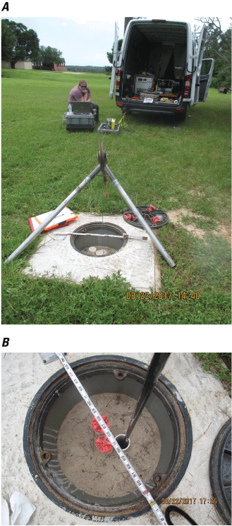
Naval Air Station Whiting Field is near Milton, Florida, (fig. 1) and has been in continuous use for airplane and helicopter flight instruction since 1943. In support of these operations, chemicals such as paint-stripping compounds, cleaning solvents, alkaline cleaners, detergents, mineral spirits, methyl ethyl ketone, isopropyl alcohol, oils, and hydraulic fluids were used. Wastes generated from the use of these chemicals were placed onsite in disposal pits, dry wells, landfills, and waste-oil bowsers, as was common practice before the formation of the U.S. Environmental Protection Agency (EPA) in 1970. Some waste disposal sites also were used in firefighting training (fig. 2A).
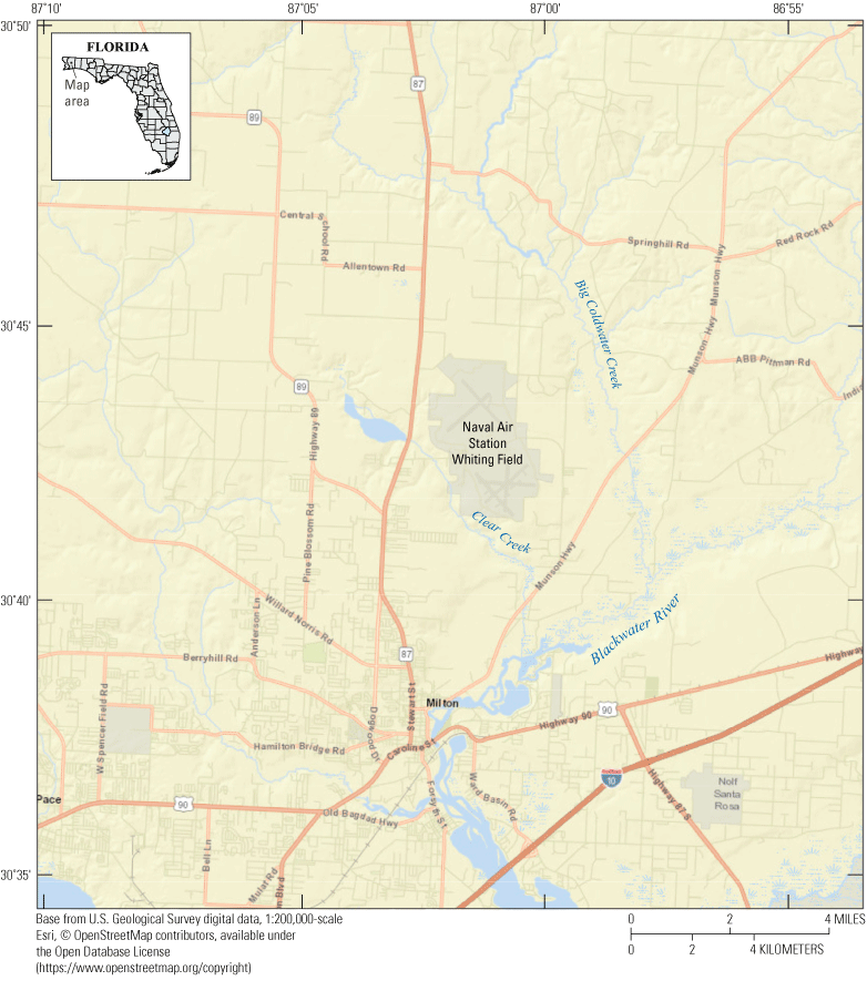
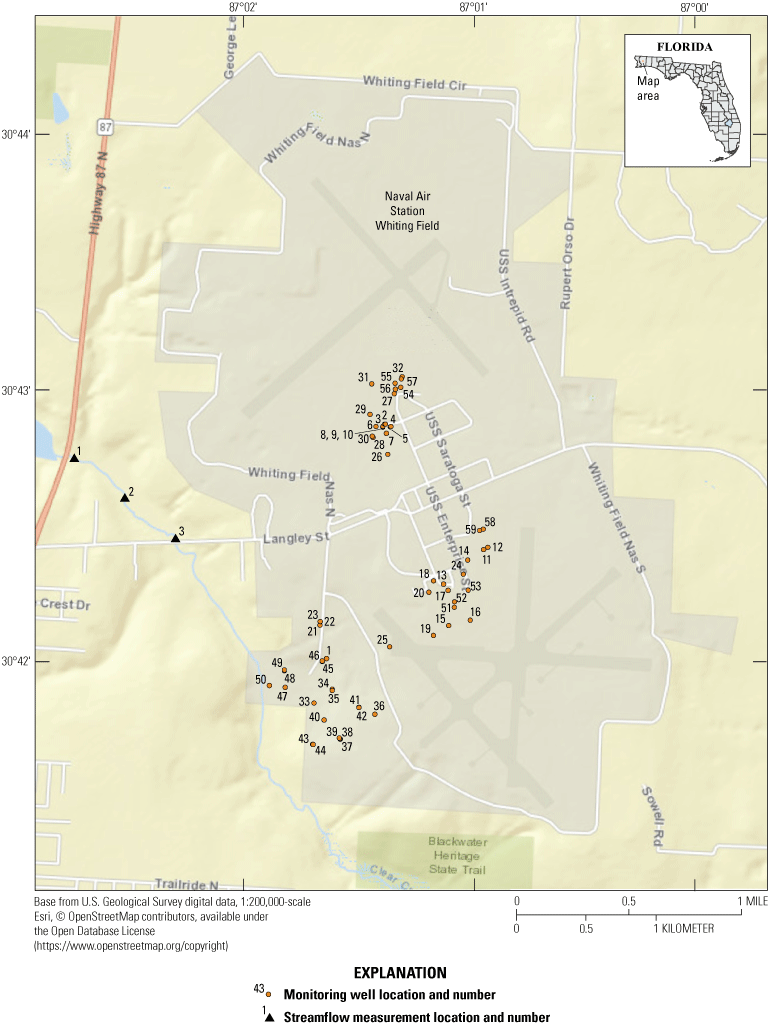
Location of Naval Air Station Whiting Field, primary surface-water features, and roads, near Milton, Florida.
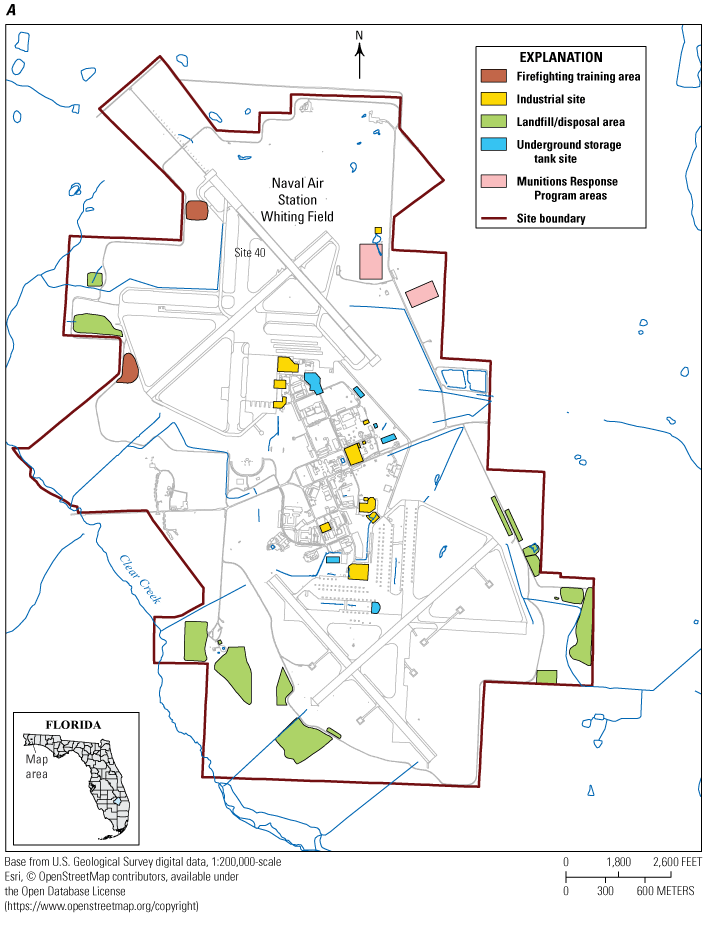
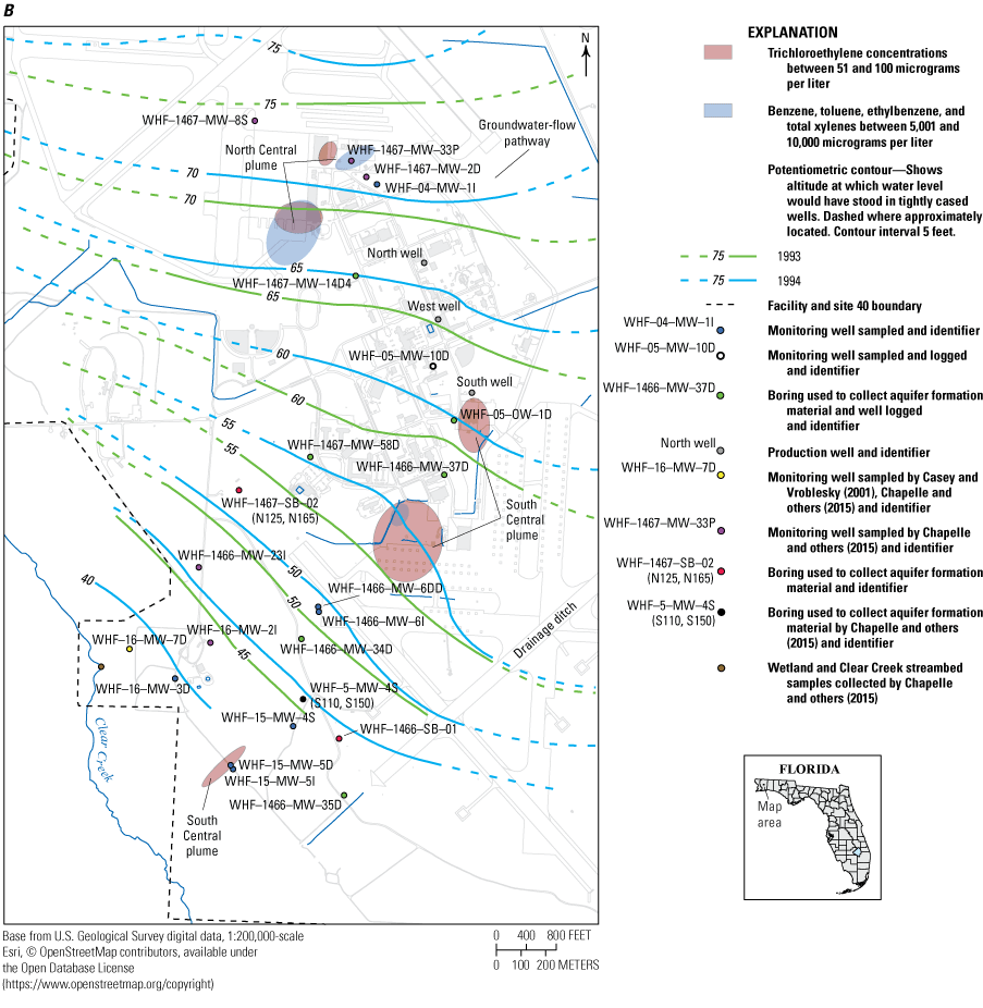
(A) Naval Air Station Whiting Field boundary and locations of known disposal areas, regulatory site identification, and firefighting training areas; (B) the potentiometric surface and generalized direction of groundwater flow in the sand and gravel aquifer and the generalized locations of the north-central and south-central plumes (modified from U.S. Navy [2012]) and locations of production wells and borings used to supply aquifer formation material for the bioremediation potential study, near Milton, Florida.
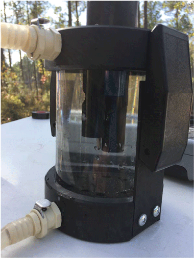
An initial site assessment at Naval Air Station Whiting Field in 1985 indicated that thousands of gallons of waste, including paints, paint thinners, solvents, waste oils, gasoline, hydraulic fluids, aviation gasoline, tank bottom sludges, and paint-stripping wastewater, may have been dumped into the onsite disposal areas (U.S. Navy, 2012). In 1985, benzene and trichloroethylene were detected in samples of drinking water collected from two of the three onsite production wells (the west well and the south well; fig. 2B) screened in the sand and gravel aquifer (Agency for Toxic Substances and Disease Registry, 2000). Additional assessments since 1986 have indicated the multiple waste disposal sites across Naval Air Station Whiting Field led to the development of contamination of the unsaturated zone beneath some sites and ultimately the development of a north-central plume and a south-central plume in the sand and gravel aquifer (see U.S. Navy [2012] and references therein; fig. 2B). The north-central plume consists of chlorinated solvents and aviation fuel and originated at land surface at disposal areas or dry wells. The south-central plume consists of chlorinated solvents and aviation fuel that also originated at land surface from similar sources (U.S. Navy, 2012). The extent of both plume boundaries and contaminant concentrations within each plume have been monitored as part of ongoing remedial investigations by the U.S. Navy Installation Restoration Program (U.S. Navy, 2012). Since 1987, groundwater pumped from all three production wells onsite has been treated by being passed through granulated activated carbon (fig. 3; U.S. Navy, 2012). Granulated activated carbon treatment technology is commonly used to remove organic contaminants from water before potable use.
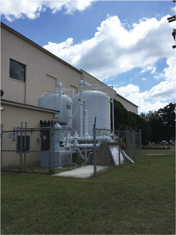
Two tanks that contain granulated activated carbon remove by adsorption contaminants from groundwater pumped from the sand and gravel aquifer by all three production wells onsite, Naval Air Station Whiting Field, near Milton, Florida. The granulated activated carbon system for the west well is shown here. [Photograph by James E. Landmeyer, U.S. Geological Survey]
Purpose and Scope
The purpose of this report is to document the results of an assessment by the U.S. Geological Survey (USGS) from 2015 to 2020 of the groundwater chemistry, hydrogeologic properties, bioremediation potential, and three-dimensional (3D) numerical simulation of groundwater flow in the sand and gravel aquifer beneath Naval Air Station Whiting Field, near Milton, Fla. The groundwater chemistry investigation included the collection in 2015 of groundwater samples from eight previously existing monitoring wells in uncontaminated parts of the aquifer. Physical properties and chemical constituents of groundwater, such as temperature, dissolved oxygen, specific conductance, and pH of the groundwater sampled, are reported along with the concentration of chlorofluorocarbons (CFCs), such as trichlorofluoromethane (CFC-11), dichlorodifluoromethane (CFC-12), and 1,1,2-Trichloro-1,2,2-trifluoroethane (CFC-113), and dissolved gases, such as methane, carbon dioxide, nitrogen, oxygen, and argon, and were used for age-dating purposes. The hydrogeologic properties investigation included collection of geophysical logs of seven monitoring wells near known contaminant source areas or the north-central and south-central plumes using natural gamma, electromagnetic induction (EMI), and borehole nuclear magnetic resonance (bNMR) tools during two events between 2017 and 2018. The bioremediation potential assessment of cis-1,2-Dichloroethylene was completed using aquifer formation material collected during installation of three monitoring wells in 2018 by the U.S. Navy. Finally, to integrate previously existing and new data, a 3D numerical groundwater-flow model of the sand and gravel aquifer and unsaturated zone was developed using the USGS modular finite-difference groundwater-flow model MODFLOW-NWT (Niswonger and others, 2011).
Previous Investigations
Multiple studies have been completed at Naval Air Station Whiting Field to investigate groundwater contamination since 1985 when contaminants were first detected in two of the three production wells that tap the sand and gravel aquifer (Agency for Toxic Substances and Disease Registry, 2000; see U.S. Navy [2012] and references therein). After Naval Air Station Whiting Field was placed on the National Priorities List in 1994, the EPA and Florida Department of Environmental Protection assigned all groundwater beneath the site boundary of Naval Air Station Whiting Field a single regulatory entity, called site 40 (U.S. Navy, 2012; fig. 2A). This was done to address the then lack of understanding of the relation between known waste disposal source areas at land surface and the north-central and south-central plumes (U.S. Navy, 2012). Field activities and analytical results of multiple soil and groundwater investigations to characterize the nature and extent of toxic and hazardous chemicals in soil and groundwater that present potential risks to human and ecological receptors were documented by the U.S. Navy (2012). The data were used by the U.S. Navy to create a conceptual site model of contaminant sources and groundwater contamination for Naval Air Station Whiting Field; a conceptual site model is required as part of the EPA Superfund process (U.S. Environmental Protection Agency, 2011) and provides a process to synthesize information regarding the physical characteristics of the site, sources of contamination, and contaminant fate and transport.
In 1998, benzene was detected in a deep monitoring well (WHF–16–MW–7D) near Clear Creek at the southwestern perimeter of Naval Air Station Whiting Field (fig. 2B; Casey and Vroblesky, 2001). Casey and Vroblesky (2001) determined the benzene originated near a former underground fuel tank area at least 1.5 miles (mi) upgradient from Clear Creek, rather than nearby former landfill/disposal areas (fig. 2A), because tritium and helium concentrations indicated the groundwater in the sampled monitoring well had been recharged around 1973.
Chapelle and others (2015) collected groundwater samples along a groundwater-flow pathway through the north-central plume. They reported that as uncontaminated, ambient groundwater from upgradient areas flowed beneath source areas, concentrations of the petroleum hydrocarbons benzene and toluene increased to about 900 and 200 micrograms per liter (µg/L), respectively (fig. 4A). Concentrations of trichloroethylene and cis-1,2-Dichloroethylene also increased. As groundwater flowed downgradient and away from the source areas, concentrations of all contaminants decreased (fig. 4A).
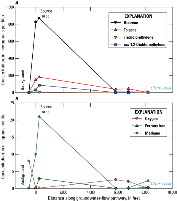
(A) Changes in contaminant concentrations along a groundwater-flow pathway as ambient groundwater flows through groundwater beneath source areas, then discharges to Clear Creek, and (B) changes in redox sensitive indicators along a groundwater-flow pathway as ambient background groundwater flows through the aquifer beneath source areas, then discharges to Clear Creek (modified from Chapelle and others, 2015).
The magnitude of contaminant concentration decreases between wells along the groundwater-flow pathway indicated that in addition to sorption and dilution processes, biodegradation processes also were responsible. Benzene and other petroleum hydrocarbons, such as toluene, and chlorinated ethenes, such as cis-1,2-Dichloroethylene and vinyl chloride, are subject to efficient biodegradation under oxic conditions whereas chlorinated ethenes, such as trichloroethylene, are subject to efficient biodegradation under methanogenic conditions (Chapelle and others, 2015). The high concentrations of dissolved oxygen associated with ambient groundwater decreased to 0 milligrams per liter (mg/L) beneath contaminated source areas and only increased to 2 mg/L in groundwater in downgradient areas near Clear Creek (fig. 4B). In contrast, concentrations of the microbially active species ferrous iron and methane were low in ambient oxic groundwater, but concentrations of both increased beneath contaminated source areas because of iron-reducing and methanogenic conditions (fig. 4B). Finally, although low concentrations of dissolved oxygen were measured in groundwater near Clear Creek, these low concentrations were related to the biodegradation of high levels of dissolved organic matter associated with the riparian zone and flood plain, rather than contamination. As a consequence, concentrations of dissolved iron and methane increased there as well (Chapelle and others, 2015).
To further examine the relation between biodegradation of contaminants and the prevailing redox conditions in groundwater in the sand and gravel aquifer at Naval Air Station Whiting Field, Chapelle and others (2015) collected aquifer formation material from the sand and gravel aquifer. The subsurface samples were collected by rotosonic coring from depths of 110 and 150 feet (ft) below land surface (bls) during the installation of a monitoring well in the south-central plume (samples S110 and S150, location on fig. 2B) and from 125 and 165 ft bls during the installation of a monitoring well (samples N125 and N165, location on fig. 2B) in the north-central plume. Additional aquifer formation material was obtained from the streambed and adjacent wetlands of Clear Creek (fig. 2B) using a hand auger. The potential for biodegradation of benzene and cis-1,2-Dichloroethylene in these samples under oxic and anoxic laboratory conditions was assessed. Oxic and anoxic laboratory microcosms were amended with uniformly labeled (UL) [UL ring-carbon-14] benzene or cis-1,2-Dichloroethylene labeled with carbon-14 at the first and second carbons ([1,2-14C] cis-DCE) and concentrations of carbon dioxide containing carbon-14, ethene containing carbon-14, and methane containing carbon-14 were monitored at 60, 121, and 238 days using gas chromatography with radiometric detection to assess biodegradation processes. Chapelle and others (2015) reported that under oxic conditions and after 238 days, [UL ring-carbon-14] benzene was transformed to nearly 100 percent of the theoretical yield for carbon dioxide containing carbon-14 in all experimental treatments for both depths at both locations (fig. 5, light blue bars for oxic and peach bars for autoclaved [dead] controls). Under anoxic conditions, [UL ring-carbon-14] benzene was transformed to between 90 and 100 percent carbon dioxide containing carbon-14 at S150 and N165 (fig. 5, dark blue bars for anoxic and dark brown bars for autoclaved [dead] controls). Under oxic conditions, [1,2-14C] cis-DCE was transformed to 35, 65, 48, and 50 percent for treatments that contained material from S110, S150, N125, and N165, respectively (fig. 5, red bars for oxic and light tan bars for autoclaved [dead] controls). Under anoxic conditions, [1,2-14C] cis-DCE indicated transformation to 35 and 15 percent carbon dioxide containing carbon-14 for the S150 and N165 aquifer formation material, respectively (fig. 5, dark red bars for anoxic and dark yellow for autoclaved [dead] controls). Moreover, no substantial accumulation of methane containing carbon-14 was observed in any treatments or carbon-14 alkenes in the anoxic treatments that contained [1,2-14C] cis-DCE.
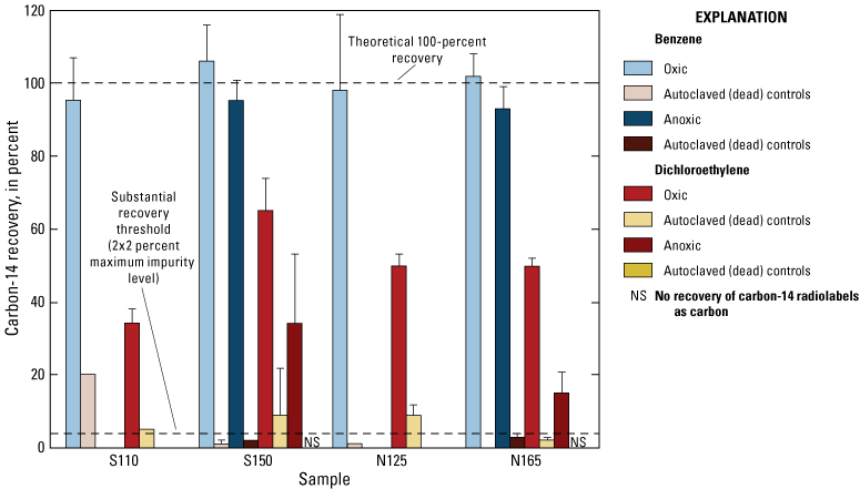
Percentage of recovery of carbon-14 radiolabel as carbon dioxide containing carbon-14 in oxic and anoxic microcosms after 238 days. For benzene, the light blue bars are for oxic and the peach bars are for autoclaved (dead) controls; the dark blue bars are for anoxic and the dark brown bars are for autoclaved (dead) controls. For dichloroethylene, the red bars are for oxic and the light tan bars are for autoclaved (dead) controls; the dark red bars are for anoxic and the dark yellow bars are for autoclaved (dead) controls. Data are averages plus or minus the standard deviation for the number of replicates. Anoxic conditions were examined for samples S150 and N165 only. No substantial accumulation of methane containing carbon-14 in any treatment or alkenes containing carbon-14 in anoxic dichloroethylene treatments was observed (modified from Chapelle and others, 2015).
These laboratory results demonstrated that a substantial part of benzene and cis-1,2-Dichloroethylene loss observed in monitoring wells along the groundwater-flow pathway in the sand and gravel aquifer (fig. 4A) was attributed to biological activity in addition to hydrodynamic processes such as dispersion or dilution. Chapelle and others (2015) also reported that microcosms that contained streambed and wetland material indicated mineralization of [UL ring-carbon-14] benzene to carbon dioxide containing carbon-14 under oxic and anoxic conditions and mineralization of [1,2-14C] cis-DCE to carbon dioxide containing carbon-14 under oxic conditions (data not plotted in fig. 4). These sediments indicated substantial reductive dichlorination of [1,2-14C] cis-DCE to carbon-14 ethene and mineralization to carbon dioxide containing carbon-14 and methane containing carbon-14; moreover, the laboratory study by Chapelle and others (2015) demonstrated the potential for [1,2-14C] cis-DCE oxidation to carbon dioxide containing carbon-14 without the production of vinyl chloride. These laboratory results provided the first evidence to explain the long-observed lack of vinyl chloride in site 40 groundwater across Naval Air Station Whiting Field. Previously, it was hypothesized that the lack of vinyl chloride was due to the lack of dichloroethylene reductive dichlorination processes, a phenomenon known as “dichloroethylene stall” (Bradley, 2003, 2012).
Description of the Study Area
Naval Air Station Whiting Field is in Santa Rosa County, in the panhandle of Florida’s northwestern coastal area, 5.5 mi north of Milton (fig. 1) and 25 mi northeast of Pensacola (not shown). Naval Air Station Whiting Field was commissioned as the Naval Auxiliary Air Station Whiting Field in July 1943 and since then has continuously functioned as a U.S. Navy aviation training facility to train U.S. Navy student aviators in the operation of propeller-driven fixed-wing aircraft and helicopters (U.S. Navy, 2012). Naval Air Station Whiting Field encompasses 3,842 acres and has two airfields (north field and south field) separated by various structures that support flight operations and staff (fig. 2A). The north field is used for fixed-wing aircraft training, and the south field is used for helicopter training.
Naval Air Station Whiting Field is located amidst agricultural land to the northwest, residential and forested areas and some agricultural land to the south and southwest, and forests to the east. Most of Naval Air Station Whiting Field is on an upland area with altitudes ranging from 150 to 190 ft above mean sea level (amsl). To the west, Naval Air Station Whiting Field is partially bounded by Clear Creek with an average altitude of about 40 ft amsl. Clear Creek, and Big Coldwater Creek to the east, are tributaries of the Blackwater River (fig. 1), which ultimately discharges to East Bay (not shown). The Florida Department of Environmental Protection classifies Clear Creek and Big Coldwater Creek as Class III waters for recreation, propagation, and management of fish and wildlife. Blackwater River is classified as Outstanding Florida Water (Florida Department of Environmental Protection, 2020). Outstanding Florida Waters are of exceptional recreational and ecological significance (Florida Department of Environmental Protection, 2020).
Climate
The study area has a climate that is generally humid and subtropical with warm summers and mild winters. The average summer temperature is 81 degrees Fahrenheit (°F), and the average winter temperature is 54 °F. At Naval Air Station Whiting Field, annual average precipitation from 1987 to 1998 was 67.58 inches (in.) with an annual high of 105.48 in. and a low of 41.76 in. of precipitation (U.S. Navy, 2012). Drought conditions existed in the southeast starting in late 1998, and between then and 2007, the average annual precipitation decreased to an average of 25.42 in. with an annual high of about 35 in. and a low of about 14 in.
Physiography
Naval Air Station Whiting Field is in the Coastal Plain physiographic province and occupies a plateau characterized by low valleys to the west and east. The western valley has an average drop in altitude of about 140 ft and is deeply incised by streams and man-made concrete lined ditches that terminate near Clear Creek. These valleys were likely created by headward erosion processes during groundwater sapping, as has been described in other high altitude, well drained coastal plain sediments (Landmeyer and Wellborn, 2013).
Geology
In general, Naval Air Station Whiting Field is underlain to depths of 250 ft bls by unnamed clastics (sands, silts, clays, and gravels) of Miocene age, the Pliocene Citronelle Formation, and undifferentiated alluvium and terrace deposits of Holocene to Pleistocene age (Marsh, 1966; fig. 6). These unconsolidated sediments record sedimentation by a prograding bayhead delta facies complex that lies unconformably over the Pensacola Clay of Miocene age that overlies differentiated and undifferentiated limestones of Early- to Middle-Miocene age that compose the Floridan aquifer system (fig. 6).
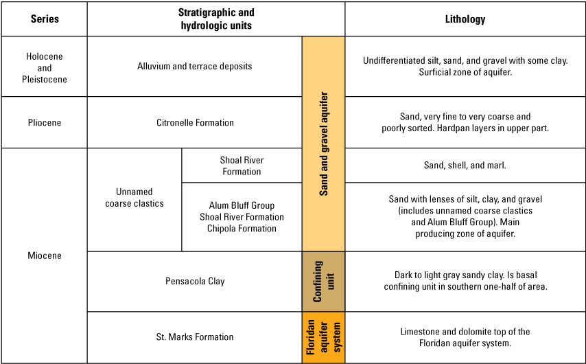
Generalized stratigraphic column, Naval Air Station Whiting Field, near Milton, Florida (modified from Marsh [1966]).
Hydrogeology
The sand and gravel aquifer at Naval Air Station Whiting Field is composed of unconsolidated Holocene and Pleistocene alluvium and terrace deposits, the Citronelle Formation, and unnamed clastics of upper Miocene age. Groundwater is present under perched to water table conditions. At the highest land-surface altitudes, depth to groundwater can be as much as 120 ft bls and represents a groundwater divide, such that recharge on the western side of Naval Air Station Whiting Field flows to the southwest to discharge to Clear Creek (fig. 2B), and conversely, recharge on the eastern side of Naval Air Station Whiting Field flows to the southeast to discharge to Big Coldwater Creek. At lower altitudes and near the creeks, springs exist where the altitude of the water table in the sand and gravel aquifer intersects the land surface. The range of horizontal hydraulic conductivities in the shallow to intermediate part of the sand and gravel aquifer that had been previously determined using rising-head and falling-head slug tests in monitoring wells was 0.34 to 49.10 feet per day (ft/d; Asea Brown Boveri Environmental Services, Inc., 1998). The range of horizontal hydraulic conductivities determined using a constant-rate, 6-day pumping test on one of the three production wells with a 7-day recovery test was 100 to 150 ft/d (Asea Brown Boveri Environmental Services, Inc., 1998). The Pensacola Clay (fig. 6) underlies the study area and was described by Hayes and Barr (1983) as a regional confining unit with low permeability.
Site 40 Groundwater
Groundwater in the sand and gravel aquifer beneath Naval Air Station Whiting Field was designated by the EPA and Florida Department of Environmental Protection in 1999 as composing a single regulatory entity called site 40 (fig. 2A), as mentioned previously. The designation of groundwater beneath Naval Air Station Whiting Field as a single site was promulgated because all presumed source areas for the north-central and south-central plumes had not been completely delineated, and known source areas were being handled as separate regulatory entities with their own unique site numbers (U.S. Navy, 2012).
Methods
Multiple methods were used between 2015 and 2020 to assess the groundwater chemistry, hydrogeologic properties, bioremediation potential, and 3D numerical simulation of the sand and gravel aquifer at Naval Air Station Whiting Field, near Milton, Fla. The locations of all groundwater and aquifer formation material samples collected, monitoring wells logged, and monitoring wells used to provide data to develop the 3D numerical model are provided on figure 2B.
Groundwater Chemistry
Groundwater samples were collected from eight previously existing monitoring wells at Naval Air Station Whiting Field (fig. 2B). The sampled monitoring wells were selected because each well (1) was located along a groundwater-flow pathway from the highest altitudes that characterize the central part of Naval Air Station Whiting Field and represented clean background conditions for groundwater to lower altitudes in downgradient areas near Clear Creek, (2) had previous groundwater sample results that indicated a lack or low level of contamination (U.S. Navy, 2012), and (3) had dissolved oxygen at a concentration high enough to support the use of CFCs to age date the groundwater along the groundwater-flow pathway.
Before groundwater sampling, previously existing location and construction data for each sampled monitoring well were used to create a unique USGS station identifier for each well. This unique information was entered into the USGS National Water Information System database (U.S. Geological Survey, 2019; table 1). The sampled monitoring wells are listed in table 1 in order of increasing relative distance along the selected groundwater-flow pathway from presumed recharge areas to Clear Creek (fig. 2B). All monitoring wells were screened across some part of the sand and gravel aquifer (table 1).
Table 1.
Monitoring well identifier, U.S. Geological Survey station identifier, total well depth, well diameter, and altitudes of top and bottom of screened interval and top of casing for monitoring wells sampled at Naval Air Station Whiting Field, near Milton, Florida.[USGS, U.S. Geological Survey; ft, foot; bls, below land surface; in., inch; amsl, above mean sea level; WHF, Naval Air Station Whiting Field site (identifier shown on fig. 2B); MW, monitoring well; I, intermediate well; D, deep well; DD, deeper well; S, shallow well]
Field Measurements
Groundwater samples were collected using a bladder pump driven by compressed air (fig. 7) and followed low-flow techniques reported in the USGS National Field Manual (U.S. Geological Survey, variously dated). At each monitoring well, the bladder pump was placed opposite the altitude of the midpoint of the screened interval. Before sample collection, groundwater was pumped through a low-flow chamber and measurements of physical properties and chemical constituents of groundwater, such as dissolved oxygen, pH, specific conductance, and temperature, were measured using a YSI 6920 sonde (YSI, Inc.). The sonde was calibrated daily before sampling using appropriate standard methods for dissolved oxygen, pH, and specific conductance as reported in the USGS National Field Manual (U.S. Geological Survey, variously dated). Groundwater samples were collected after measurements of dissolved oxygen, pH, specific conductance, and temperature had stabilized. Groundwater did not require filtration because of the low sample turbidity (fig. 8).
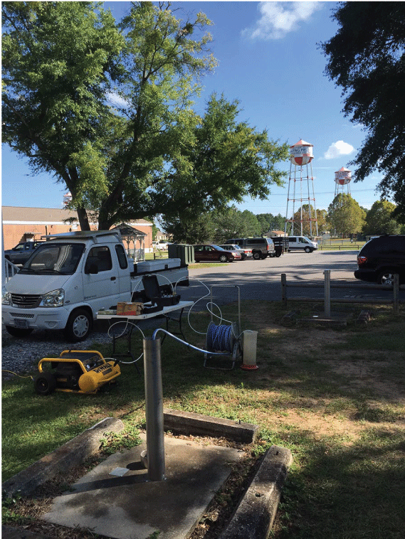
Groundwater sampling of monitoring well WHF–05–MW–10D, Naval Air Station Whiting Field, near Milton, Florida. The yellow air compressor on the left was used to drive the bladder pump that had been placed down the well and opposite the midpoint of the screened interval. The graduated nylon cylinder used for the collection of age-dating samples is shown in the center. Three of the four elevated water tanks that serve treated potable groundwater to Naval Air Station Whiting Field are shown in the background. [Photograph by James E. Landmeyer, U.S. Geological Survey]
Flow-through chamber used to measure field properties for determining when to collect a groundwater sample from the sand and gravel aquifer, Naval Air Station Whiting Field, near Milton, Florida. Note the optical clarity of the groundwater. [Photograph by James E. Landmeyer, U.S. Geological Survey]
Laboratory Analyses
Groundwater samples were collected from the monitoring wells for analyses of concentrations of CFCs and various dissolved gases. The concentrations of CFCs are necessary to age date a particular groundwater sample and, therefore, to provide important information on potential contaminant source areas, groundwater-flow pathways, and contaminant fate. In this report, the age of a groundwater sample is defined as the time elapsed since the groundwater sampled first recharged the water table (in other words, the water was removed from contact with the atmosphere) using methods described by Busenberg and Plummer (1992) and using the assumption of a piston-type flow (Plummer and Friedman, 1999). The piston-type flow model conceptualizes groundwater flow as a “plug” in a single-flow tube. Under the piston-type flow model, all groundwater-flow lines are assumed to have similar velocities, and hydrodynamic dispersion and molecular diffusion are assumed to be negligible.
The concentrations of biologically active dissolved gases, such as methane, carbon dioxide, nitrogen, and oxygen, and the inert gas argon were measured to facilitate the CFC-based age-dating process. For example, concentrations of oxygen relative to methane provided information on the redox status of groundwater and were used to interpret whether the CFC-based age dates are realistic or the CFC concentrations may have been affected by anaerobic microbial degradation. Also, the concentrations of dissolved nitrogen and argon can indicate the air temperature during past recharge events because the solubilities of nitrogen and argon vary substantially as a function of temperature (Weiss, 1970), as well as the presence of excess air entrained in groundwater during infiltration, movement through the unsaturated zone, and recharge.
Chlorofluorocarbon Concentrations
The groundwater samples for CFC analyses were collected using an approach designed to eliminate the interaction of the groundwater sample with ambient air during sample collection. Sample vials (250-milliliter [mL] glass vials) were filled beneath a volume of groundwater pumped from the monitoring well into a 2-liter graduated nylon cylinder (fig. 7). The sample tubing, made of vitex or copper to eliminate contact of the sample with air during pumping, was placed in each vial under water in the cylinder; the vial was allowed to overflow, and then each vial was capped under water using a metal screw cap with an aluminum foil liner. The samples were then removed from the cylinder, checked for the presence of air bubbles, and sealed with electrical tape around the bottle caps. The sample bottles were not stored on ice but were shipped directly to the USGS Groundwater Dating Laboratory in Reston, Virginia, where the CFC analyses were completed in triplicate using gas chromatography/mass spectrometry.
Dissolved-Gas Concentrations
The groundwater samples for dissolved-gas analyses were collected in a similar manner to those collected for the CFCs described previously, except that the dissolved-gas sample bottles were sealed with a rubber stopper. A 21-gauge needle was inserted into the rubber stopper until the tip slightly exited through the bottom of the stopper; the rubber stopper with the needle was inserted into the bottle while the bottle was submerged in the water in the 2-liter nylon cylinder, allowing any bubbles in the bottle to escape from the sample. The needle was removed from the stopper while the bottle was still submerged. Duplicate bottles were collected. All needles were properly disposed of or returned with the filled sample bottles. The sample name, water temperature, and estimated recharge altitude (the assumed altitude of the water table at the time of sampling) were recorded on the label attached to the foam sleeve used to protect the bottle during shipment. The samples were kept on ice or at least as cool as the temperature of the sampled groundwater to prevent the stoppers from popping because of sample warming. All sample bottles were stored upside down or on their side to keep any bubbles that formed away from the stopper. The sample bottles were shipped on ice to the USGS Groundwater Dating Laboratory in Reston, Va., where the dissolved-gas analyses were completed in duplicate using chromatograph/flame-ionization detection.
Hydrogeologic Properties
The USGS completed borehole geophysical logging in existing monitoring wells at Naval Air Station Whiting Field during two separate, week-long events in August 2017 and August 2018. The logging was done to further characterize the hydrogeologic properties of the unsaturated and saturated zones of the sand and gravel aquifer and to provide stratigraphic and hydrogeologic information that had not previously been collected or had been collected but at a coarser interval. Geophysical logs that were run included natural gamma, EMI, and borehole nuclear magnetic resonance logging. The theory and tools used for each borehole geophysical method are described briefly; additional theory for bNMR is provided because the data from this log were used to estimate hydraulic conductivity of the aquifer formation material as input for the 3D model.
Natural Gamma Logging
Natural gamma radiation can be used to identify changes in lithostratigraphy, which can provide an independent verification of the contact depths that are identified in drilling and lithostratigraphic logs. Borehole gamma logging measures the naturally occurring radiation of the formation material surrounding the borehole. In general, clay and fine materials emit more gamma radiation than coarser sand and gravel deposits (Keys, 1990).
Natural gamma logs were collected using a Mount Sopris Instruments natural gamma probe, model 2PGA1000. Gamma emissions were recorded, in counts per second, at depth increments of 0.1 ft. The logs were collected at 10–15 feet per minute. The vertical resolution of the gamma tool is 1–2 ft, and it can detect radiation activity through polyvinyl chloride (PVC) and steel casing materials. The contacts between coarse and fine materials are placed at the depth of one-half of the change in amplitude of the gamma response across the contact (Keys, 1990).
Electromagnetic Induction Logging
Borehole EMI logs were collected to identify changes in lithology and fluid electrical conductivity with depth. EMI logs provide a measurement of the bulk electrical conductivity of the formation and interstitial fluids surrounding the borehole (Williams and others, 1993). Changes in bulk electrical conductivity are caused by variations in porosity, in the concentrations of dissolved solids in the water, and (or) in the conductivity of the geologic matrix materials. In general, clay-rich sediments have higher conductivity than sand and gravel. The high electrical conductivity from the EMI log measurements is related to hydrostratigraphic units that contain more fine sand to clay than coarse sand and (or) highly conductive fluids such as saline groundwater, whereas low electrical conductivity in hydrostratigraphic units is related to deposits that contain coarse sand and (or) low conductivity fluids such as freshwater. When the groundwater throughout a formation consistently has low electrical conductivity, the changes in electrical conductivity within the saturated formation are mostly related to changes in lithology. EMI measurements are relatively insensitive to the electrical conductivity of the fluids in the borehole for diameters of less than 8 in. and are, therefore, effective at measuring the electrical conductivity of the geologic material and the fluids within the formation.
EMI logs were collected using a logging rate of 10–15 feet per minute with a Mount Sopris Instruments EMI probe, model 2PIA–1000. Measurements of electrical conductivity were reported in millisiemens per meter at 0.1-ft depth increments with a vertical resolution of about 2 ft. The tool is most sensitive to geologic materials about 1–1.5 ft from the tool; however, the measurement is affected to a lesser extent by materials within 5 ft of the tool in all directions (Keys, 1990). The EMI tool was calibrated with a calibration ring before logging, and the calibration was checked at the end of logging each monitoring well.
Borehole Nuclear Magnetic Resonance Logging
The bNMR logs provide measurements of water content and estimates of pore-size distribution, which can be used to estimate hydraulic conductivity of the formation surrounding the borehole. Unlike neutron logging, the bNMR method does not use active nuclear sources. In addition, bNMR is noninvasive because it does not require contact with the formation and does not require the injection or removal of fluids from the formation. The theory of the bNMR method is described in detail by Coates and others (1999), Keating and Knight (2012), and Behroozmand and others (2015). The bNMR log is based on a three-step measurement involving the spin magnetism of protons in water molecules, including (1) alignment, (2) perturbation, and (3) return to equilibrium.
In the first step, the nuclear spins of the protons in the water molecules in the formation around the borehole align to the magnetic field imposed by static magnets in the tool. The size and location of the measurement zone in the formation is a thin cylindrical shell (about 0.08 in. thick) focused at a radial distance that is targeted to be beyond the zone disturbed by drilling. For the measurement to be useful, a PVC-cased or open-hole well is required to determine hydraulic properties of the formation. In general, the radial focusing of the signal, and therefore the distance, is a function of the frequency used in the tool. In the second step, a radio-frequency pulse is generated at the Larmor frequency. The radio-frequency field is pulsed repeatedly in a specific sequence called the Carr-Purcell-Meiboom-Gill (CPMG) sequence (Carr and others, 1996). The CPMG sequence refocuses the signal strength and minimizes the effects of dephasing (signal spreading), which is caused by inhomogeneities in the magnetic field within the measurement zone. As signal strength measurements are made between the radio-frequency pulses, multiple spin-echo decays are recorded within a single CPMG scan. Typically, multiple CPMG scans are stacked to improve the signal-to-noise ratio of the measurements at a single depth. The relaxation time (Tr) is the amount of time between each repeated CPMG sequence. The full Tr must be set to a sufficiently long duration to measure the mobile water in the measurement zone. Too short of a Tr will underestimate the mobile fraction of water; however, the length of the Tr and multiple CPMG stacks increase the logging time per depth increment. Thus, a supplemental relaxation time can be set to a shorter value and stacked at a higher rate to better define the early-time decay without substantially increasing the measurement time. In the third step, between the radio-frequency pulses, the tool measures the signal strength of the decaying radio-frequency field (amplitude as a function of time) as the signal relaxes back to the background. This relaxation, or decay of the signal, is referred to as the “transverse relaxation time (T2)” or the “T2 decay.” The signal amplitude is directly proportional to water content in the measurement zone, and the timing of the T2 decay is related to the pore-size distribution; hence, the higher the amplitude, the more water is present in the measurement zone. The timing or rate of the T2 decay indicates the pore-size distribution, with fast T2 decays related to small pore sizes and long decay times related to large pore sizes. The decay time is inversely proportional to the pore size, which is a function of the surface to volume area and, hence, the interactions. In pores with greater surface areas relative to the volume of the pore, there are short T2-decay times. These two signals are fundamental in the application of bNMR to understand hydrogeologic properties of aquifers because hydraulic conductivity can be estimated using empirical relations that exploit this nuclear magnetic resonance sensitivity to water content and pore size in the saturated zone. In the unsaturated zone, the bNMR tool indicates the water content in the measurement zone.
Two bNMR tools, including the Javelin JP–175 and JP–238, manufactured by Vista Clara, Inc. (Walsh and others, 2013), were used to measure water content and estimate the pore-size distribution at Naval Air Station Whiting Field. The JP–175 bNMR tool has a diameter of 1.75 in. and fits in 2-in.-diameter wells. The JP–238 bNMR tool has a diameter of 2.38 in. and fits in 4-in.-diameter wells. Although bNMR measurements have been used in the oil industry since the 1960s, those tools are large (at least 30 ft long and 8 in. in diameter) and are heavy, requiring cable rigs to deploy the tools. In the last decade, bNMR tools have been developed for environmental applications and are lightweight, are as small as 1.75 in. in diameter, and can be easily deployed without need for a cable rig.
A few parameters are used to control the bNMR measurement by the tools. Some of the parameters are tool dependent and are specific to the tool design. The minimal echo spacing is the distance between the refocusing CPMG pulses and is tool dependent. The shorter the minimal echo spacing setting, the earlier the time decay that can be measured. The minimal echo spacing was 1.5 milliseconds for the JP–175 and 1.0 millisecond for the JP–238 for the monitoring wells logged in 2017. The minimal echo spacing was 1.0 millisecond for the JP–175, which measures earlier time decay and allows for the determination of the clay fraction, for the wells logged in 2018. In addition, two Tr values were used: a full relaxation time of 4 seconds and a burst-mode relaxation time of 0.9 second. The measurements were stacked 16 times for the full relaxation time and 96 times for the burst-mode relaxation time. The duration of the stationary measurements was about 3 minutes per measurement or about 33 feet per hour for the JP–238 and 66 feet per hour for the JP–175. The bNMR data were collected at each well logged in step mode in 3.3-ft (1.0-meter) increments for the JP–175 and in 1.6-ft (0.5-meter) increments for the JP–238, which are the vertical resolutions for each of the tools. Dual-frequency measurements were made at center frequencies of about 300 and 250 kilohertz (kHz), which relate to radial distances of about 4.0 and 5.7 in. (from the tool) in the JP–175 and JP–238, respectively.
The bNMR data were processed using the manufacturer’s software (Vista Clara, Inc., VC_Javelin_Processor, version 3.4.3). In postprocessing, the full and burst-mode (dual relaxation time) measurements were combined for each depth increment. Each frequency was processed separately, and then, frequencies were combined after processing. An impulse-noise filter was used to “despike” and remove the noisy or potentially errant data in the T2 decay. The data also were adjusted by removing the ambient noise collected with an external reference coil measured concurrently with the subsurface measurement. In addition, results from each frequency were combined, and the resultant T2 decay was fit with a multiexponential decay curve. The multiexponential decay curve was inverted to produce a pore-size distribution model for each depth using specified regularization and vertical averaging. The regularization is used to control the amount of variation and to smooth the inverted results of the pore-size distribution. Several regularization scenarios were tested to assess the best smoothing of the solution. For higher regularization values, there is more smoothing of the pore-size distribution. Multiple regularization settings, including 30, 50, 75, and 100, were tested and were assessed for variation in pore-size distribution for the simultaneous frequency-dependent measurements. This approach assumes that the zones sampled by the two frequencies, which are separated by about 1.3 centimeters, are likely similar in water content and pore-size distribution. For most of the monitoring wells logged, a regularization of 50 was selected for the final solution because it produced fairly similar results for both frequencies. A uniform regularization was used over the length of the borehole. In addition, in the interpretation program, the depth dependent measurements can be combined with adjacent depth measurements to smooth the results vertically. For these boreholes, a vertical averaging of 1 or 2 was used to smooth the results with depth.
For each depth interval, the total-, mobile-, and immobile-water fractions (as percentages) were determined using empirically derived cutoff values of T2 decay (Straley and others, 1997). The total-water content includes the mobile and immobile fractions of water. The mobile fraction, which is the fraction that decays after the 33-millisecond cutoff, represents the effective porosity. The immobile fraction, which includes the clay and capillary fractions that decay before the 33-millisecond cutoff, represents bound water. For the 2018 data, the clay-fraction cutoff was set at a relaxation time of 3 milliseconds. The output from the interpretation program included comma-separated data files for the T2 decay and the water content (including total-, mobile-, and immobile-water fractions), which were imported into the composite plots of well logs for direct comparison with the gamma, EMI, and lithostratigraphic logs.
Estimates of hydraulic conductivity were made for the fully saturated zones using bNMR data and two unit-dependent equations: the Schlumberger-Doll research (SDR) equation (Kenyon and others, 1988) and the sum of echoes (SOE) equation (Allen and others, 2000). These hydraulic conductivity values (Ksdr and Ksoe, respectively) reflect a bulk measurement. The empirical equation parameters are typically scaled to horizontal hydraulic conductivity measurements. The SDR equation uses the measured values of total porosity (ϕ) and the average log relaxation time (MLT2) as follows:
whereKsdr
is the SDR hydraulic conductivity, in meters per day;
C
is an empirically derived constant that was set to the default parameter for sand of 8,900;
m
is an empirically derived constant that is generally about 1 for unconsolidated sands (Behroozmand and others, 2015); and
n
is an empirically derived constant fixed at 2.
Ksoe
is the SOE hydraulic conductivity, in meters per day;
C
is an empirically derived constant set to 4,200; and
SE
is the measured sum of echoes.
In general, the Ksoe value is less variable with depth because the estimator is less sensitive to variations in pore size compared to the Ksdr. Conversely, the Ksdr estimator is subject to more variation based on the variation in the average log relaxation time, which varies as a function of decay time; hence, if noise is adversely affecting the decay curve or if there is early-time decay, the Ksdr will demonstrate a decrease in the estimated hydraulic conductivity for that zone that the Ksoe typically does not. The Ksdr estimates frequently indicate low hydraulic conductivity zones that are colocated with increases in natural gamma emissions, higher electrical conductivity, and clay and (or) silt in the drilling logs. These same zones may or may not be identified with the Ksoe estimates. The values used in these equations are the default parameters for sand in the processing software. As such, these estimates of hydraulic conductivity are considered order-of-magnitude estimates and are generally good relative indicators of hydraulic conductivity; moreover, estimates of Ksdr are typically more conservative than estimates of Ksoe.
The bNMR water content output from the interpretation was transferred to an Excel spreadsheet where the metric values were converted to U.S. customary units for depth and hydraulic conductivity. The Excel file was documented to record the metadata for specifics of collection and processing. The data also were imported into WellCAD for display and side-by-side comparison with the other borehole geophysical and drilling logs. A log ASCII standard (LAS) file was generated for the gamma and EMI logs. A composite plot showing all available data was generated for each borehole. All geophysical logs for all the monitoring wells logged at Naval Air Station Whiting Field are available on the GeoLog Locator online database (U.S. Geological Survey, 2020). This includes the gamma and EMI data in an LAS file, T2-decay data in an Excel file (.xlsx file), water content in an Excel file, and a composite plot of all logs in an Adobe portable document format (.pdf) file.
Monitoring Wells Logged Using Borehole Geophysical Tools
Borehole geophysical logging was completed during August 2017 at four previously existing monitoring wells (fig. 2B, table 2): WHF–05–MW–10D, WHF–1467–MW–58D, WHF–1467–MW–14D4, and WHF–05–OW–1D. Monitoring well WHF–1467–MW–58D was logged through the saturated zone in August 2017 and through the unsaturated and saturated zones in August 2018 (fig. 2B, table 2). Logs were collected in 2018 at previously existing monitoring wells WHF–1466–MW–34D, WHF–1466–MW–35D, and WHF–1466–MW–37D. At all monitoring wells logged, the gamma and EMI logs were collected first to evaluate the lithology and integrity of each monitoring well, followed by the bNMR logging of five of the seven monitoring wells. Specific information regarding each monitoring well listed in table 2 is briefly summarized in this section. The monitoring wells are listed in table 2 in order of increasing relative distance along the selected groundwater-flow pathway from presumed recharge areas to Clear Creek (fig. 2B).
Table 2.
Monitoring well identifier, U.S. Geological Survey station identifier, dates logged, and total well depth for monitoring wells logged at Naval Air Station Whiting Field, near Milton, Florida.[USGS, U.S. Geological Survey; ft, foot; bls, below land surface; WHF, Naval Air Station Whiting Field site (identifier shown on fig. 2B); MW, monitoring well; D, deep well]
For monitoring well WHF–05–MW–10D (fig. 2B), the borehole had been drilled with mud-rotary methods and split-spoon samples collected to a total depth of about 183 ft below the top of casing. For monitoring well WHF–1467–MW–14D4 (fig. 2B), an 8-in.-diameter borehole was overdrilled with mud-rotary methods to a total depth of 187 ft bls and set with a 4-in.-diameter PVC casing. Monitoring well WHF–05–OW–1D (fig. 2B) had been drilled with mud-rotary methods to a total depth of 197 ft bls. A 2-in. casing was set to a depth of 174.37 ft bls. Monitoring well WHF–1467–MW–58D (figs. 2B, 9) had been drilled with rotosonic drilling methods to a total depth of 224 ft bls with a 6-in.-diameter borehole. Three 2-in.-diameter PVC-casing wells were set within the drilled hole. Monitoring well WHF–1466–MW–34D (fig. 2B) had been drilled with rotosonic drilling methods in a 10-in.-diameter hole to a total depth of 190 ft bls. Monitoring well WHF–1466–MW–35D (fig. 2B) had been drilled with rotosonic methods to a total depth of 204 ft bls. A 2-in. casing was set to 204 ft bls. Monitoring well WHF–1466–MW–37D (fig. 2B) had been drilled with mud-rotary methods to a total depth of 200 ft bls. A 2-in. casing was set to 200 ft bls. Where available, lithologic logs prepared by a U.S. Navy contractor during the drilling of these boreholes and installation of monitoring wells are included and discussed for direct comparison to the gamma and EMI logs (Resolution Consultants, Inc., written commun., 2017).
(A) Borehole geophysical logging setup at monitoring well WHF–1467–MW–58D; (B) the deepest of the three monitoring wells shown was logged (ruler shown for scale). [Photographs by James E. Landmeyer, U.S. Geological Survey]
Bioremediation Potential
The bioremediation potential of the sand and gravel aquifer beneath Naval Air Station Whiting Field was assessed using aquifer formation material collected in 2018 by U.S. Navy contractors (Resolution Consultants, Inc.) during the drilling of boreholes for three monitoring wells. Each borehole (WHF–1466–SB–01, WHF–1467–SB–02, and WHF–1466–MW37; fig. 2B) was made using rotosonic drilling techniques that provided continuous core material free of drilling fluids and mud (table 3). The aquifer formation material was immediately removed from the rotosonic core sleeves, placed in autoclaved 1-quart mason jars, and stored on ice in coolers. The coolers were shipped to the USGS Center for Coastal & Watershed Studies, St. Petersburg, Fla., and stored in the dark in a refrigerator before the experimental setup, which is described in this section.
Table 3.
Aquifer formation material identification, depth interval of sample, and number of sample jars collected, Naval Air Station Whiting Field, near Milton, Florida.[ft, foot; WHF, Naval Air Station Whiting Field site (identifier shown on fig. 2B); SB, sediment (aquifer formation material) boring; MW, monitoring well]
Once in the laboratory, the fate of cis-1,2-Dichloroethylene under oxic and anoxic conditions was investigated following a modification of methods used by Chapelle and others (2015). The radiolabeled substrate used was [1,2-14C] cis-DCE (Moravek, Inc.), supplied at a specific activity of 7.2 millicuries per millimole and a concentration of 1.0 millicurie neat liquid, as a total volume shipped in a vial of 13.9 microliters (µL). A stock solution was prepared using 100-mL sterile Milli-Q water; all stock solutions were kept in the refrigerator to inhibit losses from the solution due to volatilization. A working solution was prepared by transferring 800 µL of the stock solution to 200 mL of sterile Milli-Q water to make a final theoretical working solution of 8.8×10⁴ decays per minute. Then, 380 µL of the working solution was added to 5.0 mL of scintillation fluid and counted on a PerkinElmer Tri-Carb 4810TR liquid scintillation counter and gave an actual working solution of 87,185 decays per minute, so the final volume dose of working solution for each sediment sample vial was 380 µL.
Two types of treatments were prepared: oxic and anoxic microcosms. Preparation of glassware included using 25-mL borosilicate glass serum vials. All vials were then washed with laboratory grade soap solution, rinsed with tap water, soaked overnight in a 10-percent (volume/volume) hydrochloric acid water bath, rinsed with tap water, and rinsed a final time in Milli-Q water. All vials were placed in an autoclavable pan, covered with aluminum foil, and sterilized. Butyl rubber plugs for serum vials were washed, rinsed, and autoclaved as described for the serum vials. The vials and plugs were moved to an operating laminar flow biological safety hood, and a sterile butyl rubber plug was aseptically (that is, wearing latex gloves that have been rinsed with ethanol) placed into each sterile vial. The vials were stored in the operating safety hood until they were filled with aquifer formation material.
To prepare the aquifer formation material slurries, Milli-Q water was first filter sterilized using a sterile membrane filter setup and membrane filters with a 0.02-micrometer pore size into a sterile borosilicate glass medium bottle. The bottle was stored in the laminar flow biological safety hood. The same procedure was used for anoxic microcosms. This volume was then autoclaved. Immediately after the autoclaving, the bottles were removed and a sterile tube was inserted and connected to a nitrogen gas source used to sparge the sterile Milli-Q water as it cooled. Sparging while the water cooled increased the rate of nitrogen gas exchange to replace the oxygen.
Killed aquifer formation material samples for the dead controls in the oxic and anoxic experiments were prepared by transferring a part of each aquifer formation material sample to separate wide-mouth jars with threaded lids and mixed to break up all the large clumps. Each killed sample of aquifer formation material went through three separate autoclaving cycles at 135 degrees Celsius (°C) at 33 pounds per square inch for 15 minutes. After each autoclaving cycle, each killed aquifer formation material sample was moved to a biological safety hood and opened, and the aquifer formation material was aggressively mixed and then placed back into the autoclave with the jar lid slightly untightened and allowed to cool until the following morning. The following day, the killed aquifer formation material was autoclaved a second time using the same parameters as on the previous day and processed afterwards as described. A third autoclaving was completed the following day, and the killed aquifer formation material was left in the autoclave to cool; the “autoclave-cooling-autoclave” cycle was done to destroy spores, mainly of the genus Bacillus. After the third autoclaving cycle and cooling to room temperature, the jar lids were tightly sealed and stored in the dark.
The nonkilled, live vials were loaded with aquifer formation material for oxic and anoxic experiments using the following approach. For oxic experiments, a 3.0-mL syringe with one end cut off was used to provide 4–5 grams of aquifer formation material per barrel. Gloves were worn and a sterile spatula scoop was used while the aquifer formation material was added into the syringe barrel. The appropriate vial was selected, and the plug was removed and placed on a tared electronic scale. The weight was recorded as that of the empty sample vial. The aquifer formation material sample syringe barrel was inserted into the sample vial using the syringe plunger to push the aquifer formation material into the vial. The total weight was recorded. The rubber plug was replaced, and the sample vial was moved off the scale. All oxic experimental vials were moved to the biological safety hood for storage during a 2-week acclimation period, covered to block all light, and stored at room temperature. For the anoxic experiments, the same steps described previously were used. Once all the vials had been loaded with the respective aquifer formation material samples, all vials were moved to the evacuation chamber of an anaerobic chamber. All rubber plugs were removed and placed into a sterile wide-mouth plastic jar. With all the open aquifer formation material sample vials in the evacuation chamber, a series of four total gas exchanges were completed before transferring the aquifer formation material sample vials and their rubber plugs into the anaerobic chamber. A gas exchange cycle exists when the existing gas in the evacuation chamber is removed via vacuum, the vacuum is turned off, then an anerobic gas mixture (5-percent hydrogen: 10-percent carbon dioxide: 85-percent nitrogen) is immediately pushed into the evacuation chamber. This cycle was repeated four times. After the fourth time of filling the evacuation chamber with the anaerobic gas mixture, the door leading into the anaerobic chamber was opened, and the aquifer formation material vials and rubber plugs were moved into that area. This method for removing the oxygen from the aquifer formation material sample vials was chosen over the standard Hungate method because of the large number of experimental vials used for this experiment. Once the vials were placed inside the main compartment of the anaerobic chamber, the rubber plugs were replaced into each of the aquifer formation material sample vials. All sealed vials were then allowed to sit in the dark at room temperature for the 2-week acclimation period.
The experimental microcosms were started after the 2 weeks of passive acclimations and while the sample vials were still in the biological safety hood. All the plugs for the oxic treatments were removed from the sample vials, and each sample vial received 2.0 mL of the sterile Milli-Q water to set up an aquifer formation material slurry in each vial. Each sample vial was dosed with 380 µL of [1,2-14C] cis-DCE working solution and immediately sealed by replacing the rubber plug. After all the sample vials had been dosed with [1,2-14C] cis-DCE and all plugs were replaced, each vial was crimp sealed and gently mixed. Dosed sample vials were then organized based on their sample site and incubation time points (the planned incubation period for the sample vials). For the anoxic treatments, after the 2-week acclimation period and while still in the anaerobic chamber, all the plugs were removed from the sample vials and 2.0 mL of sterile and anaerobic Milli-Q water (which was stored in the anaerobic chamber) was pipetted into each vial. The same procedures as outlined previously for the aerobic experiments were completed for the aquifer formation material sample vials while they were still in the anaerobic chamber.
To determine mineralization of [1,2-14C] cis-DCE to carbon dioxide containing carbon-14 after each time point, carbon dioxide containing carbon-14 was extracted from the sample vial, the decays per minute of the carbon dioxide containing carbon-14 were counted, and the results were used to determine how much of the [1,2-14C] cis-DCE was mineralized (percentage of recovery). At each time point, the sample vials from the oxic and anoxic experiments were removed from the biological safety hood or anaerobic chamber, respectively. Using a 1.0-mL hypodermic syringe and a 19-gauge needle, 1.0 mL of sulfuric acid (4N [normality]) was injected into each of the sample vials; then, the vials were gently mixed. The acid was required to lower the pH of the slurry to about 2.0, which drove the carbon dioxide containing carbon-14 in solution into the headspace. Each acidified sample vial was then stored upside down overnight to equilibrate. Collection of carbon dioxide containing carbon-14 followed, and for each acidified and equilibrated sediment sample vial, the following steps were completed. Two scintillation vials containing 5.0 mL of Carbo-Sorb E (which absorbs the carbon dioxide) were attached to the gas scrubbing system downstream from the point where the acidified sediment sample vial was attached. The vial plug of the acidified aquifer formation material sample was pierced with the needle and tubing, which were connected to the two downstream scintillation vials containing Carbo-Sorb E. The acidified sediment sample vial was pierced with a needle attached to tubing leading from a nitrogen gas source set at 60 milliliters per minute and allowed to flush the head spaces of all the vials connected to the sediment sample for 5 minutes. Each scintillation vial containing the Carbo-Sorb E was removed from the scrubbing systems, and 5.0 mL of Permafluor E+ scintillation fluid was pipetted into each vial of Carbo-Sorb E, capped, and gently mixed. The decays per minute were counted using the PerkinElmer Tri-Carb 4810TR liquid scintillation counter.
Three-Dimensional Numerical Model Development
A 3D numerical groundwater-flow model was developed to determine recharge rates, directions of groundwater flow, and discharge to creeks and streams at Naval Air Station Whiting Field. The modeling effort concentrated on developing a recharge/surface-water budget and improving the spatial distribution of aquifer properties with lithologic-log information. The model, called the Whiting Field groundwater model (WFGM), was used to examine groundwater flow relevant to contaminant source locations in Naval Air Station Whiting Field.
Groundwater-Flow Model Geometry and Discretization
The WFGM was constructed using the MODFLOW-NWT Newton Formulation for MODFLOW-2005 (Niswonger and others, 2011). Pre- and postprocessing were done with ad hoc programs, which read and write gridded data, and standard plotting programs. The WFGM was developed for an 81.06-square-mile area approximately centered on Naval Air Station Whiting Field (fig. 10). This area is 10.1 mi in the north-south direction and 8.0 mi in the east-west direction, simulated with a grid discretization of 100 ft in both horizontal directions, yielding 533 rows and 424 columns, with 9 vertical aquifer layers (fig. 11). Layer 1 extends from the top of layer 2, at an altitude of 150 ft above the North American Vertical Datum of 1988, to land surface; layers 2 through 8 are each 50 ft thick, and layer 9 is 100 ft thick. The lowest land altitude in the model area is 3.28 ft above the North American Vertical Datum of 1988; therefore, layers 1, 2, and 3 do not exist in some model areas and layer 4 can have diminished thickness (fig. 11). Other previous investigations into the sand and gravel aquifer in the Naval Air Station Whiting Field area (Asea Brown Boveri Environmental Services, Inc., 1998) indicated that, although nearby parts of the sand and gravel aquifer can be much deeper, minimal groundwater flow exists below −150 ft amsl. Based on this information, the lower two layers (layers 8 and 9) of the nine-layer WFGM were made inactive for the final simulations (fig. 11).
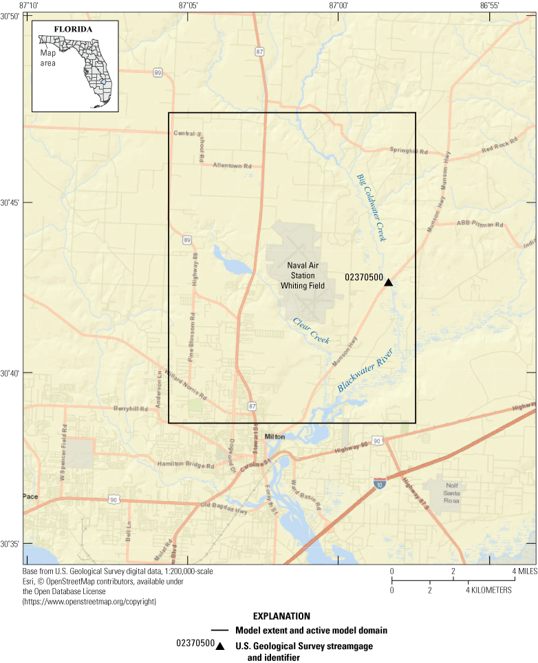
Model boundary for the Whiting Field groundwater model, Naval Air Station Whiting Field, near Milton, Florida. Also shown is the location of a long-term (since 1938) streamgage (U.S. Geological Survey station 02370500) on Big Coldwater Creek.
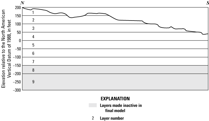
Representative north-south vertical cross section through model aquifer layers for the nine-layer Whiting Field groundwater model, Naval Air Station Whiting Field, near Milton, Florida.
Boundary Conditions and Model Stresses
The boundary conditions for the WFGM include net recharge (precipitation minus evapotranspiration) and groundwater leakage to the local creeks, such as Clear Creek and Big Coldwater Creek, and the Blackwater River (fig. 11). Groundwater flow at the lateral model boundaries is considered negligible in comparison to the other boundary conditions.
Recharge
Recharge to the sand and gravel aquifer is simulated with the MODFLOW Recharge Package (Harbaugh, 2005) in the WFGM as precipitation minus evapotranspiration. Groundwater-head measurements in the area indicate that the groundwater head is largely from 50 to 100 ft bls, far more than the defined evapotranspiration extinction depths, which nominally vary from 2 to 27 ft bls (Shah and others, 2007). Although evapotranspiration from the water table is considered negligible at the depths common in the WFGM area, some losses from interception storage and evapotranspiration in the unsaturated zone as the water percolates downward must be considered, as well as evapotranspiration from perched zones in upland areas and shallow water tables in riparian areas near creeks (fig. 10).
Groundwater Discharge to Surface-Water Bodies
The surface-water system in the WFGM is dominated by Clear Creek and Big Coldwater Creek (fig. 10). These features are represented in MODFLOW using the Drain Package (Harbaugh, 2005). The Drain Package was considered appropriate because the creeks in the area act as sinks for groundwater (fig. 10). A topographic coverage was used to generate creek locations. Control altitudes are defined by estimated average water levels in the creeks or, for dry times, the altitude of the creek bed, and the drain conductance was calibrated along with the aquifer hydraulic conductivity. As stated previously, the net recharge and the leakage to the creeks represented by the Drain Package are the external flows represented in the WFGM.
Groundwater-Head Characterization in the Study Area
Groundwater-head data were obtained from 59 previously existing monitoring wells in the study area (fig. 12, table 4). These wells were installed between 1993 and 1997 as part of the U.S. Navy’s investigation of groundwater at Naval Air Station Whiting Field. For the WFGM, 110 groundwater-head measurements made at these monitoring wells during this period were used (U.S. Navy, 2012). These wells are clustered in the central and southwestern parts of Naval Air Station Whiting Field, where the transport of contaminants toward Clear Creek is of most interest and the groundwater heads make ideal calibration targets.
Table 4.
Location number, monitoring well identifier, and average groundwater head for January–August 1997 for monitoring wells used in the Whiting Field groundwater model, Naval Air Station Whiting Field, near Milton, Florida.[ft, foot; amsl, above mean seal level; WHF, Naval Air Station Whiting Field site; MW, monitoring well; S, shallow well; D, deep well; I, intermediate well]
| Location number used in figure 12 | Monitoring well identifier | Average groundwater head (ft amsl), January–August 1997 |
|---|---|---|
| 1 | WHF–16–MW–2S | 44.34 |
| 2 | WHF–03–MW–1D | 74.73 |
| 3 | WHF–03–MW–1I | 74.87 |
| 4 | WHF–03–MW–1S | 74.92 |
| 5 | WHF–03–MW–2I | 75.07 |
| 6 | WHF–03–MW–2S | 77.19 |
| 7 | WHF–03–MW–3I | 74.58 |
| 8 | WHF–03–MW–4S | 74.87 |
| 9 | WHF–03–MW–7I | 75.17 |
| 10 | WHF–03–MW–7S | 75.18 |
| 11 | WHF–06–MW–1S | 67.3 |
| 12 | WHF–06–MW–3D | 67.72 |
| 13 | WHF–07–MW–1I | 61.83 |
| 14 | WHF–1466–MW–12S | 64.75 |
| 15 | WHF–1466–MW–15S | 59.31 |
| 16 | WHF–1466–MW–16S | 61.54 |
| 17 | WHF–1466–MW–18S | 62.76 |
| 18 | WHF–1466–MW–19S | 61.33 |
| 19 | WHF–1466–MW–1S | 57.68 |
| 20 | WHF–1466–MW–20S | 60.51 |
| 21 | WHF–1466–MW–23D | 49.3 |
| 22 | WHF–1466–MW–23I | 49.29 |
| 23 | WHF–1466–MW–23S | 49.9 |
| 24 | WHF–1466–MW–2I | 63.72 |
| 25 | WHF–1466–MW–6I | 54.63 |
| 26 | WHF–1467–MW–14S | 78.63 |
| 27 | WHF–1467–MW–20S | 78.28 |
| 28 | WHF–1467–MW–21S | 75.01 |
| 29 | WHF–1467–MW–27S | 76.34 |
| 30 | WHF–1467–MW–2I | 73.75 |
| 31 | WHF–1467–MW–31S | 78.51 |
| 32 | WHF–1467–MW–5D | 80.56 |
| 33 | WHF–15–MW–2I | 42.09 |
| 34 | WHF–15–MW–3I | 45.44 |
| 35 | WHF–15–MW–3S | 45.66 |
| 36 | WHF–15–MW–4S | 47.74 |
| 37 | WHF–15–MW–5D | 41.77 |
| 38 | WHF–15–MW–5I | 41.77 |
| 39 | WHF–15–MW–5S | 41.8 |
| 40 | WHF–15–MW–6D | 41.89 |
| 41 | WHF–15–MW–7D | 47.18 |
| 42 | WHF–15–MW–7I | 47.14 |
| 43 | WHF–15–MW–8D | 37.99 |
| 44 | WHF–15–MW–8I | 38 |
| 45 | WHF–16–MW–2D | 46.72 |
| 46 | WHF–16–MW–2I | 46.93 |
| 47 | WHF–16–MW–3I | 39.27 |
| 48 | WHF–16–MW–4D | 40.07 |
| 49 | WHF–16–MW–4II | 40.2 |
| 50 | WHF–16–MW–7D | 34.52 |
| 51 | WHF–30–MW–3S | 62.02 |
| 52 | WHF–30–MW–4S | 61.86 |
| 53 | WHF–30–MW–5S | 62.66 |
| 54 | WHF–32–MW–1S | 78.73 |
| 55 | WHF–32–MW–2S | 78.72 |
| 56 | WHF–32–MW–3S | 77.87 |
| 57 | WHF–32–MW–5S | 79.35 |
| 58 | WHF–33–MW–1S | 68.99 |
| 59 | WHF–33–MW–3S | 68.79 |
Location of monitoring wells that had previously existing groundwater-head measurements and were used for calibration of the Whiting Field groundwater model. Also shown are the locations of the streamflow discharge measurements.
Streamflow Measurements
Discrete streamflow measurements were made by the USGS at three locations along Clear Creek close to the southwestern perimeter of Naval Air Station Whiting Field (fig. 12). Each location was assigned a station number in the USGS National Water Information System database (U.S. Geological Survey, 2017). The streamflow measurements were made with a hand-held acoustic Doppler current meter (Sontek Flowtracker; Turnipseed and Sauer, 2010). These measurements were used to determine the volume of groundwater gained between upstream and downstream measurement locations for comparison with that simulated by the WFGM.
Estimating Model Hydraulic Conductivity
The model was set up with reasonable estimates of recharge, drain conductivity values, and aquifer hydraulic conductivities. The resulting initial estimated hydraulic conductivity array had the spatial variation most similar to Naval Air Station Whiting Field (fig. 13) because most of the monitoring well data were located in that area (fig. 12).
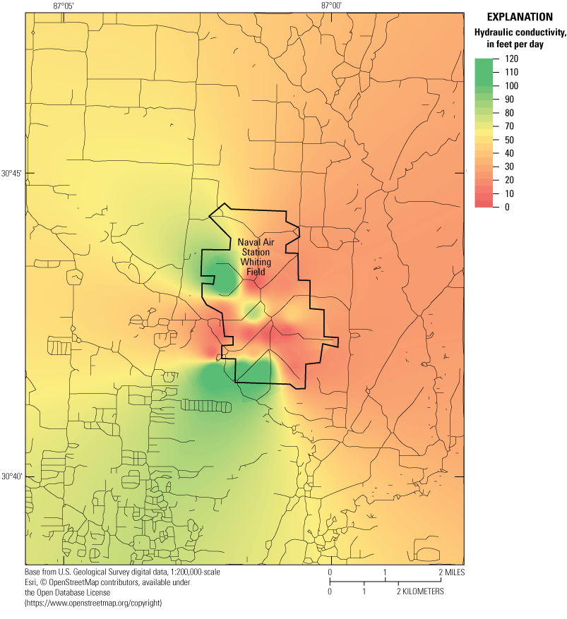
Simulated initial estimated hydraulic conductivity array in layer 1 of the Whiting Field groundwater model.
To assist in refining the model-input data, a collection of lithologic cores taken by a U.S. Navy contractor (Resolution Consultants, Inc.) provided aquifer formation-type information at various depths in numerous locations that lack monitoring wells (fig. 14), but these cores do not directly provide aquifer properties. Although standard (reference) hydraulic conductivity values for the different lithologic types exist, the hydraulic conductivities already tested in the model are certainly more relevant and specific to this study area. The lithologic type of each core was paired with the test model-input hydraulic conductivity in the corresponding model cell to combine the information in the lithologic and test model-input hydraulic conductivity arrays. The hydraulic conductivity magnitudes corresponding to each lithologic type was then used to make hydraulic conductivity adjustments. Lithologic types are listed later in the report, and details of making these adjustments are in the “Hydraulic Conductivity Values” section. Using lithologic core data to adjust hydraulic conductivity values provides a vertical variation in hydraulic conductivity.
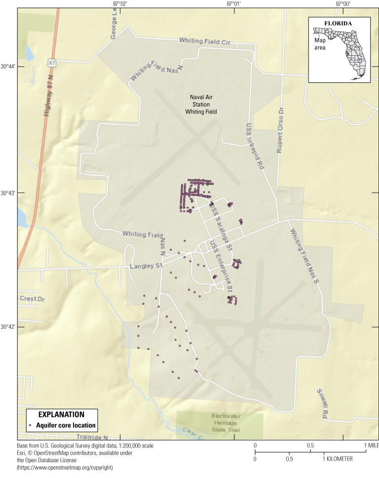
Locations of lithologic cores in the Whiting Field groundwater model area, Naval Air Station Whiting Field, near Milton, Florida.
Incorporation of the Unsaturated Zone
The unsaturated zone is directly simulated in the WFGM using the MODFLOW Unsaturated-Zone Flow Package (Niswonger and others, 2006). The Unsaturated-Zone Flow Package uses a kinematic wave approximation to Richards’ equation, solved by the method of characteristics, to simulate vertical unsaturated flow. The subsurface volume between land surface and the water table is represented with the Unsaturated-Zone Flow Package and changes with the altitude of the groundwater table. The saturated hydraulic conductivity and specific yield values that were derived for the MODFLOW-NWT flow package are used for the Unsaturated-Zone Flow Package. The relation of water content to hydraulic conductivity is defined by the Brooks-Corey equation:
where Water content is the ratio of the volume of water to the total volume of the aquifer. A standard value of ԑ=4 is used for all cells. The hydraulic conductivity values derived using this equation were compared to hydraulic conductivity values generated by the model and those calculated by the bNMR logging, as described previously.Steady-State and Transient Simulations
The average groundwater head represented for each monitoring well (table 4) was used to calibrate a steady-state version of the WFGM. The average heads were used to avoid the extreme highs and lows in groundwater heads related to storms and droughts. In the steady-state model, net recharge was calibrated by matching flow at a USGS streamgage on Big Coldwater Creek (USGS station 02370500; fig. 10; U.S. Geological Survey, 2019). The average recharge rate was used to create a quasi-steady-state transient scenario. This was followed by a daily timestep with transient precipitation for the period of June 24–July 10, 2017. This approach provided values for looking at steady-state and transient conditions and values for comparing simulated flows at creeks to measured flows at creeks and was the best use of the unsaturated-zone representation in MODFLOW-NWT.
Quality Assurance and Quality Control for Groundwater Chemistry
Data quality for the groundwater chemistry data collected was ensured using a variety of methods. All groundwater samples were collected following written protocols described in the USGS National Field Manual (U.S. Geological Survey, variously dated). Quality control samples, such as trip blanks and duplicate samples, were collected to provide information on possible sample contamination and to measure potential variability associated with the collection of data across a multiple-year study; moreover, samples were analyzed at the same laboratories to ensure consistency. Trip blanks for this study included volatile organic compound vials of laboratory blank water filled and sealed by the USGS National Water Quality Laboratory. These trip blanks accompanied environmental sample vials to verify that volatile organic compound vials were not contaminated during storage, sampling, or shipment to or from the USGS National Water Quality Laboratory. Any of the blanks described previously could have been subjected to contamination during sample collection, processing, shipping, and analysis. Duplicates were collected immediately after collection of regular environmental samples and in the same manner to provide a measure of variability because of the effects of field and laboratory procedures.
Results and Discussion of Sand and Gravel Aquifer Analysis
The results of the groundwater chemistry, hydrogeologic properties, bioremediation potential, and 3D numerical simulation of the sand and gravel aquifer at Naval Air Station Whiting Field near Milton, Fla., are described here.
Groundwater Chemistry
The results of the groundwater chemistry determined using field measurements and laboratory analyses of groundwater samples collected from the sand and gravel aquifer at Naval Air Station Whiting Field near Milton, Fla., are described in the following subsections.
Field Measurements
The results of field measurements of physical properties and chemical constituents of groundwater samples from eight monitoring wells are presented in table 5. Groundwater in the sand and gravel aquifer was characterized by the following average values of groundwater temperature (26.83 °C), specific conductance (54 microsiemens per centimeter at 25 °C [µS/cm at 25 °C]), pH (5.00), dissolved oxygen (5.06 mg/L), and dissolved oxygen percentage of saturation (63.0 percent; table 5).
Table 5.
Field measurements of physical properties and chemical constituents during groundwater sample collection at monitoring wells, Naval Air Station Whiting Field, near Milton, Florida, 2015.[USGS, U.S. Geological Survey; °C, degree Celsius; µS/cm, microsiemens per centimeter at 25 degrees Celsius; mg/L, milligram per liter; WHF, Naval Air Station Whiting Field site (identifier shown on fig. 2B); MW, monitoring well; I, intermediate well; D, deep well; DD, deeper well; S, shallow well; average values for each measurement are shown in bold at bottom of column]
The field measurements of groundwater in uncontaminated parts of the sand and gravel aquifer are, in general, similar to those of local precipitation. Most monitoring wells have groundwater that is dilute, oxygenated, and acidic, like precipitation. Groundwater samples from some wells, however, have elevated specific conductance values that indicate the interaction of groundwater with minerals in the aquifer formation material or activities at land surface. The presence of aerobic conditions in these uncontaminated or less contaminated wells supports the use of CFCs to age date the groundwater recharge, which is described next. This scenario is not representative of the anoxic redox conditions elucidated by Chapelle and others (2015), described in previous sections, because such conditions arise only if contamination by aromatic petroleum hydrocarbons or chlorinated compounds or natural organic-rich wetlands are present. The average low pH may be the result of ambient, naturally acidic precipitation caused by the dissolution of atmospheric carbon dioxide during precipitation and the fact that the sediments in the subsurface have been highly weathered. As such, there is little buffering capacity in the subsurface because the dissolution minerals such as feldspars (that would tend to increase the pH of water) have already been extensively weathered.
Chlorofluorocarbon Concentrations and Groundwater-Age Dates
The concentrations of CFC-12 and CFC-113 in all groundwater samples (table 6) are greater than what would be expected if the precipitation were in equilibrium with uncontaminated air (that is, groundwater concentrations were supersaturated relative to globally measured air-phase concentrations). These elevated concentrations may indicate that local, nonatmospheric point sources (perhaps sewage effluent or other contamination such as landfill leachate affected by leakage from buried spray cans, shredded insulation foam, or CFC-113-based solvents or as neat dense nonaqueous phase liquid released at land surface [Im and others, 2019]) have added water that contained elevated CFC-12 and CFC-113 concentrations. For example, the concentrations of CFC-113 measured in monitoring wells WHF–15–MW–5D and WHF–15–MW–4S are as much as 30 times greater than the average CFC-113 concentration of 362,815 picograms per kilogram measured in other samples, and these monitoring wells are near landfill/disposal areas in downgradient areas of Naval Air Station Whiting Field (fig. 2A). Groundwater is more likely to be contaminated by CFC-113 than either CFC-11 or CFC-12 because the former is a liquid at ordinary temperatures and can readily enter groundwater, whereas the latter two are volatile gases at ordinary temperatures. Several cases of contamination of groundwater by CFC-113 have been documented (Lesage and others, 1990; Jackson and others, 1992; Hȍhener and others, 2002).
Table 6.
Well identifier, U.S. Geological Survey station identifier, sample date and time, concentration in solution of chlorofluorocarbons in groundwater samples, piston-type flow recharge dates, and estimated recharge year from trichlorofluoromethane, sand and gravel aquifer, Naval Air Station Whiting Field, near Milton, Florida, 2015.[Triplicate samples were analyzed for concentrations of chlorofluorocarbons (CFCs), and results are reported for one sample used for dating; USGS, U.S. Geological Survey; pg/kg, picogram per kilogram; CFC-11, trichlorofluoromethane; CFC-12, dichlorodifluoromethane; CFC-113, 1,1,2-Trichloro-1,2,2-trifluoroethane; WHF, Naval Air Station Whiting Field site (identifier shown on fig. 2B); MW, monitoring well; I, intermediate well; contam., CFC concentrations are in excess of air-water equilibrium and can indicate that nonatmospheric sources (perhaps sewage effluent) have added CFCs to groundwater; D, deep well; DD, deeper well; S, shallow well]
The concentrations of CFC-11 in some groundwater samples were not greater than what would be expected if the precipitation were in equilibrium with uncontaminated air. These concentrations provided piston-type flow recharge dates from 1976 to 1980; the oldest ages in groundwater are from wells near Clear Creek. This age distribution is in rough agreement with the recharge date of around 1973 determined using tritium and helium concentrations in deep monitoring well WHF–16–MW–7D near Clear Creek (Casey and Vroblesky, 2001).
Dissolved Gases
Concentrations of methane, carbon dioxide, nitrogen, oxygen, and argon in groundwater samples collected from the monitoring wells and duplicate samples are listed in table 7. The presence of dissolved oxygen and absence of dissolved methane confirm the oxic characterization of the sand and gravel aquifer in areas not affected by contamination. The absence of methane in this background groundwater supports the use of CFC-11 for age dating because any changes in CFC-11 concentration since recharge would not be due to biodegradation. Monitoring wells WHF–15–MW–5I, WHF–1466–MW–6DD, and WHF–04–MW–11 each had a trace of detectable methane in one of the two duplicate samples (data not shown), and monitoring wells WHF–1466–MW–6DD and WHF–04–MW–1I had the highest concentrations of carbon dioxide. Nitrogen concentrations were highest in the monitoring wells that had higher concentrations of CFC-113.
Table 7.
Concentrations of methane, carbon dioxide, nitrogen, oxygen, and argon in groundwater samples, Naval Air Station Whiting Field, near Milton, Florida, 2015.[USGS, U.S. Geological Survey; °C, degree Celsius; mg/L, milligram per liter; WHF, Naval Air Station Whiting Field site (identifier shown on fig. 2B); MW, monitoring well; I, intermediate well; D, deep well; DD, deeper well; S, shallow well]
Groundwater from most monitoring wells had excess air (greater than 0.50 mg/L of argon and between 1 and 6 cubic centimeters per kilogram of excess air; fig. 15). This means that higher concentrations of argon and nitrogen were in groundwater than expected from water in equilibrium with air represented as the water in equilibrium with air line in figure 15. The excess air in these groundwater samples may reflect the entrapment of subsurface air in recharge as water moves through more than 100 ft of the unsaturated zone before entering the water table (Heaton and Vogel, 1981). Air entrapment in groundwater also may be due to fluctuations in the water table (Aeschbach-Hertig and others, 2008). It is unlikely that excess nitrogen can be explained by biological processes because denitrification is inhibited at the levels of dissolved oxygen measured in the monitoring wells.
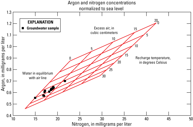
Plot of argon and nitrogen concentrations in groundwater above the water in equilibrium with air line showing the presence of excess air in groundwater attributed to recharge through the thick unsaturated zone, Naval Air Station Whiting Field, near Milton, Florida.
Hydrogeologic Properties
Lithostratigraphic descriptions from drilling logs and aquifer formation material provided by a U.S. Navy contractor (Resolution Consultants, Inc.) and results of natural gamma, EMI, and bNMR logs for each monitoring well are described in this section. All geophysical logs are electronically available at the USGS GeoLog Locator log-archive database (U.S. Geological Survey, 2020).
Geophysical Logging in 2017
Logs for monitoring wells WHF–05–MW–10D, WHF–1467–MW–58D, WHF–1467–MW–14D4, and WHF–05–OW–1D are shown and described in this section. Monitoring well WHF–1467–MW–58D was logged through the saturated zone in 2017 and through the unsaturated and saturated zones in 2018, and these combined logs are shown in the section that documents logging done in 2018.
Monitoring Well WHF–05–MW–10D
The groundwater head on August 21, 2017, was 119.10 ft below the top of casing (data not shown; fig. 16). From depths of 115–136 ft and 154–160.5 ft, there are increases in the EMI conductivity and the natural gamma counts consistent with the presence of fine-grained materials such as clay; the lithologic logs indicate the presence of clay at both depths. At the same depth intervals, the bNMR data (T2 decay, water content [total], water content [immobile], and noise) indicates a high immobile-water content fraction but low mobile-water content fraction, and the estimated hydraulic conductivity (Ksdr) ranges from 5 to 90 ft/d (table 8). The T2-decay plot shows high-intensity (hotter) colors where there is higher water content fraction. The bNMR data indicate an increase in the total-water content at a depth of about 114 ft. This zone is characterized by high gamma and EMI conductivity and is dominated with early-time decay (immobile water) consistent with clays and fine sediments. The fraction of mobile water increases at the bottom of the high gamma zone. As expected, the water content fraction declined above the water level and the clay layer, and the bNMR log was dominated by immobile water. Above the saturated zone, the bNMR response was adversely affected by electrical noise.
Table 8.
Summary of estimated hydraulic conductivity from borehole nuclear magnetic resonance data, 2017 and 2018, Naval Air Station Whiting Field, near Milton, Florida.[USGS, U.S. Geological Survey; ft, foot; bls, below land surface; Ksdr, hydraulic conductivity estimated using the Schlumberger-Doll research equation; ft/d, foot per day; Ksoe, hydraulic conductivity estimated using the sum of echoes equation; WHF, Naval Air Station Whiting Field site (identifier shown on fig. 2B); MW, monitoring well; D, deep well; NA, not applicable, no borehole nuclear magnetic resonance data collected]
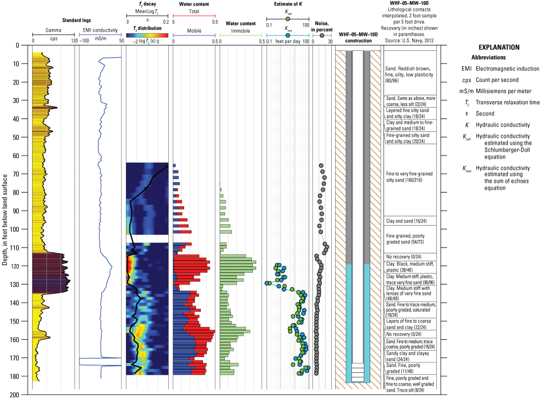
Combined geophysical logs, stratigraphic log, and well construction for monitoring well WHF–05–MW–10D, Naval Air Station Whiting Field, near Milton, Florida.
Monitoring Well WHF–1467–MW–14D4
The groundwater head was 96.47 ft bls on August 23, 2017 (data not shown; fig. 17). Over the upper part of the well, the gamma and EMI indicated variations in gamma activity and EMI conductivity, indicating changes in the lithology with depth (that is, low gamma counts and low electrical conductivity for sand units, high gamma counts and high electrical conductivity for clays). For the depth intervals of 147–209 ft, 211–255 ft, and 282–313 ft, the estimated hydraulic conductivity (Ksdr) ranged from 0.2 to 5.0 ft/d, 0.2 to 10 ft/d, and 10 to 20 ft/d, respectively (table 8). In the upper part of the well and the screened interval, it seems that much of the bNMR log is adversely affected by the original borehole construction and remnants of drilling mud. The locations where the EMI log demonstrates negative EMI conductivity values (data not shown) and the bNMR was adversely affected by the presence of steel are characterized by decreases in the measurements of the coil resonance (Q-values, dimensionless), measured water content, and estimated hydraulic conductivity values. Q-values collected as part of the bNMR log were plotted for each frequency and were used qualitatively to identify the presence of iron metal in or near the measurement zone. The drop in Q-values (and electrical conductivity values) was interpreted as the presence of centralizers behind the casing. The anomalies were observed at regular intervals at about 20–40-ft spacings. At these depths, the associated decreases in hydraulic conductivity are artifacts of the steel and are not real changes in hydraulic properties. When the borehole tools were removed from the well, they were covered with drilling mud, indicating the drilling mud is in the bottom of the well and might be in the screened interval.
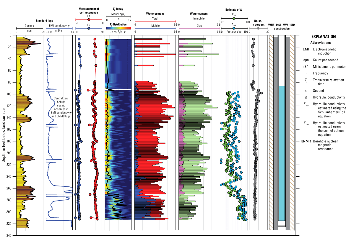
Combined geophysical logs and well construction for monitoring well WHF–1467–MW–14D4, Naval Air Station Whiting Field, near Milton, Florida.
Monitoring Well WHF–05–OW–1D
The groundwater head was measured at 121.85 ft bls (fig. 18). The natural gamma log was characterized by low gamma counts, consistent with sand, from 7 to 115 ft bls. From a depth of 115–161 ft bls, the gamma log indicates high counts consistent with either clay and fines or bentonite in the annular space. From a depth of 164 ft to the bottom of the borehole, the gamma counts are low, consistent with sand and little to no fines. The presence of the metal casing adversely affected the electrical conductivity logs and prevented the use of bNMR.
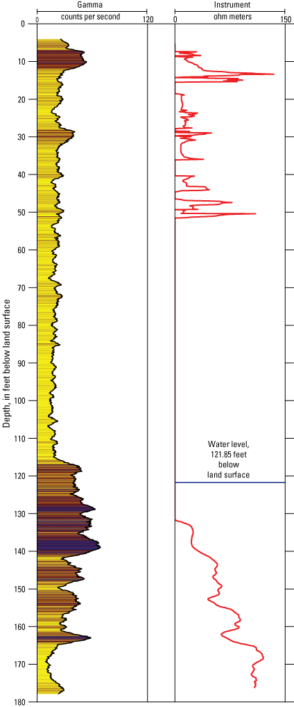
Combined geophysical logs for monitoring well WHF–05–OW–1D, Naval Air Station Whiting Field, near Milton, Florida.
Geophysical Logging in 2018
Geophysical logs are shown for monitoring wells WHF–1467–MW–58D, WHF–1466–MW–37D, WHF–1466–MW–34D, and WHF–1466–35–D in this section. As stated previously, monitoring well WHF–1467–MW–58D was logged through the saturated zone only in 2017 and through the unsaturated and saturated zones in 2018; as such, the combined results for monitoring well WHF–1467–MW–58D are shown as a single combined log in this section.
Monitoring Well WHF–1467–MW–58D
The groundwater head measured in the deepest monitoring well was 136.42 ft bls on August 22, 2017 (data not shown), and 137.97 ft bls on August 29, 2018 (data not shown; fig. 19). In the unsaturated zone from land surface to 137 ft bls, the gamma and EMI logs indicate the presence of clay and fines at depths of 8–20 ft bls and 124–132 ft bls. These two zones are characterized by immobile water and indicate only a minor fraction of mobile water (less than 0.05; 5 percent). The zone from 8 to 20 ft bls has a high total-water content fraction at about 0.4 (40 percent), with as much as 0.2 (20 percent) specified as clay content; this zone is interpreted to be bentonite related to drilling mud or well screen seal rather than a depositional unit. The estimated Ksdr for the depth interval of 149–168 ft bls and screened by the shallow monitoring well ranged from 5 to 800 ft/d (table 8). The estimated Ksdr for the depth interval of 170–188 ft bls and screened by the intermediate monitoring well ranged from 9 to 500 ft/d (table 8). The estimated Ksdr for the depth interval of 209–219 ft bls and screened by the deep monitoring well ranged from 20 to 900 ft/d (table 8). The gamma and EMI logs indicate the presence of clay and fines at depths of 153–167 ft bls, 193–197 ft bls, and 209–211 ft bls and indicate the monitoring wells are hydraulically isolated from one another even though they were installed in the same borehole.
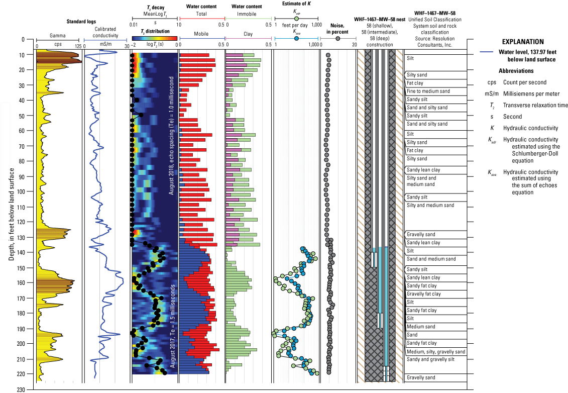
Combined geophysical logs, stratigraphic log, and well construction for monitoring well WHF–1467–MW–58D, Naval Air Station Whiting Field, near Milton, Florida.
Monitoring Well WHF–1466–MW–37D
The groundwater head was measured at 131.46 ft bls (fig. 20). High-count natural gamma zones were identified at depths of 4–11 ft bls, 23–29 ft bls, 118–134 ft bls, and 181–186 ft bls. These zones seem to coincide with clay layers in the lithology log. The EMI log indicates minor variations over the length of the well. A zone of low electrical conductivity extends from a depth of 93–106 ft bls, just above the depth to water in the well, which would be indicative of sand, but the lithology log indicates silt and silty sand. A low gamma and low electrical conductivity zone extends from 138 to 165 ft bls, which seems to coincide with the sand and silt zone. From a depth of 125–138 ft bls, the EMI conductivity indicates a small increase at the same depth as a clay layer identified in the stratigraphic log. This zone may serve as the confining unit between the deep and intermediate piezometers. A bNMR log could not be safely collected because of heavy rain and an approaching lightning storm.
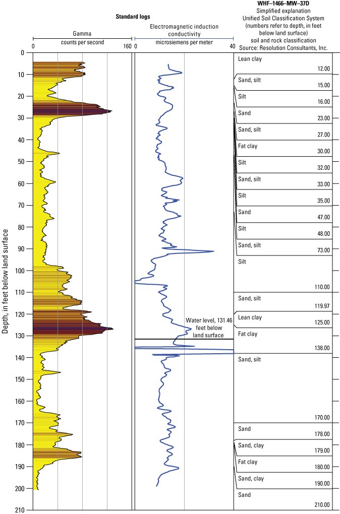
Combined geophysical logs, stratigraphic log, and well construction for monitoring well WHF–1466–MW–37D, Naval Air Station Whiting Field, near Milton, Florida.
Monitoring Well WHF–1466–MW–34D
The groundwater head on August 3, 2018, was 97.11 ft bls (fig. 21). The natural gamma log indicates a high count from 0 to 30 ft bls. Minor gamma spikes that weakly correlate to short T2 decays are seen as slightly higher amplitude in early-time decay. From 124 to 126 ft bls, 136 to 138 ft bls, and 162 to 168 ft bls, there are high gamma counts and high electrical conductivity, and these zones coincide with slightly increased clay content. From 0 to 46 ft bls, the bNMR indicates a total water content fraction of 0.5 (50 percent) that is mostly immobile water and may indicate bentonite or grout. From 46 to 97 ft bls, the unsaturated zone consists of varying amounts of water content fraction (from less than 0.10 [10 percent] to 0.25 [25 percent]) with immobile and mobile water dominated by water in the capillary and clay fraction. In the bottom of the monitoring well, in the screened interval, there is minimal to no gamma activity, coinciding with sand. The estimated Ksdr ranged from 0.5 to 8 ft/d in the interval of 100–160 ft bls, and from 0.2 to 90 ft/d in the interval of 161–180 ft bls (table 8).
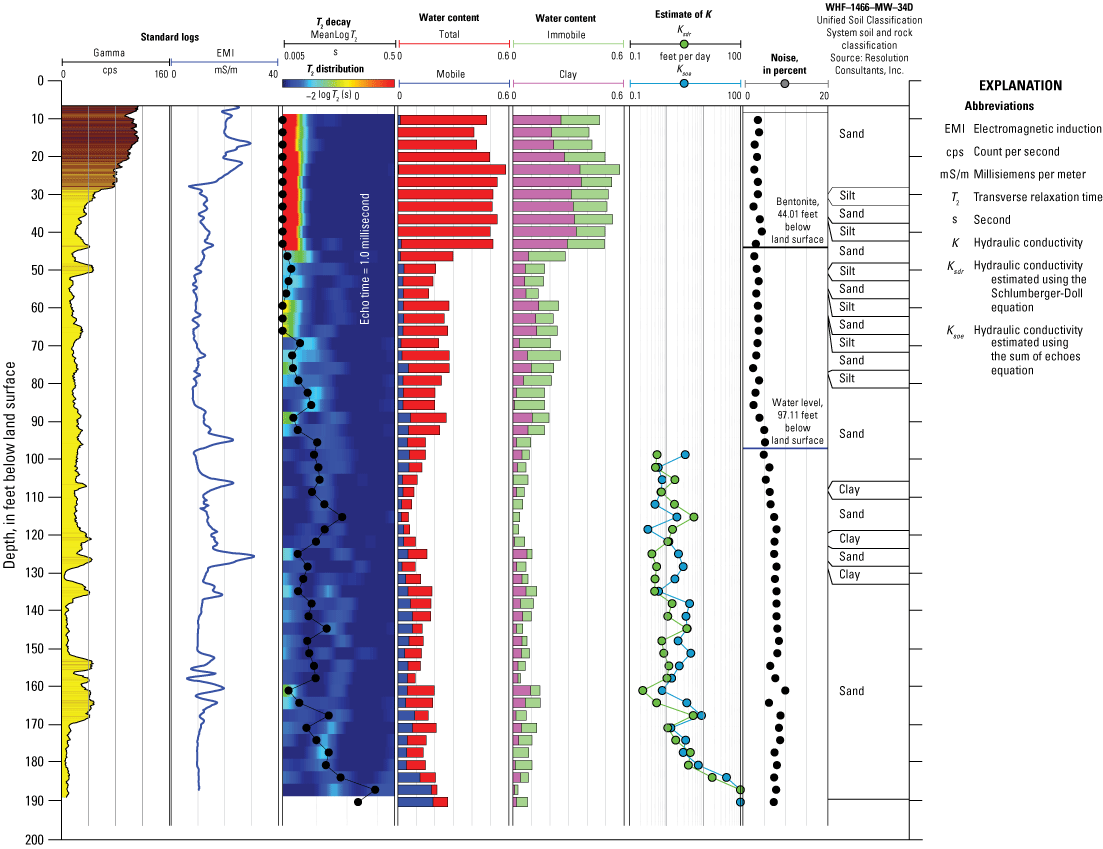
Combined geophysical logs and stratigraphic log for monitoring well WHF–1466–MW–34D, Naval Air Station Whiting Field, near Milton, Florida.
Monitoring Well WHF–1466–MW–35D
The groundwater head on August 29, 2018, was measured at 111.1 ft bls (data not shown; fig. 22). Variations in the gamma log indicate locations of increased counts that are weakly correlated to lithology dominated by clays, centered at about 61, 150, and 204 ft bls, but similar increases in gamma at depths of 4–8 ft bls, 44–49.7 ft bls, 100.4–104 ft bls, and 184–190 ft bls were associated with sand with few silts in the lithology. The EMI log could not be run past 114.83 ft bls, perhaps inhibited by a slight bend in the casing. The bNMR log measured that total water from the top of the well to a depth of 50 ft bls was immobile and, therefore, may indicate the presence of bentonite, drilling mud, or ambient conditions in the unsaturated zone. From 50 to 198 ft bls, the log was predominantly immobile water, which was not strongly correlated with natural gamma activity and may indicate some mud invasion or the presence of bentonite. The bNMR data from the screened interval at the bottom of the well indicated mobile water fraction (0.22; 22 percent). The estimated Ksdr ranged from 0.05 to 1 ft/d and 0.05 to 2 ft/d, respectively, for the depth intervals of 115–135 ft bls and 155–200 ft bls (table 8).
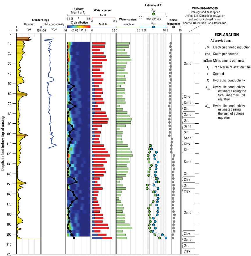
Combined geophysical logs and stratigraphic log for monitoring well WHF–1466–MW–35D, Naval Air Station Whiting Field, near Milton, Florida.
The geophysical logs collected during 2017 and 2018 indicate that the aquifer formation material underlying Naval Air Station Whiting Field consists of interbedded sands, silts, and clays. The deepest sediments are coarser, and the sediments become finer grained as they approach land surface. This change in facies is consistent with a sedimentary depositional environment commensurate with a prograding upper delta in a near shore, marginal marine paleoenvironment. Interbedded lenses of finer grained silts and clay at different depths at the same location record the shift from coarser grained sediments deposited in channels and finer grained sediments deposited over flooded banks.
Bioremediation Potential
The percentage of recovery of [1,2-14C] cis-DCE as carbon dioxide containing carbon-14 under oxic and anoxic conditions in laboratory microcosms after 329 days of incubation is shown in figure 23. The percentages of recovery in live microcosms were normalized by the percentage of recovery of the dead controls measured on day 10 because subsequent timepoints of 81 and 329 days revealed microbial activity in the dead controls, most likely attributable to the lack of additional autoclaving treatments for the dead controls over time. Under oxic and anoxic microcosm conditions, the aquifer formation material produced on average 20 and 28 percent carbon dioxide containing carbon-14 from the added [1,2-14C] cis-DCE, respectively. These values are the same order of magnitude but slightly lower than those reported by Chapelle and others (2015). The slightly lower values may reflect (1) the bacteria were using the dichloroethylene for energy and not growth; (2) the aquifer formation material collected was from parts of the sand and gravel aquifer not exposed to chronic trichloroethylene or dichloroethylene contamination, unlike the aquifer formation material used by Chapelle and others (2015) that was contaminated by trichloroethylene and dichloroethylene; (3) the dosed level of dichloroethylene in the aquifer formation material slurry microcosms may have been lower than anticipated because of volatilization of [1,2-14C] cis-DCE during addition to the microcosms; or (4) a combination of explanations. Regardless, the observed production of carbon dioxide containing carbon-14 from [1,2-14C] cis-DCE in aquifer formation material not yet exposed to dichloroethylene contamination reflects that the antecedent potential for dichloroethylene degradation exists in uncontaminated parts of the sand and gravel aquifer. These laboratory results explain the lack of observed vinyl chloride in site 40 groundwater at Naval Air Station Whiting Field is not related to the commonly known “dichloroethylene stall” phenomenon; rather, dichloroethylene is mineralized directly to carbon dioxide.
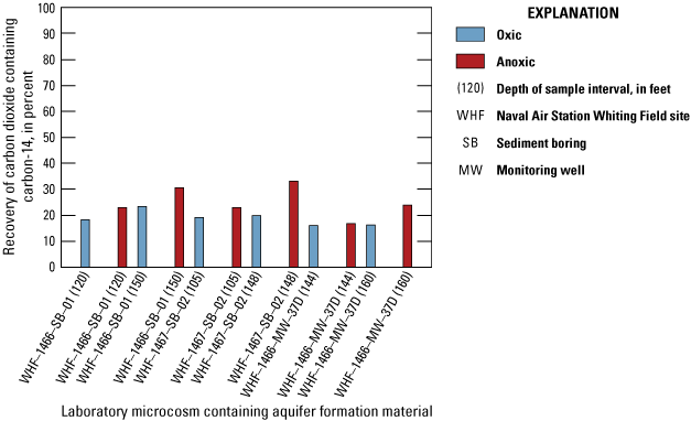
Mineralization of cis-1,2-Dichloroethylene labeled with carbon-14 at the first and second carbons ([1,2-14C] cis-DCE) to carbon dioxide containing carbon-14 in laboratory microcosms that contained aquifer formation material (table 3) from the sand and gravel aquifer under oxic (blue) and anoxic (red) conditions, after 329 days of incubation, Naval Air Station Whiting Field, near Milton, Florida.
Three-Dimensional Numerical Groundwater-Flow Model
The WFGM of the sand and gravel aquifer was developed, and the model was applied to gain insight into groundwater heads and flows around Naval Air Station Whiting Field. Simulated groundwater heads are compared with historical field measurements, and exchanges with surface-water and groundwater-flow directions are examined. All model files are electronically available at the USGS model archive database (Swain, 2021).
Hydraulic Conductivity Values
The preliminary hydraulic conductivity array was determined from general aquifer characteristics and model test simulations, as was discussed in the “Methods” section (fig. 13). Lithologic information supplied by cores of the sand and gravel aquifer improved the preliminary hydraulic conductivity array by allowing for site specific adjustments to the horizontal hydraulic conductivities. For each lithologic type identified, the model cell locations containing a log of this type are identified, and the minimum, maximum, and median of the preliminary hydraulic conductivities at these cells were calculated (table 9); therefore, statistics of the hydraulic conductivities are associated with each field-measured lithologic type. This comparison produced reasonable results; the highest median hydraulic conductivities are in silt and well-graded silty sand, whereas the lowest median hydraulic conductivities are in clayey sand and well-graded clayey sand (table 9).
Table 9.
Hydraulic conductivity statistics at locations of lithologic cores, Naval Air Station Whiting Field, near Milton, Florida.[ft/d, foot per day]
The range of hydraulic conductivities determined by this method was quite large for each lithologic type, and application to the model was not supported. Each lithologic type has a median of the horizontal hydraulic conductivities, which indicates the central tendency of the hydraulic conductivities associated with the lithologic type. Each median of horizontal hydraulic conductivity is divided by the average of all the median values of horizontal hydraulic conductivity to obtain a weighting factor that indicates the tendency of a given lithologic type to have horizontal hydraulic conductivities higher or lower than the average (table 9). The average of all the weighting factors is 1, so applying them to the horizontal hydraulic conductivity in each cell that contains the corresponding lithologic type still results in the model-wide average hydraulic conductivity remaining relatively unchanged. These weighting factors allow for vertical variations in horizontal hydraulic conductivity based on the lithologic core information.
Groundwater Head Simulation
An average groundwater head for the area around Naval Air Station Whiting Field was simulated using the quasi-steady-state simulation composed of three stress periods totaling 3,000 days (fig. 24). Groundwater in the sand and gravel aquifer beneath Naval Air Station Whiting Field ultimately flows to either Clear Creek or Big Coldwater Creek and to Blackwater River south of Naval Air Station Whiting Field. Clearly, the local surface-water streams are a primary groundwater sink, as indicated by their distinct effect on the simulated groundwater potentiometric contours. Clear Creek is closest to Naval Air Station Whiting Field and causes the most marked effect on groundwater potentiometric contours in its southwest corner.
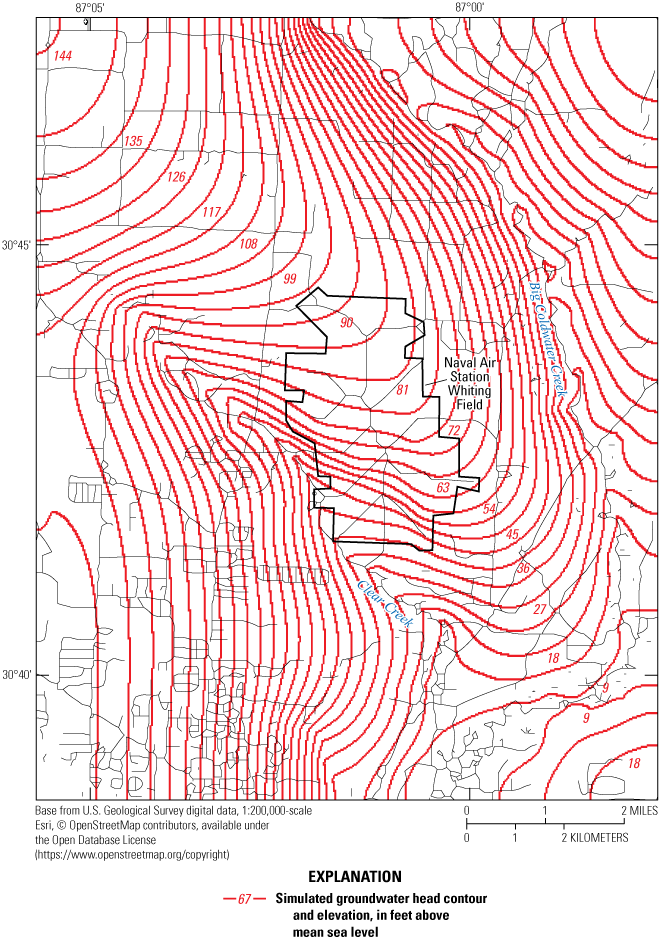
Vertically averaged simulated groundwater potentiometric contours in the Whiting Field groundwater model area, Naval Air Station Whiting Field, near Milton, Florida.
Comparison of measured and simulated heads at the 59 monitoring well locations shown in figure 12 indicates agreement is best at wells 2, 45, and 56, spread across Naval Air Station Whiting Field, and poorest at wells 50 and 36 to the southwest (table 10; fig. 25). Well 50 is less than 200 ft from Clear Creek and, along with wells 47, 48, and 49, indicates that groundwater in close proximity to the creeks may not be well represented at the scale of the model; however, well 45 is less than one-half of a mile from Clear Creek and is one of the locations where the simulation matched measured groundwater heads the best (table 10).
Table 10.
Measured and simulated groundwater heads at monitoring wells, Naval Air Station Whiting Field, near Milton, Florida.[ft, foot; amsl, above mean seal level]
| Map of numbered monitoring well (fig. 12) | Measured groundwater head (ft amsl) | Simulated groundwater head (ft amsl) | Residual (ft)1 |
|---|---|---|---|
| 1 | 44.34 | 47.31 | −2.97 |
| 2 | 74.73 | 74.69 | 0.04 |
| 3 | 74.87 | 74.72 | 0.15 |
| 4 | 74.92 | 74.75 | 0.17 |
| 5 | 75.07 | 74.77 | 0.3 |
| 6 | 77.19 | 74.81 | 2.38 |
| 7 | 74.58 | 74.27 | 0.31 |
| 8 | 74.87 | 74.68 | 0.19 |
| 9 | 75.17 | 74.94 | 0.23 |
| 10 | 75.18 | 74.94 | 0.24 |
| 11 | 67.3 | 67.66 | −0.36 |
| 12 | 67.72 | 67.99 | −0.27 |
| 13 | 61.83 | 63 | −1.17 |
| 14 | 64.75 | 66.14 | −1.39 |
| 15 | 59.31 | 57.83 | 1.48 |
| 16 | 61.54 | 59.1 | 2.44 |
| 17 | 62.76 | 62.32 | 0.44 |
| 18 | 61.33 | 63.28 | −1.95 |
| 19 | 57.68 | 55.92 | 1.76 |
| 20 | 60.51 | 61.83 | −1.32 |
| 21 | 49.3 | 51.47 | −2.17 |
| 22 | 49.29 | 52.13 | −2.84 |
| 23 | 49.9 | 52.18 | −2.28 |
| 24 | 63.72 | 64.5 | −0.78 |
| 25 | 54.63 | 52.42 | 2.21 |
| 26 | 75.47 | 72.8 | 2.67 |
| 27 | 78.28 | 77.46 | 0.82 |
| 28 | 75.01 | 73.88 | 1.13 |
| 29 | 76.34 | 75.57 | 0.77 |
| 30 | 73.75 | 73.96 | −0.21 |
| 31 | 78.51 | 78.1 | 0.41 |
| 32 | 80.56 | 78.62 | 1.94 |
| 33 | 42.09 | 42.44 | −0.35 |
| 34 | 45.44 | 44.35 | 1.09 |
| 35 | 45.66 | 44.23 | 1.43 |
| 36 | 47.74 | 43.27 | 4.47 |
| 37 | 41.77 | 40.65 | 1.12 |
| 38 | 41.77 | 40.67 | 1.1 |
| 39 | 41.8 | 40.69 | 1.11 |
| 40 | 41.89 | 41.51 | 0.38 |
| 41 | 47.18 | 43.44 | 3.74 |
| 42 | 47.14 | 43.41 | 3.73 |
| 43 | 37.99 | 40.05 | −2.06 |
| 44 | 38 | 40.05 | −2.05 |
| 45 | 46.72 | 46.79 | −0.07 |
| 46 | 46.93 | 46.84 | 0.09 |
| 47 | 39.27 | 42.22 | −2.95 |
| 48 | 40.07 | 43.43 | −3.36 |
| 49 | 40.2 | 43.5 | −3.3 |
| 50 | 36.06 | 41.13 | −5.07 |
| 51 | 62.02 | 60.34 | 1.68 |
| 52 | 61.86 | 61.04 | 0.82 |
| 53 | 62.66 | 62.77 | −0.11 |
| 54 | 78.73 | 77.93 | 0.8 |
| 55 | 78.72 | 78.23 | 0.49 |
| 56 | 77.87 | 77.8 | 0.07 |
| 57 | 79.35 | 78.48 | 0.87 |
| 58 | 68.99 | 69.24 | −0.25 |
| 59 | 68.79 | 69.05 | −0.26 |
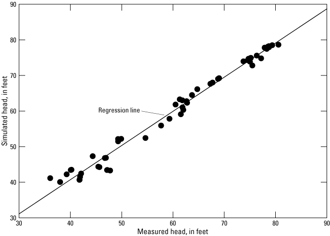
Plot of simulated versus measured groundwater heads, Naval Air Station Whiting Field, near Milton, Florida. [Regression coefficient is 0.98]
Unsaturated Zone Flow
Simulated surficial infiltration, in response to precipitation, is quite temporally variable, but the recharge from the unsaturated zone to the water table is steadier by comparison (fig. 26), starting at the steady-state values and rising slightly with the simulated surficial infiltration event of June 29–30, 2017. These simulations indicate that the deep unsaturated zone acts as a steady, long-term source of surficial infiltration to the sand and gravel aquifer. These simulation results are supported by the observed increase in the percentage of mobile water as depths to the water table increase (see “Hydrogeologic Properties” section).
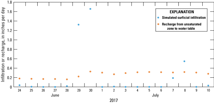
Plot of timeseries of groundwater model-area averaged simulated surficial infiltration and recharge from the unsaturated zone to the water table, Naval Air Station Whiting Field, near Milton, Florida.
Net recharge was calibrated in the steady-state model by matching flow at a USGS streamgage on Big Coldwater Creek (USGS station 02370500, fig. 10; U.S. Geological Survey, 2019). This effort yielded an average recharge rate of 61.5 inches per year (in/yr). With an average precipitation of 69.5 in/yr, this makes the losses that are due to interception storage and evapotranspiration in the unsaturated zone about 8.0 in/yr or 11.5 percent of precipitation.
Groundwater Discharge to Surface-Water Bodies
The simulated discharge of groundwater to the corresponding reaches of Clear Creek for discrete measurements of flow made on July 10, 2017, is listed in table 11. The field measurements and June 24–July 10, 2017, simulation results indicate more leakage to the creek in the reach from locations 2 to 3, which is closer to Naval Air Station Whiting Field, than leakage from locations 1 to 2. The simulated leakage is lower than measured values in both reaches, each by about 0.7 cubic foot per second (ft3/s), indicating the possibility of additional water, possibly runoff through the slough areas bordering Clear Creek.
Table 11.
Measured and computed groundwater leakage to Clear Creek on July 10, 2017, Naval Air Station Whiting Field, near Milton, Florida.[USGS, U.S. Geological Survey; ft3/s, cubic foot per second; NA, not applicable]
Groundwater Flow
The vertically averaged groundwater-flow vectors are generated from the binary cell-by-cell flow output from the model. The vectors indicate the dominance of Clear Creek and Big Coldwater Creek on groundwater flow in the WFGM system (fig. 27). Flow vectors proceed south over the northern and central parts of Naval Air Station Whiting Field and then southwest towards Clear Creek. Field measurements from 2018 were used to refine the benzene plume in the north-central plume (Alex Eddington, Resolutions Consultants, Inc., contracted to the U.S. Navy, unpub. data, 2020) resulting from contamination within Naval Air Station Whiting Field, and the path of the plume follows the simulated flow vectors (fig. 27). At the northern part of the plume, the flow-vector magnitudes are small and the highest benzene concentrations are detected in this relatively stagnant-flow area. Farther to the south and southeast, the plume moves towards Clear Creek by the higher groundwater-flow-vector magnitudes; moreover, it is interesting to note that the WFGM indicates that the north-south groundwater flow is about 1.38 ft3/s over the 8-mi east-west extent of the model area. In contrast, flow over the 10-mi by 8-mi model area is about 409 ft3/s, with an average net precipitation of 69.5 in/yr (U.S. Climate Data, 2019).
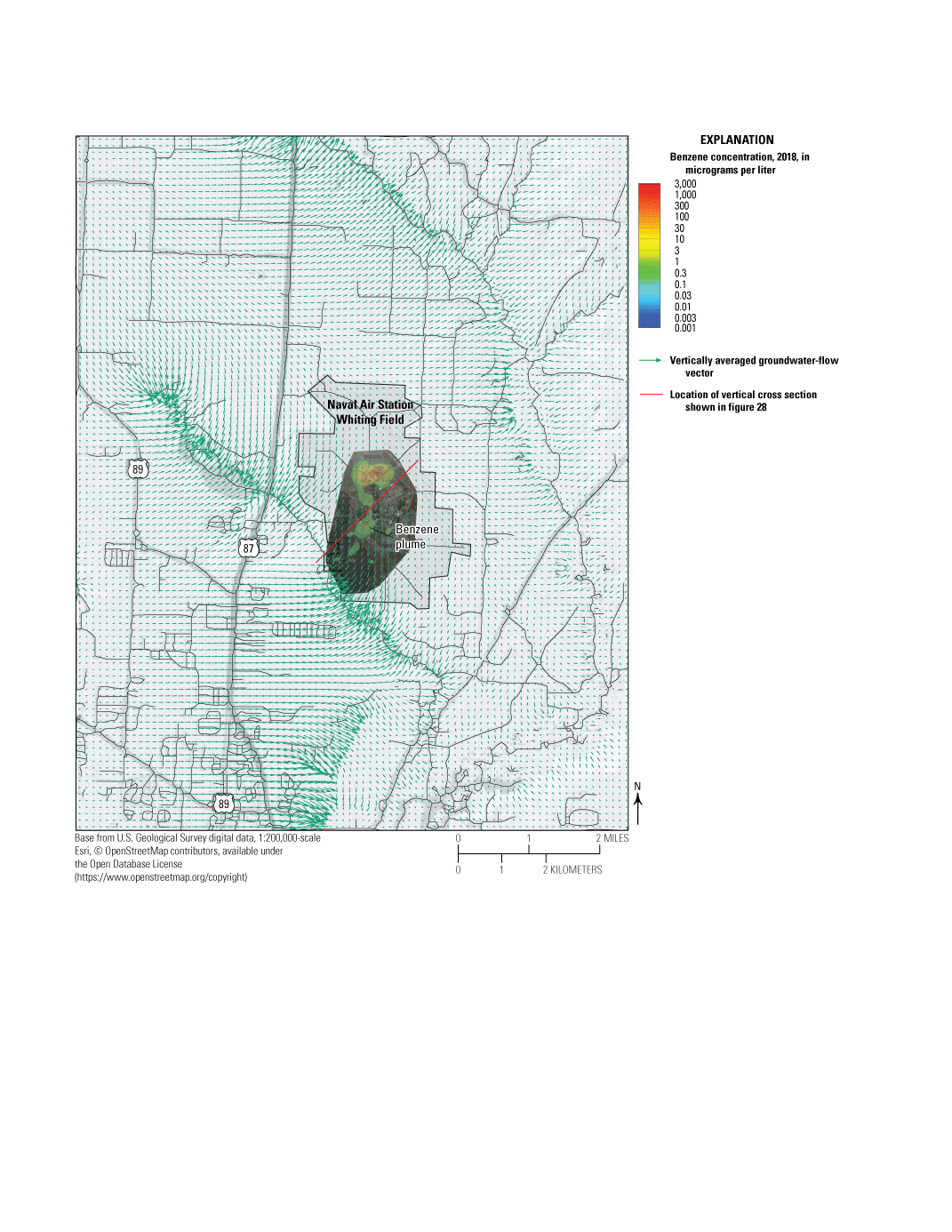
Vertically averaged groundwater-flow vectors from the steady-state Whiting Field groundwater model and measured benzene concentrations, north-central plume, 2018, Naval Air Station Whiting Field, near Milton, Florida. [Benzene data from Alex Eddington, Resolutions Consultants, Inc., contracted to the U.S. Navy, unpub. data (2020)]
The flow vectors in the vertical cross-section location shown in figure 28 indicate that the highest horizontal fluxes are in the lower depths of the aquifer beneath Naval Air Station Whiting Field. This cross-sectional view only documents flow magnitudes within the plane of the vertical cross section, so some of the increase in flow magnitude nearer to Clear Creek is due to the orientation of the main flow direction to the southeast. Recharge at the northeasternmost part of the vertical cross section may not proceed towards Clear Creek, and has some movement towards Big Coldwater Creek, but the part of the cross section corresponding to the benzene in the north-central plume location has flow vectors definitively towards Clear Creek. There does not seem to be substantial underflow across Clear Creek; flow from the west and the northeast is upward near the creek. This indicates that contamination plumes should largely flow into Clear Creek; however, extreme transient hydrologic events have not been simulated, and it is possible that underflow at Clear Creek might result from an unusual flow situation, such as intense precipitation over a small spatial extent on one side of the creek.
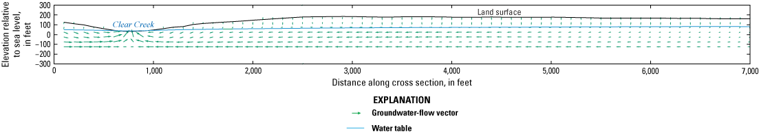
Groundwater-flow vectors within the plane of a vertical cross section from the steady-state Whiting Field groundwater model, Naval Air Station Whiting Field, near Milton, Florida. [Location of cross section shown in figure 27]
Assumptions and Limitations of Methods Used
The assumptions and limitations of the methods used revolve around those associated with the use of a model to simulate groundwater flow. The groundwater-flow model cell size affects the times of travel and can cause the times to be overestimated or underestimated depending on the location of the monitoring wells within the cells. The calibrated groundwater-flow model is one representation of the study area over the period simulated, and similar results could be achieved through different grid discretization, model boundary types or locations, and interpolation of model layering or hydraulic properties. However, the calibrated model is considered a reasonable solution.
Summary and Conclusions
Aviation-related activities have taken place at Naval Air Station Whiting Field, near Milton, Florida, since 1943. Benzene and trichloroethylene were detected in 1985 in samples of groundwater from two of three production wells that tap the sand and gravel aquifer at Naval Air Station Whiting Field. These detections are associated with the prior storage, use, and disposal of the chemicals required for the maintenance and repair of aircraft used at the site since 1943. Naval Air Station Whiting Field was placed on the U.S. Environmental Protection Agency Superfund program’s National Priorities List in 1994. Since then, the U.S. Navy Naval Facilities Engineering Systems Command Southeast has identified a north-central plume and a south-central plume in the sand and gravel aquifer.
In 2015, the U.S. Navy Naval Facilities Engineering Systems Command Southeast requested the U.S. Geological Survey collect additional data on the groundwater chemistry, hydrogeologic properties, and bioremediation potential of the sand and gravel aquifer near the north-central and south-central plumes and integrate previously existing and new data into a three-dimensional numerical model of groundwater flow at Naval Air Station Whiting Field.
Groundwater chemistry samples were collected in 2015 from eight existing monitoring wells along an uncontaminated groundwater-flow pathway across Naval Air Station Whiting Field. The field sampling results indicate groundwater in the uncontaminated part of the sand and gravel aquifer is acidic (pH between 4.62 and 6.24), dilute (specific conductance between 24 and 87 microsiemens per centimeter at 25 degrees Celsius), and oxic (dissolved oxygen concentrations between 1.87 and 6.44 milligrams per liter). Concentrations of the chlorofluorocarbons dichlorodifluoromethane and 1,1,2-Trichloro-1,2,2-trifluoroethane in the groundwater samples were analyzed for age-dating purposes but were detected in all samples at concentrations greater than those expected for past or modern air in equilibration with atmospheric water and indicate local sources. As such, these results could not be used for age dating. Concentrations of trichlorofluoromethane, however, were not greater than expected and indicate that groundwater along the groundwater-flow pathway recharged during the late 1970s to early 1980s.
Data related to the hydrogeologic properties of the sand and gravel aquifer were collected during 2017 and 2018 using natural gamma, electromagnetic induction (EMI), and borehole nuclear magnetic resonance (bNMR) borehole logging tools at seven monitoring wells proximal to the north-central and south-central plumes. Natural gamma and EMI logging data were used to noninvasively assess the vertical distribution of sands, gravels, and clays in the unsaturated and saturated zones of the sand and gravel aquifer. The bNMR logging provided novel data regarding the water content, percentage of mobile and immobile water, and most importantly, estimated hydraulic conductivity of the unsaturated and saturated aquifer formation materials. Average estimated hydraulic conductivities for the material assessed using the bNMR data ranged from 0.02 to 900 feet per day, and hydraulic conductivities generally increased with depth; these data support the fining upward geologic sequence related to the depositional history that had been determined by previous workers and natural gamma and EMI logs.
The bioremediation potential of the sand and gravel aquifer was assessed by the collection of aquifer formation material using vibracoring and rotosonic technology during the installation of three monitoring wells adjacent to the north-central and south-central plumes in 2018. The aquifer formation material was placed in microcosms in the laboratory and amended with radiocarbon (carbon-14), labeled as cis-1,2-Dichloroethylene with carbon-14 at the first and second carbons ([1,2-14C] cis-DCE). Under oxic conditions, [1,2-14C] cis-DCE was slowly transformed to carbon dioxide containing carbon-14 in all live microcosms for an average recovery of 20 percent. Microcosms under anoxic conditions also indicated transformation of [1,2-14C] cis-DCE to carbon dioxide containing carbon-14 for a slightly higher average of 28 percent. Combined, the microcosm experiments demonstrate that a substantial part of cis-1,2-Dichloroethylene loss observed in the north-central and south-central plumes during remedial investigations can be attributed to biological activity rather than hydrodynamic processes such as dispersion or dilution, and the mineralization to carbon dioxide explains the lack of vinyl chloride in the sand and gravel aquifer. Moreover, these experiments demonstrate the potential exists for dichloroethylene degradation in areas of the sand and gravel aquifer characterized by little to no dichloroethylene contamination.
A three-dimensional numerical groundwater-flow model of the sand and gravel aquifer was constructed for Naval Air Station Whiting Field and the surrounding area and calibrated for steady-state and transient conditions using historical groundwater heads, stream levels, baseflows, measured streamflows, and hydraulic conductivities determined from bNMR logging. The calibrated model reasonably reproduced measured groundwater heads and streamflows, while indicating groundwater-flow directions consistent with the locations of the north-central and south-central plumes. Moreover, the model can be used to run simulations of outcomes of potential remedial strategies, such as monitored natural attenuation, as part of future feasibility studies at Naval Air Station Whiting Field.
References Cited
Aeschbach-Hertig, W., El-Gamal, H., Wieser, M., and Palcsu, L., 2008, Modeling excess air and degassing in groundwater by equilibrium portioning with a gas phase: Water Resources Research, v. 44, no. 8, p. 1–12. [Also available at https://doi.org/10.1029/2007WR006454.]
Agency for Toxic Substances and Disease Registry, 2000, Public health assessment for Whiting Field Naval Air Station: Santa Rosa, Fla., U.S. Department of Health and Human Services, Public Health Service report, prepared by Federal Facilities Assessment Branch, Division of Health Assessment and Consultation, 72 p. [Also available at http://www.floridahealth.gov/environmental-health/hazardous-waste-sites/_documents/w/whitingfield091110.pdf.]
Allen, D., Flaum, C., Ramakrishnan, T.S., Bedford, J., Castelijns, K., Fairhurst, D., Gubelin, G., Heaton, N., Minh, C.C., Norville, M.A., Seim, M.R., Pritchard, T., and Ramamoorthy, R., 2000, Trends in NMR logging: Oilfield Review, v. 12, no. 3, art. OIREE70923–1730, 19 p., accessed July 3, 2018, at https://www.slb.com/~/media/Files/resources/oilfield_review/ors00/aut00/p2_19.pdf.
Asea Brown Boveri Environmental Services, Inc., 1998, Remedial investigation and feasibility study—General information report—Naval Air Station Whiting Field, Milton, Florida: North Charleston, S.C., Asea Brown Boveri Environmental Services, Inc., prepared for Department of the Navy, Southern Division, Naval Facilities Engineering Command, [variously paged].
Behroozmand, A.A., Keating, K., and Auken, E., 2015, A review of the principles and applications of the NMR technique for near-surface characterization: Surveys in Geophysics, v. 36, no. 1, p. 27–85. [Also available at https://doi.org/10.1007/s10712-014-9304-0.]
Bradley, P.M., 2003, History and ecology of chloroethene biodegradation—A review: Bioremediation Journal, v. 7, no. 2, p. 81–109. [Also available at https://doi.org/10.1080/713607980.]
Bradley, P.M., 2012, Microbial mineralization of cis-dichloroethene and vinyl chloride as a component of natural attenuation of chloroethene contaminants under conditions identified in the field as anoxic: U.S. Geological Survey Scientific Investigations Report 2012–5032, 30 p., accessed June 3, 2019, at https://doi.org/10.3133/sir20125032.
Busenberg, E., and Plummer, L.N., 1992, Use of chlorofluorocarbons (CCl3F and CCl2F2) as hydrologic tracers and age-dating tools—The alluvium and terrace system of central Oklahoma: Water Resources Research, v. 28, no. 9, p. 2257–2283. [Also available at https://doi.org/10.1029/92WR01263.]
Carr, M.B., Ehrlich, R., Bowers, M.C., and Howard, J.J., 1996, Correlation of porosity types derived from NMR data and thin section image analysis in a carbonate reservoir: Journal of Petroleum Science Engineering, v. 14, no. 3–4, p. 115–131. [Also available at https://doi.org/10.1016/0920-4105(95)00045-3.]
Casey, C.C., and Vroblesky, D.A., 2001, Characterizing the release and discharge of a contaminant plume using a numerical model, environmental tracers and water-to-vapor diffusion samplers, in 2001 International Containment & Remediation Technology Conference and Exhibition, Orlando, Florida, June 10–13, 2001, [Poster presentation]: Tallahassee, Fla., University of Florida.
Chapelle, F.H., Bradley, P.M., and Olsen, A., 2015, Sequential reducing/oxidizing conditions enhances natural attenuation at Naval Air Station Whiting Field: in Third International Symposium on Bioremediation and Sustainable Environmental Technologies, Miami, Florida, May 18–21, 2015, [Poster presentation]: Miami, Fla., Batelle Memorial Institute. [Also available at https://www.battelle.org/conference-proceedings/conference-proceedings.]
Coates, G.R., Xiao, L., and Prammer, M.G., 1999, NMR logging principles and applications: Houston, Tex., Halliburton Energy Services, 256 p. [Also available at https://books.google.com/books/about/NMR_Logging_Principles_and_Applications.html?id=vptTAAAAMAAJ.]
Florida Department of Environmental Protection, 2020, Factsheet about Outstanding Florida Waters (OFWs): Florida Department of Environmental Protection, 5 p., accessed August 11, 2020, at https://floridadep.gov/sites/default/files/OFW_factsheet.pdf.
Harbaugh, A.W., 2005, MODFLOW-2005—The U.S. Geological Survey modular ground-water model—The ground-water flow process: U.S. Geological Survey Techniques and Methods, book 6, chap. A16, [variously paged]. [Also available at https://doi.org/10.3133/tm6A16.]
Hayes, L.R., and Barr, D.E., 1983, Hydrogeology of the sand-and-gravel aquifer, southern Okaloosa and Walton Counties, northwest Florida: U.S. Geological Survey Water-Resources Investigation Report 82–4110, 49 p. [Also available at https://doi.org/10.3133/wri824110.]
Heaton, T.H.E., and Vogel, J.C., 1981, “Excess air” in groundwater: Journal of Hydrology (Amsterdam), v. 50, p. 201–216. [Also available at https://doi.org/10.1016/0022-1694(81)90070-6.]
Hȍhener, P., Werner, D., Balsiger, C., and Pasteris, G., 2002, Occurrence and fate of chlorofluorocarbon plumes in groundwater: Proceedings of the Groundwater Quality 2001 Conference, Sheffield, U.K., June 2001, IAHS Pub. no. 275, p. 41–47. [Also available at https://iahs.info/uploads/dms/12326.10-pp41-48-Hoehener--GQ69-.pdf.]
Im, J., Mack, E.E., Seger, E.S., and Lȍffler, F.E., 2019, Biotic and abiotic dehalogenation of 1,1,2-trichloro-1,2,2-trifluoroethane (CFC-113)—Implications for bacterial detoxification of chlorinated ethenes: Environmental Science & Technology, v. 53, no. 20, p. 11941–11948. [Also available at https://doi.org/10.1021/acs.est.9b04399.]
Jackson, R.E., Lesage, S., and Priddle, M.W., 1992, Estimating the fate and mobility of CFC-113 in groundwater—Results from the Gloucester landfill project, in Lesage, S., ed., Groundwater contamination and analysis at hazardous waste sites: New York, N.Y., CRC Press, p. 511–526. [Also available at https://www.routledge.com/Groundwater-Contamination-and-Analysis-at-Hazardous-Waste-Sites/Lesage/p/book/9780824787202.]
Keating, K., and Knight, R., 2012, The effect of spatial variation in surface relaxivity on nuclear magnetic resonance relaxation rates: Geophysics, v. 77, no. 5, p. E365–E377. [Also available at https://doi.org/10.1190/geo2011-0462.1.]
Kenyon, W.E., Day, P.I., Straley, C., and Willemsen, J.F., 1988, A three-part study of NMR longitudinal relaxation properties of water-saturated sandstones: Society of Petroleum Engineers Formation Evaluation, v. 3, no. 3, art. SPE–15643–PA, p. 622–636, accessed July 2018 at https://doi.org/10.2118/15643-PA.
Keys, W.S., 1990, Borehole geophysics applied to ground-water investigations: U.S. Geological Survey Techniques of Water-Resources Investigation, book 2, chap. E2, 150 p. [Also available at https://doi.org/10.3133/twri02E2.]
Landmeyer, J.E., and Wellborn, J.B., 2013, Geomorphology and groundwater origin of amphitheater-shaped gullies at Fort Gordon, Georgia, 2010–2012: U.S. Geological Survey Open-File Report 2013–1230, 19 p., accessed June 19, 2019, at https://doi.org/10.3133/ofr20131230.
Lesage, S., Jackson, R.E., Priddle, M.W., and Riemann, P.G., 1990, Occurrence and fate of organic solvent residues in anoxic groundwater at the Gloucester landfill, Canada: Environmental Science & Technology, v. 24, no. 4, p. 559–566. [Also available at https://doi.org/10.1021/es00074a016.]
Niswonger, R.G., Panday, S., and Ibaraki, M., 2011, MODFLOW-NWT, A Newton formulation for MODFLOW-2005: U.S. Geological Survey Techniques and Methods, book 6, chap. A37, 44 p. [Also available at https://doi.org/10.3133/tm6A37.]
Niswonger, R.G., Prudic, D.E., and Regan, R.S., 2006, Documentation of the Unsaturated-Zone Flow (UZF1) Package for modeling unsaturated flow between the land surface and the water table with MODFLOW-2005: U.S. Geological Survey Techniques and Methods, book 6, chap. A19, 62 p. [Also available at https://doi.org/10.3133/tm6A19.]
Plummer, N., and Friedman, L.C., 1999, Tracing and dating young ground water: U.S. Geological Survey Fact Sheet 134–99, 4 p. [Also available at https://doi.org/10.3133/fs13499.]
Shah, N., Nachabe, M., and Ross, M., 2007, Extinction depth and evapotranspiration from ground water under selected land covers: Ground Water, v. 45, no. 3, p. 329–338. [Also available at https://doi.org/10.1111/j.1745-6584.2007.00302.x.]
Swain, E.D., 2021, MODFLOW simulator used to assess groundwater flow for the Whiting Field Naval Air Station, Milton, FL: U.S. Geological Survey data release, https://doi.org/10.5066/P9M0OD8F.
Turnipseed, D.P., and Sauer, V.B., 2010, Discharge measurements at gaging stations: U.S. Geological Survey Techniques and Methods book 3, chap. A8, 87 p. [Also available at https://doi.org/10.3133/tm3A8.]
U.S. Climate Data, 2019, Milton weather averages: U.S. Climate Data digital data, accessed September 26, 2019, at https://www.usclimatedata.com/climate/milton/florida/united-states/usfl0323.
U.S. Geological Survey, 2017, USGS water data for the Nation: U.S. Geological Survey National Water Information System database, accessed August 8, 2017, at https://doi.org/10.5066/F7P55KJN.
U.S. Geological Survey, 2019, USGS water data for the Nation: U.S. Geological Survey National Water Information System database, accessed July 7, 2019, at https://doi.org/10.5066/F7P55KJN.
U.S. Geological Survey, 2020, USGS GeoLog Locator: U.S. Geological Survey database, accessed March 17, 2020, at https://doi.org/10.5066/F7X63KT0.
U.S. Geological Survey, [variously dated], National field manual for the collection of water-quality data: U.S. Geological Survey Techniques of Water-Resources Investigations, book 9, chaps. A1–A9, [variously paged], accessed January 12, 2018, at https://pubs.water.usgs.gov/twri9A.
U.S. Navy, 2012, Draft final remedial investigation report for Site 40, base-wide groundwater, Naval Air Station Whiting Field Milton, Florida: King of Prussia, Pa., U.S. Environmental Protection Agency ID no. FL2170023244, Contract task order JM40, prepared by Tetra Tech, [variously paged]. [Also available at https://prodenv.dep.state.fl.us/DepStaging/api/dms/5.187897.1.]
Walsh, D., Turner, P., Grunewald, E., Zhang, H., Butler, J.J., Jr., Reboulet, E., Knobbe, S., Christy, T., Lane, J.W., Jr., Johnson, C.D., Munday, T., and Fitzpatrick, A., 2013, A small-diameter NMR logging tool for groundwater investigations: Ground Water, v. 51, no. 6, p. 914–926. [Also available at https://doi.org/10.1111/gwat.12024.]
Weiss, R.F., 1970, The solubility of nitrogen, oxygen and argon in water and seawater: Deep-Sea Research, v. 17, p. 721–735. [Also available at https://www.sciencedirect.com/science/article/pii/0011747170900379.]
Williams, J.H., Lapham, W.W., and Barringer, T.H., 1993, Application of electromagnetic logging to contamination investigations in glacial sand and gravel aquifers: Ground Water Monitoring and Remediation, v. 13, no. 3, p. 129–138. [Also available at https://doi.org/10.1111/j.1745-6592.1993.tb00082.x.]
Conversion Factors
U.S. customary units to International System of Units
International System of Units to U.S. customary units
Temperature in degrees Celsius (°C) may be converted to degrees Fahrenheit (°F) as follows:
°F = (1.8 × °C) + 32.
Temperature in degrees Fahrenheit (°F) may be converted to degrees Celsius (°C) as follows:
°C = (°F − 32) / 1.8.
Datum
Horizontal coordinate information is referenced to the North American Datum of 1983 (NAD 83).
Vertical coordinate information is referenced to the National Geodetic Vertical Datum of 1929 (NGVD 29) or the North American Vertical Datum of 1988 (NAVD 88). Within the study area, altitude delta (NAVD 1988 minus NGVD 1929) ranges from −0.22 foot to the northwest to −0.15 foot to the southeast.
Altitude, as used in this report, refers to distance above the vertical datum.
Supplemental Information
Specific conductance is given in microsiemens per centimeter at 25 degrees Celsius (µS/cm at 25 °C).
Concentrations of chemical constituents in water are given either in milligrams per liter (mg/L), micrograms per liter (µg/L), picograms per kilogram (pg/kg; where 1 pg/kg is equivalent to 1.0×10⁻⁹ mg/L), millicuries per millimole (mCi/mmol), or millicuries (mCi).
Frequency measurements are given in kilohertz (kHz).
Abbreviations
amsl
above mean sea level [datum not specified]
bls
below land surface
bNMR
borehole nuclear magnetic resonance
CFC
chlorofluorocarbon
CFC-11
trichlorofluoromethane
CFC-12
dichlorodifluoromethane
CFC-113
1,1,2-Trichloro-1,2,2-trifluoroethane
CPMG
Carr-Purcell-Meiboom-Gill [sequence]
EMI
electromagnetic induction
EPA
U.S. Environmental Protection Agency
Ksdr
hydraulic conductivity estimated using the Schlumberger-Doll research equation
Ksoe
hydraulic conductivity estimated using the sum of echoes equation
PVC
polyvinyl chloride
Q
measurement of the coil resonance [dimensionless]
SDR
Schlumberger-Doll research [equation]
SOE
sum of echoes [equation]
Tr
relaxation time
T2
transverse relaxation time
UL
uniformly labeled
USGS
U.S. Geological Survey
WFGM
Whiting Field groundwater model
[1,2-14C] cis-DCE
cis-1,2-Dichloroethylene labeled with carbon-14 at the first and second carbons
3D
three dimensional
For more information about this publication, contact:
Director, U.S. Geological Survey
South Atlantic Water Science Center
1770 Corporate Drive
Suite 500
Norcross, GA 30093
678–924–6700
For additional information, visit: https://www.usgs.gov/centers/sa-water
Publishing support provided by the
Reston and Rolla Publishing Service Centers
Disclaimers
Any use of trade, firm, or product names is for descriptive purposes only and does not imply endorsement by the U.S. Government.
Although this information product, for the most part, is in the public domain, it also may contain copyrighted materials as noted in the text. Permission to reproduce copyrighted items must be secured from the copyright owner.
Suggested Citation
Landmeyer, J.E., Swain, E.D., Johnson, C.D., Lisle, J.T., McBride, W.S., Chung, D.H., and Singletary, M.A., 2021, Groundwater chemistry, hydrogeologic properties, bioremediation potential, and three-dimensional numerical simulation of the sand and gravel aquifer at Naval Air Station Whiting Field, near Milton, Florida, 2015–20: U.S. Geological Survey Scientific Investigations Report 2021–5124, 52 p., https://doi.org/10.3133/sir20215124.
ISSN: 2328-0328 (online)
Study Area
| Publication type | Report |
|---|---|
| Publication Subtype | USGS Numbered Series |
| Title | Groundwater chemistry, hydrogeologic properties, bioremediation potential, and three-dimensional numerical simulation of the sand and gravel aquifer at Naval Air Station Whiting Field, near Milton, Florida, 2015–20 |
| Series title | Scientific Investigations Report |
| Series number | 2021-5124 |
| DOI | 10.3133/sir20215124 |
| Publication Date | December 16, 2021 |
| Year Published | 2021 |
| Language | English |
| Publisher | U.S. Geological Survey |
| Publisher location | Reston, VA |
| Contributing office(s) | Caribbean Water Science Center, St. Petersburg Coastal and Marine Science Center, South Atlantic Water Science Center, WMA - Earth System Processes Division |
| Description | Report: xi, 52 p.; Data Release: Dataset |
| Country | United States |
| State | Florida |
| Other Geospatial | Naval Air Station Whiting Field |
| Online Only (Y/N) | Y |
| Additional Online Files (Y/N) | N |