

Kootenai River White Sturgeon (Acipenser transmontanus) Fine-Scale Habitat Selection and Preference, Kootenai River near Bonners Ferry, Idaho, 2017
Links
- Document: Report (4.8 MB pdf) , HTML , XML
- Data Release: USGS data release - White sturgeon fine-scale habitat model archive, Kootenai River near Bonners Ferry, Idaho, 2017
- Download citation as: RIS | Dublin Core
Acknowledgments
The U.S. Geological Survey would like to acknowledge and thank the partner agencies Idaho Department of Fish and Game, the Kootenai Tribe of Idaho, and the U.S. Army Corps of Engineers for assisting with data collection, data analysis, and support in developing this report. The authors would like to thank the members of the Kootenai River White Sturgeon Recovery Team who contributed to the conceptual framework and implementation of habitat-restoration projects and monitoring that were the foundation of this study. Finally, this report is dedicated to the memory of Paul Anders, who contributed immensely to the recovery of white sturgeon in the Kootenai River and throughout the Columbia River Basin.
Abstract
To quantify fine-scale Kootenai River white sturgeon (Acipenser transmontanus) staging and spawning habitat selection and preference within a recently restored reach of the Kootenai River, the U.S. Geological Survey, in cooperation with the U.S. Fish and Wildlife Service, integrated acoustic telemetry data with two-dimensional hydraulic model simulations within a 1.5-kilometer reach of the Kootenai River near Bonners Ferry, northern Idaho. Twenty-seven individual Kootenai River white sturgeon were detected in the study reach during May 6–June 30, 2017. The largest concentration of fish positions occurred near the edge of the gravel bar adjacent to the right bank pool-forming structure and additional concentrations of fish positions occurred near two recently constructed rock substrate clusters. The difference in preferred and available depth distributions quantifies that Kootenai River white sturgeon generally preferred depths of 7–11.5 meters, deeper than the most frequently available depths. About 71 percent of the detections occurred within the lower one-third of the water column, placing Kootenai River white sturgeon at or near the channel bed. The difference in available and preferred water velocities indicated that Kootenai River white sturgeon generally preferred a wide range of velocities from 0.0 to 1.0 meters per second, and generally preferred velocities that were less than the most frequently occurring available velocities. Kootenai River white sturgeon generally preferred the downstream part of the study area where water velocities were less than those in the upstream part. This study concludes that Kootenai River white sturgeon generally avoided shallow areas with increased velocities and generally favored deep areas with lower velocities near recently constructed restoration structures.
Introduction
Sturgeon (Acipenseridae) are a family of fish composed of 27 extant species that live in the ocean, estuaries, rivers, or inland waters of the Northern Hemisphere (Pikitch and others, 2005). Sturgeon are valued around the globe and harvested for their meat and roe (Pikitch and others, 2005). Over the last century, sturgeon populations have declined because of overharvesting, pollution, habitat degradation, or in some areas, a combination of each (Pikitch and others, 2005). The high demand for sturgeon, coupled with increasing anthropogenic effects within their natural habitat, caused a decline in sturgeon populations around the globe, with 85 percent of the family at risk of extinction (International Union for Conservation of Nature, 2020). White sturgeon (Acipenser transmontanus) are native to North America along the West Coast from Baja California to the Gulf of Alaska and inland throughout the Columbia, Fraser, and Sacramento River Basins (Pikitch and others, 2005). Generally large (commonly exceeding 2 meters [m]) and long-lived (as much as 100 years or more), white sturgeon mature slowly (15–30 years for adults) and reproduce infrequently (2–5 years between spawning events) (Pikitch and others, 2005; Kootenai Tribe of Idaho, 2010; Parsley and Kofoot, 2013). With recruitment failure in much of its range, Kootenai River white sturgeon share the same fate as many other sturgeon species around the globe, subjected to a combination of overharvesting, pollution, and habitat degradation. The limitation or elimination of sturgeon harvest and aquaculture programs using wild fish have helped sustain sturgeon populations but improvement of existing habitat may be needed to prevent extinction (Parsley and Kofoot, 2013).
Kootenai River white sturgeon are a genetically distinct and isolated white sturgeon sub-species endemic to the Kootenai River between Kootenay Lake in British Columbia and Kootenai Falls in northwestern Montana (U.S. Fish and Wildlife Service, 2008, 2019; Fisheries and Oceans Canada, 2014; fig. 1). Kootenai River white sturgeon are listed as endangered in the United States and Canada, in the Kootenai River and Kootenay Lake systems, respectively (U.S. Fish and Wildlife Service, 1994; Fisheries and Oceans Canada, 2014). The listing is the result of a wild fish population decrease in the late 1970s coupled with a near absence of natural recruitment. The population decrease and lack of natural recruitment is the result of a loss of suitable spawning habitat, reduced biological productivity, and water quality contamination (U.S. Fish and Wildlife Service, 2019). During spring, a select number of Kootenai River white sturgeon (hereinafter “Kootenai sturgeon”) migrate to, stage (as a reference to pre-spawn), and spawn within a 29.5-river kilometer (rkm) reach of the Kootenai River—a reach designated by the U.S. Fish and Wildlife Service as designated critical habitat for the species (U.S. Fish and Wildlife Service, 2008). Most Kootenai sturgeon spawn downstream from Bonners Ferry in areas with unsuitable spawning substrates composed of sand, silt, and clay (U.S. Fish and Wildlife Service, 2019; Parsley and Kofoot, 2013; Paragamian and others, 2009). Microhabitat where egg incubation and embryonic development may occur is an important factor in Kootenai sturgeon reproductive success (Parsley and Kofoot, 2013). Suitable spawning substrate consists of clean, smooth surfaces, and generally provides better incubation sites where the river hydraulics (increased velocity) maintain a clean substrate (Parsley and Kofoot, 2013). More suitable spawning substrates, consisting of boulders, cobbles, and gravel, are located at and upstream from Bonners Ferry; however, Kootenai sturgeon movement upstream from Bonners Ferry is minimal (Paragamian and others, 2009). The Idaho Department of Fish and Game (IDFG) has monitored adult Kootenai sturgeon movement within the Kootenai River in Idaho since the early 1990s and has identified and evaluated spawn timing and locations since 1994 using artificial substrate mats for egg collections. Kootenai sturgeon most frequently migrate to, stage, and spawn between river kilometer designations (rkm) 228 and 246 within the Kootenai sturgeon designated critical habitat (U.S. Fish and Wildlife Service, 2019; fig. 1). Kootenai sturgeon primarily spawn over or near substrates that ultimately lead to negligible natural recruitment (Parsley and Kofoot, 2013). Limited habitat complexity is thought to be the primary factor leading to the lack of natural recruitment (Kootenai Tribe of Idaho, 2010; U.S. Fish and Wildlife Service, 2019). Anthropogenic effects are visible and extend throughout the entire Kootenai sturgeon range. From the late 1800s through the mid-1900s, river-channel bank openings were closed along the main river channel by construction of a series of levees and dikes that extend from Kootenay Lake to a point upstream from Bonners Ferry. The dikes and levees, built upon natural levees, were designed to contain the natural peak flows to the main river channel prior to the completion of Libby Dam in December 1972. Drainage ditches equipped with sluicegates and pumps allow overbank seepage to drain or be pumped back to the main river, but also prevent floodplain interaction (Turney-High, 1969; Boundary County Historical Society, 1987; Redwing Naturalists, 1996).
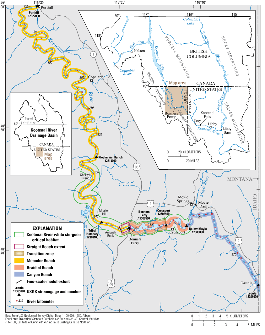
Location of the study area in the Kootenai River drainage basin, northern Idaho.
The completion of Libby Dam signified the beginning of a new, regulated flow regime for the Kootenai River that differed from the natural hydrograph in two ways—decreased annual peak flows and increased flows during the winter months (November–January; fig. 2). The regulated flow regime had an immediate effect on the habitat downstream from Libby Dam; decreased peak flow coupled with the dike construction all but eliminated floodplain connectivity. The sediment-trapping efficiency of Libby Dam virtually eliminated sediment contributions to the lower river except for tributary input between Libby Dam and the study reach (Fosness and Williams, 2009). The cooler water stored in Lake Koocanusa (impoundment formed by Libby Dam) for flood risk management and hydropower production contributes to cooler water in the spring and warmer water in winter (Beamesderfer and Anders, 2013). Each of these limiting-factor anthropogenic effects has degraded Kootenai sturgeon spawning habitat, not only within the designated critical habitat, but throughout their entire range (Kootenai Tribe of Idaho, 2010; U.S. Fish and Wildlife Service, 2019).
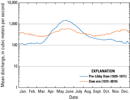
Kootenai River flow regime showing daily mean flow during pre-Libby Dam and Libby Dam eras, northern Idaho. Flow data are from U.S. Geological Survey streamgage 12305000 (Kootenai River at Leonia, Idaho; U.S. Geological Survey, 2021) for water years 1929–2019.
In 2010, the Kootenai Tribe of Idaho (KTOI) completed and began to implement their Kootenai River Habitat Restoration Program (KRHRP) Master Plan to restore and enhance the riverine and surrounding landscape and address limiting habitat factors with respect to focal species, including the endangered Kootenai sturgeon. Beginning in 2011, numerous KRHRP projects were constructed within the Kootenai River designated critical habitat. The projects addressed limiting factors to improve habitat conditions that support all life stages of endangered Kootenai sturgeon and other aquatic focal species. Targeted riverine limiting factors related to Kootenai sturgeon included (1) increasing habitat complexity using in-river features, (2) enhancing spawning habitat by providing rock substrates and increasing the hydraulic complexity, and (3) increasing pool habitat by constructing pool-forming features. Each targeted riverine habitat project was intended to provide a more suitable spawning substrate at and near known current spawning locations and enhanced habitat conditions that might entice Kootenai sturgeon to use areas upstream from Bonners Ferry where more suitable spawning substrates exist (Kootenai Tribe of Idaho, 2009).
This study, prepared in cooperation with the U.S. Fish and Wildlife Service, quantifies fine-scale Kootenai River white sturgeon staging and spawning habitat selection and preference within a recently restored, or treated, reach of the Kootenai River as described in the U.S. Fish and Wildlife recovery plan for the Kootenai River white sturgeon (U.S. Fish and Wildlife Service, 2019). Fine-scale acoustic telemetry positioning data were integrated with two-dimensional hydraulic model simulations to explain Kootenai sturgeon habitat preference at a fine scale (about 2 m) within a 1.5-kilometer (km) reach of the Kootenai River near Bonners Ferry, Idaho. In this study, we determined whether Kootenai sturgeon preferred habitat based on hydraulic flow characteristics, depth, and depth-averaged velocity. Depth and velocity have been used in previous studies to explain Kootenai sturgeon staging and spawning habitat, particularly in the Meander Reach (Paragamian and others, 2002, 2009; Paragamian and Duehr, 2005). Selected fish positions were paired with the depth and velocity data from the flow model to quantify habitat suitability. A cumulative habitat suitability index (HSI) and weighted usable area (WUA) describe the usable, or preferred, habitat area as a function of depth and velocity.
The methods and results of this study could be used in future investigations to (1) examine the fine-scale preference in staging and spawning locations for any years with fine-scale acoustic telemetry data, (2) simulate the two-dimensional streamflow to identify potentially suitable physical habitat in other reaches, and (3) inform future management actions regarding Kootenai sturgeon habitat-restoration projects and monitoring.
Study Area
The 780-km-long Kootenai River originates in the Canadian Rocky Mountains in British Columbia and is the second largest tributary to the Columbia River in terms of total annual streamflow volume. Flowing south into Montana, the river transitions into Lake Koocanusa, the upper Columbia River flood-storage reservoir formed by Libby Dam near Libby, Montana, under the Columbia River Treaty of 1964 (Northwest Power and Conservation Council, 1964). From Lake Koocanusa, the river flows through Libby Dam and west through a Canyon Reach into Idaho. About 7 miles upstream from Bonners Ferry, Idaho, the river transitions from a canyon to a wide, shallow, threaded gravel-and-cobble channel referred to as the Braided Reach. As the river approaches Bonners Ferry, Idaho, it transitions from the Braided Reach to a meandering channel near the Straight Reach, named for the approximately 1.5-km straight channel alignment through Bonners Ferry. From the Straight Reach, the river transitions to the Meander Reach, characterized predominantly by sand substrate in a meandering channel that continues downstream to Kootenay Lake (Snyder and Minshall, 1996; fig. 1).
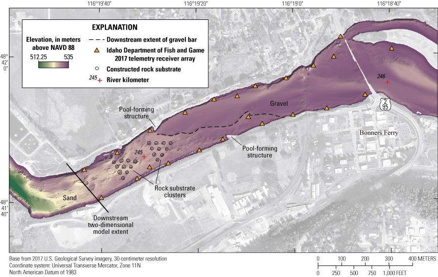
The study reach (rkm 244.7–246.2) includes the entire 1.5-km Straight Reach (fig. 1) and is located within a transition from free-flowing river upstream to backwater from Kootenay Lake. The transition to backwater, or “Transition Zone,” is variable throughout the year and generally ranges from the lower Straight Reach upstream into the Braided Reach (fig. 1). The Transition Zone generally is at the most downstream extent (rkm 244.7) in early spring concurrent with the lowest Kootenay Lake stage (water-surface elevation) and Kootenai River streamflow. The maximum backwater effect, often extending into the Braided Reach to near rkm 252.5, generally occurs during and after peak streamflow when Kootenay Lake is at or near full pool (generally May–July) (Berenbrock, 2005). The backwater transition also can be seen in the major transition in surficial sediment within the Straight Reach where the sediment transitions from gravel to sand. Previous bathymetric and sediment facies mapping efforts identified the lower part of the Straight Reach as a sediment transitional zone between gravel and sand (Barton and others, 2012). This sediment transitional zone is characterized by an abrupt shelf composed of gravel to a deeper thalweg generally consisting of sand (fig. 3). When the backwater is minimal, gravel is mobilized during high-flow events to the most downstream extent of the Transition Zone. The loss of energy owing to the backwater prevents gravel transport downstream, resulting in the sediment transition from gravel to sand (fig. 3; Barton and others, 2012).
Location of study extent in the Straight Reach, Kootenai River near Bonners Ferry, northern Idaho.
Historically, the Straight Reach was the most upstream Kootenai sturgeon staging and spawning reach based on data collected by IDFG (Paragamian and others, 2002; Rust and Wakkinen, 2009). The upper extent of the Straight Reach contains suitable Kootenai sturgeon spawning substrate, generally composed of gravel and cobble (Paragamian and others, 2002). In 2015, a river-restoration project was completed in the Straight Reach to add complexity to the channel and provide suitable Kootenai sturgeon staging and spawning habitat. Restoration treatment included a rock substrate “cluster” that provided a mix of gravel, cobble, and boulder substrate and added hydraulic complexities. Additionally, two pool-forming structures were added near the sediment transition to add or maintain depths and increase the hydraulic complexities (Kootenai Tribe of Idaho, 2011). For reasons still unknown, Kootenai sturgeon rarely stage and spawn upstream from the Highway 95 bridge (rkm 246; figs. 1, 3) at Bonners Ferry (Paragamian and others, 2009; U.S. Fish and Wildlife Service, 2019). Recent telemetry data collected by IDFG indicated Kootenai sturgeon movement upstream from the Highway 95 bridge, potentially the result of above-average streamflow conditions, flow-temperature mixing management, recent KTOI KRHRP restoration treatments, or a combination of each (Ross and others, 2018; Hardy and McDonnell, 2020; U.S. Fish and Wildlife Service, 2019). Based on egg collection mat (egg mat) data, Kootenai sturgeon selected the Straight Reach to stage and spawn, albeit at a lower frequency than other known spawning locations downstream (Paragamian and others, 2009; Ross and others, 2018, Hardy and McDonnell, 2020). In 2018, egg mats were deployed in the Braided Reach near a recently constructed KRHRP habitat project within rkm 246–250, and a single egg was collected on an egg mat, marking the first documented spawning event in the Braided Reach (Ryan Hardy, Idaho Department of Fish and Game, written commun., June 11, 2018). One recovery vision and strategy defined by the U.S. Fish and Wildlife Service (2019, p. 12) is “conducting research, monitoring, and evaluation” to determine the success and effectiveness of individual recovery objectives. The recent habitat-restoration treatments and IDFG fine-scale monitoring data within the Straight Reach provide a unique opportunity to describe fine-scale Kootenai sturgeon habitat selection and preference.
Methods
This project used multiple datasets to develop and combine two-dimensional hydraulic flow model (2D flow model) simulations with measured Kootenai sturgeon fish position (fish position) data collected in 2017. The 2D flow model results, combined with the fish position data, were summarized to describe the most frequently selected and preferred fine-scale habitat using Habitat Suitability Indices to determine a weighted usable area.
Defining and Differentiating Habitat Availability, Use, Selection, and Preference
Habitat terms are defined using definitions provided by Krausman (1999) and Litvaitis and others (1994) to differentiate how each is used within this study. “Habitat” is a general term that simply describes any area that could potentially be occupied by a species; in this case, all wetted areas of the Kootenai River physically accessible to Kootenai sturgeon are considered habitat. Habitat “availability” is a quantifiable metric describing measurable habitat characteristics such as depth and velocity. Habitat “use” describes a temporal and spatial association; for example, Kootenai sturgeon use the study reach for staging and spawning but may also use Kootenay Lake during other times of the year. Habitat “selection” implies a choice among alternative habitats that are available. For example, a part of the Kootenai sturgeon population selects the Straight Reach to stage and spawn; however, other fish may select different areas to stage and spawn. “Habitat preference” is determined independently of availability and can only be measured under the unique circumstances where continuous monitoring of the species provides data to summarize the frequency of selection. For example, Kootenai sturgeon are known to select the Straight Reach for staging and spawning based on IDFG movement monitoring and egg mat data. However, little can be inferred as to what habitat is most frequently selected within the Straight Reach using only coarse movement monitoring and egg mat data. Using acoustic telemetry data, a frequency of selection can be summarized. The telemetry data, paired with measurable habitat characteristics (depth and velocity), explained habitat in terms of preference. In short, habitat preference is the frequency of selection with respect to one or more habitat characteristics. The study reach contains a sudden habitat transition near the middle of the Straight Reach where the deeper areas and lower velocities within the Meander Reach transition to shallower areas with increased velocities common to and present throughout the Braided Reach. Depth and velocity were the habitat characteristics used in this study to quantify habitat based on depth and velocity preference.
Fine-Scale Acoustic Telemetry
IDFG used a VEMCO© positioning system (VPS) within the Straight Reach to produce fine-scale (about 2-m) Kootenai sturgeon positioning data. Beginning in 2003, ultrasonic transmitters (VEMCO© model V16), hereinafter referred to as “tags,” were surgically implanted in the abdominal cavities of Kootenai River white sturgeon. Beginning in 2014 and continuing each year thereafter, select Kootenai sturgeon had V16TP-6X tags implanted that recorded pressure (used to calculate depth with uncertainty of ±0.5 m) and temperature (Paragamian and Duehr, 2005; Ross and others, 2018). By 2017, a total of 108 adult females and 14 adult males in the Kootenai River drainage basin were tagged. Prior to the 2017 spawning season, 23 underwater acoustic VPS receivers (VR2 and VR2W) were placed in an array and staggered along the left and right banks (rkm 244.7–246.2) throughout the Straight Reach (Ross and others, 2018) (fig. 3). When tagged Kootenai sturgeon were in range, multiple receivers within the array received a signal, allowing the position to be triangulated to produce fine-scale Kootenai sturgeon positioning. However, individual Kootenai sturgeon do not spawn every year; therefore, only a subset of the total tagged individuals was detected in 2017. Fish positions were recorded at an irregular time-step interval, with the lowest recorded interval at 1 minute. Post-processed transmitter data included unique detection identification, date, time, latitude, and longitude. For each Kootenai sturgeon with a V16TP pressure sensor tag, depth and temperature data also were recorded. The horizontal position error (HPE), a dimensionless positional error estimate, was included for each fish position (Smith, 2013).
Random Positions
A random position dataset was created within the Straight Reach during the 2017 spawning season to help explain if the fish positions and resulting habitat preference occurred randomly rather than as a preferred process. The random position dataset was analogous to a fish preferring continuously random positions within the VPS array footprint (fig. 3). A randomized coordinate was generated for the same total count and temporal interval as the measured fish position data. The randomized coordinates were bound to the same spatial extent as the measured fish positions but positioned randomly within that extent, thus creating a randomized dataset to describe a random habitat preference.
Fine-Scale Physical Habitat
Multiple datasets were combined and integrated in a 2D flow model to summarize the fine-scale physical habitat. Real-time discharge and water-surface data were recorded at two U.S. Geological Survey (USGS) real-time streamgages (USGS streamgages 12310100 and 12309500; U.S. Geological Survey, 2021; fig. 1). Geometric terrain data included high-resolution topography (terrain above water surface) and bathymetry (terrain below water surface) collected in 2017. Topography data included topo-bathymetric Light Detection and Ranging (lidar), a technology that includes topography and the bathymetry (to about 3 m below the water surface for the Kootenai River data) (U.S. Geological Survey, 2017). Multibeam bathymetry data were collected in areas not covered by the topo-bathymetric lidar as part of a separate project in cooperation with the Kootenai Tribe of Idaho, with funding provided by Bonneville Power Administration (Fosness and Dudunake, 2019). Together, the lidar and multibeam bathymetry data provided a seamless high-resolution geometric terrain surface within the study reach. Acoustic Doppler current profiler (ADCP) streamflow velocity data were collected and provided measured velocity data within the reach in June 2017, near each of the artificial substrate clusters (Fosness, 2021).
Two-Dimensional Hydraulic Model
Kootenai River hydraulic conditions were simulated for the 2017 VPS fish position sample period (May 1–July 31, 2017) using the International River Interface Cooperative Flow and Sediment Transport with Morphological Evolution of Channels (FaSTMECH) two-dimensional hydraulic flow model (Nelson and others, 2003). In addition to this study, FaSTMECH 2D flow models were developed for numerous Kootenai River studies dating back to 2005. The methods used to develop, calibrate, and simulate FaSTMECH 2D flow models are described at length in multiple previous studies (Barton and others, 2005, 2009; Logan and others, 2011; McDonald and others, 2016; McDonald and Nelson, 2018, 2021; Fosness, 2021).
The 2D flow model extended from Ambush Rock (rkm 244.7) upstream to near Bonners Ferry (rkm 246.7). The 2D flow model extended 0.5 km upstream from the study reach to allow for a more suitable flow alignment. High-resolution (about 1-m) geometric terrain surface data (topography and bathymetry) were imported and used as the topography layer. Roughness coefficients describing the “roughness” of the channel bed originally were assigned based on a recent calibrated Kootenai River FaSTMECH 2D flow model (McDonald and Nelson, 2021); additionally, roughness coefficients were assigned to the bridge piers and KRHRP treatment features (rock substrate clusters and pool-forming structures). The computational grid included 2,000 grid points or “nodes” in the streamwise direction and 700 nodes in the cross-stream direction resulting in a 1-m by 1-m “fine-scale” grid. Model-boundary conditions required a downstream water-surface elevation (measured in meters) paired with a measured streamflow value measured in cubic meters per second. USGS streamgage Kootenai River at Tribal Hatchery (streamgage 12310100) provided instantaneous flow data (15-minute interval), and USGS streamgage Kootenai River at Bonners Ferry (streamgage 12309500) provided stage data verification within the study reach (fig. 1) (U.S. Geological Survey, 2021). Stage data were added to the streamgage datum offset, converting stage to water-surface elevation in North American Vertical Datum of 1988. The instantaneous flow and water-surface elevation data were averaged to an hourly time-step. Measured water-surface elevation data at the downstream boundary were not available at the fine-scale model downstream boundary (near Ambush Rock). A previously developed and calibrated FaSTMECH 2D flow model (McDonald and Nelson, 2018) was simulated on an hourly time-step for the same period (May 1–July 31) and provided the downstream water-surface elevation boundary condition for the fine-scale model.
The 2D flow model was calibrated over a series of steady-flow conditions representing a range of flow magnitudes (915, 978, 533, and 292 cubic meters per second [m3/s]) in 2017 (fig 4; Fosness, 2021). Model calibration generally included modifying the roughness drag coefficient values to minimize the root mean square error between the simulated water-surface elevations compared to measured water-surface elevations at the model calibration points. After calibration, the model was simulated at an hourly time-step during May 1–July 31, 2017, producing a total of 2,208 model simulations (fig. 4). The 2D model simulations were output for each hourly time-step and produced a unique solution that included depth (water-surface elevation minus bed elevation, in meters) and depth-averaged velocities (magnitude, measured in meters per second).
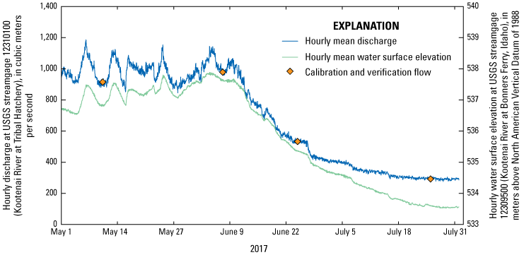
Two-dimensional flow model calibration and verification points during the spawning season in the Kootenai River study area, northern Idaho, May 1–July 31, 2017. USGS, U.S. Geological Survey.
Habitat Suitability Index Development
The 2D model output parameters (including depth and velocity) from the simulated flows were paired with measured fish, randomized, and available position data during the period of telemetry data to develop a dimensionless HSI for each parameter and position.
Because the fish positions did not always directly overlap with the model grid nodes (corner points of the grid), the measured fish positions were interpolated between the model grid nodes to provide estimated depth and velocity values for each fish position. The resulting values were compiled into depth and velocity distributions to quantify habitat preference with respect to the available hydraulic habitat conditions. The random positions were paired with the simulated values to determine if measured fish positions were a unique distribution compared to the random position distribution. The comparison between measured fish and randomized positions provided a method to determine if fish positions were random or selective. Distributions of selected depth and velocity at each measured and randomized fish position were determined by interpolating the simulated values at the corresponding time of each fish position. The available positions represent all model node data points within the footprint of the VPS. The available depth and velocity distributions were determined by extracting depth and velocity at each node within the VPS array for each 1-hour time-step. Two-sample Kolmogorov-Smirnov (K-S) goodness-of-fit tests were used to determine if significant differences existed between the distributions of available, selected, and randomized habitat.
The HSI provided a relative measure of habitat preference for each hydraulic parameter within the available area. To determine the HSI, the depth and velocity at each point first were weighted by the inverse of the available fraction within the area (areal fraction) using methods described in Wyman and others (2018). Depth and velocity are functions of discharge and backwater extent; therefore, the areal fraction of velocity and depth was unique for each model time-step. Habitat suitability distributions were developed by normalizing the weighted depth or velocity to obtain an HSI between 0 (least suitable) and 1 (most suitable). Assigning a weight to each parameter provided equal importance to areas where certain depths or velocities were preferred but were less available within the sample area. Moreover, the number of measured fish positions was variable for each fish; therefore, the HSI was weighted by the inverse of the fraction of individual positions to the total fish positions. Weighting the HSI by the inverse fraction of fish positions equalized the contribution of each fish for calculating habitat metrics to avoid any disproportionate effects on the results (Wyman and others, 2018).
Weighted Usable Area Index
The weighted usable area (WUA, in square meters) describes the available habitat based on habitat quality characterized from preferred habitat. This metric was calculated as
whereCHS
is the cumulative habitat suitability index value,
i
is the number of nodes in the two-dimensional flow model, and
ai
is the contributing area of the grid node.
Each grid node in the 2D flow model was given an HSI for depth and velocity based on the developed habitat suitability distributions from selected habitat. The CHS for each grid node in the model was calculated as the geometric mean of the depth and velocity HSI values. The WUA was calculated by multiplying the CHS by the contributing area of each grid node for a given discharge at a 1-hour time-step and summing all values. Like the HSI, the CHS is any value between 0 (least suitable) and 1 (most suitable). The WUA quantified the temporal changes in the preferred habitat as a function of discharge and variable backwater conditions that exist within the study reach. The CHS and WUA were calculated for the entire model area to distinguish temporal changes in habitat quality.
Kootenai River White Sturgeon Fine-Scale Habitat Selection and Preference
The 2017 spawning period consisted of an unusually early and extended-duration peak-discharge period (fig 4). Streamflow departed from the median daily statistic on March 19, and peak instantaneous flow of 1,260 m3/s (USGS streamgage 12310100, Kootenai River at Tribal Hatchery; U.S. Geological Survey, 2021) occurred on March 20, about 2 months earlier than the normal peak flow period (May/June). Flows remained at or greater than 766 m3/s through June 13. The above-average flow period was the result of above-average snowpack within the Kootenai River drainage basin. In mid-June, flow receded to less than the median daily statistic. Flows for the 2017 2D model and VPS fish position sample period (May 1 –July 31, 2017) ranged from a peak (maximum) of 1,186 m3/s on May 6 to a minimum of 276 m3/s on July 28 (fig 4). Because of the backwater from Kootenay Lake, the peak water-surface elevation at Bonners Ferry did not occur during the peak flow. The peak water-surface elevation of 537.9 m in the study reach occurred on June 4.
The available depths within the study reach summarize all wetted areas within the same extent of the VPS array. The depths for the spawning period were summarized by exporting the model results for each time-step and summarizing all the data. Available depths ranged from 0 to 11.76 m, with a mean depth of 5.85 m (±1.71 m) (table 1). Available depths generally were bimodal, with shallow areas in the upstream part of the study reach (about 5.6 m) and deeper areas in the downstream part of the study reach (about 9 m). Shallow areas (less than about 5.6 m) generally were located on gravel extending from the top of the reach to the downstream extent of the gravel bar (fig. 3). The deeper areas (more than 9 m) generally occurred in the lower one-half of the study reach downstream from the gravel bar, in the pools near the bridges, and on the right (north) side of the river (fig. 5A).
Table 1.
Depth and velocity summary for available, selected, and random habitat from hydrodynamic model simulations, Kootenai River study area, northern Idaho, 2017.[Available habitat: Summarized for each model simulation within the telemetry footprint on an hourly time-step for May 5–June 30, 2017. Selected habitat: For a total of 42,267 fish locations from 27 individual fish, May 5–June 30, 2017. Random habitat: Random positions, generated at 42,267 locations. Abbreviations and symbol: SD, Standard deviation; min, minimum; max, maximum; ±, plus or minus]
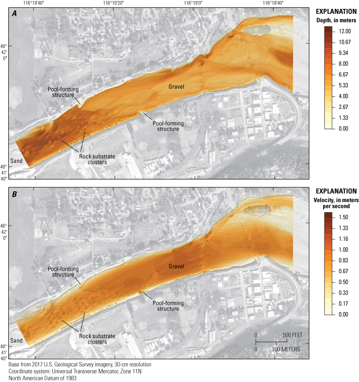
Example International River Interface Cooperative Flow and Sediment Transport with Morphological Evolution of Channels two-dimensional hydraulic flow model with (A) example depth and (B) velocity, Kootenai River study area, northern Idaho, June 6, 2017.
The available depth-averaged velocities in the study reach were summarized using the same methods described for the depth data and ranged from 0 to 1.47 meters per second (m/s) (table 1). The mean and median velocity in the study reach were 0.86 m/s (±0.26 m) and 0.91 m/s, respectively. The highway and railroad bridges are located at a natural contraction in the river, and the reduction in width in conjunction with shallower depths increased depth-averaged velocities within the contracted area. In contrast, the sudden increase in depth downstream from the gravel bar caused a sudden decrease in the velocities.
Measured Kootenai Sturgeon Fish Positions
In 2017, 54 tagged adult Kootenai sturgeon were detected in the Idaho part of the Kootenai River (Hardy and McDonnell, 2020). Of the 54 adult Kootenai sturgeon, 27 individuals (23 females and 4 males) were detected in the study reach. At the time of tagging (2009–17), fish fork length ranged from 151 to 269 centimeters and weights ranged from 26 to 81 kilograms. The first tagged Kootenai sturgeon was detected in the study reach on May 6, 2017, and the last detection was on June 30, 2017. A total of 49,501 Kootenai sturgeon position detections (Kootenai sturgeon or fish positions) were recorded. The HPE values (dimensionless) ranged from a minimum of 9.1 to a maximum of 336.9, where the maximum value was too large for a fine-scale analysis. Numerous fish positions were located outside of wetted area (on the land surface). The HPE of these positions was reviewed and generally was larger than 12, indicating, therefore, that fish positions with an HPE greater than 12 were too coarse to be included in this fine-scale study. After filtering the HPE to 12 and less, a total of 42,267 fish positions were used for the analysis (fig. 6). Of the total fish positions used in this analysis, 48 percent were from a single fish; HSI values were weighted to remove the disproportionate effect of that individual using methods described in Wyman and others (2018).
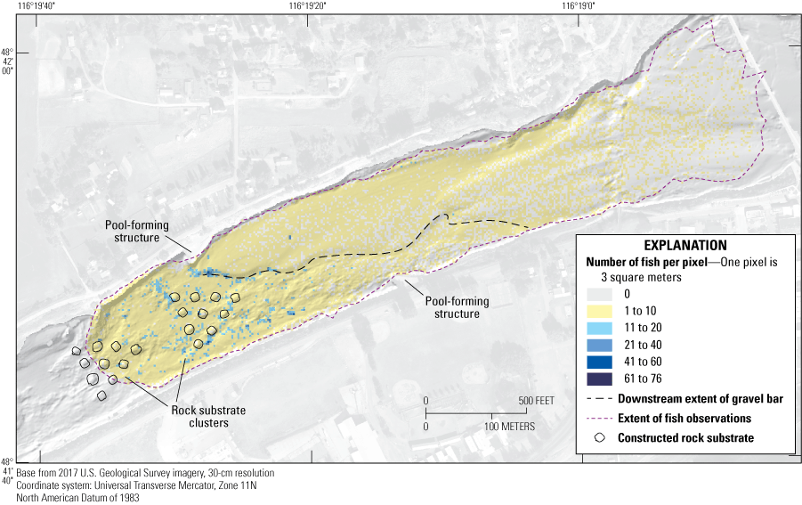
Kootenai River white sturgeon fish positions, Kootenai River near Bonners Ferry, northern Idaho, May 6–June 30, 2017.
Kootenai sturgeon observations predominantly occurred downstream from the gravel bar extent (figs. 3, 6). The largest concentration of observations occurred near the edge of the gravel bar adjacent to the right bank (north) pool-forming structure; three additional areas with large concentrations of measured fish positions occurred near the two rock substrate clusters. Only two locations with more than 10 measured fish positions occurred upstream from the gravel bar extent (fig. 6). The ADCP data collected on June 6, 2017, described the three-dimensional depth and velocity variability near the areas with the largest concentration of fish observations. For areas directly downstream from the edge of the gravel bar and substrate clusters, the ADCP data provided a visual representation of the velocities near substrate clusters (fig. 7; Fosness, 2021). The ADCP velocity data are not captured in the area near the water surface. This area is referred to as the blanking distance and, for the ADCP used in this study, results in missing data of about 0.5 m. Additionally, velocity data near the channel bed (lower 6 percent of the water depth) also are unable to be measured (Mueller and others, 2013).
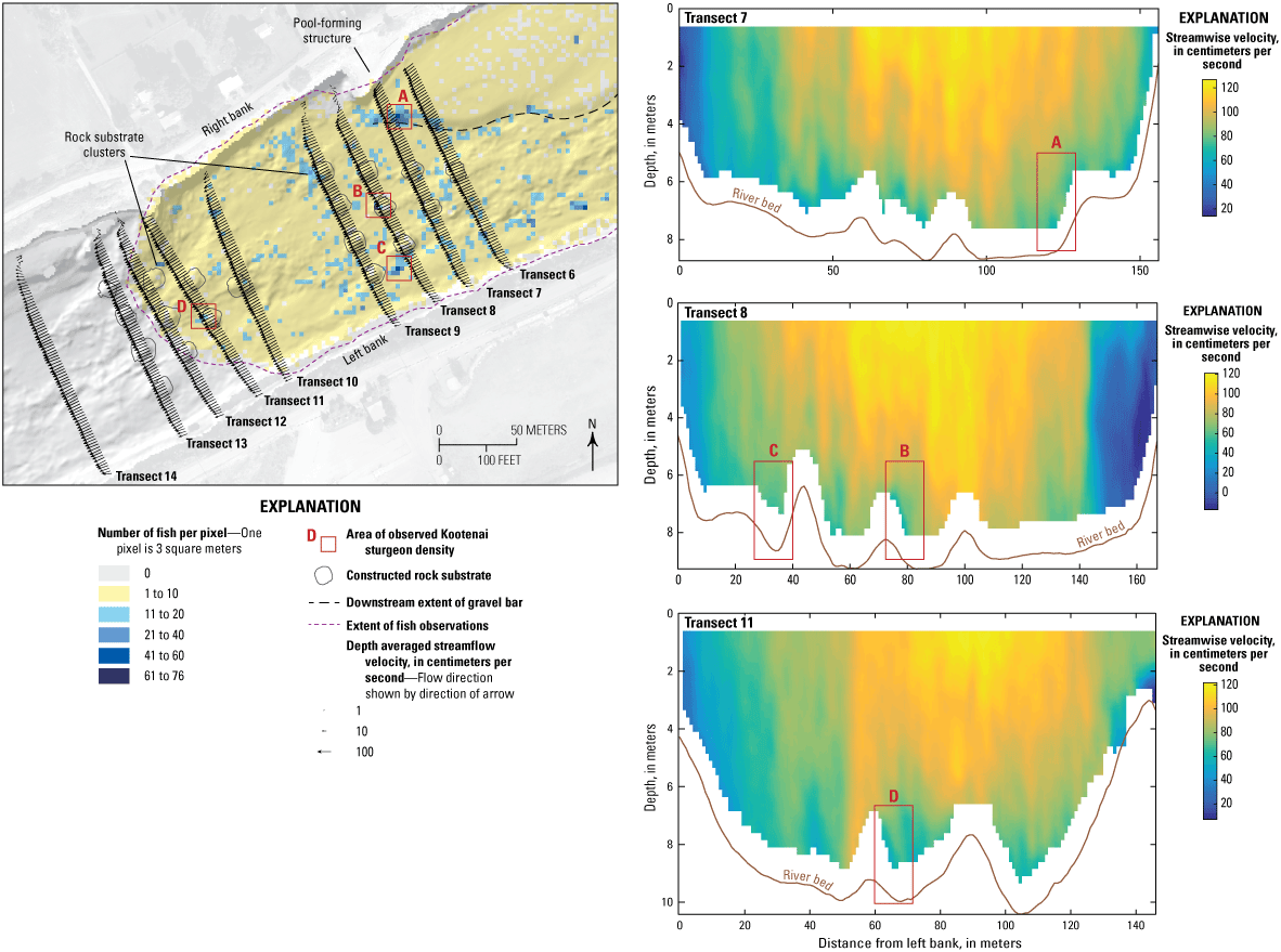
Acoustic Doppler current profiler data and Kootenai River white sturgeon fish positions near the Kootenai River Habitat Restoration Project sites, northern Idaho, June 6, 2017.
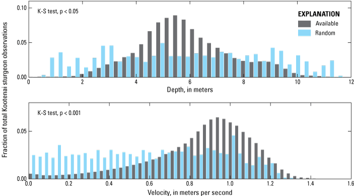
Measured fish position depths, hereinafter described as “selected depths,” ranged from 0.28 to 11.47 m, with a mean depth of about 7 m (±1.8 m). To clarify, the measured fish position depths are stated using the fish position combined with the 2D model depths. In comparison, the available depths had about the same range, but overall were shallower, with an average of 5.85 m (fig. 8). Two peaks in available depths occurred, around 5.5 and 9 m, whereas the Kootenai sturgeon most frequently preferred depths from 7 to 11.5 m. The bimodality of available depths at 5.5 and 9 m represent shallow gravel substrates and deeper sandy substrates mixed with intermittent gravels, respectively. A K-S test compared the similarity between the preferred and available distributions. The K-S test resulted in a low p-value (probability that these data would have occurred by random chance) of less than 0.05, rejecting the null hypothesis that the distribution between the preferred and available depths are from the same distribution. The difference in preferred and available depth distributions objectively quantifies that Kootenai sturgeon generally preferred depths of 7–11.5 m, deeper than the most frequently available depths.
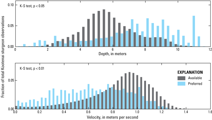
Fraction of total Kootenai River white sturgeon depth and velocity observations for available and preferred fish positions, Kootenai River near Bonners Ferry, northern Idaho. K-S test, Kolmogorov-Smirnov test; p <, probability that these data would have occurred by random chance is less than.
Measured fish position velocities, hereinafter referred to as “selected velocities,” ranged from about 0 to 1.27 m/s with an average velocity of about 0.8 m/s (±0.24 m/s). Kootenai sturgeon preferred a wide range of velocities from 0.0 to 1.0 m/s. The available velocities ranged from 0 to 1.47 m/s, with a mean of 0.86 m/s. (fig. 8). The K-S test resulted in a low p-value (<0.01), therefore rejecting the null hypothesis that the preferred and available velocities are from the same distribution. The difference in available and preferred velocities indicates that Kootenai sturgeon generally preferred a wide range of velocities from 0.0 to 1.0 m/s and generally preferred velocities that were less than the most frequently occurring available velocities.
Four Kootenai sturgeon with V16TP sensors were measured in the study reach in 2017. Depth data from the four Kootenai sturgeon were compared to model output depths (total depth) based on the fish position. Using 707 depth observations, about 71 percent of the detections occurred within the lower one-third of the water column (fig. 9). Thirty Kootenai sturgeon depth observations exceeded the total depth, indicating an error in the positions resulting in an erroneous depth estimate. For those 30 detections, the Kootenai sturgeon presumably were at or near the channel bed. These findings align with a previous study reporting that about 75 percent of the Kootenai sturgeon occupied the lower one-third of the water column during the staging and spawning periods (Paragamian and Duehr, 2005). A depth preference for the lower one-third of the water column is shown along with the velocities near the largest concentration of observations at transects 7, 8, and 11 (fig. 7).
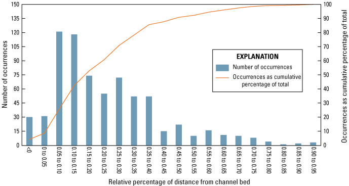
Measured Kootenai River white sturgeon depths compared to model simulation total depth for 707 observations in the Kootenai River near Bonners Ferry, northern Idaho, 2017.
Random Positions
Random coordinate positions were generated for 42,267 positions, the same as the measured fish positions. The random positions were set to the same time-step interval as the measured fish positions to ensure that the two datasets were similar in total counts and temporal interval and were paired with 2D flow model output data using the same methods described for the measured fish positions and summarized in terms of depth and velocity.
Random position depth and velocity distributions simulated random fish selection within the VPS array footprint. The random distributions provided a comparison to the available depth and velocity distributions and were uniformly distributed in depths ranging from 0 to 11.41 m and velocities ranging from 0 to 1.43 m/s within the VPS array. Although the random position depth distribution was uniformly distributed (fig. 10), the random depth fraction exceeded the available depth fraction for depths of 0 to about 3 m and 8 to 11.41 m. The random depth distribution was not the same as the available depth distribution (K-S test, p <0.05), indicating that randomly selected depths are not a function of the available depths and that a broad depth range was available. The random velocities (fig. 10) exceeded the available velocities for values ranging from 0 to about 0.7 m/s. The random velocity distribution was not the same as the available velocity distribution (K-S test, p <0.001). More spatial area was available for velocities of about 0.7–1.43 m/s, but an equal opportunity for the full range of velocities, if preferred.
Kootenai River white sturgeon depth and velocity for available and random positions, Kootenai River near Bonners Ferry, northern Idaho. K-S test, Kolmogorov-Smirnov test; p <, probability that these data would have occurred by random chance is less than.
Random depth and velocity distributions were compared to the preferred depth and velocity distributions to quantify preference as a random or systematic distribution. There was a significant difference (K-S test, p <0.01) between preferred and random depth distributions, suggesting that specific depths were preferred (fig. 11). Although fish observations occurred at nearly all depths, fish preferred depths greater than about 7.5 m. Random and selected velocity distributions were compared to determine if fish preferred certain velocities in the study area. The K-S test indicated the distributions were similar (p >0.5); therefore, the velocity preference aligns with a random process (fig. 11).
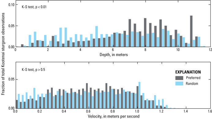
Kootenai River white sturgeon depth and velocity for random and selected fish positions, Kootenai River near Bonners Ferry, Idaho,
Habitat Suitability Indices
Habitat suitability indices (HSIs) were developed by pairing selected fish positions with depths and velocities from the flow model to determine habitat preference in the study reach. HSI values were calculated by normalizing the depth and velocity values by fish position counts to avoid one fish having a disproportionate effect on the habitat suitability curve. Depth bins ranged from 0 to 11 m (with the largest preference ranging from 8 to 9 m) and represented 18 percent of the total normalized weighted count of fish observations. Depth HSI was limited to a narrow selection of depths from 6 to 9 m (fig. 12; Fosness, 2021).
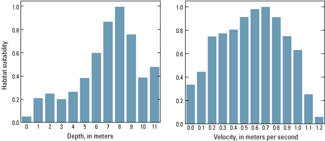
Kootenai River white sturgeon depth and velocity habitat suitability indices, Kootenai River near Bonners Ferry, northern Idaho.
Velocity bins ranged from 0.0 to 1.2 m/s (with the highest preference ranging from 0.6 to 0.8 m/s) and represented 12 percent of the total normalized weighted count of fish observations. Most velocity HSI values were distributed from 0.2 to 1.0 m/s. The wide band of velocity HSI resulted in a geometric mean value that is evenly distributed across the range of velocities (fig. 12; Fosness, 2021).
The CHS was calculated using the geometric mean of depth and velocity HSI results. The CHS was highest near the channel thalweg and rock substrate clusters, where the local depths and velocities ranged from 6 to 9 m and 0.2 to 1.0 m/s (figs. 5, 13), respectively. The CHS generally decreased upstream from the gravel bar shelf where depths were shallow, resulting in increased velocities. One exception to the decreased CHS upstream from the gravel bar was the deeper area near the right bank immediately downstream from the railroad bridge where the velocities were lower (fig. 13).
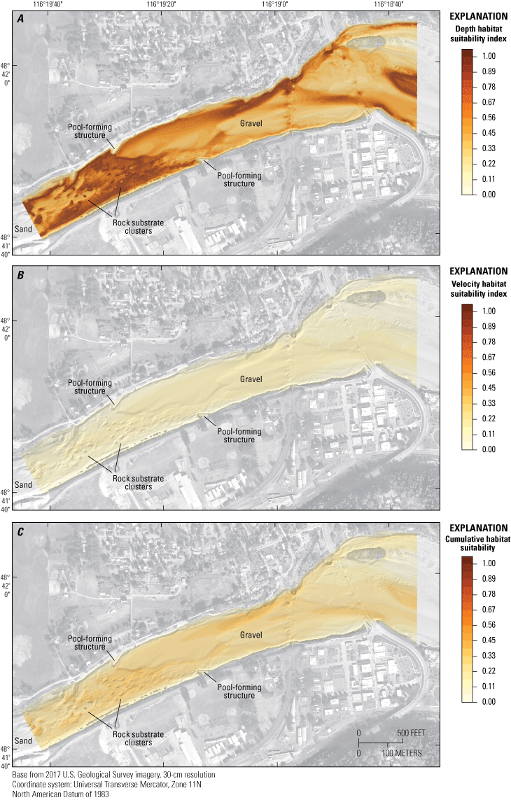
Kootenai River white sturgeon habitat suitability, at Kootenai River near Bonners Ferry, northern Idaho, on May 6, 2017, at 5:00 p.m. Habitat suitability indices for depth (A) and velocity (B) are on a scale of 0–1 (1=highest suitability). Cumulative habitat suitability (C) was calculated as the geometric mean of the depth and velocity habitat suitability indices.
Weighted Usable Area
The WUA describes the usable, or preferred, habitat area as a function of temporally variable parameters, including depth and velocity. Discharge, in addition to the variable backwater within the Transition Zone, created a continuously variable WUA throughout the model period. The WUA ranged from about 34,300 to 72,900 m2 and generally was explained by the total discharge in the study reach (275–1,190 m3/s) (fig. 14; Fosness, 2021). The WUA generally followed the same trends as discharge, indicating a positive relation between the habitat quality and increased discharge based on CHS metrics. One exception was that the maximum WUA did not occur during the peak flow on May 6. The maximum WUA (73,900 m2) occurred during the peak water-surface elevation on June 4, the result of increased depth because of the increased backwater from Kootenay Lake (fig. 14). In comparison, the WUA during the peak flow (1,190 m3/s) on May 6 was seven percent lower (67,700 m2) because of the lower extent of backwater from Kootenay Lake (fig. 14).
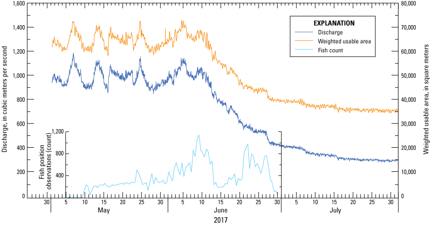
Weighted usable area and discharge of Kootenai River white sturgeon habitat in the study extent, Kootenai River near Bonners Ferry, northern Idaho, May–July 2017.
Peak fish observations occurred on June 9 (1,143 observations), with a secondary peak occurring on June 22 (974 observations) (fig. 14). The June 9 peak occurred 5 days after the maximum WUA. However, a second peak fish observation occurred on June 22, when the WUA was 57 percent lower than the maximum WUA.
Considerations for Future Habitat Studies
Future investigations might consider applying methods from this study to identify the potential for preferred physical habitat in additional reaches of the Kootenai River or other white sturgeon reaches outside the Kootenai River. The methods and results of this study could be further expanded to inform future management actions regarding (1) the seasonal flow and stage regime and (2) Kootenai sturgeon habitat-restoration projects and monitoring. The 2D model data could be simulated in near real-time to identify what forecasted conditions may provide with respect to WUA. For example, the Northwest River Forecast Center provides 10- and 120-day forecasts for stage and streamflow. For the Kootenai River, stage and streamflow are predominantly dependent on conditions from Kootenay Lake (stage and resulting backwater) and outflow from Libby Dam (streamflow). The 2D model could simulate the forecasted stage and streamflow combinations and provide a daily WUA within the forecasted period. The resulting WUA results would provide water and biological managers with a tool to support flow timing and duration. The methods of this study also could be used to identify Kootenai sturgeon habitat-restoration projects and monitoring by considering the WUA within the habitat-restoration and monitoring designs. For example, habitat treatments could be assessed to ensure that a desired amount of WUA is achieved based on the design criteria. Monitoring efforts could target areas that have been identified as having the largest potential WUA and, therefore, the highest likelihood of fish position observations.
Discussion
An above-average snowpack within the Kootenai River drainage basin in 2017 resulted in an above-average flow period on the Kootenai River with an early and extended duration peak-flow period. The IDFG suggested that the number of days where flow exceeds 850 m3/s might be the best predicator of probability of Kootenai sturgeon migration into the braided reach (Hardy and McDonnell, 2020). Of the 54 tagged adult Kootenai sturgeon, 27 were detected in the study reach during May 6–June 30, 2017, indicating that the above-average flow period may have increased the number of Kootenai sturgeon in the study reach. After filtering the fish position data to include positions with a horizontal position error of 12 or less, a total of 42,267 Kootenai sturgeon position detections were used in the analysis. Kootenai sturgeon observations predominantly occurred downstream from the gravel bar extent. The largest concentration of observations occurred near the edge of the gravel bar adjacent to the right bank (north) pool-forming structure and in three additional areas with large concentrations of measured fish positions near the two rock substrate clusters. The fish position spatial locations used in this study generally agreed with those from Golder Associates Limited (2020); however, the objectives for this study related fish positions to the selected depth and velocity to explain habitat selection and preference.
The difference in preferred and available depth distributions quantifies that Kootenai sturgeon generally preferred depths of 7 to 11.5 meters (m), deeper than the most frequently available depths. Kootenai sturgeon observations predominantly occurred downstream from the gravel bar extent, and about 71 percent of the fish position detections with depth-tags occurred within the lower one-third of the water column, placing Kootenai sturgeon at or near the channel bed. This observation agrees with findings from Paragamian and others (2009) in which 75 percent of the positions also were within the lower one-third of the water column.
The difference in available and preferred velocities indicated that Kootenai sturgeon generally preferred locations with a wide range of velocities from 0.0 to 1.0 m/s and generally preferred areas where the depth-averaged velocities were less than the most frequently occurring available depth-averaged velocities. However, given that Kootenai sturgeon were in the study reach during the peak backwater conditions, the velocity variability within the reach was minimal. Kootenai sturgeon generally preferred the downstream part of the study area where velocity was less than in the upstream part. Paragamian and others (2009, p. 640) noted that Kootenai sturgeon spawn “in areas of highest available velocity and depths over a range of flow.” This suggestion may be valid for the Meander Reach critical habitat, but the results of this study suggest that Kootenai sturgeon preferred deep areas with decreased velocities (downstream from gravel bar and near recently constructed substrate clusters).
A random position dataset was created within the Straight Reach during the 2017 spawning season to help explain if the fish positions and resulting habitat preference occurred randomly rather than as a preferred process. The randomized coordinates were bound to the same spatial extent as the measured fish positions but were positioned randomly within that extent, thus creating a randomized dataset intended to describe a random habitat preference. The random depth distribution was not the same as the available depth distribution (K-S test, p < 0.05), indicating that randomly selected depths are not a function of the available depths and that a broad depth range was available, if preferred. The random velocity distribution was not the same as the available velocity distribution (K-S test, p <0.001), indicating more spatial area available where velocities were about 0.7–1.43 m/s but an equal opportunity for the full range of velocities, if preferred.
In contrast to the available area, random depth and velocity distributions were compared to the preferred depth and velocity distributions to quantify preference as a random or systematic distribution. The preferred and random depth distributions differed significantly (K-S test, p < 0.01), suggesting that specific depths were preferred. Although fish observations occurred at nearly all depths, fish preferred depths greater than about 7.5 m. Random and selected velocity distributions were compared to determine if fish preferred certain velocities in the study area. The K-S test indicated that the random and selected velocity distributions were similar (p >0.5); therefore, the velocity preference aligned with a random process. Perrin and others (2003) suggested that hydraulically complex areas are used for spawning in a confined river channel for unregulated and regulated rivers. A depth-averaged velocity might not sufficiently explain velocity near areas with rapidly changing hydraulic complexity, such as those immediately downstream from the gravel bar and near the substrate clusters. Using a three-dimensional model near preferred areas (downstream from the gravel bar and near recently constructed substrate clusters) may more accurately explain the hydraulic complexity in the lower one-third of the water column.
The depth habitat suitability index (HSI) was limited to a narrow selection of depths ranging from 6 to 9 m, whereas velocity HSI values were more widely distributed, ranging from 0.2 to 1.0 m/s. The wide band of velocity HSI results in a geometric mean value that was evenly distributed across the range of velocities. The cumulative habitat suitability (CHS) was highest near the channel thalweg and rock substrate clusters where the local depths and velocities ranged from 6 to 9 m and from 0.2 to 1.0 m/s, respectively. The CHS generally decreased upstream from the gravel bar shelf where depths were shallow resulting in increased velocities. One exception to this pattern was near the right bank immediately downstream from the railroad bridge, where depths and velocities increased.
The weighted unit area (WUA) generally followed the same trends as discharge, indicating a positive relation between the habitat quality and increased discharge based on CHS metrics. However, the maximum WUA did not occur during the peak flow on May 6 but rather during the peak water-surface elevation on June 4, the result of increased depth owing to the increased backwater from Kootenay Lake. Peak fish observations occurred on June 9, with a secondary peak occurring on June 21. The June 9 peak occurred 5 days after the maximum WUA. A second peak fish observation occurred on June 21, when the WUA was 55 percent lower than the maximum WUA. The second peak in fish observation may indicate that although the flow decreased from June 9 to June 21, the backwater from Kootenai Lake provided increased depths within the reach. However, after June 30, 2017, no fish positions were measured within the study reach, indicating that a combination of stage and streamflow may have resulted in an undesirable CHS and resulting WUA. It is unknown whether the fish departed the study reach because of hydraulic or biological conditions, but the complete departure of fish observations occurred at the same time as a sudden decrease in WUA. The second peak in fish observation may indicate that, although the flow decreased from June 9 to June 21, the backwater from Kootenay Lake maintained favorable depths and velocities within the reach. Future investigations might consider exploring further this second peak in fish observations by correlating the fish position data during a water year with an increased WUA during the descending limb of the spring runoff. One option to increase the WUA for a longer duration might include maintaining increased streamflow, Kootenay Lake elevation (increased backwater), or a combination of both for a longer duration. The IDFG suggested that Libby Dam operations maximize the number of days where flow exceeds 850 m3/s to increase the probability of a Kootenai sturgeon migrating to the Braided Reach (Hardy and McDonnell, 2020). Based on the results and observations from this study, an increased flow combined with an increased Kootenay Lake elevation would result in increased WUA. The increased WUA might result in increased fish observations within the study reach and into the Braided Reach and, therefore, might increase the chance for spawning over a more suitable spawning substrate.
This study concludes that Kootenai sturgeon within the Straight Reach in 2017 generally avoided shallow areas with increased velocities and generally favored deep areas (7–11.5 m deep) over a broad range of velocities (0.0–1 m/s), showing a preference for recently constructed habitat-restoration structures. The results of this study would benefit from the inclusion of additional years of data to examine fine-scale preference in the Straight Reach and other staging and spawning locations for any years with fine-scale acoustic telemetry data. The incorporation of additional water years would test the response to fish observations during a different flow regime (flow and backwater) and, therefore, a different WUA compared to 2017.
Summary
The U.S. Geological Survey, in cooperation with the U.S. Fish and Wildlife Service, integrated acoustic telemetry data with two-dimensional hydraulic model simulations within a 1.5-kilometer reach of the Kootenai River near Bonners Ferry, northern Idaho. This study quantified fine-scale Kootenai River white sturgeon (Acipenser transmontanus) staging and spawning habitat selection and preference within a recently restored reach of the Kootenai River.
This project used multiple datasets to develop and combine two-dimensional hydraulic flow model (2D flow model) simulations with measured Kootenai sturgeon fish position (fish position) data collected in 2017. The 2D flow model results, combined with the fish position data, were summarized to describe the most frequently selected and preferred fine-scale habitat using Habitat Suitability Indices to determine a weighted usable area. Twenty-seven individual Kootenai sturgeon were detected in the study reach during May 6–June 30, 2017. The largest concentration of fish positions occurred near the edge of the gravel bar adjacent to the right bank pool-forming structure and additional concentrations of fish positions occurred near two recently constructed rock substrate clusters. The difference in preferred and available depth distributions quantified that Kootenai River white sturgeon generally preferred depths of 7–11.5 meters, deeper than the most frequently available depths. About 71 percent of the detections occurred within the lower one-third of the water column, placing Kootenai sturgeon at or near the channel bed. The difference in available and preferred water velocities indicated that Kootenai River white sturgeon generally preferred a wide range of velocities from 0.0 to 1.0 meters per second, and generally preferred velocities that were less than the most frequently occurring available velocities. Kootenai sturgeon generally preferred the downstream part of the study area where water velocities were less than the water velocities in the upstream part. This study concluded that Kootenai River white sturgeon generally avoided shallow areas with increased velocities and generally favored deep areas with lower velocities near recently constructed restoration structures.
References Cited
Barton, G.J., McDonald, R.R., and Nelson, J.M., 2009, Simulation of flow using a multidimensional flow model for white sturgeon habitat, Kootenai River near Bonners Ferry, Idaho—Supplement to Scientific Investigations Report 2005–5230: U.S. Geological Survey Scientific Investigations Report 2009–5026, 34 p.
Barton, G.J., McDonald, R.R., Nelson, J.M., and Dinehart, R.L., 2005, Simulation of flow and sediment mobility using a multidimensional flow model for the white sturgeon critical-habitat reach, Kootenai River near Bonners Ferry, Idaho: U.S. Geological Survey Scientific Investigations Report 2005–5230, 64 p.
Beamesderfer, R., and Anders, P., eds., Columbia Basin white sturgeon planning framework, 2013: Prepared by the Columbia River Inter-Tribal Fish Commission, Washington Department of Fish and Wildlife, and Oregon Department of Fish and Wildlife for the Northwest Power and Conservation Council, 281 p.
Fosness, R.L., 2021, White sturgeon fine-scale habitat model archive, Kootenai River near Bonners Ferry, Idaho, 2017: U.S. Geological Survey data release, https://doi.org/10.5066/P97TMY3D.
Fosness, R.L., and Dudunake, T.J., 2019, Kootenai River habitat restoration project bathymetric surveys near Bonners Ferry, ID: U.S. Geological Survey data release, https://doi.org/10.5066/P9OC5QMH.
International Union for Conservation of Nature, 2020, The IUCN red list of threatened species—Version 2020-2: International Union for Conservation of Nature web page, accessed October 13, 2020, at https://www.iucnredlist.org.
Kootenai Tribe of Idaho, 2009, Kootenai River habitat restoration project master plan: Bonners Ferry, Kootenai Tribe of Idaho, 291 p., accessed January 27, 2018, at http://www.restoringthekootenai.org./
Kootenai Tribe of Idaho, 2010, Kootenai River native fish aquaculture program master plan: Bonners Ferry, Kootenai Tribe of Idaho, 297 p., accessed January 27, 2018, at https://www.bpa.gov/efw/Analysis/NEPADocuments/nepa/Kootenai_Aquaculture_Program/isrp2009-40response.pdf.
Kootenai Tribe of Idaho, 2011, Habitat restoration news—Straight reach project—South bank construction work: Kootenai Tribe of Idaho web page, accessed January 27, 2018, at http://www.restoringthekootenai.org/News/ProgramNews/.
McDonald, R.R., and Nelson, J.M., 2018, Model archive—Simulation of rhodamine dye concentration and larval drift, Kootenai River, Idaho: U.S. Geological Survey data release, https://doi.org/10.5066/F7NV9HKC.
Mueller, D.S., Wagner, C.R., Rehmel, M.S., Oberg, K.A., and Rainville, F., 2013, Measuring discharge with acoustic Doppler current profilers from a moving boat (ver. 2.0, December 2013): U.S. Geological Survey Techniques and Methods, book 3, chap. A22, 95 p., https://doi.org/10.3133/tm3A22.
Northwest Power and Conservation Council, 1964, Columbia River Treaty, accessed September 28, 2020, at https://www.nwcouncil.org/history/ColumbiaRiverTreaty.asp.
Parsley, M.J., and Kofoot, E., 2013, Effects of incubation substrates on hatch timing and success of white sturgeon (Acipenser transmontanus) embryos: U.S. Geological Survey Scientific Investigations Report 2013–5180, 16 p., https://doi.org/10.3133/sir20135180.
Smith, F., 2013, Understanding HPE in the VEMCO Positioning System (VPS)—VEMCO, V1.0, September 27, 2013:VEMCO Document Number DOC-005457-01, accessed October 1, 2020, at http://www.oceans-research.com/wp-content/uploads/2016/09/understanding-hpe-vps.pdf.
U.S. Fish and Wildlife Service, 2019, Revised recovery plan for the Kootenai River Population of the white sturgeon (Acipenser transmontanus): U.S. Fish and Wildlife Service, Portland, Oregon, 96 p. plus appendixes, accessed October 1, 2019, at. https://ecos.fws.gov/docs/recovery_plan/990930b.pdf.
U.S. Geological Survey, 2017, Lidar point cloud—USGS national map 3DEP downloadable data collection: U.S. Geological Survey, https://www.sciencebase.gov/catalog/item/4f70ab64e4b058caae3f8def.
U.S. Geological Survey, 2021, National Water Information System: U.S. Geological Survey web interface, http://dx.doi.org/10.5066/F7P55KJN, accessed May 2021, at https://nwis.waterdata.usgs.gov/nwis.
Wyman, M.T., Thomas, M.J., McDonald, R.R., Hearn, A.R., Battleson, R.D., Chapman, E.D., Kinzel, P., Minear, J.T., Mora, E.A., Nelson, J.M., Pagel, M.D., and Klimley, A.P., 2018, Fine-scale habitat selection of green sturgeon (Acipenser medirostris) within three spawning locations in the Sacramento River, California: Canadian Journal of Fisheries and Aquatic Sciences, v. 75, no. 5, 13 p.
Conversion Factors
International System of Units to U.S. customary units
Temperature in degrees Celsius (°C) may be converted to degrees Fahrenheit (°F) as follows:
°F = (1.8 × °C) + 32.
Datums
Vertical coordinate information is referenced to the North American Vertical Datum of 1988 (NAVD 88).
Horizontal coordinate information is referenced to the North American Datum of 1983 (NAD 83).
Elevation, as used in this report, refers to distance above the vertical datum.
Abbreviations
ADCP
acoustic Doppler current profiler
CHS
cumulative habitat suitability
FaSTMECH
Flow and Sediment Transport with Morphological Evolution of Channels
HPE
horizontal position error
HSI
habitat suitability index
IDFG
Idaho Department of Fish and Game
K-S
Kolmogorov-Smirnov
KTOI
Kootenai Tribe of Idaho
KRHRP
Kootenai River Habitat Restoration Program
Lidar
Light Detection and Ranging
rkm
river kilometer designation
USACE
U.S. Army Corps of Engineers
USGS
U.S. Geological Survey
VPS
VEMCO© positioning system
WUA
weighted usable area
2D
two-dimensional hydraulic flow model
Publishing support provided by the U.S. Geological Survey
Science Publishing Network, Tacoma Publishing Service Center
For more information concerning the research in this report, contact the
Director, Idaho Water Science Center
U.S. Geological Survey
230 Collins Road
Boise, Idaho 83702-4520
Disclaimers
Any use of trade, firm, or product names is for descriptive purposes only and does not imply endorsement by the U.S. Government.
Although this information product, for the most part, is in the public domain, it also may contain copyrighted materials as noted in the text. Permission to reproduce copyrighted items must be secured from the copyright owner.
Suggested Citation
Fosness, R.L., Dudunake, T.J., McDonald, R.R., Hardy, R.S., Young, S., Ireland, S., and Hoffman, G.C., 2021, Kootenai River white sturgeon (Acipenser transmontanus) fine-scale habitat selection and preference, Kootenai River near Bonners Ferry, Idaho, 2017: U.S. Geological Survey Scientific Investigations Report 2021–5132, 21 p., https://doi.org/10.3133/sir20215132.
ISSN: 2328-0328 (online)
Study Area
| Publication type | Report |
|---|---|
| Publication Subtype | USGS Numbered Series |
| Title | Kootenai River white sturgeon (Acipenser transmontanus) fine-scale habitat selection and preference, Kootenai River near Bonners Ferry, Idaho, 2017 |
| Series title | Scientific Investigations Report |
| Series number | 2021-5132 |
| DOI | 10.3133/sir20215132 |
| Publication Date | December 20, 2021 |
| Year Published | 2021 |
| Language | English |
| Publisher | U.S. Geological Survey |
| Publisher location | Reston, VA |
| Contributing office(s) | Idaho Water Science Center |
| Description | Report: vii, 21 p; Data Release |
| Country | United States |
| State | Idaho |
| City | Bonners Ferry |
| Other Geospatial | Kootenai River |
| Online Only (Y/N) | Y |